Load is not what you should balance: Introducing Prequal

Abstract

We present Prequal (Probing to Reduce Queuing and Latency), a load balancer for distributed multi-tenant systems. Prequal aims to minimize real-time request latency in the presence of heterogeneous server capacities and non-uniform, time-varying antagonist load. It actively probes server load to leverage the power of $d$ choices paradigm, extending it with asynchronous and reusable probes. Cutting against received wisdom, Prequal does not balance CPU load, but instead selects servers according to estimated latency and active requests-in-flight (RIF). We explore its major design features on a testbed system and evaluate it on YouTube, where it has been deployed for more than two years. Prequal has dramatically decreased tail latency, error rates, and resource use, enabling YouTube and other production systems at Google to run at much higher utilization.

1 Introduction

We report our experience deploying the power of $d$ choices (PodC) load balancing paradigm [2, 18, 1] to run multiple large-scale web services at Google, focusing on YouTube, where it has run successfully for two years. To our knowledge, this is the first public report of PodC being used successfully for load balancing at this scale.

The PodC paradigm involves sampling $d\geq 2$ servers for their load, and sending the next request to the server with minimum load. The two central questions for any implementation are: (1) what signal is used to represent the load, and (2) how is the sampling done? We answer those questions with the name of our load balancing system: Probing to Reduce Queuing and Latency (Prequal). Namely, we use two signals: requests-in-flight (RIF) and latency, and sample servers by actively probing them.

Many existing load balancing systems (e.g., NGINX [19], Envoy [7], Finagle [8], YARP [26], C3 [23]) offer some variant of PodC, and most of them offer RIF, latency, or some combination as the load balancing signal. We introduce two primary new innovations. First, we combine RIF and latency in a new way that works especially well, called the hot-cold lexicographic (HCL) rule. Second, we introduce a novel asynchronous probing mechanism that reduces probing overheads (CPU + critical-path latency) while retaining the freshness of the load signal offered by synchronous probing.

For purposes of this paper, we refer to Prequal as a load balancing system, but technically, it is load a balancing policy implemented within Google’s Stubby RPC framework (externally, gRPC [24]). As such, we expect that some of our innovations could be integrated into these other existing load balancers. Our main thrust is the two innovations above (HCL, async probing); other implementation details of our system are incidental to our message.

Prequal has been deployed in a diverse collection of 20+ large-scale services at Google over the past two years. In addition to driving most of the YouTube serving stack, it has found success in a wide variety of other applications, including search ads, logs processing, and serving ML models. In the typical application, query processing times are $O(10-100)$ milliseconds, but in one system the queries take $O(10)$ minutes, and in another they range from seconds to hours. Most of these services are part of a complex tangle of services calling each other, and we have seen benefits from deploying Prequal for the most critical services, regardless of whether others in the tangle are also using Prequal.

We care about CPU and latency overheads from probing, but in our deployment experience we have found them to be small and more than pay for themselves. Probe response times within a data center are well below 1 millisecond. For some applications, fractions of a millisecond matter, so we used async probing to take it off the critical path. We created parameters that can shrink the CPU overheads arbitrarily. Moreover, better balance saves CPU by reducing resource contention. On net, we find that CPU utilization usually dips slightly when deploying Prequal. More importantly, systems are provisioned to control tail latency at peak load, so even an increase in mean CPU usage can result in provisioning wins when combined with decreases in tail latency.

Our evaluation of Prequal consists of two parts: a holistic evaluation in the wild on YouTube (Section 2 and Section 3), and benchmarks on a testbed to evaluate each of the major design choices independently (Section 5). The default incumbent load balancing policy that we displaced at YouTube and other parts of Google is (dynamic) weighted round robin (WRR), which focuses on balancing CPU utilization across distributed servers in a single job. Thus, the evaluation in Section 3 focuses on comparing Prequal to WRR. Section 2 explains why CPU-balancing policies like WRR are a formidable competitor in this environment, but also why it pays to rethink that approach, motivating our paper title. Section 5 and Section 6 include quantitative and qualitative comparisons against well-known load balancing policies from the literature, including other variants of PodC.

2 Environment and motivation

We describe the operating environment for YouTube and other large cloud services, motivating why balancing CPU load would seem to be a self-evidently superior approach. Next, we examine a scenario in which balancing CPU load backfires spectacularly, motivating the Prequal approach. Finally, we show data from YouTube illustrating that our motivating circumstance occurs commonly.

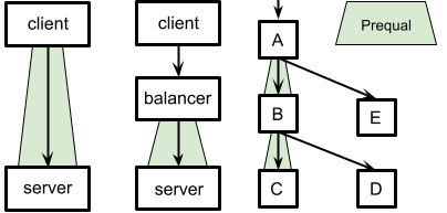
Figure 1: Queries flow down the tree, responses flow up. A separate balancing job is optional on each link. Load balancing policies may vary by link: A $\rightarrow$ B uses Prequal, while B $\rightarrow$ D does not.

Figure 2: Zooming in on any single link from Fig. 1: server replicas respond to queries from client replicas while their machines run antagonist processes. Aggregate utilization (dashed line) may exceed allocation (dotted line) during spikes in demand.

Large-scale services like YouTube are typically composed of many distributed jobs issuing queries among themselves via RPC. Fig. 1 depicts a vastly simplified version with only five jobs, queries flowing down a tree (with the arrows), and responses flowing back up (against the arrows). In any one of these interactions, the job sending the query is called the client job, while the job returning the response is the server job. For instance, on edge A $\rightarrow$ B, A is the client and B is the server, while B is the client on edges B $\rightarrow$ C and B $\rightarrow$ D. To ensure scalability and redundancy, each job is distributed across a large number of machines, called replicas (Fig. 2). To avoid overloading any server replica, a load balancing policy must be used between each pair of communicating jobs, to determine which server replica should receive each query. Some policies require proxying the queries through a separate load balancing job whose only function is to decide where to forward each query, while others can operate directly between client replicas and server replicas (Fig. 1). Prequal is well-suited to both modes of operation, and in fact we use it both ways in different systems at Google.

Each job runs within a single data center, although different jobs might run in different data centers. Each replica runs inside its own virtual machine (VM), which has access to a guaranteed portion of the CPU cycles on its host machine; this amount is called its (CPU) allocation. The fraction of its allocation that a replica uses over any given time period is its (CPU) utilization, which could be more or less than 100%, since the allocation is just a guaranteed minimum. The server job’s aggregate (job) utilization is the fraction of its overall CPU allocation that it uses, across all replicas. In the usual case, each replica has the same allocation, so aggregate job utilization equals average replica utilization.

A server replica typically shares its machine with many other VMs, which we call antagonists. The machine (CPU) utilization accounts for both our server replica and all antagonists, and is distinct from both replica and job utilizations. In order to ensure consistent performance for all users of this multi-tenant system, isolation mechanisms attempt to prevent the behavior of one VM on a machine from adversely affecting the behavior of another. The philosophy here is: "If your usage stays within your allocation, you will be fine." However, if a VM overflows its CPU allocation, it may suffer when the isolation system kicks in.

Given this isolation regime and design philosophy, it seems self-evident that trying to balance CPU utilization across replicas within one job is the best approach. Indeed, the WRR policy works well at Google. It uses smoothed historical statistics on each replica’s goodput, CPU utilization, and error rate to periodically compute individual per-replica weights. Clients then route queries to replicas in proportion to these weights. In the absence of errors, each replica weight $w_{i}$ is calculated as $q_{i}/u_{i}$, where $q_{i}$ and $u_{i}$ represent the recent query-per-second (QPS) rate and CPU utilization of replica $i$. Historically, WRR originated in networking [11] but has also been adapted for replica selection as we just described [4, 9].

We now describe a scenario where this approach backfires, even if we could balance CPU load perfectly. Suppose that our server job has 100 replicas running on identical machines, each replica allocated 40% of the CPU on its machine. Moreover, suppose that antagonist load is soaking up the full remaining 60% on machines 1 and 2, whereas the other 98 machines have ample spare capacity, safely above 4%. Finally, suppose that our job experiences a temporary spike in demand that would raise its aggregate utilization to 1.1x its allocation, i.e., 44% of each machine, on average. A load balancer that attempts to equalize CPU utilization across replicas will aim to peg each replica at this average. All 100 replicas will exceed their CPU allocation, but the last 98 will be okay because the system will let them momentarily spill outside their allocation to soak up the unused CPU cycles. On the heavily contended machines 1 and 2, CPU isolation mechanisms will typically kick in and hobble those replicas, sometimes in ways that affect all queries served by them. Thus, although the problematic load is only the extra 10% on only 2% of our replicas (i.e., ~0.18% of our 1.1x load), it could degrade performance on a full 2% of our queries. Tail latency at p99 is likely to spike. Fig. 6 in Section 5.1 exhibits this behavior on a testbed.

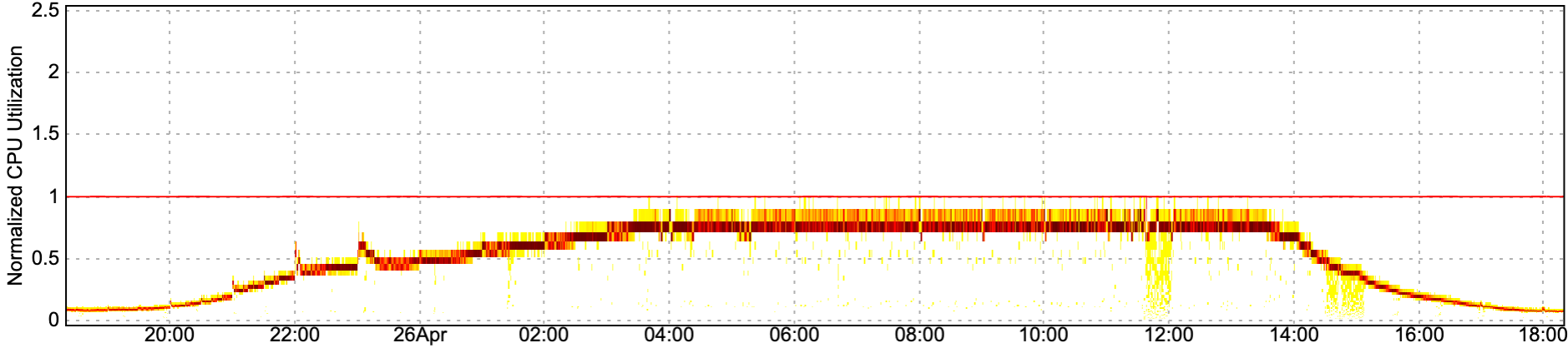
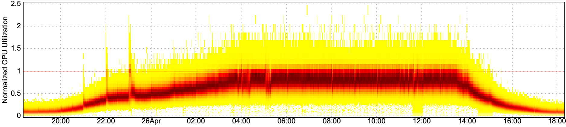
Figure 3: Normalized CPU usage heatmap with 1-minute samples (top) and 1-second samples (bottom) for the YouTube homepage service running across hundreds of machines in a single datacenter. Darker colors represent denser regions. The usage limit, represented by 1.0 (red line) is satisfied in all of the 1m intervals but on 1s intervals it is frequently violated at peak load — sometimes by more than a factor of two!

In this overload case, equalizing replica utilizations was exactly the wrong load-balancing policy because the available machines differed greatly in their capacity to absorb additional load. Furthermore, since the difference in available capacity is due to antagonist processes, it cannot be predicted by our job in advance but can potentially be detected at runtime.

Equalizing replica utilizations can be a great idea if all replicas always stay within their allocation, as this maximizes the amount of traffic we can serve, subject to the allocation. Unfortunately, Fig. 3 shows it is easy to trick ourselves. Plotting CPU utilization over 1m time intervals leads us to believe that the replicas are all respecting their allocations, but using 1s intervals reveals greater underlying variability in the signal, with frequent bursts up to nearly twice the limit! In other words, overload is not really a special case; at sufficiently small timescales, there is nearly always some replica in overload, even if our aggregate load fits within our job allocation. The only questions are whether this replica is unlucky enough to be on a highly contended machine, and whether the spike lasts long enough for isolation mechanisms to kick in.

Thus, avoiding high tail latency requires some mechanism to alert clients quickly about highly-loaded replicas in real-time. The mechanism should use load signals that are as current as possible, and are highly predictive of high latency when serving future requests. CPU utilization fails to meet these criteria, partly because it is a trailing signal. It must be averaged over a time window to be meaningful, which automatically imposes a lower bound on its staleness. This signal also overlooks other factors that contribute to latency, like contention for locks, memory bandwidth, or other shared resources that are sometimes tough to measure or isolate.

Prequal instead uses two load signals: RIF and latency. RIF is an instantaneous signal (i.e., its precise value is available at the time of a probe), and the latency estimates used by Prequal are near-instantaneous as well (Section 4). Here are our main design goals.

1. Minimize probing overheads. The number of probes per query should be a small $O(1)$ and the latency estimation algorithm (running on server replicas) must be lightweight, taking $O(1)$ or $\tilde{O}(1)$ update time per query.

2. Probing should not add significant latency to the query’s critical path. Prequal accomplishes this via asynchronous probing: the current query is assigned using probe responses initiated by previous queries.

3. Minimize tail latency. Prequal removes the worst probes (those with the highest RIF and/or estimated latency) before they can be used for replica selection, in a process inspired by the theory of balanced allocations with memory [14, 16].

4. Limit RAM footprint of query processing on server replicas. Prequal avoids assigning queries to replicas that have an anomalously large RIF, even if their estimated latency is low. The RIF signal does double duty, since it is also a strong leading indicator of future load.

Recall that Prequal can be used either with or without a dedicated load balancing layer (Fig. 1). Advantages of the dedicated layer include (1) keeping probes local when clients query server jobs in a distant data center, (2) the balancer often has fewer replicas than the client does, so each one sees a larger fraction of the query stream, hence its probes are fresher (as measured by number of queries landing on a server replica since the most recent probe), (3) software upgrades to the balancer need not touch the clients. Disadvantages include (1) further RPC overhead (latency, CPU, network), (2) it is an extra job to manage, and (3) one still needs to balance the load arriving at the balancers, although that is usually easier because the balancer’s work is fairly uniform, and it is usually cheaper to overprovision the balancer than the server.

3 Evaluation of deployment in YouTube

A couple of years ago, we identified load imbalance as the cause of persistent SLO violations in YouTube, prompting us to switch some key services to Prequal. These included YouTube’s Homepage service, which is responsible for user-tailored recommendations. With Prequal we saw dramatic improvements across all metrics, including reductions of 2x in tail latency, 5-10x in tail RIF, 10-20% in tail memory usage, 2x in tail CPU utilization, and a near-elimination of errors due to load imbalance. In addition to meeting SLOs, this also allowed us to significantly raise the utilization targets that govern how much traffic we are willing to send to each datacenter, thereby saving significant resources. Based on this success, we rolled out Prequal to many other major services that comprise YouTube, and subsequently to a wide variety of other services at Google, as detailed in Section 1.

The YouTube service is composed of many subsidiary jobs — answering search queries, providing recommendations, and serving ads, to name a few. Queries from some of these jobs trigger a cascade of subsidiary queries, as illustrated in Fig. 1. Since these jobs are so diverse, their query processing requirements (CPU, RAM, latency, etc.) vary widely as well. In this section we show the results of switching from WRR to Prequal using a small subset of live, user-facing traffic for the Homepage job itself, with the load balancing policies in other parts of the system held constant. Historically, the Homepage was the first server job where we deployed Prequal, while most other jobs still used WRR. At the time of this experiment, most but not all of these were using Prequal. In both cases, the impact of the switchover was similar. We state Prequal’s impact here, but defer the details of its design to Section 4. We then explore this design space via experiments on a testbed (not YouTube) in Section 5.

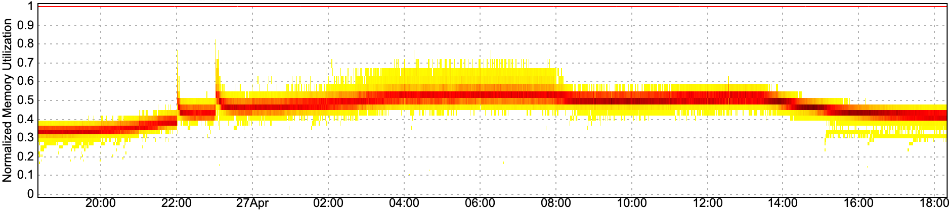
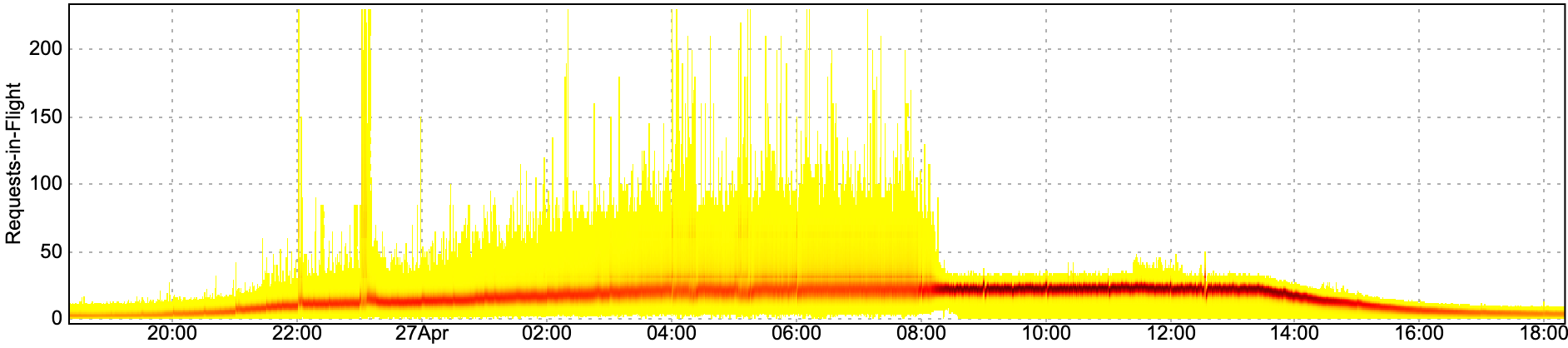
Figure 4: Heatmaps of normalized cpu usage, normalized memory usage, and the number of requests in flight on each YouTube Homepage server replica, first using WRR to balance load before transitioning to Prequal shortly after 08:00.

The first result to notice is that explicitly balancing on RIF really works, bringing down the tail from ~225 to ~50 (Fig. 4). Since Homepage query processing carries a large amount of per-query state, this reduces our tail RAM usage by 10-20%, allowing us to reduce our RAM footprint accordingly. As shown in Fig. 3, WRR was very effective at maintaining a tight CPU load distribution at the 1m time scale, but much poorer when measuring tail CPU utilization at 1s resolution. Prequal fixes that, dropping the tail by ~2x. As a consequence, Prequal decreased occasional server replica error spikes of 0.01-0.1% down to nearly zero and reduced latency by 10-20% at the median and 40-50% at the tail (Fig. 5).

Fig. 5 normalizes each latency quantile (p50, p99, p99.9) separately, based on a typical value for that quantile at the daily traffic trough. This reveals that Prequal does such a good job of pulling in the tail latency at peak load that the p99 and p99.9 actually suffers less at peak (in a multiplicative sense) than p50 does. This is the opposite of the behavior one would normally expect, and that we indeed see for WRR.

For these experiments, we configured Prequal to send 5 probes per query, which means that the total number of RPCs is multiplied by 6. Moreover, as an early adopter of Prequal, this service still uses the synchronous probing mode (Section 4), which adds latency to the critical path. While we intend to migrate to asynchronous probing, our experience with YouTube shows that the improvements we get by pulling in the tails more than compensates for these overheads. This is particularly true for services with relatively heavyweight requests, e.g., $O(10-100)$ milliseconds of processing time per query. We set a 3ms timeout for our probes, but most return far quicker than that. The probing delay and the extra CPU spent on processing the probes are both in the noise compared to the savings.

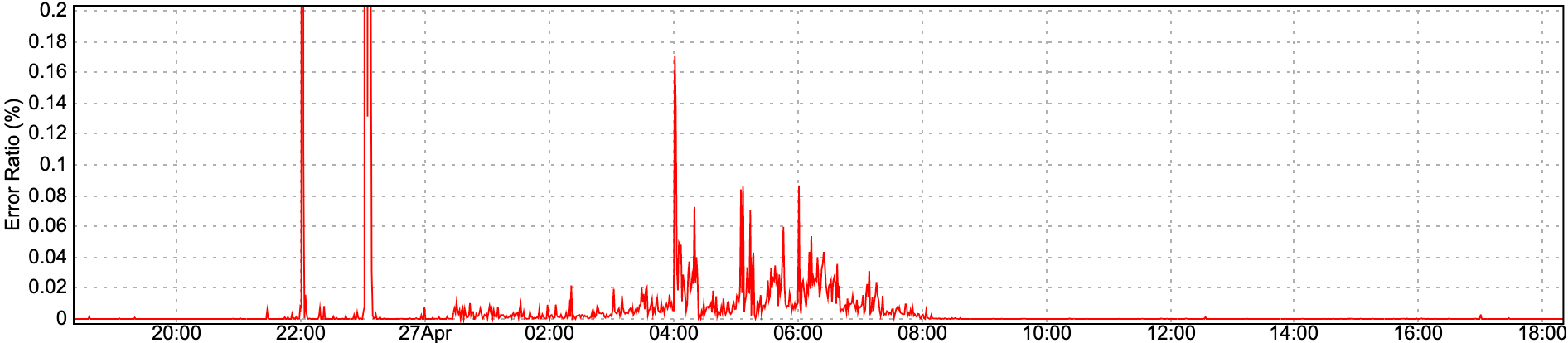
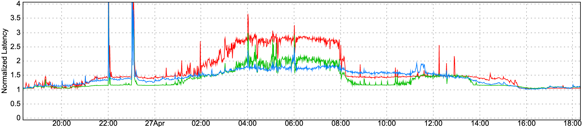
Figure 5: Normalized YouTube Homepage server request error rate and latency p99.9 (red), p99 (green), and p50 (blue). Failures were due to timeouts or load shedding stemming from imbalance. Cutting over from WRR to Prequal shortly after 08:00 eliminated most errors and reduced tail latency by 40-50% and median latency by 5-10%. Each latency quantile is normalized separately to a typical value at daily trough for that quantile, which is why it is possible for the p50 line to lie above the other two after the cutover. The spikes near 22:00 and 23:00 are unrelated to the experiment.

4 System design

When load-balancing a torrent of queries, every millisecond matters. Prequal is designed so that clients can select a replica based on up-to-date information (ideally no more than a few milliseconds old) while keeping the process of sending and receiving probes out of the critical serving path. Hence, the most consequential design decisions center around how to maintain a pool of high-quality probes and how to assign queries to replicas based on the information in the pool. The following are some key questions.

1. How often should a client probe replicas, and which ones should it probe?

2. What information should replicas report in probe responses, and how should they compute it?

3. When selecting a replica to handle a query, how should a client make use of the information in its probe pool?

4. How should a client manage its pool of probe responses? In particular, when should elements be removed?

Probing rate

Clients issue a specified number of probes, $r_{\text{probe}}$, triggered by each query. In addition, they can be configured to issue probes after a specified maximum idle time has been exceeded, to ensure the availability of recent probe responses in the pool even when no queries have arrived in the recent past. The probing rate (per unit time) is therefore the product of the query arrival rate with $r_{\text{probe}}$ (or the minimum probing rate, whichever is greater). We link the probing rate to the query rate because that is the rate at which the client must make decisions. It is also strongly tied to how rapidly the load statistics on the replicas (particularly RIF) change over time, although that also depends on the ratio of client replicas to server replicas. Probing at a rate that greatly exceeds the query arrival rate would thus yield many redundant probes, whereas probing at too low a rate runs the risk that probe results will be “stale” (only weakly correlated with the replica’s current state) by the time they are used.

Probe destinations are sampled uniformly at random without replacement from the set of available replicas. This design choice is motivated by the theory literature on balanced allocations, which advocates sampling a uniformly random set of probe targets. It also helps to avoid the thundering herd phenomenon, when a replica with low estimated latency is inundated with queries from many clients simultaneously seeing it as the best choice, leading to queueing and high latency [15]. This is unlikely to happen in Prequal, where each client’s probe pool represents only a small random subset of replicas, and conversely, each replica belongs to the probe pools of only a small (in expectation) random subset of clients.

We allow $r_{\text{probe}}$ to be fractional , even less than one. Probing consumes a small but nonzero amount of server CPU and network bandwidth, so it is desirable to lower the probing rate to the extent that doing so has only negligible impact on tail latency. Our experiments in Section 5.3 reveal that $r_{\text{probe}}>1$ is quite safe from the standpoint of tail latency.

Load signals

Prequal includes a server-side module for tracking RIF and latency statistics and responding to probes, as follows. We say that the query arrives at the server when the application logic receives the RPC from Stubby, and finishes when the application logic hands the response RPC back to Stubby. We define the latency of the query to be the length of this interval, during which the query contributes to this server’s RIF count. If there is any application-level queueing, then the latency includes the sojourn time in the queue. However, it is more common for the application to eschew queueing and rely on thread or fiber scheduling instead. We do not attempt to capture the network latency, because all server replicas reside in the same datacenter.

When responding to a probe, the RIF comes from simply checking a counter. The latency estimate is more subtle. When a query finishes, we record its latency, tagged by the value of the RIF counter when it arrived. When a probe prompts us to estimate latency, we consult a set of recent latency values at (or near) the current RIF, and report the median. The per-query overhead of maintaining these data structures is small. At moderate-to-high query arrival rates, the samples are plentiful enough that we base the latency estimates entirely on queries that finished in the last O(1-10) milliseconds.

The probe pool

Prequal clients maintain a pool of probe responses to be used in replica selection. Each pool element indicates the replica that responded, the response receipt time, and the load signals discussed above. The pool is capped at a maximum size: we have found that a pool size of 16 suffices to achieve the benefits of Prequal, and the gains from increasing beyond 16 are modest. New probe responses are added to the pool upon receipt, evicting a probe if necessary to respect the maximum pool size.

Replica selection

Prequal could access many load signals, and we have chosen to focus on RIF and latency. The latency signal is obvious: since we want to minimize latency, why not route queries to the replicas exhibiting minimum latency? The RIF part is important because when the replica must store significant per-query state (as in YouTube), its RAM allocation must be a constant offset plus a term that is linear in its max anticipated RIF. In addition, RIF is an instantaneous signal that is a leading indicator of future load, since it represents the queries processing right now. The latency signal is based on observed latencies of queries that have completed recently. Both signals are more up-to-date than CPU utilization, which must be averaged over a long time period to be meaningful.

From the RAM perspective, RIF matters only if our choice of replica raises the max RIF. In principle, we would prefer to balance on latency at all other times, although we must temper this impulse because of the leading versus trailing indicator consideration described above.

To minimize both latency and RIF, Prequal selects replicas using a hot-cold lexicographic (HCL) rule that labels probes in the pool as either hot or cold based on their RIF value. Prequal clients maintain an estimate of the distribution of RIF across replicas, based on recent probe responses. They classify pool elements as hot if their RIF exceeds a specified quantile ($Q_{\text{RIF}}$) of the estimated distribution, otherwise cold. In replica selection, if all probes in the pool are hot, then the one with lowest RIF is chosen; otherwise, the cold probe with the lowest latency is chosen. Our experiments (Section 5.2) suggest that $Q_{\text{RIF}}\in[0.6,0.9]$ is a good choice, although even 0 is effective (i.e., RIF-only control).

An exception arises if the pool is empty. Then, Prequal simply falls back to selecting a uniformly random replica. In fact, our experience suggests it is useful to invoke this fallback whenever the pool occupancy drops below 2.

One popular approach to combining two signals is to use a linear combination of them with a scaling constant to put them into the same units. In our experiments, HCL outperforms RIF-only (Section 5.3), which outperforms every non-trivial linear combination of RIF and latency (Section 5.2 and Appendix A). The HCL approach also nicely captures our hierarchy of concerns: containing latency is nice, but replicas obeying their RAM allocations is often a hard constraint.

Probe reuse and removal

Prequal manages the probe pool to avoid three conditions: staleness, when the load signals are too old to be accurate; depletion, when the pool becomes empty; and degradation, when the loads represented in the pool exhibit a selection bias towards replicas with higher load. These are intertwined and the discussion will necessarily be somewhat circular, so we start with the simplest.

Depletion: Prequal employs several probe removal processes (detailed below) to control staleness and degradation, including removing probes when they are used. In order to stave off pool depletion without increasing the probing rate, we can extend the life of each probe by reusing it up to $b_{\text{reuse}}$ times. This reuse limit is set according to the formula

$$b_{\text{reuse}}=\max\left\{1,\tfrac{1+\delta}{(1-m/n)\cdot r_{\text{probe}}-r_{\text{remove}}}\right\},$$ (1)

where $\delta>0$ is a configuration parameter that governs the net rate at which probes accumulate in the pool, $m$ is the maximum pool size, $n$ is the number of replicas, $r_{\text{probe}}$ is the probing rate discussed above, and $r_{\text{remove}}$ is the rate of probe removal discussed below. We always set $b_{\text{reuse}}\geq 1$, and when it is fractional, we randomly round it to its floor or ceiling so as to preserve the expectation.

Staleness occurs for two reasons: aging and overuse. As a probe ages, its load data becomes less accurate because the replica receives new queries and finishes ones it already had. Overuse is a special case of aging that we can partially mitigate; namely, when the client itself sends a query to that replica, it can compensate by incrementing the RIF value on that probe. Ideally, we would also increase its latency estimate, but currently we do not. Part of Prequal’s solution for general staleness is to set a time limit on probes and remove them from the pool when their age exceeds this limit. In addition, whenever a new probe arrives that would increase the pool beyond its size limit, we drop the oldest probe.

Degradation is the subtlest of these phenomena. If the probes corresponding to lightly-loaded replicas are continually being selected and removed from the pool, then the probes that remain after many rounds of replica selection correspond to highly-loaded replicas. To avoid this, Prequal periodically removes the worst probe from the pool. This is analogous to — but much more permissive than — the use of only the least-loaded of $d$ randomly selected bins in the standard power-of-$d$-choices model. It turns out that broadening the bin-selection policy from “use only the best of $d$ random probes” to “avoid using the worst of $d$ random probes” qualitatively preserves the theoretical guarantees for the power-of-$d$-choices model [21]. When removing the worst probe, Prequal alternates between two rules: removing the oldest probe (i.e., worst age) and removing the probe deemed worst according to the same ranking used for replica selection (but in reverse): if at least one probe in the pool is hot, the hot probe with highest RIF is removed; otherwise, the cold probe with highest latency is removed.

We define a $r_{\text{remove}}$ parameter, and delete that many probes from the pool with each query. As with the probing rate, this number may be fractional, in which case the actual number of probes removed is always either the floor or the ceiling, deterministically rounded to achieve the configured rate of probe removal on average. By alternating our removals between oldest and most loaded, we achieve a unified approach to avoid both staleness and degradation (on top of the probe timeouts).

To summarize, Prequal removes probes from the pool for four reasons. It evicts the oldest probe in the pool when necessary to avoid exceeding the maximum pool size. Probes are removed once they reach their reuse budget or when their age exceeds a timeout threshold. Additionally, they are removed at a configurable rate per query, alternating between worst and oldest.

Synchronous mode

So far, we described Prequal with asynchronous probing (i.e., async mode), which maintains a probe pool to take probing off the critical serving path. The asynchrony is helpful in many use cases, such as when the probe latency is non-negligible or the CPU overhead of probing is high compared to the queries. However, we have also implemented a sync mode of Prequal in which there is no probe pool. Instead, when a query arrives, the client issues some $d$ probes (at least 2, typically 3-5 ) to random replicas , waits to receive a sufficient number of responses (typically $d-1$ ) and then chooses among those using the same replica selection rule described above. We describe the sync mode here because it has been used in YouTube services as reported in Section 3, but all of the experiments reported in Section 5 use async Prequal because that mode is better for most uses.

One significant use case that requires sync mode is when replicas hold state that influences the cost of query execution, e.g., a replica may cache certain data in memory to prevent reading from a slower storage layer. Sync probing allows us to include relevant information from the query in the probe. If the replica then determines that it can execute that query more efficiently because of data it already has in the cache, then it can manipulate its reported load so as to attract the query, e.g., by scaling down its reported load by 10x. We have used sync Prequal in this way for part of YouTube.

Error aversion to avoid sinkholing

Suppose a certain replica has a problem (such as misconfiguration) that causes it to process queries very quickly by immediately returning errors for a non-trivial fraction of its queries. Then its latency on the remaining successful queries, RIF, CPU utilization, and other metrics will make it appear less loaded than it normally would, given the amount of traffic sent its way. If the load balancer is not smart about this, this replica can attract more and more traffic, in a phenomenon known as sinkholing. Prequal includes some heuristics to avoid sinkholing, but since they are not central to our contribution, we have chosen to simplify our exposition by omitting details.

5 Testbed evaluation

In Section 3 we reported on our experience deploying Prequal in YouTube. The comparison between Prequal and WRR in that section constitutes one type of evaluation, under conditions that arguably represent the ground-truth definition of a realistic workload. However, evaluating the deployed version of Prequal in production does not shed light on how individual aspects of its design affect its performance. In this section we report on a set of tests performed on a testbed environment that allows for more controlled experiments with Prequal and baselines, while preserving key features of the production environment for which Prequal was designed: variable query costs and unpredictable time-varying antagonist load.

We first describe our testbed and the baseline system parameters. Within each experiment, we explain which parameters we changed from the baseline.

Our testbed consists of one client job and one server job, each comprising multiple replicas running on distinct but identical physical machines colocated in the same datacenter. The queries represent a very simple CPU-intensive workload: they simply iterate an expensive hash function. In order to simulate variability in query costs, we vary the number of iterations, drawing it from a normal distribution whose standard deviation equals its mean (then truncated at zero). The jobs are running within a standard Google datacenter, on commodity multicore machines, using Google’s standard isolation mechanisms, and the antagonist traffic is just whatever we happen to encounter in the wild.

All experiments use 100 client replicas and 100 server replicas, and each of the server replicas is allocated 10% of the machine’s CPU. In addition, probe pool size = 16, probes age out of the pool after one second, and the net probe-pool drift rate in Equation 1 is $\delta=1$. Unless otherwise specified, we set $Q_{\text{RIF}}$ = $2^{-0.25}\approx 0.84$ and $r_{\text{remove}}$ = 1. We use 3 probes per query as our baseline probe rate to stay safely away from probe rates low enough to impact performance. We target different aggregate utilizations in each experiment as necessary to induce the behaviors we wish to illustrate. Wherever we plot CPU utilization, it is scaled as a percentage of the allocation.

Some of the plots in these experiments show quantiles of RIF values. Since this data is all integer, the quantiles should be integer as well. However, when our monitoring system builds histograms, all instances of an integer $k$ are uniformly smeared across the interval $[k-\frac{1}{2},k+\frac{1}{2})$. For this reason, the plots of our RIF quantiles contain fractional values.

5.1 Robustness to variable antagonist load

Figure 6: Load ramp experiment. Gray background denotes WRR policy, white denotes Prequal. Note that tail latency is plotted on a log scale.

In this experiment, we start with the aggregate CPU load at about 75% of our allocation, and ramp it up in 8 multiplicative steps of 10/9, yielding 0.75x, 0.83x, 0.93x, 1.03x, 1.14x, 1.27x, 1.41x, 1.57x, and 1.74x our allocation. We increased the load by increasing the aggregate query rate from about 5.6k queries per second (henceforth, qps) to around 13k qps, while holding the mean work per query constant. Within each load level, we use WRR for the first half of the period, then Prequal for the second half.

The top plot in Fig. 6 shows the effect on median and tail latency, on a log scale, measured in microseconds. We employ a 5s timeout for each query, so the graph tops out at 5s. In the first three steps (below allocation) the latency distribution stays steady for both WRR and Prequal at roughly 80ms (p50), 182ms (p90), 265ms (p99), and 325ms (p99.9). Then, as soon as we first exceed our CPU allocation (by 1.03x) in step 4, the behaviors of WRR and Prequal rapidly diverge.

For WRR, the p99.9 latency maxes out at the 5s limit, while p99 jumps about 26% to 335ms, slightly above the previous p99.9. By step 6 (1.27x allocation), p99 has maxed out, and p90 is starting to show a visible bump to ~203ms (+11%). By step 8 (1.57x allocation), p90 has maxed out, and even p50 has risen to ~111ms (+39%). By step 9, even p50 has risen to ~150ms (+88%).

In contrast, Prequal suffers almost no visible change at p99.9 in load steps 4 and 5, and by step 6, p99.9 rises only to ~350ms (+8%). It does begin to rise appreciably at load step 7 (1.41x allocation), but even at step 9 it is still contained around 700ms, far from the 5s timeout. Meanwhile p99 latency does not visibly degrade until load step 7, p90 does so around step 8, and p50 does so around step 9.

The second plot shows error rates, which are zero for both WRR and Prequal up through step 3. Note that this is the absolute number of errors per second, not a percentage. WRR starts showing a very small error rate (5 to 20 errors/s) at load step 4. By load step 5, the error rate rises visibly, increasing much faster than the incoming qps. By step 9, more than a quarter of all queries are returning errors. Essentially all of these are "deadline exceeded" errors, from queries that hit their 5s deadline. In contrast, Prequal returns zero errors at all load levels in this experiment.

The bottom plot shows a heatmap of the CPU utilization distributions for WRR and Prequal. Here, one can see that WRR is doing a superb job at accomplishing what it was designed to do: balance CPU load. In contrast, the CPU distribution for Prequal is substantially looser. So why are the latency and error metrics for WRR so bad? It is precisely the explanation that we offered as motivation in Section 2. Digging further into the server-level data for WRR (not pictured), we see a strong correlation between the server replicas with high antagonist load and ones where our latency suffers. Meanwhile, Prequal shifts load away from those server replicas to avoid the worst of the latency impact.

This collection of results explains the title of our paper. Although it is counterintuitive for most people, in this case the load balancer that achieves near-perfect load balance (WRR) is clearly worse (higher errors and latency). That is because the real goal of a load balancer is not to balance load, it is to direct load where capacity is available.

These results are possible only because many server replicas in our system are not fully allocated with antagonists, and at any given moment, many of these antagonists are not using their full CPU allocations. Prequal allows our job to shift load among replicas so as to fit into these cracks of temporary spare capacity. This has two implications for service provisioning: (1) We can provision much more aggressively, because Prequal can deal with transient load spikes. (2) In theory, this could even enable overcommitment, because it enlarges the relevant resource pool from the level of one machine to a much larger set of machines, enabling more effective statistical multiplexing.

5.2 Replica selection rule

In modern datacenters with thousands of machines, it is common for the machines to span multiple hardware generations and processor architectures. When provisioning a job across multiple machines, we can try to account for these differences by applying a performance multiplier to different machine types, e.g., 1 CPU core of type A is equivalent to 1.2 CPU cores of type B. However, it gets tricky to do this well at scale because the performance skew is often highly dependent on the particular workload, e.g., YouTube may be more suited to one of the hardware generations, while Google Maps is better suited to the other. As a result, when our replicas are assigned to machines with different hardware, their effective throughput becomes heterogeneous, and it is the faster machines that exhibit lower latency when unloaded (by definition). In this case, the way to minimize mean latency is to fill the fast machines until their latency degrades to match the slow machines, and then fill both fast and slow together.

There are various ways that a replica selection rule could be designed to fulfill this goal. We experimented with nine replica selection rules ranging from very simple baselines to sophisticated rules used in popular open-source load balancers (e.g. [26]) and in the research literature (e.g. [23]).

In describing the replica selection rules we evaluated, we distinguish between client-local and server-local quantities. The former are measured at the client (or load balancer) itself, the latter are measured at the server replica and reported back to the client (or load balancer). For example, client-local RIF refers to the number of queries the client has sent to the replica that have not yet yielded responses. Server-local RIF refers to the total number of queries the replica has received (from all clients) that it has not yet finished processing. In the literature on load balancing of HTTP traffic there is also a distinction between individual requests and connections; the latter may be long-lived, comprising multiple requests. Since the queries in our work represent short-lived connections, we ignore this distinction in our experiment, treating connections and requests as synonymous.

We evaluated the following replica selection rules.

• Random selects a uniformly random replica.

• Round Robin (RR) cycles through the replicas, keeping track of the most recently chosen one and always selecting the next available replica in cyclic order.

• Weighted Round Robin (WRR) is as described in Section 2.

• Least Loaded (LL) represents the LeastLoaded policy implemented in the NGINX and Envoy reverse proxies [19, 6]. It chooses the available replica with the least client-local RIF, breaking ties in favor of one nearest to the most-recently-chosen replica in cyclic order.

• Least Loaded with Power of Two Choices (LL-Po2C) samples two available replicas uniformly at random and selects the one with the least client-local RIF. This modification of LL is also implemented in NGINX and Envoy.

• YARP-Po2C is a replica selection rule from Microsoft’s YARP reverse proxy library [26] based on power-of-two-choices. All replicas are periodically polled to report their (server-local) RIF. Replica selection is performed by randomly sampling two replicas and selecting the one with lower reported RIF. In our experiments we set the polling interval to 500ms, a 30x faster rate of polling than in the standard YARP-Po2C implementation. We chose the 500ms interval to approximately equalize the total number of RIF reports each client receives, per second, with the number of probe responses received per second by Prequal clients in our experiment.

• Linear, C3, and Prequal all use the asynchronous probing method described in Section 4, but they differ in the scoring rule used to select a replica from the pool of probe responses.

• Linear uses a linear combination of RIF and latency. To represent RIF and latency in comparable units, we scale RIF by the median query processing time measured on replicas with one request in flight. A replica’s score is defined to be an equally weighted average of latency and scaled RIF.

• C3 in this paper uses the replica scoring function described in [23] with Prequal’s probing logic. It computes a RIF estimate for each replica as $\hat{q}=1+os\cdot n+\bar{q}$, where $os$ is the client-local RIF, $n$ is the number of clients participating in the job, and $\bar{q}$ is an exponentially weighted moving average of the server-local RIF. It then computes a score for each replica as $\Psi=(R-\mu^{-1})+\hat{q}^{3}\cdot\mu^{-1}$, where $R$ and $\mu^{-1}$ are exponentially weighted moving averages of the client-local and server-local response time, respectively.

• Prequal uses the HCL replica selection rule described in Section 4, with the RIF limit quantile set to $Q_{\text{RIF}}=0.75$.

Figure 7: Comparison of replica selection rules. Dark portions of bars represent 90th percentile, light portions are 99th percentile. Bars representing latencies exceeding 1.25sec are truncated. Timeouts are represented by ’TO’.

The results of our experiment are depicted in Fig. 7. We tested the replica selection rules at two different levels of aggregate CPU load — 70% and 90% of our allocation — and reported two quantiles of tail latency, the 90th percentile (p90) and 99th percentile (p99).

The replica selection rules that performed best at all load levels and latency quantiles were C3 and Prequal. What these rules have in common is that they incorporate server-local quantities, they penalize high (server-local) RIF severely, and they favor low-latency replicas when there are multiple replicas with low RIF. In the case of Prequal this behavior is evident in the way it distinguishes between hot and cold replicas. In the case of C3 it is implicit in the scoring function’s cubic dependence on estimated queue size, $\hat{q}$: when $\hat{q}$ is near zero it contributes negligibly to the score, but it rapidly grows to predominate the score as $\hat{q}$ moves away from zero.

Comparing C3 and Prequal, one sees a small quantitative advantage for Prequal (3-8%) at all load levels and latency quantiles we tested. Another convenient feature of Prequal’s replica selection rule is that it has a tunable parameter, $Q_{\text{RIF}}$, that allows it to span the full range from RIF-only to latency-only control, depending on the needs of the application. Additionally, Prequal uses fewer signals than C3, simplifying the implementation and monitoring.

It is noteworthy that the LL policy, which bases replica selection on client-local rather than server-local RIF, experiences high p99 latency when load is at 70% of allocated capacity. Even when a server has no active connections from a given client, it can be highly loaded with queries from other clients. If this possibility happens more than 1% of the time, that is enough to impact p99 latency. When load is 90% of allocation, we see that even p90 latency suffers heavily under the LL policy. Combining LL with Po2C improves latency at all load levels and quantiles in our experiments, but the LL-Po2C rule still lags far behind Prequal and C3.

YARP-Po2C’s selection rule using server-local RIF fares better at high load than LL-Po2C which uses client-local RIF, as one might expect. However, its decisions are often based on stale information due to the infrequent polling of replicas, and this adversely affects latency.

Interestingly, the replica selection rule based on a 50-50 linear combination of latency and RIF performed much worse than Prequal’s and C3’s scoring rules. This indicates that a linear function of RIF doesn’t penalize high RIF severely enough compared to C3’s cubic function or Prequal’s strict prioritization of cold replicas over hot ones.

Finally, the WRR policy performed quite well when load was at 70% of allocation, but its p99 latency suffers greatly at 90% load. This is consistent with the results reported in Section 5.1, where WRR experiences a very sharp increase in tail latency in response to a modest increase in aggregate CPU load. (WRR experienced this crossover at different load levels in the two experiments, probably because of differing amounts of antagonist load.)

5.3 Tunable parameters

Prequal has a few tunable parameters that influence its behavior and performance. In this section we evaluate the impact of two of those parameters, probe rate and RIF limit threshold. The first influences the freshness of the load signals used for replica selection, while the second influences the selection rule’s propensity for steering queries toward low estimated latency versus avoiding high RIF.

Figure 8: Probing rate experiment. Rates (top) are expressed in probes/query.

Probing Rate

In the YouTube application, the probes are so light compared to the queries themselves that the probing overhead is negligible. Unfortunately, this is not true for all applications. Thus, we seek to identify the minimum probing rate we can tolerate while retaining the benefits of Prequal.

In this experiment, we ramp down the probing rate from 4x to $\frac{1}{2}$x the query rate, in 6 multiplicative steps of $\sqrt{2}$ each, while keeping the probe removal rate steady at 0.25 per query, and $b_{\text{reuse}}$ increases to compensate, guided by (1). In order to magnify the effects, we ran the system very hot, at roughly 1.5x our CPU allocation throughout.

Fig. 8 shows the resulting latency and RIF, as well as the $\theta_{\text{RIF}}$ control parameter. The take-home point is that Prequal is fairly insensitive to the probing rate until we drop below one probe per query, at which point the negative effects become significant. At probing rates of $\frac{1}{\sqrt{2}}$x and $\frac{1}{2}$x, the tail RIF distributions jump visibly, and this change is echoed by both latency quantiles. Anecdotally, we have observed this phenomenon across many similar experiments, always around 1 probe per query.

RIF Quantile

We now present an experiment to explore the RIF vs latency tradeoff expressed by the quantile that distinguishes hot from cold replicas in the HCL rule. To do this, we designate all of the odd-numbered server replicas (1,3,…,99) as fast, and the even-numbered ones (0,2,…,98) as slow. However, we do not actually seek out servers from different hardware generations. Instead, when generating the queries, we artificially inflate the query work by a factor of 2 on the even replicas, thereby causing it to burn 2x the CPU cycles and act as if it were 2x slower. In addition, we vary the $Q_{\text{RIF}}$ parameter over the course of the experiment, starting at 0 (meaning RIF-only control), then ramping it up from $0.9^{10}\approx 0.35$ to 0.9, in steps of $\frac{10}{9}$, then to 0.99, 0.999, and 1 (meaning latency-only control). Thus, there are 14 steps overall. Throughout this experiment, the mean load is held steady at about 75% of the CPU allocation.

Note that there is actually a discontinuity in the behavior of Prequal between the last two steps. At $Q_{\text{RIF}}$ = 0.999, the RIF limit is effectively the maximum RIF, which means that any replica tied for the max is considered hot. In contrast, when $Q_{\text{RIF}}$ = 1, the RIF limit is $\infty$, and every replica is considered cold.

Figure 9: RIF Limit experiment. $Q_{\text{RIF}}$ varies from 0 at left (pure RIF control) to 1 at right (pure latency control).

Fig. 9 shows the results. The RIF limit threshold $Q_{\text{RIF}}$ increases from 0 on the left (pure RIF control) to 1 on the right (pure latency control). The top two plots show the p99, p90, and p50 latencies. As we would expect, all three latency quantiles go down as we shift more towards latency-based control, up through step 12 ($Q_{\text{RIF}}$ = 0.99). Specifically, p99 drops from ~162ms to ~142ms (-12%), p90 drops from 93ms to 75ms (-19%) and p50 drops from ~34.5ms to ~31ms (-10%). At step 13, all three quantiles begin to edge up slightly. When we switch to full latency control in step 14, all quantiles move up sharply, especially p99, which jumps up from ~148ms (step 13) to about 178ms (+20%). Even more dramatic is p99.9 (not shown), which falls from 210ms in step 0 to 198ms in step 12, rises back to 210ms in step 13, and then fluctuates chaotically in the 337ms to 502ms range in step 14 (1.6x to 2.4x, compared to step 13).

It appears that even a tiny bit of RIF control goes a long way. Why is it that pure latency control results in such worse latency than $Q_{\text{RIF}}$ = 0.999? We hinted at our interpretation earlier: RIF is a valuable leading signal of load, so ignoring it entirely is a bad idea.

The bottom plot shows the CPU utilization distribution. Notice the two crossing bands, which correspond to the “slow” (i.e., even) and “fast” (i.e., odd) replicas. The slow (resp. fast) replicas correspond to the band that is decreasing (resp. increasing) to the right. This is exactly as we would expect, as increasing $Q_{\text{RIF}}$ means we balance more often based on latency, which favors the fast replicas. In addition, the CPU distributions are tighter to the left, where RIF control is higher. This is because RIF is quite a good predictor of future CPU utilization.

This experiment justifies the HCL rule, since turning the dial towards more latency-based control does indeed decrease latency, and turning it up even as high as 0.73 (step 9) has next to no impact on RIF. At step 7 ($Q_{\text{RIF}}$ = 0.59), all three RIF quantiles are just as good as with RIF-only control, despite the fact that the vast majority of queries are being routed based on latency. In this experiment, the probe pool has size 16 and is nearly always full. Because of the use-best and remove-worst processes, the probe pool is not uniformly random. But if it were, then the probability of all 16 probes being hot would be roughly $2^{-16}\approx 1.5\times 10^{-5}$, since $\theta_{\text{RIF}}$ and p50 RIF are both 5 during step 7. Otherwise, the query is routed to a cold replica based on latency. This is what allows us to have the best of both worlds, most of the time: simultaneously routing based on latency and avoiding the highest-RIF replicas.

6 Related work

The “power of two choices” paradigm for randomized load balancing was first analyzed in the highly influential work of Broder et al. [2] and Mitzenmacher [18]. These ideas originated in theoretical work, but over the years they found their way into a wide variety of applications in industry, as noted in the prize citation for the 2020 ACM Paris Kanellakis Theory and Practice Award [1]. The original theoretical results on the power of two choices pertained to the case of throwing $n$ balls into $n$ bins, but they were soon generalized to the “heavily loaded” setting, when balls exceed bins [3]. Qualitatively, these results show that load-balancing processes based on randomly sampling multiple choices and selecting the best ones vastly outperform simpler procedures based on sampling a single bin for each ball. Subsequent theoretical research affirmed that this finding is surprisingly robust to varying the modeling assumptions or the specific rule for selecting among the sampled bins; see, for example, the surveys [17, 25]. Of particular relevance to the design of Prequal is the generalization to load-balancing processes with memory [16, 13, 14], the closest analogue in the theory literature to our use of asynchronous probing.

The need for datacenter task scheduling with sub-second latencies has prompted a great deal of research into decentralized load balancers. Several proposed systems in this branch of the load balancing literature leverage the power-of-$d$-choices (PodC) paradigm. One prominent example is Sparrow [20], a scheduler for highly parallel jobs that each consist of a large number of tasks. Sparrow aims to minimize the job response time, i.e. the time when the last constituent task of a job finishes executing. This goal motivates a different set of design choices, combining batch sampling and late binding: a client whose job comprises $m$ tasks places $d\cdot m$ reservations on randomly selected server replicas; the $m$ replicas that become available soonest request to run the $m$ tasks, and the other $(d-1)\cdot m$ reservations are canceled. This achieves a similar effect to probing $d\cdot m$ replicas and selecting the $m$ best probe responses, with reservations playing the role of probes. Our setting differs in that jobs are not batched, which allows us to substitute a simpler and more efficient probing mechanism, avoiding the use of reservations and late binding which would incur undesirable overheads in our environment. Building upon Sparrow’s batch sampling idea, Eagle [5] is a hybrid scheduler that incorporates a distributed probe-based scheduler using batch sampling to handle short-lived tasks, alongside a centralized scheduler that places long tasks on replicas. The hybrid scheduler design makes sense in settings where a wide disparity in job sizes makes head-of-line blocking a potentially serious problem; in our setting the jobs (queries) are short-lived, allowing the fully distributed load-balancing solution offered by Prequal to perform well in the production environment of YouTube and in our testbed.

A centralized PodC-based load-balancer is incorporated into RackSched [27], where it runs on a top-of-rack switch to make microsecond-scale inter-server scheduling decisions enabling rack-scale computing. Client-based probing solutions such as ours are inapplicable in their setting, where the resource cost of probing is comparable to the resource cost of serving requests. Instead of probing, their servers piggyback load signals into normal traffic and the scheduler treats these load signals as implicit probes. Another rack-scale load balancing system using a RIF-based queueing policy is R2P2 [12], whose $\mathsf{JBSQ}(n)$ policy is a variation on the LeastLoaded policy discussed in Section 5.2. Both RackSched and R2P2 rely on all connections passing through a single router or switch; as explained in Section 2, at the scale of a service such as YouTube using a single load balancer is not a viable option.

C3 [23] is another distributed load balancer with the same design goal as Prequal— minimizing tail latency by adaptively selecting replicas in response to real-time load feedback — but a very different methodology using much more state. C3 uses distributed rate control and backpressure, with every client maintaining exponentially weighted moving average estimates of latency and RIF for every server replica, and using a token-bucket based rate limiter for each server replica. Prequal’s design, in which the only state clients maintain is a probe pool of bounded size, is better suited to load balancing at the scale of a system such as YouTube.

Many existing load balancing systems (e.g., NGINX [19], Envoy [7], Finagle [8], YARP [26]) offer some variant of PodC, and most of them offer (client-local) RIF, latency, or some combination as the load balancing signal. As detailed in Section 5.2, the use of signals local to the client or load-balancer adversely affects performance at scale, when many clients or balancers might be sharing the same pool of replicas.

A number of other production systems leverage PodC load balancing. Netflix’s Zuul [22] incorporates decentralized routing of requests from load balancers to backends by randomly considering two candidates and using a combination of local and piggybacked RIF statistics from previous responses to choose the least-loaded server. Unlike Prequal, Zuul eschews active probing and does not incorporate latency information. NGINX’s implementation [19], like Zuul, is probe-less, but its selection criterion is configurable: “least-connections” uses the lowest RIF from a given balancer to each backend and “least-time” uses estimated latency based on prior requests and the number of current connections. Given our experience with Prequal, we believe it is likely that the performance of the load-balancing mechanisms described in [22, 19] could be improved by supplementing the piggybacked data with active probing.

Appendix A Linear combinations of latency and RIF

Figure 10: Evaluating replica selection rules based on linear combination of latency and RIF.

To evaluate the effectiveness of replica selection rules that use a linear combination of latency and RIF, we used our testbed to experiment with a variant of Prequal that uses the some asynchronous probing method detailed in Section 4, modified to select replicas using a linear combination of latency and RIF. In other words, the HCL replica selection rule was replaced with one that chooses among the replicas represented in the probe pool by minimizing the score

$$\text{score}^{\lambda}_{i}=(1-\lambda)\cdot\text{latency}_{i}+\lambda\cdot\alpha\cdot\text{RIF}_{i}$$ (2)

where $\text{latency}_{i},\,\text{RIF}_{i}$, respectively, denote the latency and RIF in the probe response from replica $i$, $\alpha$ is a scale factor applied to RIF to convert it into the same units as latency, and $\lambda\in[0,1]$ is a tunable parameter that adjusts the relative weight given to latency and RIF. Setting $\lambda=0$ corresponds to latency-only control, whereas $\lambda=1$ corresponds to RIF-only control.

To set the scale factor $\alpha$, we used the approximate median query response time for server replicas with one request in flight. This value turned out to be 75 milliseconds. Note that for any $\alpha>0$, the set of scoring rules $\{\text{score}^{\lambda}\mid 0\leq\lambda\leq 1\}$ obtained by varying $\lambda$ over the interval $[0,1]$ is always equal to the set of convex combinations of latency and RIF. In other words our choice of $\alpha=75\text{ms}$ affects the way that this set of scoring rules is parameterized by $\lambda$, but doesn’t affect the set itself.

We evaluated linear combination scoring rules by measuring quantiles of latency and RIF in our testbed at a constant level of aggregate CPU utilization (equal to 94% of our allocation) while varying $\lambda$. Replicas were partitioned into an equal number of fast (odd-numbered) and slow (even-numbered) ones, with a 2x difference in query processing speed, as in the RIF quantile experiment described in Section 5.3. We initially experimented with varying $\lambda$ over the full range $[0,1]$ in increments of 0.1. It was evident from this initial experiment that linear combination rules with $\lambda\leq 0.7$ performed poorly compared to larger values of $\lambda$, which prompted us to examine the range depicted in Fig. 10 at a finer resolution. Of the 13 linear combinations tested in the experiment, all quantiles of latency and RIF improved monotonically as $\lambda$ increased, with $\lambda=1$ (i.e., RIF-only control) dominating all other linear-combination feedback control rules, in most cases by a wide margin.

Recall from Fig. 9 in Section 5.3 that RIF-only control (represented in that figure by RIF limit threshold 1.0, the rightmost configuration) performs strictly worse than Prequal at all quantiles of latency and RIF. Since the results of the experiment reported here show that RIF-only control performs strictly better than any other linear combination of latency and RIF, it follows by transitivity that Prequal strictly dominates all linear combinations of latency and RIF.

References

- [1] 2020 ACM Paris Kanellakis Theory and Practice Award. https://www.acm.org/media-center/2021/may/technical-awards-2020, 2020. Accessed: 2023-05-02.
- [2] Yossi Azar, Andrei Z. Broder, Anna R. Karlin, and Eli Upfal. Balanced allocations. SIAM J. Comput., 29(1):180–200, 1999.
- [3] Petra Berenbrink, Artur Czumaj, Angelika Steger, and Berthold Vöcking. Balanced allocations: The heavily loaded case. SIAM J. Comput., 35(6):1350–1385, jun 2006.
- [4] Alejandro Forero Cuervo. Load balancing in the datacenter. In Jennifer Petoff, Niall Murphy, Betsy Beyer, and Chris Jones, editors, Site Reliability Engineering: How Google Runs Production Systems, chapter 20, pages 231–247. O’Reilly, Sebastopol, 2016.
- [5] Pamela Delgado, Diego Didona, Florin Dinu, and Willy Zwaenepoel. Job-aware scheduling in eagle: Divide and stick to your probes. In Marcos K. Aguilera, Brian Cooper, and Yanlei Diao, editors, Proceedings of the Seventh ACM Symposium on Cloud Computing, Santa Clara, CA, USA, October 5-7, 2016, pages 497–509. ACM, 2016.
- [6] Envoy github repository. https://github.com/envoyproxy/envoy. Accessed: 2023-09-21.
- [7] Envoy homepage. https://www.envoyproxy.io. Accessed: 2023-09-21.
- [8] Deterministic Aperture: A distributed, load balancing algorithm. https://blog.twitter.com/engineering/en_us/topics/infrastructure/2019/daperture-load-balancer, 2019. Accessed: 2023-09-21.
- [9] gRPC Weighted Round Robin load balancing component. https://github.com/grpc/grpc/tree/master/src/core/ext/filters/client_channel/lb_policy/weighted_round_robin. Accessed: 2023-05-03.
- [10] Chris Jones, John Wilkes, Niall Murphy, and Cody Smith. Service level objectives. In Jennifer Petoff, Niall Murphy, Betsy Beyer, and Chris Jones, editors, Site Reliability Engineering: How Google Runs Production Systems, chapter 4, pages 37–48. O’Reilly, Sebastopol, 2016.
- [11] Manolis Katevenis, Stefanos Sidiropoulos, and Costas Courcoubetis. Weighted round-robin cell multiplexing in a general-purpose ATM switch chip. IEEE Journal on Selected Areas in Communications, 9(8):1265–1279, 1991.
- [12] Marios Kogias, George Prekas, Adrien Ghosn, Jonas Fietz, and Edouard Bugnion. R2P2: Making RPCs first-class datacenter citizens. In 2019 USENIX Annual Technical Conference (USENIX ATC 19), pages 863–880, 2019.
- [13] Dimitrios Los, Thomas Sauerwald, and John Sylvester. Balanced allocations: Caching and packing, twinning and thinning. In Proceedings of the 2022 Annual ACM-SIAM Symposium on Discrete Algorithms (SODA), pages 1847–1874, 2022.
- [14] Dimitrios Los, Thomas Sauerwald, and John Sylvester. Balanced allocations with heterogeneous bins: The power of memory. In Proceedings of the 2023 Annual ACM-SIAM Symposium on Discrete Algorithms (SODA), pages 4448–4477, 2023.
- [15] Michael Mitzenmacher. How useful is old information? IEEE Trans. Parallel Distributed Syst., 11(1):6–20, 2000.
- [16] Michael Mitzenmacher, Balaji Prabhakar, and Devavrat Shah. Load balancing with memory. In The 43rd Annual IEEE Symposium on Foundations of Computer Science, 2002. Proceedings., pages 799–808. IEEE, 2002.
- [17] Michael Mitzenmacher, Andréa W. Richa, and Ramesh Sitaraman. The power of two random choices: A survey of techniques and results. In Sanguthevar Rajasekaran, Panos M. Pardalos, and José Rolim, editors, Handbook of Randomized Computing, volume 1, pages 255–312. Springer Science & Business Media, 2001.
- [18] Michael David Mitzenmacher. The Power of Two Choices in Randomized Load Balancing. PhD thesis, UC Berkeley, 1996.
- [19] Nginx and the “Power of Two Choices” load-balancing algorithm. https://www.nginx.com/blog/nginx-power-of-two-choices-load-balancing-algorithm/, 2018. Accessed: 2023-05-04.
- [20] Kay Ousterhout, Patrick Wendell, Matei Zaharia, and Ion Stoica. Sparrow: Distributed, low latency scheduling. In Proceedings of the 24th ACM Symposium on Operating Systems Principles (SOSP), pages 69–84, 2013.
- [21] Gahyun Park. A generalization of multiple choice balls-into-bins. In Proceedings of the 30th Annual ACM SIGACT-SIGOPS Symposium on Principles of Distributed Computing, pages 297–298, 2011.
- [22] Rethinking Netflix’s edge load balancing. https://netflixtechblog.com/netflix-edge-load-balancing-695308b5548c, 2018. Accessed: 2023-05-04.
- [23] Lalith Suresh, Marco Canini, Stefan Schmid, and Anja Feldmann. C3: Cutting tail latency in cloud data stores via adaptive replica selection. In 12th USENIX Symposium on Networked Systems Design and Implementation (NSDI 2015), pages 513–527, 2015.
- [24] Varun Talwar. gRPC: a true internet-scale RPC framework is now 1.0 and ready for production deployments. https://cloud.google.com/blog/products/gcp/grpc-a-true-internet-scale-rpc-framework-is-now-1-and-ready-for-production-deployments, 2016. Accessed: 2023-09-21.
- [25] Udi Wieder. Hashing, load balancing and multiple choice. Foundations and Trends® in Theoretical Computer Science, 12(3–4):275–379, 2017.
- [26] YARP: Yet Another Reverse Proxy. https://microsoft.github.io/reverse-proxy/. Accessed: 2023-09-21.
- [27] Hang Zhu, Kostis Kaffes, Zixu Chen, Zhenming Liu, Christos Kozyrakis, Ion Stoica, and Xin Jin. Racksched: A microsecond-scale scheduler for rack-scale computers. In 14th USENIX Symposium on Operating Systems Design and Implementation, OSDI 2020, pages 1225–1240. USENIX Association, 2020.