Secret extraction attacks against obfuscated IQP circuits

Abstract

Quantum computing devices can now perform sampling tasks which, according to complexity-theoretic and numerical evidence, are beyond the reach of classical computers. This raises the question of how one can efficiently verify that a quantum computer operating in this regime works as intended. In 2008, Shepherd and Bremner proposed a protocol in which a verifier constructs a unitary from the comparatively easy-to-implement family of so-called IQP circuits, and challenges a prover to execute it on a quantum computer. The challenge problem is designed to contain an obfuscated secret, which can be turned into a statistical test that accepts samples from a correct quantum implementation. It was conjectured that extracting the secret from the challenge problem is -hard, so that the ability to pass the test constitutes strong evidence that the prover possesses a quantum device and that it works as claimed. Unfortunately, about a decade later, Kahanamoku-Meyer found an efficient classical secret extraction attack. Bremner, Cheng, and Ji very recently followed up by constructing a wide-ranging generalization of the original protocol. Their IQP Stabilizer Scheme has been explicitly designed to circumvent the known weakness. They also suggested that the original construction can be made secure by adjusting the problem parameters. In this work, we develop a number of secret extraction attacks which are effective against both new approaches in a wide range of problem parameters. The important problem of finding an efficient and reliable verification protocol for sampling-based proofs of quantum supremacy thus remains open.

1 Introduction

A central challenge in the field of quantum advantage is to devise efficient quantum protocols that are both classically intractable and classically verifiable, while minimising the experimental effort required for an implementation. The paradigmatic approach satisfying these first conditions is to solve public-key cryptography schemes using Shor’s algorithm. However, the quantum resources required in the cryptographically secure regime are enormous, using thousands of qubits and millions of gates [see e.g. 1, 2]. Reducing the required resources, interactive proofs of computational quantumness have been proposed, which make use of classically or quantum-secure cryptographic primitives [3, 4, 5]. Again, however, their implementation requires arithmetic operations, putting the advantage regime far beyond the reach of current technology [6].

A different approach to demonstrations of quantum advantage has focused on simple protocols based on sampling from the output of random quantum circuits [7, 8, 9, 10, 11, 12]. These require a significantly smaller amount of qubits and gates, and seem to be classically intractable even in the presence of noise on existing hardware [13, 14, 15, 16]. However, they are not efficiently verifiable (see Ref. [17] for a discussion), and already present-day experiments are outside of the regime in which the samples can be efficiently checked.

The key property which makes random quantum sampling so much more feasible compared to cryptography-based approaches is their apparent lack of structure in the sampled distribution. At the same time, this is also what seems to thwart classical verifiability. Yamakawa and Zhandry [18] have made significant progress by showing that there are also highly unstructured -problems based on random oracles, which can be efficiently solved by a quantum computer and checked by a classical verifier. Conversely, one may wonder whether it is possible to introduce just enough structure into random quantum circuits to make their classical outputs efficiently verifiable while keeping the resource requirements low [19, 20, 21]. An early and influential idea of this type dating back to 2008 is the one of Shepherd and Bremner [19].

Shepherd and Bremner proposed a sampling-based scheme based on so-called IQP (Instantaneous Quantum Polynomial-Time) circuits. In the IQP paradigm, one can only execute gates that are diagonal in the $X$-basis. They designed a family of IQP circuits based on quadratic residue codes (QRC) whose output distribution has high weight on bit strings $\mathbf{x}\in\mathbbm{F}_{2}^{n}$ that are contained in a hyperplane $\mathbf{s}^{T}\mathbf{x}=0\mod 2$. The normal vector $\mathbf{s}\in\mathbbm{F}_{2}^{n}$ may be chosen freely, but its value is not apparent from the circuit description. This way, a verifier can design a circuit that hides a secret $\mathbf{s}$. The verifier then challenges a prover to produce samples such that a significant fraction of them lie in the hyperplane orthogonal to $\mathbf{s}$. At the time, the only known way to efficiently meet the challenge was for the prover to collect the samples by implementing the circuit on a quantum computer. More precisely, Shepherd and Bremner conjectured that it was an -hard problem to recover the secret from $\mathbf{H}$. They challenged the community to generate samples which have high overlap with a secret 244-bit string—corresponding to a 244-qubit experiment.

Unfortunately, in 2019, Kahanamoku-Meyer [22] solved the challenge and recovered the secret string. The paper provided evidence that the attack has only quadratic runtime for the QRC construction.

Recently, Bremner, Cheng, and Ji [23] have made new progress on this important problem. They propose a wide-ranging generalization of the construction—the IQP Stabilizer Scheme—which circumvents Kahanamoku-Meyer’s analysis. They also conjecture that an associated computational problem—the Hidden Structured Code (HSC) Problem—cannot be solved efficiently classically for some parameter choices and pose a challenge for an IQP experiment on 300 qubits, corresponding to a 300-bit secret. Finally, they also extend the QRC-based construction to parameter regimes in which Kahanamoku-Meyer’s ansatz fails.

Here, we show that the scheme is still vulnerable to classical cryptanalysis by devising a number of secret extraction attacks against obfuscated IQP circuits. Our first approach, the Radical Attack instantly recovers the 300-bit secret of the challenge from the circuit description. We analyse the Radical Attack in detail and give conditions under which we expect the ansatz to work. The theory is tested on 100k examples generated by a software package provided as part of [23], and is found to match the empirical data well. We also observe that for the Extended QRC construction, the Radical Attack and the approach of Kahanamoku-Meyer complement each other almost perfectly, in the sense that for every parameter choice, exactly one of the two works with near-certainty.

In the final part of the paper, we sketch a collection of further approaches for recovering secretes hidden in IQP circuits. Concretely, we propose two extensions of Kahanamoku-Meyer’s idea, which we call the Lazy Linearity Attack and the Double Meyer. The Double Meyer Attack is effective against the Extended QRC construction for all parameter choices, and we expect that its runtime is at most quasipolynomial on all instances of the IQP Stabilizer Scheme. Finally, we introduce Hamming’s Razor, which can be used to identify redundant rows and columns of the matrix that were added as part of the obfuscation procedure. For the challenge data set, this allows us to recover the secret in an alternate fashion and we expect it to reduce the load on further attacks in general.

The important problem of finding cryptographic obfuscation schemes for the efficient classical verification of quantum circuit implementations therefore remains open.

We begin by setting up some notation in Section 2, then recall the IQP Stabilizer Scheme in Section 3, describe and analyze the Radical Attack in Section 4, and sketch further exploits in Section 5.

2 Notation and definitions

We mostly follow the notation of Ref. [23]. This means using boldface for matrices $\mathbf{M}$ and column vectors $\mathbf{v}$ (though basis-independent elements of abstract vector spaces are set in lightface). We write $\mathbf{M}_{i}$ for the $i$-th column of a matrix and $\mathbf{v}_{i}$ for the $i$-th coefficient of a column vector. By the support of a set $S\subset\mathbbm{F}_{2}^{m}$, we mean the union of the supports of its elements:

$$\operatorname{supp}V=\{i\in[1,m]\,|\,\exists\,\mathbf{v}\in V,\>\mathbf{v}_{i}\neq 0\}.$$

We use $\mathbf{e}^{i}$ for the standard basis vector $(\mathbf{e}^{i})_{j}=\delta_{ij}$. The all-ones vector is $\mathbf{1}$, and for a set $S$, $\mathbf{1}_{S}$ is the “indicator function on $S$”, i.e. the $i$th coefficient of $\mathbf{1}_{S}$ is $1$ if $i\in S$ and 0 else. The Hamming weight of a vector $\mathbf{v}\in\mathbbm{F}_{2}^{n}$ is $|\mathbf{v}|\coloneqq\sum_{i\in[n]}\mathbf{v}_{i}$.

2.1 Symmetric bilinear forms

Compared to Ref. [23], we use slightly more geometric language. The relevant notions from the theory of symmetric bilinear forms, all standard, are briefly recapitulated here.

Let $V$ be a finite-dimensional vector space over a field $\mathbbm{F}$, endowed with a symmetric bilinear form $\beta(\cdot,\cdot)$. The orthogonal complement of a subset $W\subset V$ is

$$W^{\perp}=\{x\in V\,|\,\beta(x,w)=0\>\forall\,w\in W\}.$$

The radical of $V$ is $V\cap V^{\perp}$, which is the space comprising elements $x\in V$ such that the linear function $\beta(x,\cdot)$ vanishes identically on $V$. The space $V$ is non-degenerate if $\operatorname{rad}V=\{0\}$. In this case, for every subspace $W\subset V$, we have that $\dim W^{\perp}+\dim W=\dim V$. The subspace $W$ is isotropic if $W\subset W^{\perp}$. The above dimension formula implies that isotropic subspaces $W$ of a non-degenerate space $V$ satisfy $\dim W\leq\frac{1}{2}\dim V$.

Let $\{b^{(i)}\}_{i=1}^{k}$ be a basis of $V$. Expanding vectors $x,y\in V$ in the basis,

$$\beta(x,y)=\beta\left(\sum_{i}\mathbf{c}_{i}b^{(i)},\sum_{j}\mathbf{d}_{j}b^{(j)},\right)=\sum_{ij}\mathbf{c}_{i}\mathbf{c}_{j}\,\beta\left(b^{(i)},b^{(j)}\right)=\mathbf{c}^{T}\mathbf{M}\mathbf{d},$$

where $\mathbf{c},\mathbf{d}\in\mathbbm{F}^{k}$ are column vectors containing the expansion coefficients of $x,y$ respectively, and the matrix representation $\mathbf{M}$ of $\beta$ has elements

$$\mathbf{M}_{ij}=\beta\left(b^{(i)},b^{(j)}\right).$$

A vector $x\in V$ lies in the radical if and only if its coefficients $\mathbf{c}$ lie in the kernel of $\mathbf{M}$.

Now assume that $V\subset\mathbbm{F}^{m}$. The standard form on $\mathbbm{F}^{m}$ is

$$\langle\mathbf{x},\mathbf{y}\rangle=\mathbf{x}^{T}\mathbf{y}=\sum_{i=1}^{m}\mathbf{x}_{i}\mathbf{y}_{i}.$$

The standard form is non-degenerate on $\mathbbm{F}^{m}$, but will in general be degenerate on subspaces. Let $\mathbf{H}$ be an $m\times k$ matrix and let $W=\operatorname{range}\mathbf{H}\subset V$ be its column span. The restriction of the standard form to $W$ can then be “pulled back” to $\mathbbm{F}^{k}$ by mapping $\mathbf{c},\mathbf{d}\in\mathbbm{F}^{k}$ to

$$\langle\mathbf{H}\mathbf{c},\mathbf{H}\mathbf{d}\rangle=(\mathbf{H}\mathbf{c})^{T}(\mathbf{H}\mathbf{d})=\mathbf{c}^{T}\big{(}\mathbf{H}^{T}\mathbf{H}\big{)}\mathbf{d}=\mathbf{c}^{T}\mathbf{G}\mathbf{d},$$

where $\mathbf{G}=\mathbf{H}^{T}\mathbf{H}$ is the Gram matrix associated with $\mathbf{H}$. We frequently use the fact that in this context,

$$\mathbf{d}\in\ker\mathbf{G}\qquad\Leftrightarrow\qquad\mathbf{H}\mathbf{d}\in\operatorname{rad}W.$$ (1)

3 The IQP Stabilizer Scheme

3.1 Hiding a secret string in an IQP circuit

The IQP Stabilizer Scheme of Shepherd and Bremner, described here following the presentation in Ref. [23], uses the tableau representation of a collection of $m$ Pauli matrices on $n$ qubits as an $m\times 2n$ binary matrix. Since IQP circuits are diagonal in the $X$ basis, we restrict to $X$-type Pauli matrices which are described by $m\times n$ matrices with elements in $\mathbbm{F}_{2}$. The tableau matrix $\mathbf{H}\in\mathbbm{F}_{2}^{m\times n}$ determines an IQP Hamiltonian $H=\sum_{i\in[m]}(\prod_{j\in[n]}X_{j}^{\mathbf{H}_{ij}})$, with associated IQP circuit $\omega^{H}$ defined in terms of a phase $\omega$. Choosing $\omega=e^{i\pi/4}$ Shepherd and Bremner, observe that the full stabilizer tableau of the state $\omega^{H}\mbox{$|0\rangle$}$ can be expressed in terms of $\mathbf{H}$ and use this fact to find IQP circuits whose output distributions have high weight on a subspace $S_{\mathbf{s}}=\{\mathbf{x}:\langle\mathbf{x},\mathbf{s}\rangle=0\}$ determined by a secret string $\mathbf{s}$.

This is ingeniously achieved as follows. For $\mathbf{s}\in\mathbbm{F}_{2}^{n}$, obtain $\mathbf{H}_{\mathbf{s}}$ from $\mathbf{H}$ by multiplying its $i$-th row with $(\mathbf{H}\mathbf{s})_{i}$. Let $\mathcal{C}_{\mathbf{s}}\coloneqq\operatorname{range}\mathbf{H}_{\mathbf{s}}$. Fix some $g_{\max}\in\mathbbm{N}$. A vector $\mathbf{s}\in\mathbbm{F}_{2}^{n}$ is called a secret of $\mathbf{H}$ if

1. the co-dimension of the radical $g\coloneqq\dim\mathcal{C}_{\mathbf{s}}-\dim\operatorname{rad}\mathcal{C}_{\mathbf{s}}\leq g_{\max}$, and

2. the radical is doubly even, i.e., for all $\mathbf{x}\in\operatorname{rad}\mathcal{C}_{s}$, $|\mathbf{x}|=0\mod 4$.

Given an IQP tableau $\mathbf{H}$ with secret $\mathbf{s}$, Shepherd and Bremner show that

$$\Pr_{\mathbf{x}\leftarrow D_{\mathbf{H}}}[\langle\mathbf{x},\mathbf{s}\rangle=0]=\frac{1}{2}(2^{-g/2}+1),$$ (2)

where $D_{\mathbf{H}}(\mathbf{x})=|\mbox{$\langle x|$}\omega^{H}\mbox{$|0\rangle$}|^{2}$ is the output distribution of $\omega^{H}$. A classical verifier can that efficiently identify samples from the correct distribution by computing their mean overlap with the secret string $\mathbf{s}$.

3.2 Stabilizer construction

We briefly recap the specifics of how Bremner, Cheng, and Ji [23] construct a pair $(\mathbf{H},\mathbf{s})$, comprising a generator matrix $\mathbf{H}$ and corresponding secret $\mathbf{s}$. Pre-obfuscation, the matrix $\mathbf{H}$ is of the following form:

(3)

Essentially, the blocks are chosen uniformly at random, subject to the following constraints:

1. $\mathbf{D}$ is an $m_{1}\times d$-matrix. Its range is a $d$-dimensional doubly-even isotropic subspace of $\mathbbm{F}_{2}^{m_{1}}$. These constraints are equivalent to

   $$|\mathbf{D}_{i}|=0\mod 4\>(i=1,\dots,d),\qquad\mathbf{D}^{T}\mathbf{D}=0,\qquad\operatorname{rank}\mathbf{D}=d.$$ (4)

2. $\mathbf{F}$ is an $m_{1}\times g$-matrix. It generates a $g$-dimensional space that is non-degenerate and orthogonal to $\operatorname{range}\mathbf{D}$ with respect to the standard form on $\mathbbm{F}_{2}^{m_{1}}$. These constraints are equivalent to

   $$\operatorname{rank}\mathbf{F}^{T}\mathbf{F}=g,\qquad\mathbf{D}^{T}\mathbf{F}=0.$$ (5)

3. There exists a secret $\mathbf{s}\in\mathbbm{F}_{2}^{n}$ such that the inner product between $\mathbf{s}$ and the rows of $\mathbf{H}$ is non-zero exactly for the first $m_{1}$ rows:

   $$\mathbf{H}\mathbf{s}=\mathbf{1}_{[1,\dots,m_{1}]}.$$ (6)

4. Finally, $\mathbf{R}_{\mathbf{s}}=(\mathbf{A}\,|\,\mathbf{B}\,|\,\mathbf{C})$ are “redundant rows”, chosen such that $\mathbf{R}_{\mathbf{s}}\mathbf{s}=\mathbf{0}$ and

   $$\operatorname{rank}\mathbf{H}=n.$$ (7)

Further comments:

• Introducing notation not used in [23], we split $\mathbf{R}_{\mathbf{s}}$ into sub-matrices $\mathbf{R}_{\mathbf{s}}=(\mathbf{A}\,|\,\mathbf{B}\,|\,\mathbf{C})$ according to $\mathbbm{F}_{2}^{n}=\mathbbm{F}_{2}^{g}\oplus\mathbbm{F}_{2}^{d}\oplus\mathbbm{F}_{2}^{n-g-d}$.

• It will turn out that the parameter

  $$w:=n-g-m_{2}$$

  plays a central role for the performance the Radical Attack. It may be described as measuring the degree to which the matrix $(\mathbf{B}\,|\,\mathbf{C})$ is “wide” rather than “tall”.

• The range of $\mathbf{H}_{\mathbf{s}}$ is the code space $\mathcal{C}_{\mathbf{s}}$. The range of $\mathbf{D}$ is its radical $\operatorname{rad}\mathcal{C}_{\mathbf{s}}\subset\mathcal{C}_{\mathbf{s}}$. The range of $\mathbf{F}$ is a subspace that is complementary to the radical within the code space.

• The rank constraint (7) implies

  $$\operatorname{rank}\mathbf{C}=n-g-d.$$ (8)

• There are some subtleties connected to the way the redundant rows are generated according to the paper [23] and the various versions of the software implementation provided. See Appendix A for more details.

The parameters $n$ (number of qubits), $m$ (terms in the Hamiltonian), and $g$ (log of the power of the statistical test) are supplied by the user, while $m_{1}$ and $d$ are chosen randomly. The precise way in which $m_{1},d$ are to be generated does not seem to be specified in the paper, so we take guidance from the reference implementation provided at Ref. [24]. Their sample_parameters()-function (found in lib/construction.py) fixes these numbers in a two-step procedure. First, preliminary values of $m_{1}/2$ and $d$ are sampled according to binomial distributions with parameters roughly given as

$$m_{1}/2\sim\operatorname{Bin}\left(N\approx\frac{m-g}{2},p=0.3\right),\qquad d\sim\operatorname{Bin}\left(N=\left\lfloor\frac{m_{1}-g}{2}\right\rfloor,p=0.75\right).$$ (9)

The values are accepted if they satisfy the constraints

$$n-g\leq d\leq w.$$ (10)

We are not aware of a simple description of the distribution conditioned on the values passing the test. Empirically, we find that for the challenge parameters

$$n=300,\quad m=360,\quad g=4,$$ (11)

the following values are attained most frequently:

$$m_{1}=102,\quad d=38\qquad\Rightarrow\qquad m_{2}=258,\quad w=38.$$ (12)

Given $(\mathbf{H},\mathbf{s})$, obfuscation is then performed as $\mathbf{H}\leftarrow\mathbf{P}\mathbf{H}\mathbf{Q}$, $\mathbf{s}\leftarrow\mathbf{Q}^{-1}\mathbf{s}$ using a random invertible matrix $\mathbf{Q}$ and a random (row-)permutation $\mathbf{P}$.

Bremner, Cheng, and Ji pose the following conjecture:

Conjecture 1 (Hidden Structured Code (HSC) Problem [23]).

For certain appropriate choices of $n,m,g$, there exists an efficiently samplable distribution over instances $(\mathbf{H},\mathbf{s})$ from the family $\mathcal{H}_{n,m,g}$, so that no polynomial-time classical algorithm can find the secret $s$ given $n$, $m$ and $\mathbf{H}$ as input, with high probability over the distribution on $\mathcal{H}_{n,m,g}$.

3.3 Extended QRC construction

In the original QRC construction of Shepherd and Bremner [19], $(\mathbf{F}\,|\,\mathbf{D})$ is chosen as a $q\times(q+1)/2$ quadratic residue code with prime $q$ such that $q+1\mod 8=0$. Then, the all-ones vector $\mathbf{1}_{q}$, which is guaranteed to be a codeword of a QRC, is appended as the first column of $(\mathbf{F}\,|\,\mathbf{D})$. Next, rows are added which are uniformly random, except for the first entry which is $0$. This ensures that there is a secret $\mathbf{s}=\mathbf{e}_{1}$. The resulting matrix is then obfuscated as above.

In the Extended QRC construction, additional redundant columns are added, essentially amounting to a nontrivial choice of $\mathbf{C}$, in order to render the algorithm of Kahanamoku-Meyer ineffective. Letting $r=(q+1)/2$, Bremner, Cheng, and Ji propose to add $q$ redundant rows to achieve $m=2q$, and add a redundant $\mathbf{C}$ block to achieve a width $n$ satisfying $r\leq n\leq q+r$.

4 The Radical Attack

Starting point of the attack was the empirical observation that $\mathbf{H}^{T}\mathbf{H}$ for the challenge generator matrix has a much larger kernel ($\dim\ker\mathbf{H}^{T}\mathbf{H}=34$) than would be expected for a random matrix of the same shape (about $1$). This observation gave rise to the Radical Attack, summarized in Algorithm 1.

Algorithm 1 Radical Attack

1:function RadicalAttack($\mathbf{H}$)

2:     $\mathbf{G}\leftarrow\mathbf{H}^{T}\mathbf{H}$

3:     $\mathbf{K}\leftarrow$ a column-generating matrix for $\ker\mathbf{G}$

4:     $S\leftarrow$ the support of the columns in $\mathbf{H}\mathbf{K}$

5:     Solve the $\mathbbm{F}_{2}$-linear system $\mathbf{H}\mathbf{s}=\mathbf{1}_{S}$

6:     return $\mathbf{s}$

7:end function

We have tested this ansatz against instances created by the software package provided by Bremner, Cheng, and Ji. For the parameters $(n,m,g)=(300,360,4)$, used for the challenge data set, the secret is recovered with probability about $99.85\%$. The challenge secret itself can be found using a mildly strengthened version.

We will analyze this behavior theoretically in Sec. 4.1, report on the numerical findings in Sec. 4.2, and, in Sec. 4.3, explain why the challenge Hamiltonian requires a modified approach.

4.1 Performance of the attack

The analysis combines three ingredients:

1. We will show that with high probability, $\mathbf{H}(\ker\mathbf{G})$ is a subspace of the radical $\operatorname{rad}\mathcal{C}_{\mathbf{s}}$. Because $\mathbf{H}$ and thus $\mathbf{G}=\mathbf{H}^{T}\mathbf{H}$ are known, this means that we can computationally efficiently access elements of the radical.

2. We will then show that the intersection of $\mathbf{H}(\ker\mathbf{G})$ with the radical is expected to be relatively large.

These two statements follow as Corollary 3 from a structure-preserving normal form for obfuscated generator matrices of the form (3), described in Lemma 2.

1. In Lemma 4, we argue that one can expect that the non-zero coordinates that show up in this subspace coincide with the obfuscated coordinates $1\ldots m_{1}$.

4.1.1 A normal form for generator matrices

Recall the notion of elementary column operations on a matrix, as used in the context of Gaussian elimination. Over $\mathbbm{F}_{2}$, these are (1) exchanging two columns, and (2) adding one column to another one. Performing a sequence of column operations is equivalent to applying an invertible matrix from the right. We will map the generator matrix $\mathbf{H}$ to a normal form using a restricted set of column operations. These column operations preserve the properties of the blocks of $\mathbf{H}$ described in Section 3.

To introduce the normal form, split $\mathbf{H}$ into blocks as

$$\mathbf{H}=(\mathbf{\hat{A}}\,|\,\mathbf{\hat{B}}\,|\,\mathbf{\hat{C}}),\qquad\hat{\mathbf{A}}:=\begin{pmatrix}\mathbf{F}\\ \mathbf{A}\end{pmatrix},\quad\hat{\mathbf{B}}:=\begin{pmatrix}\mathbf{D}\\ \mathbf{B}\end{pmatrix},\quad\hat{\mathbf{C}}:=\begin{pmatrix}\mathbf{0}\\ \mathbf{C}\end{pmatrix}.$$

We say that an elementary column operation is directed to the left if it

• adds a columns of $\hat{\mathbf{C}}$ to another colum in $(\hat{\mathbf{A}}\,|\,\hat{\mathbf{B}}\,|\,\hat{\mathbf{C}})$,

• adds a column of $\hat{\mathbf{B}}$ to another column in $(\hat{\mathbf{A}}\,|\,\hat{\mathbf{B}})$,

• adds a column of $\hat{\mathbf{A}}$ to another column in $\hat{\mathbf{A}}$, or

• permutes two columns within one block.

The first part of the following lemma lists properties that are preserved under such column operations. The second part describes two essential simplifications to $\mathbf{H}$ which can still be achieved.

Lemma 2 (Normal form).

Assume $\mathbf{H}^{\prime}$ results from $\mathbf{H}$ by a sequence of column operations that are directed to the left. Then:

1. If $\mathbf{H}$ is a block matrix of the form (3) and fulfills the conditions (5) – (7), then the same is true for $\mathbf{H}^{\prime}$.

2. It holds that:

   $$\operatorname{range}(\mathbf{F}^{\prime}\,|\,\mathbf{D}^{\prime}) =\operatorname{range}(\mathbf{F}\,|\,\mathbf{D}),$$

   $$\operatorname{range}\mathbf{D}^{\prime} =\operatorname{range}\mathbf{D},$$

   $$\operatorname{range}(\mathbf{B}^{\prime}\,|\,\mathbf{C}^{\prime}) =\operatorname{range}(\mathbf{B}\,|\,\mathbf{C}).$$

There is a sequence of column operations directed to the left such that:

1. If $\operatorname{range}(\mathbf{B}\,|\,\mathbf{C})=\mathbbm{F}_{2}^{m_{2}}$, then $\mathbf{A}^{\prime}=0$.

2. In any case, $\dim\ker\mathbf{B}^{\prime}\geq w$.

Proof.

Claim 1 and 2 follow directly from the definitions. Least trivial is the statement that Condition (5) is preserved, so we make this one explicit. Consider the case where the $i$-th column of $\hat{\mathbf{B}}$ is added to the $j$-th column of $\hat{\mathbf{A}}$. This will change $\mathbf{F}\mapsto\mathbf{F}^{\prime}=\mathbf{F}+\mathbf{D}_{i}\,(\mathbf{e}^{j})^{T}$. But then, by (4),

$$(\mathbf{F}^{\prime})^{T}\mathbf{F}^{\prime}=\mathbf{F}^{T}\mathbf{F}+\mathbf{e}^{j}\,\mathbf{D}_{i}^{T}\mathbf{F}+\mathbf{F}^{T}\mathbf{D}_{i}\,(\mathbf{e}^{j})^{T}+\mathbf{e}^{j}\,\mathbf{D}_{i}^{T}\mathbf{D}_{i}\,(\mathbf{e}^{j})^{T}=\mathbf{F}^{T}\mathbf{F}.$$

Claim 3 is now immediate: Assuming the range condition, every column of $\mathbf{A}$ can be expressed as a linear combination of columns in $(\mathbf{B}\,|\,\mathbf{C})$. Therefore, $\mathbf{A}$ may be eliminated by column operations directed to the left.

To prove Claim 4, choose a basis $\{\mathbf{b}^{i}\}_{i=1}^{k}$ for $\operatorname{range}\mathbf{B}\cap\operatorname{range}\mathbf{C}$. Using column operations within $\hat{\mathbf{B}}$ and $\hat{\mathbf{C}}$ respectively, we can achieve that the first $k$ columns of $\mathbf{B}$ and of $\mathbf{C}$ are equal to $\mathbf{b}^{1},\ldots,\mathbf{b}^{k}$. The first $k$ columns of $\mathbf{B}$ can then be set to zero by subtracting the corresponding columns of $\mathbf{C}$. Using Eq. 8 and the trivial bound on $\dim(\operatorname{range}\mathbf{B}\cap\operatorname{range}\mathbf{C})$,

$$k=\dim(\operatorname{range}\mathbf{B}\cap\operatorname{range}\mathbf{C})\geq\operatorname{rank}\mathbf{B}+\operatorname{rank}\mathbf{C}-m_{2}=(\operatorname{rank}\mathbf{B}-d)+n-g-m_{2}$$

so that the kernel of the resulting matrix $\mathbf{B}^{\prime}$ satisfies

$$\dim\ker\mathbf{B}^{\prime}=d-\operatorname{rank}\mathbf{B}+k\geq n-g-m_{2}=w.$$

∎

4.1.2 Accessing elements from the radical

As alluded to at the beginning of this section, the normal form implies that $\mathbf{H}(\ker\mathbf{G})$ is expected to be a subspace of $\operatorname{rad}\mathcal{C}_{\mathbf{s}}$, which is fairly large. More precisely:

Corollary 3.

We have that:

1. If $\operatorname{range}(\mathbf{B}\,|\,\mathbf{C})=\mathbbm{F}_{2}^{m_{2}}$, then $\mathbf{H}(\ker\mathbf{G})\subset\big{(}(\operatorname{rad}\mathcal{C}_{\mathbf{s}})\oplus 0\big{)}$.

2. In any case, $\dim\left(\operatorname{rad}\mathcal{C}_{\mathbf{s}}\cap\mathbf{H}(\ker\mathbf{G})\right)\geq w$.

Proof.

By Lemma 2 and Eq. 1, the advertised statements are invariant under column operations directed to the left.

If $\operatorname{range}(\mathbf{B}\,|\,\mathbf{C})=\mathbbm{F}_{2}^{m_{2}}$, we may thus assume that $\mathbf{A}=0$, which gives

$$\mathbf{G} =\begin{pmatrix}\mathbf{F}^{T}\mathbf{F}&0&0\\ 0&\mathbf{B}^{T}\mathbf{B}&\mathbf{B}^{T}\mathbf{C}\\ 0&\mathbf{C}^{T}\mathbf{B}&\mathbf{C}^{T}\mathbf{C}\end{pmatrix}.$$

Because $\mathbf{F}^{T}\mathbf{F}$ has full rank, $\ker\mathbf{G}=0\oplus(\ker(\mathbf{B}\,|\,\mathbf{C}))$. But elements of this space are mapped into $\operatorname{rad}\mathcal{C}_{\mathbf{s}}$ under $\mathbf{H}$. This proves the first claim.

From the block form (3) and the fact that $\mathbf{D}$ is non-degenerate, it follows that $\mathbf{H}$ embeds $0\oplus(\ker\mathbf{B})\oplus 0\subset\ker\mathbf{G}$ into $\operatorname{rad}\mathcal{C}_{\mathbf{s}}$. Claim 2 then follows from $\dim\ker\mathbf{B}\geq n-g-m_{2}$, which we may assume since the claim is invariant under column operations directed to the left. ∎

If we model $\mathbf{B},\mathbf{C}$ as random matrices with elements drawn uniformly from $\mathbbm{F}_{2}$, the probability that $\operatorname{range}(\mathbf{B}\,|\,\mathbf{C})=\mathbbm{F}_{2}^{m_{2}}$ can be estimated from the well-studied theory of random binary matrices. Indeed, in the limit $k\to\infty$, the probability $\rho(w)$ that a random binary $k\times(k+w)$ matrix has rank less than $k$ is given by

$$\rho(w)=1-\prod_{i=w+1}^{\infty}\left(1-2^{-i}\right),$$

c.f. [25, Thm 3.2.1]. This expression satisfies

$$2^{-w}\leq\rho(w)\leq 2^{-w+1},\qquad\lim_{w\to\infty}\rho(w)2^{w}=1,$$ (13)

and one may verify on a computer that $2^{-w}$ is an excellent multiplicative approximation to $\rho(w)$ already for $w\approx 7$. Thus, interestingly, the value of $w$ governs the behavior of both parts of Corollary 3.

4.1.3 Reconstructing the support from random samples

We proceed to the third ingredient of the analysis—asking whether the support the numerically obtained elements of the radical is likely to be equal to the obfuscated first $m_{1}$ coordinates.

Lemma 4.

Let $V$ be a subspace of $\mathbbm{F}_{2}^{m_{1}}$. Take $k$ elements $\{\mathbf{v}^{i}\}_{i=1}^{k}$ from $V$ uniformly at random. The probability that $\operatorname{supp}\left(\{\mathbf{v}^{i}\}_{i=1}^{k}\right)\neq\operatorname{supp}V$ is no larger than $m_{1}2^{-k}$

Proof.

Let $j\in\operatorname{supp}V$. We can find a basis $\mathbf{b}^{j}$ of $V$ such that exactly $\mathbf{b}^{1}$ is non-zero on the $j$-th coordinate. Therefore, for each $j$, exactly half the elements of $V$ of are non-zero on $j$. Thus, the probability that $j$ is not contained in the support of the vectors is $2^{-k}$. The claim follows from the union bound. ∎

To apply the lemma to the situation at hand, let us again adopt a simple model where the blocks of $\mathbf{H}$ are represented by uniformly random matrices. Under this model, we expect $\operatorname{supp}\operatorname{range}\mathbf{D}=[m_{1}]$ to hold if $d>\log_{2}m_{1}$, and, in turn, $\operatorname{supp}\mathbf{H}(\ker\mathbf{G})=\operatorname{supp}\operatorname{range}\mathbf{D}$ if $w>\log_{2}m_{1}$. Again, the probability of failure decreases exponentially in the amount by which these bounds are exceeded. For the reference values (12), $\log_{2}m_{1}\approx 6.67$.

While it is highly plausible that the uniform random model accurately captures the distribution of $\mathbf{H}(\ker\mathbf{G})$, this is less true for $\mathbf{D}$, which is constrained to have doubly-even, orthogonal and linearly independent columns. Nonetheless, it will turn out that the predictions made based on this model fit the empirical findings very well. This suggests that in the choice of $\mathbf{D}$, full support on $[m_{1}]$ is attained at least as fast as suggested by the random model. We leave finding a theoretical justification for this behavior as an open question.

The factor $m_{1}$ in the probability estimate of Lemma 4 comes from a union bound, and is tight only in the unrealistic case where for every possibly choice of $\{\mathbf{v}^{i}\}_{i=1}^{k}$, at most one element is missing from the support. A less rigorous, but plausibly more realistic, estimate of the error probability is obtained if we assume that the coefficients $\mathbf{v}_{j}$ of random elements $\mathbf{v}$ of $V$ are distributed independently. In this case, the error probability is $(1-2^{-k})^{m_{1}}$ rather than $m_{1}2^{-k}$.

4.1.4 Global analysis

Combining the various ingredients, we can estimate the probability of recovering the secret given $w$. If all conditions are modelled independently (rather than using more conservative union bounds), the result is

$$\operatorname{Prob}[\text{success}\,|\,w]\approx(1-\rho(w))(1-2^{-w})^{m_{1}}(1-2^{-d})^{m_{1}}.$$ (14)

A number of simplifying approximations are possible. The approximate validity of some of these steps, like dropping the “$+1$” in the exponent in the following displayed equation, are best verified by graphing the respective curves on a computer.

From Eq. (13),

$$\operatorname{Prob}[\text{success}\,|\,w]\approx(1-2^{-w})^{m_{1}+1}(1-2^{-d})^{m_{1}}\approx(1-2^{-w})^{m_{1}}(1-2^{-d})^{m_{1}}.$$

Next, we argue that the dependency on $d$ can be neglected. Indeed, the constraints (10) enforce $d\geq w$, so that the success probability differs significantly from $1$ if and only if $w$ is small. Now recall from Eq. (9) that, conditioned on $w$, the value of $d$ is sampled from a binomial distribution with expectation value

$$\mathbbm{E}[d\,|\,w]\approx\frac{3}{4}\frac{m_{1}-g}{2}=\frac{3}{8}w+\frac{3}{8}(g+m-n)$$

and then postselected to satisfy $g-n\leq d\leq w$.

For $(n,m,g)=(300,360,4)$ and $w\leq 20$, the expectation value $\mathbbm{E}[d\,|\,w]\approx 0.375w+20$ is sufficiently far away from the boundaries imposed by the constraint that the effects of the post-selection may be neglected. Then, in this parameter regime, we expect $d\simeq w+20$, so that $2^{-d}\ll 2^{-w}$.

Hence

$$\operatorname{Prob}[\text{success}\,|\,w] \approx(1-2^{-w})^{m_{1}}=(1-2^{-w})^{w+g+m-n}\approx(1-2^{-w})^{g+m-n}.$$

The final expression is a sigmoid function which reaches the value $1/2$ at

$$w_{\frac{1}{2}}=-\log_{2}\left(1-2^{\frac{1}{g+m-n}}\right)\approx 6.3,$$

and we therefore predict that the probability of success of the Radical Attack transitions from $0$ to $1$ around a value of $w$ between 6 and 7.

4.2 Numerical experiments for the stabilizer construction

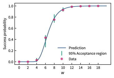
Figure 1: Probability of success of the Radical Attack given the “excess width” $w$ of the matrix $(\mathbf{B}\,|\,\mathbf{C})$. The solid sigmoidal curve is the simplified theoretical estimate $\operatorname{Prob}[\text{success}\,|\,w]\approx(1-2^{-w})^{g+m-n}$. Red dots represent empirical success probabilities for all values of $w$ for which failures have been observed during 100k numerical runs. Each vertical bar is the acceptance region of a test for compatibility with the theory prediction at significance level $\alpha=5\%$. The plot is truncated at $w=18$, as this is the largest value for which RadicalAttack$()$ has failed at least once to recover the correct secret in the experiment. The mean value of $w$ is about $32.3$ and more than 96% of all instances were associated with a value of $w$ exceeding 18. The simplified theoretical analysis reproduces the behavior of the algorithm in a quantitatively correct way, including predicting the transition from likely failure to likely success at around $w\approx 6$.

We have sampled $\gtrapprox$ 100k instances of $\mathbf{H}$ for $m=360,n=300,g=4$; see [29] for computer code and the raw data. Only in 154 cases did the Radical Attack fail to uncover the secret.

Given the number of approximations made, the theoretical analysis turns out to give a surprisingly accurate quantitative account of the behavior of the attack. This is visualized in Fig. 1. In particular, the transition from expected failure to expected success around $w_{\frac{1}{2}}\simeq 6.3$ can be clearly seen in the data. Consistent with the theory, no failures were observed for instances with $w>18$.

4.2.1 Uncertainty quantification for the numerical experiments

Because many of the predicted probabilities are close to $0$ or $1$, finding a suitable method of uncertainty quantification is not completely trivial.

Commonly, when empirical findings in the sciences are compared to theoretical predictions, one computes a confidence interval with coverage probability $(1-\alpha)$ for the estimated quantity and checks whether the theory prediction lies within that interval. Operationally, this furnishes a statistical hypothesis test for the compatibility between data and theory at significance level $\alpha$ (i.e. the probability that this method will reject data that is in fact compatible is at most $\alpha$). However, among the set of all hypothesis tests at a given significance level, some are more powerful than others, in the sense that they reject more data sets. The common method just sketched turns out to be of particularly low power in our setting.

Indeed, consider the extreme case where the hypothesis is $X\sim\operatorname{Binom}(N,p=0)$. Then a single instance of a non-zero outcome $X_{i}=1$ is enough to refute the hypothesis at any significance level. In other words, the acceptance region for the empirical probability $\hat{p}=|\{i\,|\,X_{i}=1\}|/N$ is just $\{0\}$. On the other hand, the statistical rule of three states that if no successes have been observed in $N$ attempts, a $95\%$-confidence region needs to have size about $3/N$.

Happily, for testing compatibility with the predicted parameter of a binomial distribution, there is a uniformly most powerful unbiased (UMPU) test [30, Chapter 6.2]. The vertical bars in Fig. 1 represent the resulting acceptance region. We re-iterate that this test is much more stringent than the more common approach based on confidence intervals would be.

4.3 The challenge data set

In light of the very high success rate observed on randomly drawn examples, it came as a surprise to us that an initial version of our attack failed for the challenge data set that the authors provided in Ref. [24]. Fortunately, Bremner, Cheng, and Ji were kind enough to publish the full version control history of their code [24]. The challenge was added with commit d485f9. Later, commit 930fc0 introduced a bug fix in the row redundancy routine. Under the earlier version, there was a high probability of the $\operatorname{range}(\mathbf{B}\,|\,\mathbf{C})=\mathbbm{F}_{2}^{m_{2}}$-condition failing. In this case, elements of $\ker\mathbf{G}$ would not necessarily correspond to elements of the radical. However, in the challenge data set, the doubly even part of $\mathbf{H}(\ker\mathbf{G})$ is contained in the radical. A minimalist fix—removing all singly-even columns from the generator matrix for $\mathbf{H}(\ker\mathbf{G})$—suffices to recover the hidden parameters:

$$g=4,\quad d=35,\quad m_{1}=96,$$

and the secret

$\mathbf{s}=$ cyCxfXKxLxXu3YWND2fSzf+YKtZJFLWY1J0l2rBao0A5zVWRSKA=

given here as a base64-encoded binary number. The string has since been kindly confirmed as being equal to the original secret by Michael Bremner, Bin Cheng, and Zhengfeng Ji.

4.4 Application to the Extended Quadratic Residue Code construction

The Radical Attack performs even better against the QRC construction with parameters

$$q\in\{103,127,151,167,223\},\quad r=\frac{q+1}{2},\quad m=2q,\quad n=r+q$$

recommended by Bremner, Cheng, and Ji as most resilient against the Kahanamoku-Meyer approach, see Section 3.3. In 20k runs we have found not a single instance in which the Radical Attack fails for these parameter choices; see Ref. [29] for code and raw data.

The Extended QRC construction does not fix $n$ to $r+q$, but rather allows for all values between $r$ and $q+r$. This raises the possibility that there is a parameter regime in which both the Linearity Attack and the Radical Attack fail. In Fig. 2 we explore this possibility. We find that the Radical Attack succeeds with high probability for $n\gtrsim q+13$. As discussed after Corollary 3, this matches the regime in which we expect

1. the rank of the added row redundancy to saturate such that the condition $\operatorname{range}(\mathbf{B}|\mathbf{C})=\mathbbm{F}_{2}^{m_{2}}$ of Corollary 3 is satisfied, and

2. the parameter $w=n-q-1$ to exceed $\log_{2}m_{1}=\log_{2}q$, which for the choices of $q=103,127,151,167$ is given by $\log_{2}q\approx 7$.

Let us also note that the QRC code is guaranteed to have the $\mathbf{1}_{[m_{1}]}=\mathbf{1}_{[q]}$ vector as a codeword and hence, it is guaranteed to have full support on the obfuscated coordinates.

Comparing this performance with the Linearity Attack, we find only a very slim region around $n\approx q+13$ in which there exist instances that cannot be solved by either attack with near-certainty. This motivates the exploration of further cryptanalytic approaches in Section 5, where we will indeed present two algorithms—the Lazy Linearity Attack and the Double Meyer, both building on the appproach of Kahanamoku-Meyer [22]—that will eliminate the remaining gap.

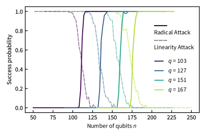
Figure 2: Performance of the Radical Attack and the Linearity Attack [22] on the updated QRC construction of Bremner, Cheng, and Ji [23], using 100 random instances per point. Linearity Attack data from [23, Fig. 3b]. The two approaches are seen to complement each other almost perfectly.

5 Further Attacks

The Stabilizer IQP Scheme features a large number of degrees of freedom that may allow an algorithm designer to evade any given exploit. The purpose of this section is to exhibit a variety of further approaches that might aid the cryptanalysis of obfuscated IQP circuits. Because the goal is to give an attacker a wide set of tools that may be adapted to any particular future construction, we focus on breadth and, as compared to Sec. 4, put less emphasis on rigorous arguments.

5.1 The Lazy Linearity Attack

We begin by slightly extending the Linearity Attack to what we call the Lazy Linearity Attack, summarized in Algorithm 2. In addition to the IQP tableau $\mathbf{H}$, this routine requires additional input parameters which we call the ambition $A$, the endurance $E$, and the significance threshold $g_{\text{th}}$.

Algorithm 2 Lazy Linearity Attack

1:function LazyLinearityAttack($\mathbf{H},g_{\text{th}},A,E$)

2:     while $\epsilon<E$ do

3:         Draw a uniformly random $\mathbf{d}\leftarrow\mathbbm{F}_{2}^{n}$

4:         $\mathbf{G}_{\mathbf{d}}\leftarrow\mathbf{H}_{\mathbf{d}}^{T}\mathbf{H}_{\mathbf{d}}$

5:         if $\dim\ker\mathbf{G}_{\mathbf{d}}<A$ then

6:              for $\mathbf{x}\in\ker\mathbf{G}_{\mathbf{d}}$ do

7:                  if $\operatorname{rad}\operatorname{range}(\mathbf{H}_{\mathbf{x}})\neq\{0\}$ and doubly-even and $\operatorname{rank}(\mathbf{H}_{\mathbf{x}}^{T}\mathbf{H}_{\mathbf{x}})\leq g_{\text{th}}$ then

8:                       return $\mathbf{x}$ and exit.

9:                  end if

10:              end for

11:         end if

12:         $\epsilon\leftarrow\epsilon+1$

13:     end while

14:     return “fail”

15:end function

5.1.1 Analysis

We start by briefly recapitulating why the Linearity Attack of Kahanamoku-Meyer [22] is effective. Essentially, it is based on the following property of the kernel of the Gram matrix $\mathbf{G}_{\mathbf{d}}$ for vectors $\mathbf{d}\in\mathbbm{F}_{2}^{n}$.

Lemma 5.

For $\mathbf{d}\in\mathbbm{F}_{2}^{n}$, let $\mathbf{G}_{\mathbf{d}}\coloneqq\mathbf{H}_{\mathbf{d}}^{T}\mathbf{H}_{\mathbf{d}}$. The following implication is true

$$\mathbf{H}_{s}\mathbf{d}\in\operatorname{rad}\mathcal{C}_{s}\quad\Rightarrow\quad\mathbf{s}\in\ker(\mathbf{G}_{\mathbf{d}}).$$ (15)

Proof.

By definition, it holds that $\mathbf{H}_{s}\mathbf{d}\in\operatorname{rad}\mathcal{C}_{s}$ iff

$$\mathbf{d}^{T}\mathbf{H}_{s}^{T}\mathbf{H}_{s}\mathbf{e}=\mathbf{d}^{T}\mathbf{H}^{T}\mathbf{H}_{s}\mathbf{e}=0\qquad\forall\,\mathbf{e}\in\mathbbm{F}_{2}^{n}.$$ (16)

Because $\mathbf{s}\mapsto\mathbf{H}_{\mathbf{s}}$ is linear, the above means that every element $\mathbf{H}{\mathbf{d}}\in\operatorname{rad}\mathcal{C}_{s}$ of the radical gives rise to a set of linear equations (one for each $\mathbf{e}\in\mathbbm{F}_{2}^{n}$) for the secret $\mathbf{s}$. These equations can be compactly written as

$$\mathbf{d}^{T}\mathbf{H}^{T}\mathbf{H}_{s}=0\quad\Leftrightarrow\quad\mathbf{H}^{T}\mathbf{H}_{\mathbf{d}}\mathbf{s}=0\quad\Leftrightarrow\quad\mathbf{H}_{\mathbf{d}}^{T}\mathbf{H}_{\mathbf{d}}\mathbf{s}=0.$$ (17)

∎

In the Linearity Attack, the strategy is now to pick $\mathbf{d}$ at random. Then with probability

$$\frac{|\operatorname{rad}\mathcal{C}_{\mathbf{s}}|}{|\mathcal{C}_{\mathbf{s}}|}=\frac{2^{\dim\operatorname{rad}\mathcal{C}_{\mathbf{s}}}}{2^{\dim\mathcal{C}_{\mathbf{s}}}}=2^{-g},$$ (18)

$\mathbf{d}$ lies in the radical of $\mathcal{C}_{\mathbf{s}}$ and we get a constraint on $\mathbf{s}$. If the kernel of $\mathbf{G}_{\mathbf{d}}$ is typically small, one can iterate through all candidates for $\mathcal{C}_{\mathbf{s}}$ and check the properties of the true $\mathcal{C}_{\mathbf{s}}$, namely, that $\operatorname{rad}\mathcal{C}_{\mathbf{s}}$ is doubly even and that its is given by $g$.

Since the rows of $\mathbf{H}$ are essentially random, we expect that $\mathbf{H}_{\mathbf{d}}$ has around $m/2$ rows which are linearly independent. In the original scheme of Shepherd and Bremner [19], $n\simeq m/2$, and we thus expect $\dim\ker(\mathbf{G}_{\mathbf{d}})\in O(1)$. More precisely, Bremner, Cheng, and Ji show that indeed $\mathbb{E}_{\mathbf{d}}[\dim\ker\mathbf{G}_{\mathbf{d}}]\geq n-m/2$. Thus, the runtime of the Linearity Attack scales exponentially with $n-m/2$. In the new challenge of Bremner, Cheng, and Ji, $n=300,m=360$, so that $n-m/2=120$, meaning that $\ker\mathbf{G}_{\mathbf{d}}$ is so large that this simple approach is no longer feasible.

In fact, for $n-m/2>0$, already the kernel of $\mathbf{H}_{\mathbf{d}}$ (which is contained in $\ker\mathbf{G}_{\mathbf{d}}$) will be nontrivial. But the relevant part of the kernel of $\mathbf{G}_{\mathbf{d}}$ in which the secret is hiding is independent of $n$ so long as $g+d<n$, and only requires that $\mathbf{d}$ has zero-entries in the obfuscated coordinates of $\mathbf{F}$. Thus, we expect that $\dim\ker\mathbf{G}_{\mathbf{d}}$ is roughly independent of the event $\mathbf{s}\in\ker\mathbf{G}_{\mathbf{d}}$. We can thus allow ourselves to ignore large kernels in the search for $\mathbf{s}$, if we are less ambitious about exploring those very large kernels, boosting the success probability.

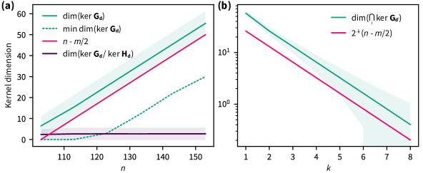
Figure 3: (a) Dimension of $\ker(\mathbf{G}_{\mathbf{d}})$ (green) for the QRC construction with $q=103$ and $m=2q$ for 100 random instances and 1000 random choices of $\mathbf{d}$ per point. Shaded areas represent one standard deviation. This is compared to the simplified theoretical prediction $n-m/2$ (pink). The dotted line designates the minimum observed value of $\dim(\ker\mathbf{G}_{\mathbf{d}})$. The original Linear Attack runs in time roughly exponential in the green curve, whereas the “lazy” approach reduces this to about the exponential of the dotted one. Finally, the violet line depicts $\ker(\mathbf{G}_{\mathbf{d}})/\ker(\mathbf{H}_{\mathbf{d}})$. The fact that it does not depend on $n$ is compatible with the expectation that the probability of finding the secret $\mathbf{s}$ in the kernel of any given Gram matrix $\mathbf{G}_{\mathbf{d}}$ is roughly independent of the size of the kernel.
(b) Dimension of $\bigcap_{i\in[k]}\ker(\mathbf{G}_{\mathbf{d}^{i}})$ (green) for the QRC construction with $q=103,n=q+r,r=(q+1)/2,m=2q$. We used 100 random instances and 1000 random choices of $\mathbf{d}^{1},\ldots,\mathbf{d}^{k}$ per point. The simple theoretical prediction of $2^{-k}(n-m/2)$ (pink) is seen to be in good agreement with the numerical experiments up to a constant prefactor.

More precisely, we expect that $\langle\mathbf{H}_{i},\mathbf{d}\rangle=1$ with probability $1/2$. Thus, the number of rows $m_{\mathbf{d}}$ of $\mathbf{H}_{\mathbf{d}}$ will follow a binomial distribution

$$m_{\mathbf{d}}\sim\operatorname{Bin}\left(N\approx m,p=0.5\right),$$ (19)

with mean $m/2$ and standard deviation $\sqrt{m}/2$. Sincemost rows of $\mathbf{H}$ are linearly independent and we expect the values of $\langle\mathbf{H}_{i},\mathbf{d}\rangle$ to be only weakly correlated, we thus expect the dimension of the kernel to be given by $\dim(\ker\mathbf{H}_{\mathbf{d}})\approx n-m_{\mathbf{d}}$ which is roughly Gaussian around $n-m/2$ with standard deviation $\sqrt{m}/2$; see [25, Theorem 3.2.2] for a more precise statement.

For the Lazy Linearity Attack the relevant parameter determining the success of the attack is the probability of observing a small kernel in the tail of the distribution over kernels of $\mathbf{H}_{\mathbf{d}}$, induced by the random choice of $\mathbf{d}$. As discussed above, this probability decreases exponentially with $n-m/2=g+w+i$, where we have defined the imbalance

$$i\coloneqq\frac{m_{2}-m_{1}}{2}.$$ (20)

Let the cumulative distribution function of the Gaussian distribution with mean $\mu$ and standard deviation $\sigma$ be given by $C_{\mu,\sigma}:\mathbb{R}\rightarrow[0,1]$. Then, the expected endurance required for the Lazy Linearity Attack with ambition $A$ to succeed is given by

$$E\sim\frac{2^{g}}{C_{n-m/2,\sqrt{m}/2}(A)}.$$ (21)

In numerical experiments, we find our predictions to be accurate up to a constant offset in the predicted mean of $\dim(\ker\mathbf{H})$, see Fig. 3a. In particular, the dimension of $\ker\mathbf{G}/\ker\mathbf{H}$ is independent of $n$, which is indeed evidence that there is no correlation between the size of the kernel of $\mathbf{G}$ and whether or not it contains a secret.

5.1.2 Application to the Extended QRC construction

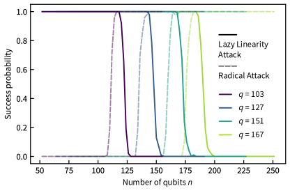
Figure 4: Performance of the Lazy Linearity Attack (solid lines) with ambition $A=8$, endurance $E=1000$, and significance threshold $g_{\text{th}}=1$, and the Radical Attack (dashed lines) for values of $q=103,127,151,167$. $100$ instances per point. Compared to Fig. 2, we find that the “lazy” approach has extended the range of $n$ for which the Linear Attack recovers the secret with near-certainty. The shift is sufficient that the two algorithms now cover the entire parameter range.

Applying the Lazy Linearity Attack to the Extended QRC construction, we find that it succeeds with near-unit success rate until $n-m/2\sim 10$ with parameters $A=8,E=1000$. Combined with the Radical Attack, we are now able to retrieve the secrets for all proposed parameters of the Extended QRC construction, see Fig. 4. For the Extended QRC construction, $m_{1}=m_{2}$, which means that $i=0$, and hence the success probability of the Lazy Linearity Attack decreases exactly with $w+g$ and the tunable parameters of the method.

5.2 The Double Meyer Attack

In the previous section, we discussed how to exploit statistical fluctuations to avoid having to search through large kernels. As $m-n/2$ increases, this strategy will fail to be effective. We thus present another ansatz, the Double Meyer Attack, stated as Algorithm 3. It reduces the size of the kernel, essentially by running several Linearity Attacks at once.

Algorithm 3 Double Meyer Attack

1:function DoubleMeyer($\mathbf{H},k,g_{\text{th}},A,E$)

2:     while $\epsilon<E$ do

3:         for $i\in[k]$ do

4:              Draw a uniformly random $\mathbf{d}^{i}\leftarrow\mathbbm{F}_{2}^{n}$

5:              $\mathbf{G}_{\mathbf{d}^{i}}\leftarrow\mathbf{H}_{\mathbf{d}^{i}}^{T}\mathbf{H}_{\mathbf{d}^{i}}$

6:              $\mathbf{G}\leftarrow(\mathbf{G}^{T}|\mathbf{G}_{\mathbf{d}^{i}}^{T})^{T}$

7:         end for

8:         if $\dim\ker\mathbf{G}<A$ then

9:              for $\mathbf{x}\in\ker\mathbf{G}_{\mathbf{d}}$ do

10:                  if $\operatorname{rad}\operatorname{range}(\mathbf{H}_{\mathbf{x}})\neq\{0\}$ and doubly-even and $\operatorname{rank}(\mathbf{H}_{\mathbf{x}}^{T}\mathbf{H}_{\mathbf{x}})\leq g_{\text{th}}$ then

11:                       return $\mathbf{x}$ and exit.

12:                  end if

13:              end for

14:         end if

15:         $\epsilon\leftarrow\epsilon+1$

16:     end while

17:     return “fail”

18:end function

5.2.1 Analysis

At a high-level, the Double Meyer Attack examines the elements of the intersection of the kernels of several $\mathbf{G}_{\mathbf{d}^{i}}$, where the $\mathbf{d}^{i}$ are uniformly distributed random vectors. Since the events $\mathbf{H}_{\mathbf{s}}\mathbf{d}^{i}\in\operatorname{rad}\mathcal{C}_{s}$ are independent for different $i$’s, we have that

$$\Pr\left[\mathbf{s}\in\bigcap_{i\in[k]}\ker\mathbf{G}_{\mathbf{d}^{i}}\right]=(2^{-g})^{k}=2^{-gk}.$$ (22)

At the same time, $\dim(\bigcap_{i\in[k]}\ker\mathbf{G}_{\mathbf{d}^{i}})\approx 2^{-k}(m-n/2)$, a behavior suggested by the fact that any given row of $\mathbf{H}$ will have non-zero inner product with all the $\mathbf{d}^{i}$ with probability $2^{-k}$.

Choosing $k\sim\log n$ is sufficient to reduce the kernel dimension to $O(1)$. Moreover, $g$ needs to be of order $O(\log n)$ in order to maintain a sample-efficient verification test for the challenge. Thus, $2^{gk}\in 2^{O(\log^{2}(n))}$, i.e. the Double Meyer Attack is expected to run in at most most quasi-polynomial time, for any choice of $n,m$. However, even moderate values of $g$ will make this approach infeasible in practice. For the challenge data set, we expect that good parameter choices are $k=6$, $A=3$ and $E\gtrsim 2^{gk}=2^{24}\approx 10^{7.22}$, though we have not spent enough computational resources to have recovered a secret in this regime.

We observe that slack between the threshold rank $g_{\text{th}}$ and the true $g$ often leads to a misidentified secret. This is explained by vectors $\mathbf{v}\in\bigcap_{i\in[k]}\ker\mathbf{H}_{\mathbf{d}^{i}}$ whose image under $\mathbf{H}$ has low Hamming weight $|\mathbf{H}\mathbf{v}|\leq g_{\text{th}}-g$. This corresponds to rows of $\mathbf{H}$ which can be mapped to $s=g_{\text{th}}-g$ unit vectors $\mathbf{e}^{1},\ldots,\mathbf{e}^{s}$ which are linearly independent of the first $m_{1}$ rows of $\mathbf{H}$. These vectors may be absorbed into $\mathbf{F}$, adding $s$ nontrivial columns to it, while adding a zero row to $\mathbf{D}$, which keeps its range doubly even. The alternative secrets $\mathbf{v}$ found in this way are also observable in the sense that they satisfy $\Pr_{\mathbf{x}\leftarrow D_{\mathbf{H}}}[\langle\mathbf{x},\mathbf{v}\rangle=0]=(2^{-(g+s)/2}+1)/2$. In order to find the “true” secret, one should therefore run the attack for increasing values of $g_{\text{th}}$, and halt as soon as a valid secret is found.

The low-Hamming weight vectors identified above inform the final ansatz of this paper, Hamming’s Razor, presented in Section 5.3.

5.2.2 Application to the Extended QRC construction

We find that the Double Meyer Attack recovers the secrets of the Extended QRC construction with near-certainty in all parameter regimes proposed by Bremner, Cheng, and Ji. For the QRC construction, $g=1$ and hence the runtime of the Double Meyer Attack is just given by $2^{k}$. Choosing $k=6,g_{\text{th}}=1,E=8,A=1000$ is sufficient to recover the secret in all of $100$ random instances of the Extended QRC construction for all values of $n\in[r,q+r]$ and $q\in\{103,127,151,167\}$.

5.3 Hamming’s Razor

In this section, we describe a method that allows one to “shave off” certain rows and columns from $\mathbf{H}$ without affecting the code space $\mathcal{C}_{\mathbf{s}}$. Such redundancies can be identified given a vector $\mathbf{d}\in\mathbbm{F}_{2}^{n}$ such that $\mathbf{H}\mathbf{d}$ has low Hamming weight. The method comes in two varieties: The simpler Singleton Razor, discussed first, and the more general Hamming’s Razor.

5.3.1 The Singleton Razor

Let us agree to call $i\in[m]$ a singleton for $\mathbf{H}$ if there is a solution to $\mathbf{H}\mathbf{d}=\mathbf{e}^{i}$.

We discuss the idea based on the unobfuscated picture of Eq. 3. Assume that $\operatorname{supp}\operatorname{range}\mathbf{D}=[m_{1}]$. Then there is no singleton among the first $m_{1}$ coordinates, because $\mathbf{e}^{i}$ is not orthogonal to $\operatorname{range}\mathbf{D}$, while all vectors in the range of $(\mathbf{F}\,|\,\mathbf{D})$ are. Thus, knowing a singleton $i$, one may trim away the $i$-th row of $\mathbf{H}$ without affecting the code space. Alternatively, one can perform a coordinate change on $\mathbbm{F}_{2}^{n}$ that maps the corresponding pre-image $\mathbf{d}$ to $\mathbf{e}^{n}$ and then drop the $n$-th column of $\mathbf{H}$. In fact, both operations may be combined, without changing $\mathcal{C}_{\mathbf{s}}$.

The generator matrix $\mathbf{H}$ of the challenge data set affords $69$ singletons. All singletons do indeed belong to redundant rows [29]. The second part of Lemma 6 below suggests an explanation for this surprisingly high number.

5.3.2 Hamming’s Razor

We now generalize the singleton idea to higher Hamming weights. Starting point is the observation that $\operatorname{range}\mathbf{C}$ can be expected to contain vectors of much lower Hamming weight than $\operatorname{range}\mathbf{(}\mathbf{F}\,|\,\mathbf{D})$. This will lead to a computationally efficient means for separating redundant from non-redundant rows.

The following lemma collects two technical preparations.

Lemma 6.

Let $\mathbf{M}$ be an $m\times(m-h)$ binary matrix chosen uniformly at random. The probability that the minimal Hamming weight of any non-zero vector in the range of $\mathbf{M}$ is smaller than $k$ is exponentially small in $k_{1}-k$, where

$$k_{1}=h\frac{\ln 2}{\ln m+2}\approx\frac{h}{\log_{2}m}.$$

More precisely and more strongly, the probability is no larger than $e^{-\lambda(k_{\infty}-k)}$, for

$$k_{\infty}=\lim_{i\to\infty}k_{i},\qquad k_{i}=k_{1}+\frac{(k_{i-1}-1)\ln k_{i-1}}{\ln m+2},\qquad\lambda=\frac{1}{k_{\infty}}+\ln\frac{m}{k_{\infty}}>0.$$ (23)

Conversely, let $\mathbf{M}$ be any binary matrix whose range has co-dimension $h$. For $S\subset[m]$, let $V_{S}\subset\mathbbm{F}_{2}^{m}$ be the subspace of vectors supported on $S$. Then $\operatorname{range}M$ has a non-trivial intersection with $V_{S}$ if $|S|>h$.

Proof.

Let $\mathbf{v}$ be a random vector distributed uniformly in $\mathbbm{F}_{2}^{m}$. Then, as long as $k\leq m/2$,

$$\Pr\left[|\mathbf{v}|\leq k\right]=\sum_{k^{\prime}\leq k}\binom{m}{k^{\prime}}2^{-m}\leq k\binom{m}{k}2^{-m}\quad\Rightarrow\quad\Pr\left[\min_{0\neq\mathbf{v}\in\operatorname{range}\mathbf{M}}|\mathbf{v}|\leq k\right]\leq k\binom{m}{k}2^{-h}.$$

Using the standard estimate $\ln\binom{m}{k}\leq k(\ln m+1)-k\ln k$, the logarithm of the bound is

$$l(k):=k(\ln m+1)-(k-1)\ln k-h\ln 2.$$

The function $l(k)$ is concave, negative at $k=0$, positive at $k=m/2$, and thus has a zero in the interval $[0,m/2]$. What is more, $l(k)=0$ if and only if

$$k=h\frac{\ln 2}{\ln m+1}+\frac{(k-1)\ln k}{\ln m+1}.$$

Because the r.h.s. is monotonous in $k$, the recursive formula (23) defines an increasing sequence $k_{i}$ of lower bounds to the first zero. As a non-decreasing sequence on a bounded set, the limit point $k_{\infty}$ is well-defined. Due to concavity, $l(k)$ is upper-bounded by its first-order Taylor approximations. The claim then follows by expanding around $k=k_{\infty}$.

The converse statement is a consequence of the standard estimate

$$\dim\big{(}\operatorname{range}\mathbf{M}\cap V_{S})\geq\dim\operatorname{range}\mathbf{M}+\dim V_{S}-m.$$

∎

Choose a set $S\subset[m]$ and let $\mathbf{H}_{\setminus S}$ be the matrix obtained by deleting all rows of $\mathbf{H}$ whose index appears in $S$. Let $S_{1}=S\cap[m_{1}]$ be the intersection of $S$ with the “secret rows” and $S_{2}=S\cap[m_{1}+1,m_{2}]$ the intersection with the redundant rows. Then $\mathbf{d}\in\ker\mathbf{H}_{\setminus S}$ if and only if

$$\operatorname{supp}(\mathbf{H}_{\mathbf{s}}\mathbf{d})\subset S_{1}\quad\text{and}\quad\operatorname{supp}(\mathbf{R}_{\mathbf{s}}\mathbf{d})\subset S_{2}.$$

Now model $(\mathbf{F}\,|\,\mathbf{D})$ as a uniformly random matrix. Lemma 6 applies with $m=m_{1},h=m_{1}-g-d$, giving rise to an associated value of $k_{\infty}$. If $|S_{1}|<k_{\infty}$ then, up to an exponentially small probability of failure, the first condition can be satisfied only if $\mathbf{H}_{\mathbf{s}}\mathbf{d}=0$. Therefore, each non-zero element $\mathbf{d}\in\ker\mathbf{H}_{\setminus S}$ identifies $\operatorname{supp}(\mathbf{H}\mathbf{d})$ as a set of redundant rows, which can be eliminated as argued in the context of the Singleton Attack.

This observation is useful only if it is easily possible to identify suitable sets $S$ and non-zero vectors $\mathbf{d}$ in the associated kernel. Here, the second part of Lemma 6 comes into play. If $|S_{2}|>m_{2}-(n-g-d)$, then by the lemma and Eq. 8, there exists a non-zero $\mathbf{d}$ such that $\operatorname{supp}(\mathbf{C}\mathbf{d})\subset S_{2}$.

This suggests to choose $S$ by including each coordinate $i\in[m]$ with probability $p$ such that $pm_{2}>m_{2}-(n-g-d)$ and $pm_{1}<k_{\infty}$. For the challenge parameters, these requirements are compatible with the range $[0.01,0.13]$ for $p$.

In fact, one can base a full secret extraction method on this idea, see Algorithm 4. Repeating the procedure for a few dozen random $S$ turns out to reveal the entire redundant row set, and thus the secret, for the challenge data [29]. The attack may be sped up by realizing that the condition on $|S_{1}|$ was chosen conservatively. The first part of Lemma 6 states that the smallest Hamming weight that occurs in the range of $\mathbf{H}_{\mathbf{s}}$ is about $k_{\infty}$. But a randomly chosen $S_{1}$ of size larger than $k_{\infty}$ is unlikely to be the support of a vector in $\operatorname{range}\mathbf{H}_{\mathbf{s}}$ unless $|S_{1}|$ gets close to the much larger second bound in the lemma. This optimization, for a heuristically chosen value of $p=0.25$, is used in the sample implementation provided with this paper [29] and recovers the secret with high probability.

Algorithm 4 Hamming’s Razor

1:function HammingRazor($\mathbf{H},p,E$)

2:     $S\leftarrow\emptyset$.

3:     for $\_\in[E]$ do

4:         Draw a random vector $\mathbf{d}\in\mathbbm{F}_{2}^{m}$ with entries $\mathbf{d}_{i}\leftarrow\operatorname{Bin}(\mathbbm{F}_{2},p)$.

5:         $\mathbf{H}[\mathbf{d}]\leftarrow\operatorname{diag}(\mathbf{d})\mathbf{H}$.

6:         $\mathbf{K}\leftarrow$ a column-generating matrix for $\ker\mathbf{H}[\mathbf{d}]$.

7:         Append the support of the columns of $\mathbf{H}\mathbf{K}$ to $S$.

8:     end for

9:     Solve the $\mathbbm{F}_{2}$-linear system $\mathbf{H}\mathbf{s}=\mathbf{1}_{S^{c}}$

10:     return $\mathbf{s}$

11:end function

6 Discussion

In this work, we have exhibited a number of approaches that can be used to recover secrets hidden in obfuscated IQP circuits.

We emphasize that, in our judgment, the problem of finding ways to efficiently certify the operation of near-term quantum computing devices is an important one, and the idea to use obfuscated quantum circuits remains appealing. More generally, results that exhibit weaknesses in published constructions should not cause the community to turn away, but should rather serve as sign posts guiding the way to more resilient schemes. It may be instructive to compare the situation to the more mature field of classical cryptography, which benefits from a large public record of cryptographic constructions and their cryptanalysis. New protocols can thus be designed to resist known exploits and be vetted against them. The well-documented story of differential cryptanalysis provides an instructive example.

We hope that the quantum information community will look at the present results in a similarly constructive spirit.

Appendix A Implementation details

While running the software package provided with [23] tens of thousands of times, we found a number of extremely rare edge cases that were not explicitly handled.

In particular, the sample_parameters() and the sample_D() functions would very rarely return inconsistent results. Rather straight-forward corrections are published in [29].

Another possible discrepancy between the procedure described in the main text of Ref. [23] and their software implementation concerns the generation of the “redundant rows”. The issue is a little more subtle than the first two, so we briefly comment on it here.

In the paper, the relevant quote is

“Therefore, up to row permutations, the first $n-r$ rows of $\mathbf{R}_{\mathbf{s}}$ are sampled to be random independent rows that are orthogonal to $\mathbf{s}$ and lie outside the row space of $\mathbf{H}_{\mathbf{s}}$.”

(emphasis ours). The computer implementation is given by the add_row_redundancy() function in lib/construction.py, in particular by these lines:

s_null_space = s.reshape((1, -1)).null_space()

full_basis = row_space_H_s
for p in s_null_space:
  if not check_element(full_basis.T, p):
  full_basis = np.concatenate((full_basis, p.reshape(1, -1)), axis=0)

R_s = full_basis[r:] # guarantee that rank(H) = n

At this point, the first $n-r$ rows of $R_{s}$ are not “random independent”. The behavior of this piece of code depends on the detailed implementation of the null_space() function, which we do not directly control. While the obfuscation process will later add randomness, we caution that the same random invertible matrix $\mathbf{Q}$ acts both on $\mathbf{R}_{\mathbf{s}}$ and on $\mathbf{H}_{\mathbf{s}}$. Any relation between these two blocks that is invariant under right-multiplication by an invertible matrix will therefore be preserved. As a mitigation of this possible effect, we suggest to add an explicit randomization step, such as

Ψs_null_space=rand_inv_mat(s_null_space.shape[0],seed=rng)@s_null_space

to the routine. (Though in practice, we did not observe different behavior between these two versions).

The code published in [29] contains three implementations of the add_row_redundancy() function. The version used to create the challenge data (c.f. Sec. 4.3), the one published with Ref. [23], and finally the one with the explicit extra randomization step added. The numerical results reported in the main part of this paper were generated by the third routine, though we have also include 20k runs performed with the second version [29]. The effectiveness of the Radical Attack does not seem to differ appreciatively between these two implementations.

References

- Gidney and Ekerå [2021] C. Gidney and M. Ekerå, Quantum 5, 433 (2021).
- Litinski [2023] D. Litinski, (2023), arXiv:2306.08585 .
- Brakerski et al. [2018] Z. Brakerski, P. Christiano, U. Mahadev, U. Vazirani, and T. Vidick, in 2018 IEEE 59th Annual Symposium on Foundations of Computer Science (FOCS) (2018) pp. 320–331.
- Brakerski et al. [2020] Z. Brakerski, V. Koppula, U. Vazirani, and T. Vidick, (2020), arXiv:2005.04826 .
- Kahanamoku-Meyer et al. [2022] G. D. Kahanamoku-Meyer, S. Choi, U. V. Vazirani, and N. Y. Yao, Nat. Phys. 18, 918 (2022).
- Zhu et al. [2023] D. Zhu, G. D. Kahanamoku-Meyer, L. Lewis, C. Noel, O. Katz, B. Harraz, Q. Wang, A. Risinger, L. Feng, D. Biswas, L. Egan, A. Gheorghiu, Y. Nam, T. Vidick, U. Vazirani, N. Y. Yao, M. Cetina, and C. Monroe, Nat. Phys. 19, 1725 (2023), arXiv:2112.05156 .
- Bremner et al. [2010] M. J. Bremner, R. Jozsa, and D. J. Shepherd, Proceedings of the Royal Society A: Mathematical, Physical and Engineering Sciences 467, 459 (2010).
- Aaronson and Arkhipov [2013] S. Aaronson and A. Arkhipov, Th. Comp. 9, 143 (2013).
- Bremner et al. [2016] M. J. Bremner, A. Montanaro, and D. J. Shepherd, Physical Review Letters 117, 080501 (2016).
- Boixo et al. [2018] S. Boixo, S. V. Isakov, V. N. Smelyanskiy, R. Babbush, N. Ding, Z. Jiang, M. J. Bremner, J. M. Martinis, and H. Neven, Nature Phys 14, 595 (2018), arXiv:1608.00263 .
- Arute et al. [2019] F. Arute, K. Arya, R. Babbush, D. Bacon, J. C. Bardin, R. Barends, R. Biswas, S. Boixo, F. G. S. L. Brandao, D. A. Buell, and et al., Nature 574, 505 (2019).
- Zhong et al. [2020] H.-S. Zhong, H. Wang, Y.-H. Deng, M.-C. Chen, L.-C. Peng, Y.-H. Luo, J. Qin, D. Wu, X. Ding, Y. Hu, and et al., Science 370, 1460 (2020).
- Wu et al. [2021] Y. Wu, W.-S. Bao, S. Cao, F. Chen, M.-C. Chen, X. Chen, T.-H. Chung, H. Deng, Y. Du, D. Fan, and et al., Phys. Rev. Lett. 127, 180501 (2021).
- Pan et al. [2022] F. Pan, K. Chen, and P. Zhang, Phys. Rev. Lett. 129, 090502 (2022), arXiv:2111.03011 .
- Kalachev et al. [2021] G. Kalachev, P. Panteleev, P. Zhou, and M.-H. Yung, (2021), arXiv:2112.15083 .
- Morvan et al. [2023] A. Morvan, B. Villalonga, X. Mi, S. Mandrà, A. Bengtsson, P. V. Klimov, Z. Chen, S. Hong, C. Erickson, I. K. Drozdov, and et al., (2023), arXiv:2304.11119 .
- Hangleiter and Eisert [2023] D. Hangleiter and J. Eisert, Rev. Mod. Phys. 95, 035001 (2023), arXiv:2206.04079 .
- Yamakawa and Zhandry [2022] T. Yamakawa and M. Zhandry, (2022), arXiv:2204.02063 .
- Shepherd and Bremner [2009] D. Shepherd and M. J. Bremner, Proceedings of the Royal Society of London A: Mathematical, Physical and Engineering Sciences 465, 1413 (2009).
- Aaronson [2022] S. Aaronson, “Recent progress in quantum advantage,” (2022), talk at the Simons Institute; accessed 23/11/27.
- Aaronson [2023] S. Aaronson, “Verifiable quantum supremacy: What I hope will be done,” (2023), talk at the Simons Institute; accessed 23/11/27.
- Kahanamoku-Meyer [2023] G. D. Kahanamoku-Meyer, Quantum 7, 1107 (2023), arXiv:1912.05547 .
- Bremner et al. [2023a] M. J. Bremner, B. Cheng, and Z. Ji, (2023a), arXiv:2308.07152v1 .
- Bremner et al. [2023b] M. J. Bremner, B. Cheng, and Z. Ji, https://github.com/AlaricCheng/stabilizer_protocol_sim (2023b), commit 11d4c52.
- Kolchin [1998] V. F. Kolchin, Random Graphs, Encyclopedia of Mathematics and Its Applications (Cambridge University Press, Cambridge, 1998).
- Wood [1993] J. A. Wood, Trans. Amer. Math. Soc. 336, 445 (1993).
- Gross et al. [2021] D. Gross, S. Nezami, and M. Walter, Commun. Math. Phys. 385, 1325 (2021).
- Montealegre-Mora and Gross [2022] F. Montealegre-Mora and D. Gross, (2022), arXiv:2208.01688 .
- Gross and Hangleiter [2023] D. Gross and D. Hangleiter, “De-obfuscate IQP,” https://github.com/goliath-klein/deobfuscate-iqp (2023).
- Shao [2003] J. Shao, Mathematical Statistics, 2nd ed., Springer Texts in Statistics (Springer, New York, 2003).