Realizing Altermagnetism in Fermi-Hubbard Models with Ultracold Atoms

Abstract

Altermagnetism represents a new type of collinear magnetism distinct from ferromagnetism and conventional antiferromagnetism. In contrast to the latter, sublattices of opposite spin are related by spatial rotations and not only by translations and inversions. As a result, altermagnets have spin split bands leading to unique experimental signatures. Here, we show theoretically how a $d$-wave altermagnetic phase can be realized with ultracold fermionic atoms in optical lattices. We propose an altermagnetic Hubbard model with anisotropic next-nearest neighbor hopping and obtain the Hartree-Fock phase diagram. The altermagnetic phase separates in a metallic and an insulating phase and is robust over a large parameter regime. We show that one of the defining characteristics of altermagnetism, the anisotropic spin transport, can be probed with trap-expansion experiments.

Introduction.—Collinear quantum magnets are usually assumed to have either ferromagnetic or antiferromagnetic order [1, 2]. Ferromagnets break time-reversal symmetry leading to spin-split bands and a net polarization of the magnetic moment. Conventional antiferromagnets exhibit zero net magnetization and are symmetric under translation and spin-inversion, leading to spin-degenerate bands. However, recent studies have suggested refinements of this dichotomy and proposed a new class of collinear magnetism, that possess momentum dependent spin-split bands without net magnetization [3, 4, 5, 6, 7, 8] as recently confirmed experimentally in material candidates [9, 10, 11, 12]. These collinear states, dubbed altermagnets [7, 13], are characterized by additional rotational symmetries of the opposite spin sublattices. For example, in a $d$-wave altermagnet on the square lattice, sublattices are related by a spin flip followed by a $\pi/2$ real-space rotation about a point on the dual lattice; see Fig. 1 (a) for an illustration.

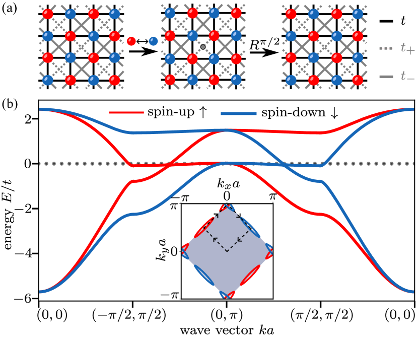
Figure 1: The altermagnetic Hubbard model. (a) A Néel state on an alternating anisotropic square lattice is a $d$-wave altermagnetic state. It is invariant under a global spin flip (exchanging red and blue dots) followed by a $\pi/2$ real-space rotation around the dual square lattice (gray dot). The nearest-neighbor hopping $t$ and the alternating diagonal hopping $t_{\pm}$ of the altermagnetic Hubbard model are indicated as well. (b) Spin-resolved band structure of the altermagnetic state at zero temperature for $t^{\prime}/t=0.3,\delta=0.9$, $U/t=3.5$ evaluated along the path indicated in the inset. Inset: Fermi surface and magnetic Brillouin zone (gray shaded area). The band structure obeys the symmetry shown in (a) and is therefore spin-split without net magnetization, which are the key characteristics of an altermagnet.

Over the recent years, exciting progress has been made in studying quantum magnetism with quantum simulators of ultracold atoms [14]. For the square lattice Hubbard model antiferromagnetic correlations of an extended range have been observed at the lowest experimentally accessible temperatures [15, 16, 17, 18] and the consequences of doping the antiferromagnetic state have been investigated [19, 20, 21, 22]. Frustrated triangular lattice Hubbard models have been started to be explored as well [23, 24, 25, 26]. Investigating the phenomena of altermagnetism with ultracold atoms remains an interesting open avenue.

In this work, we show how $d$-wave altermagnetism can be realized and characterized with ultracold atoms in optical lattices. We analyze a square lattice Hubbard model with uniform nearest-neighbor and alternating diagonal hoppings and show how this model can be realized by $45^{\circ}$ rotated optical lattices. Performing a Hartree-Fock analysis we find that this model stabilizes an altermagnetic phase in an extended parameter range and analyze the robustness of the state at finite temperatures. We demonstrate that the key experimental characteristic of the altermagnetic state, i.e., the anisotropic spin transport, can be measured by trap-expansion experiments.

The altermagnetic Hubbard model.—We consider two-species of fermionic atoms labelled by spin $s$ in an optical lattice described by the following altermagnetic Hubbard model

$$\hat{H}=-\sum_{i,j,s}t_{ij}(c_{is}^{\dagger}c_{js}+\text{h.c})+U\sum_{i}n_{i\uparrow}n_{i\downarrow},$$ (1)

where $U$ is the on-site Hubbard interaction and $t_{ij}$ the hopping matrix element, which is uniform and of strength $t$ for nearest neighbors, sublattice-dependent for diagonal neighbors, and zero otherwise. The diagonal hopping alternates with $t_{\pm}=t^{\prime}(1\pm\delta)$ as following: in the $(1,1)$-direction the hopping element is $t_{-}$ ($t_{+}$) and in the $(1,-1)$-direction it is $t_{+}$ ($t_{-}$) on the $A$ (B) sublattice, respectively; see Fig. 1 (a).

We consider half-filling $\langle n_{i}\rangle=\langle n_{i\uparrow}+n_{i\downarrow}\rangle=1$. However, our results remain qualitatively similar for small doping where the Néel order is stable. We will now show that this particular sublattice dependence of the diagonal hopping leads to altermagnetism and discuss later the optical lattice geometry required to realize this model.

In order to study the magnetic instabilities of our system, we perform a Hartree-Fock analysis that capturing the sublattice structure of the known $(\pi,\pi)$ magnetic instability. To this end, we introduce the order parameter $\delta m$ at filling $n$ as

$$\langle n_{r\lambda s}\rangle=n/2+\delta m(-1)^{\lambda+s},$$ (2)

where $r$ denotes the index of a unit cell, $\lambda$ the sublattice, and $s$ the spin. For the alternating sign of the order parameter $(-1)^{\lambda+s}$ we associate $\lambda$ and $s$ with 0 for A and $\uparrow$ and with 1 for B and $\downarrow$, respectively. Decoupling the interaction term and expressing it in terms of the mean-field order parameter leads after Fourier transformation to the effective interactions $-U\delta m\sum_{\bm{k}}(n_{\bm{k}A\uparrow}-n_{\bm{k}B\uparrow}-n_{\bm{k}A\downarrow}+n_{\bm{k}B\downarrow})$, where the wave vector $\bm{k}$ is in the magnetic Brillouin zone. The magnetic Brillouin zone is defined via the real space unit cell spanned by the primitive vectors $\bm{a}_{1}=a(1,1)$ and $\bm{a}_{2}=a(1,-1)$ with the lattice constant $a$ of the square lattice.

Expressing the mean-field Hamiltonian in the basis of $\Psi_{\bm{k}}^{\dagger}=(c_{{\bm{k}}A\uparrow}^{\dagger}c_{{\bm{k}}B\uparrow}^{\dagger}c_{{\bm{k}}A\downarrow}^{\dagger}c_{{\bm{k}}B\downarrow}^{\dagger})$, leads to

$$\begin{split}\hat{H}^{\text{HF}}=\sum_{\bm{k}}\Psi_{\bm{k}}^{\dagger}\vbox{\hbox{$\begin{bmatrix}H_{\uparrow}(\bm{k})&0\\ 0&H_{\downarrow}(\bm{k})\\ \end{bmatrix}$}}\Psi_{\bm{k}}.\end{split}$$ (3)

The Hamiltonian is block diagonal in the spin degree of freedom with $H_{s}(\bm{k})=\vbox{\hbox{$\begin{bmatrix}h_{AA,s}&h_{AB,s}\\ h_{BA,s}&h_{BB,s}\\ \end{bmatrix}$}}$, where $h_{AA,s}=-[2t_{-}\cos(\bm{k}\bm{a}_{1})+2t_{+}\cos(\bm{k}\bm{a}_{2})+(-1)^{s}U\delta m]$, $h_{BB,s}=-[2t_{+}\cos(\bm{k}\bm{a}_{1})+2t_{-}\cos(\bm{k}\bm{a}_{2})-(-1)^{s}U\delta m]$, $h_{AB,s}=-2t[\cos(k_{x}a)+\cos(k_{y}a)]$, and $h_{BA,s}=h_{AB,s}^{*}$. Due to the spin block-diagonal structure of the Hamiltonian (3), bands are fully spin-polarized. In addition, each of the spin components exhibit a momentum-inversion symmetry ($\bm{k}\to-\bm{k}$) and sublattices are staggered.

We solve the mean-field equations at finite temperatures $T$ by self-consistently determining the order parameter $\delta m=\frac{1}{4N}\sum_{\bm{k}}\langle n_{\bm{k}A\uparrow}-n_{\bm{k}B\uparrow}-n_{\bm{k}A\downarrow}+n_{\bm{k}B\downarrow}\rangle_{\text{HF}}$ as well as the chemical potential $\mu$, which is set by fixing the particle number; see supplemental materials for details [27]. We compute the spin-resolved band structure for $t^{\prime}/t=0.3,\delta=0.9$, and $U/t=3.5$ at half-filling $n=1$; see Fig. 1 (b). Both the band structure and the Fermi surface possess the altermagnetic symmetry of a $\pi/2$ rotation along with a spin-flip. Here, the reciprocal lattice vectors of the magnetic Brillouin zone are $\frac{\pi}{2a}(1,1)$ and $\frac{\pi}{2a}(1,-1)$; see shaded area in the inset of Fig.1 (b).

Figure 2: Robustness of altermagnetism. We compute the altermagnetic order parameter $\delta m$ as a function of interaction strength $U/t$ and diagonal hopping $t^{\prime}/t$ for staggering $\delta=0.2$ and temperatures (a) $T=0$ and (b) $T=0.2t$. The system is in a normal metallic state when the order parameter vanishes, while a finite order parameter indicates altermagnetic symmetry breaking. (c) Line cut along the dashed line in (a) shows the order parameter at zero temperature for $t^{\prime}/t=0.3$ and $\delta=0.2$. Three phases are distinguished: The normal metal (NM) at weak interactions, the altermagnetic metal (AMM) possessing a Fermi surface at intermediate interactions, and the gapped altermagnetic insulator (AMI) at strong interactions. Within the AMM the kink in the order parameter at $U/t\approx 2.5$ indicates a Lifshitz transition at which half of the Fermi pockets vanish.

Having established the altermagnetic state, we study its robustness by tuning the system parameters and the temperature. To this end, we compute the order parameter $\delta m$ as a function of $U/t$ and $t^{\prime}/t$ for $\delta=0.2$ and $T=0$ and $0.2t$ in Fig. 2 (a,b). We will show below that the hopping parameters can be controlled by the optical lattice. Moreover, the interaction $U$ is tunable by Feshbach resonances in ultracold atomic systems [28]. The altermagnetic phase is stabilized for increasing diagonal hopping $t^{\prime}$, staggering $\delta$, and interaction strength $U$. It can be either metallic, characterized by the presence of small Fermi surfaces, or a gapped insulator. A line cut though the phase diagram unveils phase transitions from a normal metal (NM) with vanishing $\delta m$ over an altermagnetic metal (AMM) to an altermagnetic insulator (AMI); see Fig. 2 (c). In addition, we find a kink in the order parameter $\delta m$ within the AMM at $U/t\approx 2.5$. This is a Lifshitz transition at which half of the Fermi pockets around $(\pm\pi/2a,\pm\pi/2a)$ disappear. The altermagnetic phase occupies a large portion of the phase diagram, because the underlying mechanism is a consequence of the symmetry of the single-particle band structure. The interactions are only required to establish Néel order, which splits the bands appropriately.

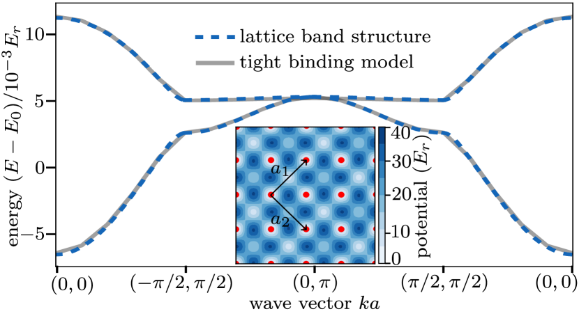
Figure 3: Effective band structure of the optical lattice. Lowest two bands, solid lines, obtained from solving the Schrd̈inger equation of a particle in an optical lattice potential with with $V_{0}=4E_{r},V_{1}/V_{0}=2.2$, and $\Delta=0.6$; see Eq. (4). Bands obtained from a tight-binding model with uniform nearest-neighbor hopping $t$ and the alternating diagonal hopping amplitudes $t_{\pm}=t^{\prime}(1\pm\delta)$, dashed line, agree well with the full band structure. The effective parameters of the tight-binding model are $t=2.2\times 10^{-3}E_{r},t^{\prime}/t=0.16,\delta=0.83$ and the energy offset is $E_{0}=13.81E_{r}$. Inset: Illustration of the optical lattice potential.

Optical lattice for the altermagnetic band structure.—The altermagnetic Hubbard model has uniform nearest-neighbor and alternating diagonal hopping elements. Such a single-particle band structure is realized when considering $45^{\circ}$-rotated counter-propagating and phase-locked lasers of wave length $\lambda$ and $2\lambda$ with different strengths, respectively. Specifically, we consider the following lattice potentials

$$\begin{split}V_{\text{latt}}&=E_{r}(V_{\text{sq}}+V_{d,1}+V_{d,2})\\ V_{\text{sq}}&=V_{0}[\sin^{2}(k_{l}x)+\sin^{2}(k_{l}y)]\\ V_{d,1}&=V_{1}\Big{[}\Delta_{+}\sin^{2}[k_{l}(x+y)]+\Delta_{-}\sin^{2}[\frac{k_{l}}{2}(x+y)]\Big{]}\\ V_{d,2}&=V_{1}\Big{[}\Delta_{+}\sin^{2}[k_{l}(x-y)]+\Delta_{-}\cos^{2}[\frac{k_{l}}{2}(x-y)]\Big{]},\end{split}$$ (4)

where $k_{l}=2\pi/\lambda$ is the lattice wave vector, $E_{r}=\frac{\hbar^{2}k_{l}^{2}}{2m}$ is the recoil energy, $m$ is the mass of the atoms, and $\Delta_{\pm}=(1\pm\Delta)$ the potential staggering of strength $\Delta$. The potential consists of deep minima on a square lattice and shallow minima on the dual lattice that are tuned by $V_{0}$, $V_{1}$, and $\Delta$; see inset of Fig. 3. For such an optical lattice both the nearest neighbor and the diagonal tunneling are sizeable.

The unit cell of the lattice is $\sqrt{2}a\times\sqrt{2}a$, where $a$ is the lattice constant of the square lattice, with primitive lattice vectors $\bm{a}_{1}$ and $\bm{a}_{2}$; see inset of Fig. 3. We numerically solve the Schrödinger equation of a single particle in this optical lattice potential by standard techniques (see e.g. Ref. 29) and show the lowest two bands in Fig. 3. We then fit the lowest bands to the tight-binding Hamiltonian of the altermagnetic Hubbard model and obtain the uniform nearest-neighbor hopping $t$ and the staggered diagonal hoppings $t_{\pm}=t^{\prime}(1\pm\delta)$. The diagonal hopping elements are sizeable for this lattice because of the potential minima at the dual lattice sites. The tight-binding band structure reproduces well the lowest two bands; Fig. 3. Here, we have considered deep optical lattices, leading to comparatively low absolute scales of the hopping. While giving rise to slightly more complex band structures, shallower lattices and hence larger absolute hopping scales will not alter our findings qualitatively. The tight-binding parameters are tunable by $V_{0}$, $V_{1}$, and $\Delta$ which characterize the optical lattice; see supplemental materials [27].

Experimental signatures.—The altermagnetic state manifests itself in a vanishing net magnetization but has a pronounced spin-polarized Fermi surface, which can be probed by spin-resolved transport [30, 31]. One way to probe such anomalous transport with ultracold atoms is to release the trapping potential and to subsequently measure the spin-resolved densities while the atomic cloud expands. To characterize such an expansion experiment, we first determine the conductivity tensor and then use Einstein’s relation for the diffusion constant to obtain an effective hydrodynamic description of the expansion dynamics.

The conductivity tensor for both spin-up and spin-down atoms are $2\times 2$ matrices with elements $\sigma^{s}_{\alpha\beta}$, where $\alpha,\beta\in\{\tilde{x},\tilde{y}\}$ indicate the spatial direction along the primitive lattice vectors $\{\bm{a}_{1}$, $\bm{a}_{2}\}$ of the two-site unit cell and $s\in\{\uparrow,\downarrow\}$ is the spin state. Since the bands are fully spin-polarized, the conductivity is diagonal in spin basis, see Eq. (3). The transverse Hall contribution to the conductivity vanishes, $\sigma_{\alpha\beta}^{s}=0$ for $\alpha\neq\beta$, due to the momentum-inversion symmetry of Eq. (3). From the spin-flip and $\pi/2$ rotation symmetry in real space, we further deduce that the conductivity tensor of spin-up and spin-down are related by $\sigma^{\uparrow}_{\alpha\alpha}=\sigma^{\downarrow}_{\bar{\alpha},\bar{\alpha}}$, where $\bar{\alpha}$ is the direction orthogonal to $\alpha$. We use the Kubo formula to evaluate the diagonal DC conductivity tensor [32, 33, 34], see also supplemental materials [27]

$$\sigma_{\alpha\alpha}^{s}=-\frac{\hbar}{\pi V} \int_{-\infty}^{\infty}d\epsilon\frac{df}{d\epsilon}\sum_{m,n,\bm{k}}|\langle\psi_{m}(\bm{k})|v_{\alpha}^{s}|\psi_{n}(\bm{k})\rangle|^{2}$$

$$\times\frac{\Gamma}{(\epsilon-\epsilon_{n})^{2}+\Gamma^{2}}\frac{\Gamma}{(\epsilon-\epsilon_{m})^{2}+\Gamma^{2}}$$ (5)

where ${v}^{s}_{\alpha}=\frac{1}{\hbar}\nabla_{{k_{\alpha}}}H_{s}(\bm{k})$ is the spin dependent velocity, $f$ is the Fermi-Dirac distribution function, $\epsilon_{n}$ and $|\psi_{n}(\bm{k})\rangle$ are the eigenenergies and -states of Eq. (3), respectively, $\Gamma$ is an positive infinitesimal that we use for the numerical evaluation of the integral.

In order to compute the relaxation dynamics, we relate the conductivity matrix with the diffusion matrix by the Einstein relation [32],

$$\sigma^{s}_{\alpha\beta}=\frac{n^{s}D_{\alpha\beta}^{s}}{T},$$ (6)

where $n^{s}$ is the particle density of spin $s$ atoms and $T$ is the temperature. Our model conserves the densities of both spin species separately, leading to the continuity equation $\frac{\partial n^{s}}{\partial\tau}+\nabla\bm{J}^{s}=0$, where $\tau$ denotes real time. Taking the hydrodynamic assumption, we perform a gradient expansion of the currents. Due to the symmetries of the conductivity tensor, only diagonal contributions arise and the currents are related to the density gradients as $J_{\alpha}^{s}=-D_{\alpha\alpha}\partial_{\alpha}n^{s}$, where $\alpha\in\{\tilde{x},\tilde{y}\}$. We thus obtain the diffusion equation

$$\frac{\partial n^{s}}{\partial\tau}=(D^{s}_{\tilde{x}\tilde{x}}\partial^{2}_{\tilde{x}}+D^{s}_{\tilde{y}\tilde{y}}\partial^{2}_{\tilde{y}})n^{s}.$$ (7)

As the diffusion constants are anisotropic in space, the transport of spin will be anisotropic as well. This is a key signature of the altermagnetic state. In order to demonstrate this behavior, we initialize our system at temperature $T=0.2t$ in the optical potential characterized by $V_{0}=4E_{r},V_{1}/V_{0}=2.2E_{r},\Delta=0.6$ and $\lambda=1064$ nm at half-filling inside the square-shaped region. Subsequently, we let the particles expand by removing the trapping potential at time $\tau=0$ and compute the time evolution of the spin-resolved densities by numerically solving the diffusion equation (7); Fig. 4 (a).

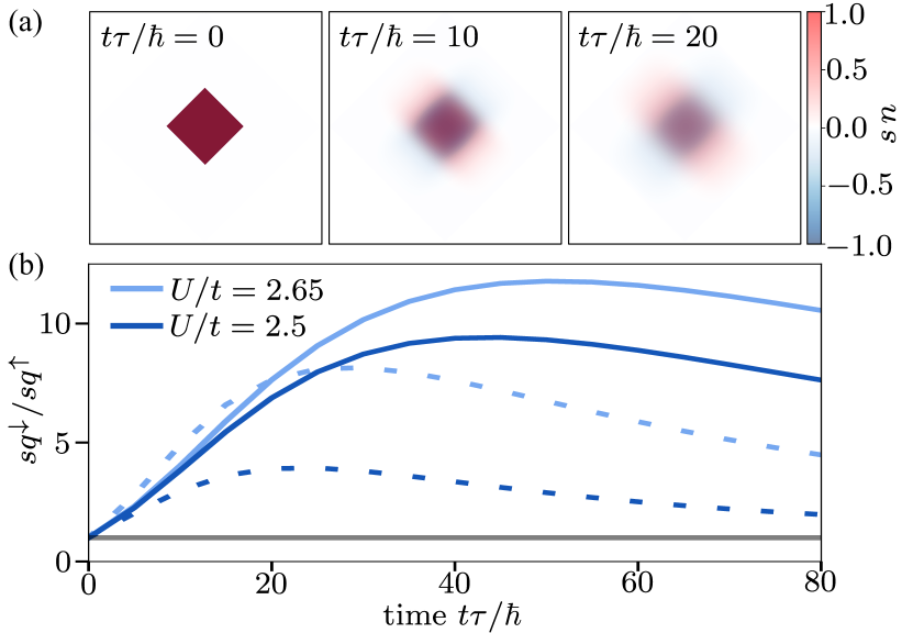
Figure 4: Anisotropic spin diffusion. (a) Trap-release dynamics of an altermagnetic state at finite temperature $T=0.2t$, trapped in a box potential in an optical lattice characterized by $V_{0}=4E_{r},V_{1}/V_{0}=2.2,\Delta=0.6$. The spin-resolved density propagates anisotropically in real space along the $\bm{a}_{1}$ and $\bm{a}_{2}$ directions. (b) We characterize the anisotropic expansion by the ratio of the geometric squeezing parameter ${sq}^{s}(\tau)$ of spin-down and spin-up atoms for two different values of the interaction $U$ and two different temperatures $T=0.15t$ (solid lines) and $T=0.2t$ (dashed lines). The grey line represents the isotropic expansion of a normal metallic state for which ${sq}^{s}(\tau)$ is always one.

We observe that the spin-up and spin-down atoms predominantly relax in different directions, related by a $\pi/2$ real-space rotation. The spin-up atoms have a larger contribution to $\sigma^{\uparrow}_{\tilde{y}\tilde{y}}$ than $\sigma^{\uparrow}_{\tilde{x}\tilde{x}}$ as can be also seen from the Fermi surface in the inset of Fig. 1 (b). Thus diffusion is stronger in the $\bm{a}_{2}$-direction than in $\bm{a}_{1}$ direction and vice versa for spin-down atoms. To quantify the anisotropy, we define a geometric squeezing parameter

$${sq}^{s}(\tau)=\frac{\int d^{2}\tilde{r}\,\tilde{x}^{2}\,n^{s}(\bm{\tilde{r}},t)}{\int d^{2}\tilde{r}\,\tilde{y}^{2}\,n^{s}(\bm{\tilde{r}},t)},$$ (8)

which measures the relative spread in $\tilde{x}$-direction compared to the $\tilde{y}$-direction. The relative squeezing of spin-down and spin-up $sq^{\downarrow}(\tau)/sq^{\uparrow}(\tau)$ initially increases strongly and then approaches one asympototically because the steady state is uniform in space; Fig. 4 (b).

When increasing the interaction strength $U$ the altermagnetic order parameter increases and by consequence also the spin-splitting energy, which leads to a larger squeezing parameter. For higher temperatures the anisotropy in the conductivity tensor is reduced as the spin splitting decreases. However, the initial growth of $sq^{\downarrow}(\tau)/sq^{\uparrow}(\tau)$ can be larger as overall the diffusion constant increases with temperature according to the Einstein relation.

Conclusions.—Altermagnetism represents a new type of collinear magnetism, distinct from ferromagnetism and antiferromagnetism, that is characterized by additional rotational symmetries between opposite spin sublattices. We have shown how such an altermagnetic state can be realized with fermionic ultracold atoms. As the underlying mechanism derives from the single-particle band structure, the state is robust and arises over a large parameter range. We discuss that the unconventional symmetry of the state can be detected experimentally in trap expansion experiments which exhibit anisotropic expansion for the different spin species.

Our work demonstrates the potential for ultracold atoms to provide a controllable platform for realizing and probing this new form of magnetism and for understanding the structure of fluctuations around the ordered states. For future work it would be interesting to characterize the anisotropic spin-susceptibilities of the altermagnetic state, which can be measured for example by Ramsey interferometry [35] or modulation spectroscopy [36]. Furthermore, the real-time dynamics of spin-wave excitations in the altermagnetic insulating state could unveil the unconventional symmetry of the state as well. An exciting direction is to explore the interplay of doped altermagnets and competing superconducting instabilities, which may offer a route to realize finite-momentum pairing or topological superconductivity.

Acknowledgements.— We acknowledge support from the Deutsche Forschungsgemeinschaft (DFG, German Research Foundation) under Germany’s Excellence Strategy–EXC–2111–390814868 and DFG Grants No. KN1254/1-2, KN1254/2-1, TRR 360 - 492547816, the European Research Council (ERC) under the European Union’s Horizon 2020 research and innovation programme (Grant Agreement No. 851161), as well as the Munich Quantum Valley, which is supported by the Bavarian state government with funds from the Hightech Agenda Bayern Plus. J.K. acknowledges support from the Imperial-TUM flagship partnership. V.L. acknowledges support from the Studienstiftung des deutschen Volkes. P.D. acknowledges support from the Working Internship in Science and Engineering (WISE) from the Deutscher Akademischer Austauschdienst (DAAD).

Data and Code availability.—Numerical data and simulation codes are available on Zenodo [37].

.1 Self-consistent Hartree-Fock Equations

We analyze the altermagnetic instabilities of our system within Hartree-Fock theory in which we decouple the interactions as $Un_{r\lambda\uparrow}n_{r\lambda\downarrow}\approx\hskip 5.69054ptUn_{r\lambda\uparrow}\left<n_{r\lambda\downarrow}\right>+U\left<n_{r\lambda\uparrow}\right>n_{r\lambda\downarrow}-U\left<n_{r\lambda\uparrow}\right>\left<n_{r\lambda\downarrow}\right>$, where $r$ is the index of a unit cell and $\lambda$ denotes the sub-lattice. Rewriting the interactions with the order paramter $\delta m$, defined in Eq. (2), we obtain

$$\begin{split}U\sum_{r,\lambda}n_{r\lambda\uparrow}&n_{r\lambda\downarrow}\approx\sum_{r,\lambda}-U\delta m(-1)^{\lambda}(n_{r\lambda\uparrow}-n_{r\lambda\downarrow})\\ &+U\frac{n}{2}(n_{r\lambda\uparrow}+n_{r\lambda\downarrow})-U\left(\frac{n^{2}}{4}-\delta m^{2}\right).\end{split}$$ (S1)

The last two terms in Eq. (S1) change only the chemical potential and add a constant energy shift, respectively, and thus do not modify our self-consistent solution. After Fourier transforming the total effective interaction and introducing the basis of $\Psi_{\bm{k}}^{\dagger}=(c_{{\bm{k}}A\uparrow}^{\dagger}c_{{\bm{k}}B\uparrow}^{\dagger}c_{{\bm{k}}A\downarrow}^{\dagger}c_{{\bm{k}}B\downarrow}^{\dagger})$, we obtain the mean-field Hamiltonian in Eq. (3).

The Hartree-Fock equations are solved by self-consistently determining the order parameter $\delta m$

$$\begin{split}\delta m&=\frac{1}{4N}\langle n_{A\uparrow}-n_{B\uparrow}-n_{A\downarrow}+n_{B\downarrow}\rangle_{\text{HF}}\\ \ &=\frac{1}{4N}\sum_{\bm{k},\alpha}\psi^{\dagger}_{\alpha}(\bm{k})\vbox{\hbox{$\begin{bmatrix}1&0&0&0\\ 0&-1&0&0\\ 0&0&-1&0\\ 0&0&0&1\\ \end{bmatrix}$}}\psi_{\alpha}(\bm{k})\cdot f(\epsilon_{\bm{k},\alpha}-\mu)\end{split}$$ (S2)

and the chemical potential $\mu$ which fixes the total density

$$\begin{split}n&=\frac{1}{2N}\langle n_{A\uparrow}+n_{B\uparrow}+n_{A\downarrow}+n_{B\downarrow}\rangle_{\text{HF}}\\ &=\frac{1}{2N}\sum_{\bm{k},\alpha}f(\epsilon_{\bm{k},\alpha}-\mu).\end{split}$$ (S3)

Here, $f(\epsilon_{\bm{k},\alpha}-\mu)$ is the Fermi distribution, $\epsilon_{\bm{k},\alpha}$, $\psi_{\alpha}(\bm{k})$ are the eigenvalues and eigenvectors of the matrix $H(\bm{k})=\text{diag}(H_{\uparrow}(\bm{k}),H_{\downarrow}(\bm{k}))$, $\alpha$ is the band index running from one to four, and $N$ is the total number of unit cells.

To self-consistently determine the order parameter $\delta m$ and the chemical potential $\mu$, we take a $200\times 200$ square grid of momentum points in the magnetic Brillouin zone. For each momentum we evaluate the matrix $H(\bm{k})=\text{diag}(H_{\uparrow}(\bm{k}),H_{\downarrow}(\bm{k}))$ and calculate the eigenvalues $\epsilon_{\alpha}(\bm{k})$ and eigenvectors $\psi_{\alpha}(\bm{k})$ of $H(\bm{k})$.

We solve the self-consistent equation by iteration. In each cycle of iteration we take an input value of $\delta m_{\text{in}}$ and calculate the resulting output $\delta m_{\text{out}}$ from Eq. (S2). In each iteration step we determine the chemical potential $\mu$ by fixing number of particles using Eq. (S3). For the next iteration loop we mix in 40% of the previous solution to improve convergence. We continue to run the iteration until the value of $\delta m$ converges to $|\delta m_{\text{out}}-\delta m_{\text{in}}|<10^{-6}$.

.2 Tight-Binding Parameters

By varying the optical lattice potential characterized by $V_{0},V_{1},\Delta$, the parameters of the tight-binding model can be adjusted. Here, we evaluate the tight-binding parameters $t$, $t^{\prime}$, and $\delta$ for fixed value of $V_{0}=4E_{r}$ as a function of $V_{1}$ and $\Delta$; see Fig. S1. We find for a large regime of optical lattice parameters, favorable tight-binding parameters for stabilizing altermagnetism.

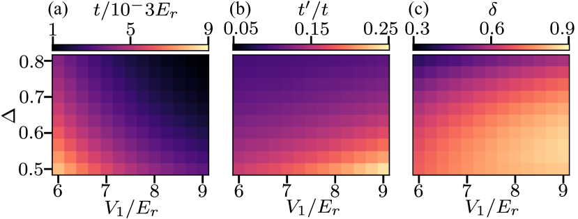
Figure S1: Tight-binding parameters. We compute the tight-binding parameters (a) nearest neighbor hopping $t/E_{r}$, (b) diagonal hopping $t^{\prime}/t$, and (c) diagonal hopping anisotropy $\delta$, as a function of the optical lattice parameters $V_{1}$ and $\Delta$ for fixed $V_{0}=4E_{r}$.

.3 Calculation of Conductivity Tensor

The conductivity tensor is a $2\times 2$ matrix for each spin

$$\begin{split}\sigma^{s}=\vbox{\hbox{$\begin{bmatrix}\sigma^{s}_{\tilde{x}\tilde{x}}&\sigma^{s}_{\tilde{x}\tilde{y}}\\ \sigma^{s}_{\tilde{y}\tilde{x}}&\sigma^{s}_{\tilde{y}\tilde{y}}\\ \end{bmatrix}$}}\end{split}$$ (S4)

We determine the matrix elements of the DC conductivity $\sigma_{\alpha\beta}^{s}(\omega\to 0)$ from the Kubo formula [32, 33, 34]

$$\sigma_{\alpha\alpha}^{s}(\omega\to 0) =\frac{\hbar}{4\pi V}\int_{-\infty}^{\infty}d\epsilon\frac{df}{d\epsilon}\text{Tr}\langle v_{\alpha}^{s}(G^{+}-G^{-})v_{\alpha}^{s}(G^{+}-G^{-})\rangle,$$ (S5)

where, $G^{\pm}(\epsilon)=[\epsilon-H\pm i\Gamma]^{-1}$ is the retarded/advanced Green’s function and $\bm{v}^{s}$ is the velocity defined as,

$$\begin{split}\bm{v}^{s}(\bm{k})=\frac{1}{\hbar}\nabla_{\bm{k}}H_{s}(\bm{k}),\end{split}$$ (S6)

where $H_{s}(\bm{k})$ is given in Eq. (3). The difference between the retarded and advanced Green’s functions is $G^{+}-G^{-}=-2i\pi\delta(\epsilon-H)$. For our numerical evaluation we replace the delta distribution by a Lorentian $\pi\delta(\epsilon-H)={\Gamma}/[{(\epsilon-H)^{2}+\Gamma^{2}}]$ with broadening $\Gamma=0.02$.

From diagonalizing the Hartree-Fock Hamiltonian $H(\bm{k})$ in Eq. (3) with self-consistently determined order parameter $\delta m$ and chemical potential $\mu$, we obtain the eigenvalues $\epsilon_{\alpha}(\bm{k})$ and eigenvectors $\psi_{\alpha}(\bm{k})$. We express the conductivity tensor in this basis as:

$$\begin{split}\sigma_{\alpha\alpha}^{s}&=\frac{\hbar}{4\pi V}\int_{-\infty}^{\infty}d\epsilon\frac{df}{d\epsilon}\sum_{m,n,\bm{k}}\langle\psi_{m}(\bm{k})|v_{\alpha}^{s}|\psi_{n}(\bm{k})\rangle(G^{+}-G^{-})(\epsilon_{n})\langle\psi_{n}(\textbf{k})|v_{i}|\psi_{m}(\bm{k})\rangle(G^{+}-G^{-})(\epsilon_{m})\\ &=-\frac{\hbar}{\pi V}\int_{-\infty}^{\infty}d\epsilon\frac{df}{d\epsilon}\sum_{m,n,\bm{k}}|\langle\psi_{m}(\bm{k})|v_{\alpha}^{s}|\psi_{n}(\bm{k})\rangle|^{2}\frac{\Gamma}{(\epsilon-\epsilon_{n})^{2}+\Gamma^{2}}\frac{\Gamma}{(\epsilon-\epsilon_{m})^{2}+\Gamma^{2}}.\end{split}$$ (S7)

We calculate Eq. (S7) numerically at finite temperature. At zero temperature, we further simplify the evaluation by using $\frac{df}{d\epsilon}=-\delta(\epsilon-\epsilon_{F})$.

References

- Ashcroft and Mermin [2022] N. W. Ashcroft and N. D. Mermin, Solid state physics (Cengage Learning, 2022).
- Auerbach [1998] A. Auerbach, Interacting electrons and quantum magnetism (Springer Science & Business Media, 1998).
- Wu et al. [2007] C. Wu, K. Sun, E. Fradkin, and S.-C. Zhang, Fermi liquid instabilities in the spin channel, Phys. Rev. B 75, 115103 (2007).
- Ahn et al. [2019] K.-H. Ahn, A. Hariki, K.-W. Lee, and J. Kuneš, Antiferromagnetism in as -wave pomeranchuk instability, Phys. Rev. B 99, 184432 (2019).
- Šmejkal et al. [2022a] L. Šmejkal, J. Sinova, and T. Jungwirth, Beyond conventional ferromagnetism and antiferromagnetism: A phase with nonrelativistic spin and crystal rotation symmetry, Phys. Rev. X 12, 031042 (2022a).
- Shao et al. [2021] D. Shao, S. Zhang, and M. e. a. Li, Spin-neutral currents for spintronics, Nat Commun 12, 7061 (2021).
- Šmejkal et al. [2022b] L. Šmejkal, J. Sinova, and T. Jungwirth, Emerging research landscape of altermagnetism, Phys. Rev. X 12, 040501 (2022b).
- Maier and Okamoto [2023] T. A. Maier and S. Okamoto, Weak-coupling theory of neutron scattering as a probe of altermagnetism, Phys. Rev. B 108, L100402 (2023).
- Krempaský et al. [2023] J. Krempaský, L. Šmejkal, S. W. D’Souza, M. Hajlaoui, G. Springholz, K. Uhlířová, F. Alarab, P. C. Constantinou, V. Strokov, D. Usanov, W. R. Pudelko, R. González-Hernández, A. B. Hellenes, Z. Jansa, H. Reichlová, Z. Šobáň, R. D. G. Betancourt, P. Wadley, J. Sinova, D. Kriegner, J. Minár, J. H. Dil, and T. Jungwirth, Altermagnetic lifting of kramers spin degeneracy, arXiv:2308.10681 (2023).
- Lee et al. [2023] S. Lee, S. Lee, S. Jung, J. Jung, D. Kim, Y. Lee, B. Seok, J. Kim, B. G. Park, L. Šmejkal, C.-J. Kang, and C. Kim, Broken kramers’ degeneracy in altermagnetic mnte, arXiv:2308.11180 (2023).
- Reimers et al. [2023] S. Reimers, L. Odenbreit, L. Smejkal, V. N. Strocov, P. Constantinou, A. B. Hellenes, R. J. Ubiergo, W. H. Campos, V. K. Bharadwaj, A. Chakraborty, T. Denneulin, W. Shi, R. E. Dunin-Borkowski, S. Das, M. Kläui, J. Sinova, and M. Jourdan, Direct observation of altermagnetic band splitting in crsb thin films, arXiv:2310.17280 (2023).
- Feng et al. [2022] Z. Feng, X. Zhou, L. Šmejkal, L. Wu, Z. Zhu, H. Guo, R. González-Hernández, X. Wang, H. Yan, P. Qin, X. Zhang, H. Wu, H. Chen, Z. Meng, L. Liu, Z. Xia, J. Sinova, T. Jungwirth, and Z. Liu, An anomalous hall effect in altermagnetic ruthenium dioxide, Nature Electronics 5, 735 (2022).
- Mazin [2022] I. Mazin (The PRX Editors), Editorial: Altermagnetism—a new punch line of fundamental magnetism, Phys. Rev. X 12, 040002 (2022).
- Bloch et al. [2008] I. Bloch, J. Dalibard, and W. Zwerger, Many-body physics with ultracold gases, Rev. Mod. Phys. 80, 885 (2008).
- Jördens et al. [2008] R. Jördens, N. Strohmaier, K. Günter, H. Moritz, and T. Esslinger, A mott insulator of fermionic atoms in an optical lattice, Nature 455, 204–207 (2008).
- Schneider et al. [2008] U. Schneider, L. Hackermüller, S. Will, T. Best, I. Bloch, T. A. Costi, R. W. Helmes, D. Rasch, and A. Rosch, Metallic and insulating phases of repulsively interacting fermions in a 3d optical lattice, Science 322, 1520–1525 (2008).
- Hart et al. [2015] R. A. Hart, P. M. Duarte, T.-L. Yang, X. Liu, T. Paiva, E. Khatami, R. T. Scalettar, N. Trivedi, D. A. Huse, and R. G. Hulet, Observation of antiferromagnetic correlations in the hubbard model with ultracold atoms, Nature 519, 211–214 (2015).
- Mazurenko et al. [2017] A. Mazurenko, C. S. Chiu, G. Ji, M. F. Parsons, M. Kanász-Nagy, R. Schmidt, F. Grusdt, E. Demler, D. Greif, and M. Greiner, A cold-atom fermi–hubbard antiferromagnet, Nature 545, 462–466 (2017).
- Chiu et al. [2019] C. S. Chiu, G. Ji, A. Bohrdt, M. Xu, M. Knap, E. Demler, F. Grusdt, M. Greiner, and D. Greif, String patterns in the doped hubbard model, Science 365, 251–256 (2019).
- Bohrdt et al. [2019] A. Bohrdt, C. S. Chiu, G. Ji, M. Xu, D. Greif, M. Greiner, E. Demler, F. Grusdt, and M. Knap, Classifying snapshots of the doped hubbard model with machine learning, Nature Physics 15, 921–924 (2019).
- Koepsell et al. [2021] J. Koepsell, D. Bourgund, P. Sompet, S. Hirthe, A. Bohrdt, Y. Wang, F. Grusdt, E. Demler, G. Salomon, C. Gross, and I. Bloch, Microscopic evolution of doped mott insulators from polaronic metal to fermi liquid, Science 374, 82–86 (2021).
- Bohrdt et al. [2021] A. Bohrdt, L. Homeier, C. Reinmoser, E. Demler, and F. Grusdt, Exploration of doped quantum magnets with ultracold atoms, Annals of Physics 435, 168651 (2021).
- Mongkolkiattichai et al. [2023] J. Mongkolkiattichai, L. Liu, D. Garwood, J. Yang, and P. Schauss, Quantum gas microscopy of fermionic triangular-lattice mott insulators, Phys. Rev. A 108, L061301 (2023).
- Xu et al. [2023] M. Xu, L. H. Kendrick, A. Kale, Y. Gang, G. Ji, R. T. Scalettar, M. Lebrat, and M. Greiner, Frustration- and doping-induced magnetism in a fermi–hubbard simulator, Nature 620, 971–976 (2023).
- Lebrat et al. [2023] M. Lebrat, M. Xu, L. H. Kendrick, A. Kale, Y. Gang, P. Seetharaman, I. Morera, E. Khatami, E. Demler, and M. Greiner, Observation of Nagaoka Polarons in a Fermi-Hubbard Quantum Simulator, arXiv:2308.12269 (2023).
- Prichard et al. [2023] M. L. Prichard, B. M. Spar, I. Morera, E. Demler, Z. Z. Yan, and W. S. Bakr, Directly imaging spin polarons in a kinetically frustrated Hubbard system, arXiv:2308.12951 (2023).
- [27] see supplementary material.
- Chin et al. [2010] C. Chin, R. Grimm, P. Julienne, and E. Tiesinga, Feshbach resonances in ultracold gases, Reviews of Modern Physics 82, 1225–1286 (2010).
- Bissbort [2013] U. Bissbort, Dynamical effects and disorder in ultracold bosonic matter, doctoralthesis, Universitätsbibliothek Johann Christian Senckenberg (2013).
- Šmejkal et al. [2020] L. Šmejkal, R. González-Hernández, T. Jungwirth, and J. Sinova, Crystal time-reversal symmetry breaking and spontaneous hall effect in collinear antiferromagnets, Science Advances 6, eaaz8809 (2020).
- González-Hernández et al. [2021] R. González-Hernández, L. Šmejkal, K. Výborný, Y. Yahagi, J. Sinova, T. c. v. Jungwirth, and J. Železný, Efficient electrical spin splitter based on nonrelativistic collinear antiferromagnetism, Phys. Rev. Lett. 126, 127701 (2021).
- Kubo [1957] R. Kubo, Statistical-mechanical theory of irreversible processes. i. general theory and simple applications to magnetic and conduction problems, Journal of the Physical Society of Japan 12, 570 (1957).
- Crépieux and Bruno [2001] A. Crépieux and P. Bruno, Theory of the anomalous hall effect from the kubo formula and the dirac equation, Phys. Rev. B 64, 014416 (2001).
- Freimuth et al. [2014] F. Freimuth, S. Blügel, and Y. Mokrousov, Spin-orbit torques in co/pt(111) and mn/w(001) magnetic bilayers from first principles, Phys. Rev. B 90, 174423 (2014).
- Knap et al. [2013] M. Knap, A. Kantian, T. Giamarchi, I. Bloch, M. D. Lukin, and E. Demler, Probing real-space and time-resolved correlation functions with many-body ramsey interferometry, Phys. Rev. Lett. 111, 147205 (2013).
- Bohrdt et al. [2018] A. Bohrdt, D. Greif, E. Demler, M. Knap, and F. Grusdt, Angle-resolved photoemission spectroscopy with quantum gas microscopes, Phys. Rev. B 97, 125117 (2018).
- [37] All data and simulation codes are available upon reasonable request at 10.5281/zenodo.10391823.
Supplemental Material: