Relations between Markovian and non-Markovian correlations in multi-time quantum processes

Abstract

In the dynamics of open quantum systems, information may propagate in time through either the system or the environment, giving rise to Markovian and non-Markovian temporal correlations, respectively. However, despite their notable coexistence in most physical situations, it is not yet clear how these two quantities may limit the existence of one another. Here, we address this issue by deriving several inequalities relating the temporal correlations of general multi-time quantum processes. The dynamics are described by process tensors and the correlations are quantified by the mutual information between subsystems of their Choi states. First, we prove a set of upper bounds to the non-Markovianity of a process given the degree of Markovianity in each of its steps. This immediately implies a non-trivial maximum value for the non-Markovianity of any process, independently of its Markovianity. Finally, we obtain how the non-Markovianity limits the amount of total temporal correlations that could be present in a given process. These results show that, although any multi-time process must pay a price in total correlations to have a given amount of non-Markovianity, this price vanishes exponentially with the number of steps of the process, while the maximum non-Markovianity grows only linearly. This implies that even a highly non-Markovian process might be arbitrarily close to having maximum total correlations if it has a sufficiently large number of steps.

1 Introduction

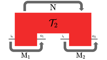
Figure 1: Markovian and non-Markovian correlations in a two-step quantum process. While $\mathrm{M}_{j}$ quantifies how much information is transmitted through the system in the $j$-th step, $\mathrm{N}$ quantifies how much information is transmitted through the environment from the first step to the second one. In this two-step setting, we show that $\mathrm{N}\leq 2\quantity(2\log d-\mathrm{M}_{1})$ and $\mathrm{N}\leq 2\log d-\mathrm{M}_{2}$. The generalization of this result to the $n$-step scenario implies that the maximum non-Markovianity of an $n$-step process tensor is $2(n-1)\log d$, and not $2n\log d$ as it could seem at first, and also that the total correlations $\mathrm{I}$ of the process are upper bounded by $2n\log d-\mathrm{N}/(2^{n}-2)$, meaning that a process can only approach the maximum amount $2n\log d$ of total correlations if it has low non-Markovianity or a large number of steps.

Understanding how information flows in quantum processes is a central task for developing quantum technologies and for better comprehending fundamental aspects of quantum theory. As any quantum system of interest inevitably interacts with an uncontrolled environment [1, 2], crucial information stored on the system may get lost along the dynamics [3, 4], which constitutes the main challenge for experimental implementation of quantum information processing protocols [5].

Sometimes, however, this information returns. Such information backflow is what characterizes non-Markovian quantum processes [6, 7, 8, 9], whose dynamics are best described within the process tensor framework [10]. Unlike traditional approaches, that typically employ quantum channels mapping an initial state to an evolved one [1, 2, 3, 4], process tensors are generalizations of joint probabilities to the quantum realm [11], which allows for a consistent definition of quantum Markovianity [12] and a proper treatment of memory effects [13, 14, 15, 16, 17, 18, 19, 20, 21, 22, 23, 24].

This way, several fields of quantum theory that had so far only been explored for Markovian dynamics are now being expanded to non-Markovian settings, which brings them closer to practical applications of the theory since, like in classical stochastic processes [25, 26], non-Markovianity is the rule in nature, not the exception. Examples of this may be found in the fields of quantum simulation [27, 28, 29, 30, 31, 32, 33, 34], randomized benchmarking [35, 36, 37], quantum process tomography [38, 39, 40, 41, 42, 43, 44], quantum thermodynamics [45, 46, 47, 48, 49, 50], among others [51, 52, 53].

The main feature that allows for process tensors to best describe non-Markovian dynamics is their genuine multi-time structure, which may be equivalently characterized by means of quantum combs [54] or quantum networks [55]. Similarly, one could also consider treating such correlations with slightly more general objects called process matrices, which are used in the context of quantum causal modeling as they can also describe processes with indefinite causal order [56, 57, 58, 59, 60, 61, 62]. This way, we could say that a process tensor is a time-ordered process matrix.

Importantly, it has been shown that one can construct resource theories of quantum process, which take process tensors as objects and superprocesses as transformations [63]. This is extremely useful, as it allows one to take relevant concepts, techniques and even results from other resource theories and adapt them to the context of quantum processes. For example, Ref. [64] proved that non-Markovianity and time resolution of a process could be consumed as resources to reduce noise in a given process. This is done by means of an optimized dynamical decoupling protocol that takes the memory effects of the process into account.

As it is usually the case for resource theories [65], monotones play a central role in the resource theory of quantum processes. Ref. [64] defines three important information quantifiers for general multi-time processes: Markovian correlations, non-Markovian correlations and total correlations, and shows them to be monotonic under the free operations of the theory. Here, we take one step further in this direction and seek relevant properties of these quantifiers. We use the notion of information exchange between system and environment and the time-ordering of the process to prove several inequalities relating the multi-time correlations of any given quantum process. A summary of our results is shown in Fig. 1.

This paper is structured as follows. In Sec. 2 we show how the approach we use to quantify temporal correlations applies for single-step processes, as described by quantum channels. In Sec. 3 we present the two-step scenario, which is the simplest one where non-Markovianity may take place, and discuss from an informational standpoint why Markovian and non-Markovian correlations should limit one another, proving some insightful bounds for this simple case. In Sec. 4 the previous analyses are put on firm mathematical grounds and the results are generalized to the $n$-step scenario. The discussions are then concluded in Sec. 5.

2 Temporal correlations in single-step quantum processes

Quantum channels are the simplest descriptors of open quantum systems dynamics. They are linear, completely positive and trace-preserving (CPTP) maps, which take an initial state of the system as input and provide as output the corresponding final state after a single interaction with the environment [3, 4]. An example of quantum channel which will be present throughout this text is the depolarizing channel $\mathcal{E}_{p}:\mathcal{B}(\mathcal{H}_{\mathrm{in}})\to\mathcal{B}(\mathcal{H}_{\mathrm{out}})$, whose action is defined as

$$\mathcal{E}_{p}(\rho)=p\tilde{\mathbb{I}}+(1-p)\rho,$$ (1)

where $\tilde{\mathbb{I}}=\mathbb{I}/d$ is the maximally mixed state, $d$ is the dimension of the system and $p\in[0,1]$ is a parameter of the channel. For $p=0$ we have an identity channel $\mathcal{E}_{0}(\rho)=\rho$, implying that in this case all the information about the initial state is preserved in the final state, such that the input and output are maximally correlated. On the other hand, for $p=1$ we have the completely depolarizing channel $\mathcal{E}_{1}(\rho)=\tilde{\mathbb{I}}$, which means that all the information about the initial state is lost during the process, i.e., input and output are totally uncorrelated.

The amount of information that is preserved or lost in a quantum channel may be quantified in several ways. Here, we adopt an approach that has been shown to be well suited for multi-time processes, which consists in first mapping the temporal correlations of the process into spatial correlations of a corresponding state and then applying distance-based measures to quantify them [12, 64].

The first step is achieved using the Choi-Jamiolkowski isomorphism, in which a channel $\mathcal{E}:\mathcal{B}(\mathcal{H}_{\mathrm{in}})\to\mathcal{B}(\mathcal{H}_{\mathrm{out}})$ is mapped to a state $\Upsilon^{\mathcal{E}}\in\mathcal{B}(\mathcal{H}_{\mathrm{in}}\otimes\mathcal{H}_{\mathrm{out}})$ by means of

$$\Upsilon^{\mathcal{E}}\coloneqq\quantity(\mathcal{I}_{\mathrm{in}}\otimes\mathcal{E})\Phi,$$ (2)

where

$$\Phi=\frac{1}{d}\sum_{i,j=1}^{d}\ket{i}\bra{j}_{\mathrm{in}}\otimes\ket{i}\bra{j}_{\mathrm{in}}$$ (3)

is a normalized maximally entangled state in $\mathcal{B}(\mathcal{H}_{\mathrm{in}}\otimes\mathcal{H}_{\mathrm{in}})$ and $\mathcal{I}_{\mathrm{in}}$ is the identity channel in $\mathcal{B}(\mathcal{H}_{\mathrm{in}})$. The trace preservation of $\mathcal{E}$, which corresponds to its deterministic implementation, implies the trace condition

$$\tr_{\mathrm{out}}\quantity[\Upsilon^{\mathcal{E}}]=\tilde{\mathbb{I}}_{\mathrm{in}}.$$ (4)

In turn, any quantum state $\Upsilon\in\mathcal{B}(\mathcal{H}_{\mathrm{in}}\otimes\mathcal{H}_{\mathrm{out}})$ satisfying the above condition may be associated to a quantum channel $\mathcal{E}^{\Upsilon}:\mathcal{B}(\mathcal{H}_{\mathrm{in}})\to\mathcal{B}(\mathcal{H}_{\mathrm{out}})$ by

$$\mathcal{E}^{\Upsilon}(\rho_{\mathrm{in}})=d\tr_{\mathrm{in}}\quantity[\quantity(\rho_{\mathrm{in}}\otimes\tilde{\mathbb{I}}_{\mathrm{out}})\Upsilon^{T_{\mathrm{in}}}],$$ (5)

where $T_{\mathrm{in}}$ represents the partial transpose in the $\ket{i}$ basis of $\mathcal{H}_{\mathrm{in}}$.

Since the Choi state $\Upsilon^{\mathcal{E}}$ contains all the information about the quantum channel $\mathcal{E}$, the temporal correlations of the channel are mapped into spatial correlations between the subspaces $\mathcal{H}_{\mathrm{in}}$ and $\mathcal{H}_{\mathrm{out}}$ of $\Upsilon^{\mathcal{E}}$. For example,

$$\Upsilon^{\mathcal{E}}=\tilde{\mathbb{I}}_{\mathrm{in}}\otimes\sigma_{\mathrm{out}}\iff\mathcal{E}(\rho_{\mathrm{in}})=\sigma_{\mathrm{out}}\leavevmode\nobreak\ \leavevmode\nobreak\ \leavevmode\nobreak\ \forall\rho_{\mathrm{in}},$$ (6)

that is, the Choi state is a product state iff the channel has a fixed output (i.e., having no spatial correlations is equivalent to having no temporal correlations). On the other hand, the Choi state is maximally entangled iff the channel is unitary, and it is separable iff the channel is entanglement-breaking [66].

Now, to quantify the spatial correlations of Choi states we apply the mutual information between subspaces, which is equivalent to the relative entropy between the state and the closest uncorrelated state [4, 64],

$$\mathrm{I}(\mathrm{A}:\mathrm{B})_{\rho_{\mathrm{AB}}} \coloneqq S_{\mathrm{A}}+S_{\mathrm{B}}-S_{\mathrm{AB}}$$ (7)

$$=S(\rho_{\mathrm{AB}}||\rho_{\mathrm{A}}\otimes\rho_{\mathrm{B}}),$$ (8)

where $S_{\mathrm{A}}=-\tr[\rho_{\mathrm{A}}\log\rho_{\mathrm{A}}]$ is the von Neumann entropy of $\rho_{\mathrm{A}}=\tr_{\mathrm{B}}\quantity[\rho_{\mathrm{AB}}]$ and $S(\rho||\sigma)=\tr[\rho\quantity(\log\rho-\log\sigma)]$ is the relative entropy quasi-distance between the states $\rho$ and $\sigma$. This way, we can define the input-output correlation of the channel $\mathcal{E}$ by

$$\mathrm{M}(\mathcal{E}) \coloneqq\mathrm{I}(\mathrm{in}:\mathrm{out})_{\Upsilon^{\mathcal{E}}}$$ (9)

$$=S_{\mathrm{in}}+S_{\mathrm{out}}-S_{\mathrm{in}\leavevmode\nobreak\ \mathrm{out}}.$$ (10)

To illustrate how $\mathrm{M}$ quantifies the amount of information preserved by a given quantum channel, in Fig. 2 we plot $\mathrm{M}(\mathcal{E}_{p})$ as a function of $p$ for the depolarizing channel.

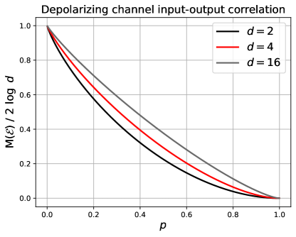
Figure 2: Input-output correlation of the depolarizing channel for different dimensions of the system. $\mathrm{M}(\mathcal{E}_{p})$ is a monotonic function of $p$ for any $d$. In general, the quantity $\mathrm{M}(\mathcal{E})$ ranges from $0$, for fixed output channels, to $2\log d$, for unitary channels.

To better understand the informational interplay between system and environment, consider the Stinespring dilation theorem [67, 3, 4], according to which the action of any given channel $\mathcal{E}$ may be represented as

$$\mathcal{E}(\rho)=\tr_{\mathrm{E}}\quantity[U(\rho\otimes\sigma_{\mathrm{E}})U^{\dagger}],$$ (11)

for some initial state $\sigma_{\mathrm{E}}\in\mathcal{B}(\mathcal{H}_{\mathrm{E}})$ of the environment and some global unitary $U:\mathcal{B}(\mathcal{H}_{\mathrm{in}}\otimes\mathcal{H}_{\mathrm{E}})\to\mathcal{B}(\mathcal{H}_{\mathrm{out}}\otimes\mathcal{H}_{\mathrm{E}})$. Fig. 3 shows a possible dilation for the depolarizing channel.

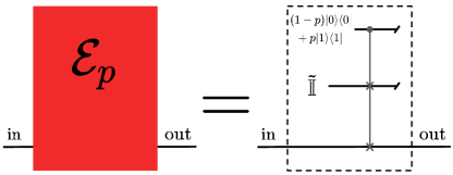
Figure 3: Example of a Stinespring dilation for the depolarizing channel of Eq. (1). The global unitary is a controlled-swap (Fredkin) gate, the initial state of the control space of the environment is $(1-p)\ket{0}\bra{0}+p\ket{1}\bra{1}$ and the initial state of the target space of the environment is $\tilde{\mathbb{I}}$. This way, the input state $\rho$ of the system is swapped with $\tilde{\mathbb{I}}$ conditioned on the state of the control space. Tracing out the environment yields a depolarizing reduced dynamics for the system.

Now, consider a purification $\Psi_{\mathrm{ER}}=\ket{\psi}\bra{\psi}\in\mathcal{B}(\mathcal{H}_{\mathrm{E}}\otimes\mathcal{H}_{\mathrm{R}})$ of $\sigma_{\mathrm{E}}$ to a system $\mathrm{R}$, that is,

$$\tr_{\scaleto{\mathrm{R}}{5pt}}\quantity[\Psi_{\mathrm{ER}}]=\sigma_{\mathrm{E}},$$ (12)

and define a global pure state $\eta\in\mathcal{B}(\mathcal{H}_{\mathrm{in}}\otimes\mathcal{H}_{\mathrm{out}}\mathcal{H}_{\mathrm{E}}\otimes\mathcal{H}_{\mathrm{R}})$ after the unitary interaction

$$\eta\coloneqq\quantity(\mathcal{I}_{\mathrm{in}}\otimes\mathcal{U}^{\mathrm{in},\mathrm{E}}_{\mathrm{out},\mathrm{E}}\otimes\mathcal{I}_{\mathrm{R}})\quantity(\Phi\otimes\Psi_{\mathrm{ER}}).$$ (13)

Comparing this definition to Eqs. (9) and (11), it is immediate that

$$\mathrm{I}(\mathrm{in}:\mathrm{out})_{\eta}=\mathrm{M}.$$ (14)

By defining the complement of $\mathrm{M}$ as

$$\overline{\mathrm{M}}\coloneqq 2\log d-\mathrm{M},$$ (15)

it follows that

$$\mathrm{I}(\mathrm{in}:\mathrm{E}\mathrm{R})_{\eta} =S_{\mathrm{in}}+S_{\mathrm{E}\mathrm{R}}-S_{\mathrm{in}\leavevmode\nobreak\ \mathrm{E}\mathrm{R}}$$ (16)

$$=S_{\mathrm{in}}+S_{\mathrm{in}\leavevmode\nobreak\ \mathrm{out}}-S_{\mathrm{out}}$$ (17)

$$=2S_{\mathrm{in}}-(S_{\mathrm{in}}+S_{\mathrm{out}}-S_{\mathrm{in}\leavevmode\nobreak\ \mathrm{out}})$$ (18)

$$=2\log d-\mathrm{M}$$ (19)

$$=\overline{\mathrm{M}},$$ (20)

where we used $S_{\mathrm{E}\mathrm{R}}=S_{\mathrm{in}\leavevmode\nobreak\ \mathrm{out}}$ and $S_{\mathrm{in}\leavevmode\nobreak\ \mathrm{E}\mathrm{R}}=S_{\mathrm{out}}$ since bipartitions of pure states share the same entropy [3, 4], and also $S_{\mathrm{in}}=\log d$ as from Eq. (4) we know $\tr_{\scaleto{\mathrm{out}\mathrm{E}\mathrm{R}}{5pt}}\quantity[\eta]$ is maximally mixed. Eq. (20) shows that, while $\mathrm{M}$ is the information about the initial state of the system that is kept in its the final state, $\overline{\mathrm{M}}$ is exactly the part of this information that is lost to the environment. In turn, the system might also get some information about the initial state of the environment. Since this information is useless for us, it is simply treated as noise. However, this will not always be the case in multi-time processes, as at any time step that is not the first one the environment may be carrying information about past states of the system.

Importantly, we can show that for the system to get this information from the environment, it must also give some of its own. To see this, notice that

$$\mathrm{I}(\mathrm{in}\leavevmode\nobreak\ \mathrm{out}:\mathrm{R})_{\eta} =S_{\mathrm{in}\leavevmode\nobreak\ \mathrm{out}}+S_{\mathrm{R}}-S_{\mathrm{in}\leavevmode\nobreak\ \mathrm{out}\leavevmode\nobreak\ \mathrm{R}}$$ (21)

$$\leq 2S_{\mathrm{in}\leavevmode\nobreak\ \mathrm{out}}$$ (22)

$$=2(S_{\mathrm{in}}+S_{\mathrm{out}}-\mathrm{M})$$ (23)

$$\leq 2(2\log d-\mathrm{M})$$ (24)

$$=2\overline{\mathrm{M}},$$ (25)

where the relation $S_{\mathrm{R}}-S_{\mathrm{in}\leavevmode\nobreak\ \mathrm{out}\leavevmode\nobreak\ \mathrm{R}}\leq S_{\mathrm{in}\leavevmode\nobreak\ \mathrm{out}}$ is a consequence of Araki-Lieb triangle inequality [68]

$$|S_{\mathrm{A}}-S_{\mathrm{B}}|\leq S_{\mathrm{AB}},$$ (26)

and we also used $S_{\mathrm{in}}+S_{\mathrm{out}}\leq 2\log d$. Eq. (25) means the amount of information the system might receive about the initial state of the environment is upper bounded by twice the amount of information the environment receives about the initial state of the system. This intuition on information exchange between system and environment lies at the heart of our relations between temporal correlations in multi-time processes.

3 Temporal correlations in two-step quantum processes

Besides the single-step processes described by quantum channels, one could also consider a two-step scenario, as depicted in Fig. 4. Notice that in this case the action of the environment on the system will not in general be described by a quantum channel in each step, as the global state before the second step might not be a product one and, even if it is, the state of the environment might be conditioned on the input state at time $t_{0}$. Thus, the most general descriptor of the action of the environment in the two-step scenario will be a mapping $\mathcal{T}_{2}$ taking both the initial state and the control operation to the final state,

$$\mathcal{T}_{2}\quantity[\rho\otimes\mathcal{M}_{1}]=\rho^{\prime}.$$ (27)

To preserve the physical properties of the process, this mapping must be multi-linear, completely positive, trace-preserving and time-ordered. A mapping $\mathcal{T}_{2}:\mathcal{B}(\mathcal{H}_{\mathrm{A}})\otimes\mathcal{B}^{2}(\mathcal{H}_{\mathrm{B}},\mathcal{H}_{\mathrm{C}})\to\mathcal{B}(\mathcal{H}_{\mathrm{D}})$ satisfying these conditions is what we call a two-step process tensor [10].

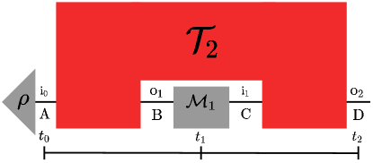
Figure 4: The two-step scenario. Initially, an experimenter prepares the system in a state $\rho$ as input at time $t_{0}$. Then, the system interacts with the environment in a first step, resulting in a new output state at time $t_{1}$. Next, the experimenter performs a control operation on the system alone, as described by a quantum channel $\mathcal{M}_{1}:\mathcal{B}(\mathcal{H}_{\mathrm{o}_{1}})\to\mathcal{B}(\mathcal{H}_{\mathrm{i}_{1}})$. Finally, still at time $t_{1}$, the system interacts in a second step with the same environment as before, yielding a final state at time $t_{2}$. The Hilbert space labels above the lines in the figure describe if the corresponding state at a given time is the input or the output of an interaction with the environment, such that $\mathrm{o}_{1}$ is the output space at time $t_{1}$, for example. As a consequence of this convention, the experimenter operations will be mappings from output spaces to input spaces at fixed times. To simplify the notation, for the remainder of this section we adopt the Hilbert space labeling shown below the lines in the figure, that is, we use $\{\mathrm{A},\mathrm{B},\mathrm{C},\mathrm{D}\}$ instead of $\{\mathrm{i}_{0},\mathrm{o}_{1},\mathrm{i}_{1},\mathrm{o}_{2}\}$. This more descriptive labeling will be recovered in the discussion of the multi-time scenario in Section 4.

Alternatively, $\mathcal{T}_{2}$ might be seen as a mapping from two input spaces to two output spaces, $\mathcal{T}_{2}:\mathcal{B}(\mathcal{H}_{\mathrm{A}}\otimes\mathcal{H}_{\mathrm{B}})\to\mathcal{B}(\mathcal{H}_{\mathrm{C}}\otimes\mathcal{H}_{\mathrm{D}})$. This way, we define the Choi state $\Upsilon^{\mathcal{T}_{2}}\in\mathcal{B}(\mathcal{H}_{\mathrm{A}}\otimes\mathcal{H}_{\mathrm{B}}\otimes\mathcal{H}_{\mathrm{C}}\otimes\mathcal{H}_{\mathrm{D}})$ of the process tensor $\mathcal{T}_{2}$ by

$$\Upsilon^{\mathcal{T}_{2}}\coloneqq\quantity(\mathcal{I}_{\mathrm{A}}\otimes\mathcal{I}_{\mathrm{C}}\otimes\mathcal{T}_{2})\quantity(\Phi_{\mathrm{A}\mathrm{A}}\otimes\Phi_{\mathrm{C}\mathrm{C}}),$$ (28)

as shown in Fig. 5. In terms of its Choi state, the trace-preservation and time-ordering properties of the two-step process tensor $\mathcal{T}_{2}$ are given by

$$\tr_{\scaleto{\mathrm{D}}{5pt}}\quantity[\Upsilon^{\mathcal{T}_{2}}]=\tr_{\scaleto{\mathrm{C}\mathrm{D}}{5pt}}\quantity[\Upsilon^{\mathcal{T}_{2}}]\otimes\tilde{\mathbb{I}}_{\scaleto{\mathrm{C}}{5pt}},$$ (29)

$$\tr_{\scaleto{\mathrm{B}\mathrm{C}\mathrm{D}}{5pt}}\quantity[\Upsilon^{\mathcal{T}_{2}}]=\tilde{\mathbb{I}}_{\scaleto{\mathrm{A}}{5pt}}.$$ (30)

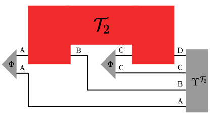
Figure 5: Circuit generating the Choi state of a given process tensor $\mathcal{T}_{2}$. At each time step we prepare a maximally entangled state $\Phi$ and store half of the state while letting the other half interact with the environment. The state of the system after each interaction is then also stored. The global quadripartite state stored in the end is the Choi state of the process tensor describing this two-step process.

Like in the single-step scenario, the temporal correlations of the two-step process are mapped into spatial correlations of its Choi state, with the additional feature that in this case there is more than just an input-output correlation. We follow Ref. [64] and define the total correlations of the process $\mathcal{T}_{2}$

$$\mathrm{I}(\mathcal{T}_{2})\coloneqq \leavevmode\nobreak\ \mathrm{I}(\mathrm{A}:\mathrm{B}:\mathrm{C}:\mathrm{D})_{\Upsilon^{\mathcal{T}_{2}}}$$ (31)

$$= \leavevmode\nobreak\ S_{\mathrm{A}}+S_{\mathrm{B}}+S_{\mathrm{C}}+S_{\mathrm{D}}-S_{\mathrm{A}\mathrm{B}\mathrm{C}\mathrm{D}},$$ (32)

the Markovian correlations in the first step

$$\mathrm{M}_{1}(\mathcal{T}_{2})\coloneqq \leavevmode\nobreak\ \mathrm{I}(\mathrm{A}:\mathrm{B})_{\Upsilon^{\mathcal{T}_{2}}}$$ (33)

$$= \leavevmode\nobreak\ S_{\mathrm{A}}+S_{\mathrm{B}}-S_{\mathrm{A}\mathrm{B}},$$ (34)

the Markovian correlations in the second step

$$\mathrm{M}_{2}(\mathcal{T}_{2})\coloneqq \leavevmode\nobreak\ \mathrm{I}(\mathrm{C}:\mathrm{D})_{\Upsilon^{\mathcal{T}_{2}}}$$ (35)

$$= \leavevmode\nobreak\ S_{\mathrm{C}}+S_{\mathrm{D}}-S_{\mathrm{C}\mathrm{D}},$$ (36)

the total Markovian correlations

$$\mathrm{M}\coloneqq \leavevmode\nobreak\ \mathrm{M}_{1}+\mathrm{M}_{2},$$ (37)

and the non-Markovian correlations

$$\mathrm{N}(\mathcal{T}_{2})\coloneqq \leavevmode\nobreak\ \mathrm{I}(\mathrm{A}\mathrm{B}:\mathrm{C}\mathrm{D})_{\Upsilon^{\mathcal{T}_{2}}}$$ (38)

$$= \leavevmode\nobreak\ S_{\mathrm{A}\mathrm{B}}+S_{\mathrm{C}\mathrm{D}}-S_{\mathrm{A}\mathrm{B}\mathrm{C}\mathrm{D}},$$ (39)

immediately implying the additive property

$$\mathrm{I} =\mathrm{M}+\mathrm{N}$$ (40)

$$=\mathrm{M}_{1}+\mathrm{M}_{2}+\mathrm{N},$$ (41)

for any two-step process $\mathcal{T}_{2}$.

Notice that $\mathrm{M}_{1}$ is the input-output correlation, as defined in Eq. (9), for the channel describing the first step of the process $\mathcal{T}_{2}$, which is associated to the Choi state $\tr_{\scaleto{\mathrm{C}\mathrm{D}}{5pt}}[\Upsilon^{\mathcal{T}_{2}}]$. Moreover, we could obtain a channel in the second step by averaging over all possible inputs in the first step of $\mathcal{T}_{2}$. Such channel, whose Choi state is $\tr_{\scaleto{\mathrm{A}\mathrm{B}}{5pt}}[\Upsilon^{\mathcal{T}_{2}}]$, would have an input-output correlation equal to $\mathrm{M}_{2}$. Finally, although we could see that $\mathrm{N}$ is a measure of correlations between the two steps, it might not be fully clear why it should be associated to the non-Markovianity of the process. To clarify this, we recall the operational Markov condition given in Ref. [12], according to which a process is Markovian if its Choi state is of the form

$$\Upsilon_{\mathrm{A}\mathrm{B}\mathrm{C}\mathrm{D}}=\Upsilon_{\mathrm{A}\mathrm{B}}\otimes\Upsilon_{\mathrm{C}\mathrm{D}},$$ (42)

implying the distance between any given Choi state and the closest Markov Choi state will measure the degree of non-Markovianity of the process. This way, since the $\mathrm{N}$ we defined in Eq. (38) is the relative entropy between $\Upsilon^{\mathcal{T}_{2}}$ and the closest Markov Choi state, it will be a non-Markovianity quantifier following the recipe of Ref. [12]. A schematic representation of the Markovian and non-Markovian correlations in a two-step quantum process is shown in Fig. 1. As an example of how these correlations may coexist in a physical situation, we consider the two-step non-Markovian depolarizing dynamics shown in Fig. 6. In Fig. 7 we see how they vary as a function of the parameter $p$.

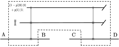
Figure 6: Two-step non-Markovian depolarizing dynamics. The first step of this dynamics is equal to the single-step process described in Fig. 3, where depending on the state of the control system the input state is exchanged with a maximally mixed state. Then, in the second step we have the same unitary acting on the same systems, implying the second input is also exchanged with the state of the environment conditioned on the control system. Importantly, in this second step the environment may be carrying information about the first input, which could give rise to non-Markovian correlations in the dynamics.

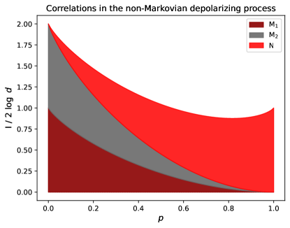
Figure 7: Correlations in the process shown in Fig. 6. Specifically in this process we always have $\mathrm{M}_{1}=\mathrm{M}_{2}$. For $p=0$ we have identity channels on both steps, implying $\mathrm{M}_{1}=\mathrm{M}_{2}=2\log d$ and $\mathrm{N}=0$, with $\mathrm{I}=\mathrm{M}=4\log d$. For $p>0$ there is information exchange with the environment in both steps, such that $\mathrm{M}<4\log d$, but part of the information lost in the first step is recovered in the second one, meaning $\mathrm{N}>0$. For $p=1$ if we input states $\rho_{1}$ and $\rho_{2}$ in the first and second steps, we obtain, respectively, $\tilde{\mathbb{I}}$ and $\rho_{1}$ as outputs, such that $\mathrm{M}_{1}=\mathrm{M}_{2}=0$, as each output is uncorrelated with its input. However, since the second output is maximally correlated with the first input, we still have information propagating in time through the environment, implying this is a highly non-Markovian process, with $\mathrm{I}=\mathrm{N}=2\log d$.

From the definitions of Eqs. (31) to (38) and the discussion of Sec. 2 we can see that

$$0\leq\mathrm{I}\leq 4\log d,$$ (43)

$$0\leq\mathrm{M}_{1}\leq 2\log d,$$ (44)

$$0\leq\mathrm{M}_{2}\leq 2\log d,$$ (45)

$$0\leq\mathrm{M}\leq 4\log d,$$ (46)

$$0\leq\mathrm{N}\leq 4\log d.$$ (47)

The saturation of the upper bound of the four first quantities above is achieved, for example, in the dynamics of Figs. 6 and 7 for $p=0$. The maximum possible value for $\mathrm{N}$ will be later discussed in more detail. Notice that the additive property of Eq. (40) implies

$$\mathrm{M}_{1}+\mathrm{M}_{2}+\mathrm{N}\leq 4\log d.$$ (48)

This means that Markovian and non-Markovian correlations limit the existence of one another, so that they cannot vary independently within their ranges. In particular, if $\mathrm{M}_{1}=\mathrm{M}_{2}=2\log d$ we must then necessarily have $\mathrm{N}=0$, an example of which we saw in Fig. 7.

Nevertheless, Eq. (48) does not carry all the physical properties of information exchange we expect the process to have. Consider, for example, a scenario in which $\mathrm{M}_{1}=2\log d$ and $\mathrm{M}_{2}=0$. From Eq. (48) we have $\mathrm{N}\leq 2\log d$, so we could say that it is still possible for the process to have some non-Markovianity. However, notice that $\mathrm{M}_{1}=2\log d$ implies that the first step of the dynamics is a unitary on the system alone, so the system does not exchange with the environment any information that could be recovered in the second step, and we must necessarily have $\mathrm{N}=0$. Analogously, in an opposite scenario where $\mathrm{M}_{1}=0$ and $\mathrm{M}_{2}=2\log d$, the system does not exchange information with the environment in the second step, so it cannot recover any information that was lost in the first one, also implying $\mathrm{N}=0$. This means that both $\mathrm{M}_{1}$ and $\mathrm{M}_{2}$ should somehow individually provide upper bounds to $\mathrm{N}$.

To obtain such bounds we proceed as in Eqs. (21) to (25), that is,

$$\mathrm{N} =S_{\mathrm{A}\mathrm{B}}+S_{\mathrm{C}\mathrm{D}}-S_{\mathrm{A}\mathrm{B}\mathrm{C}\mathrm{D}}$$ (49)

$$\leq 2S_{\mathrm{A}\mathrm{B}}$$ (50)

$$=2\quantity(S_{\mathrm{A}}+S_{\mathrm{B}}-\mathrm{M}_{1})$$ (51)

$$\leq 2\quantity(2\log d-\mathrm{M}_{1}),$$ (52)

and also

$$\mathrm{N} =S_{\mathrm{A}\mathrm{B}}+S_{\mathrm{C}\mathrm{D}}-S_{\mathrm{A}\mathrm{B}\mathrm{C}\mathrm{D}}$$ (53)

$$\leq 2S_{\mathrm{C}\mathrm{D}}$$ (54)

$$\leq 2\quantity(2\log d-\mathrm{M}_{2}).$$ (55)

This way, after defining the complements of the Markovian correlations $\overline{\mathrm{M}}_{j}\coloneqq 2\log d-\mathrm{M}_{j}$, we obtain a set of conditions describing how the Markovianity on each step individually limits the non-Markovianity of the process,

$$\mathrm{N}\leq\begin{cases}&2\overline{\mathrm{M}}_{1},\\ &2\overline{\mathrm{M}}_{2}.\end{cases}$$ (56)

By adding these conditions and dividing by two we recover Eq. (48). However, these more detailed bounds go beyond Eq. (48) in that they show how the presence of non-Markovian correlations require information exchange between system and environment in both steps.

Nevertheless, the conditions in Eq. (56) are still not the end of the story. This is because the time-ordering condition of Eq. (29) was not used in their derivation, therefore Eq. (56) is valid even for process matrices without a definite causal order. Notice that Eq. (29) implies $S_{\mathrm{A}\mathrm{B}\mathrm{C}}=S_{\mathrm{A}\mathrm{B}}+\log d$, so we have

$$\mathrm{N} =S_{\mathrm{A}\mathrm{B}}+S_{\mathrm{C}\mathrm{D}}-S_{\mathrm{A}\mathrm{B}\mathrm{C}\mathrm{D}}$$ (57)

$$=S_{\mathrm{A}\mathrm{B}\mathrm{C}}-\log d+S_{\mathrm{C}\mathrm{D}}-S_{\mathrm{A}\mathrm{B}\mathrm{C}\mathrm{D}}$$ (58)

$$\leq S_{\mathrm{D}}-\log d+S_{\mathrm{C}\mathrm{D}}$$ (59)

$$\leq S_{\mathrm{C}\mathrm{D}}$$ (60)

$$\leq\overline{\mathrm{M}}_{2},$$ (61)

where we used $S_{\mathrm{A}\mathrm{B}\mathrm{C}}-S_{\mathrm{A}\mathrm{B}\mathrm{C}\mathrm{D}}\leq S_{\mathrm{D}}$, implied by Eq. (26)$,S_{\mathrm{D}}\leq\log d$ and $S_{\mathrm{C}\mathrm{D}}\leq 2\log d-\mathrm{M}_{2}$. The set of conditions is then updated to

$$\mathrm{N}\leq\begin{cases}&2\overline{\mathrm{M}}_{1},\\ &\leavevmode\nobreak\ \leavevmode\nobreak\ \overline{\mathrm{M}}_{2}.\end{cases}$$ (62)

Such limitations to the non-Markovianity of any two-step process have several important implications. First, notice that $\mathrm{N}\leq 2\log d-\mathrm{M}_{2}\leq 2\log d$, so we can rewrite the range of $\mathrm{N}$ as

$$0\leq\mathrm{N}\leq 2\log d.$$ (63)

This means that, despite there being states in $\mathcal{B}(\mathcal{H}_{\mathrm{A}}\otimes\mathcal{H}_{\mathrm{B}}\otimes\mathcal{H}_{\mathrm{C}}\otimes\mathcal{H}_{\mathrm{D}})$ for which $2\log d<\mathrm{I}(\mathrm{A}\mathrm{B}:\mathrm{C}\mathrm{D})\leq 4\log d$, these are not Choi states of two-step process tensors, as they do not satisfy the time-ordering conditions of Eqs. (29) and (30). When restricted to the set of states that do satisfy such conditions, the maximum possible value for $\mathrm{I}(\mathrm{A}\mathrm{B}:\mathrm{C}\mathrm{D})$ is actually $2\log d$. An example of a process with this maximum non-Markovianity is that of Fig. 6 with $p=1$, where $\mathrm{M}_{1}=\mathrm{M}_{2}=0$. Importantly, while the condition $\mathrm{M}_{2}=0$ is necessary for $\mathrm{N}=2\log d$, we could still have $0<\mathrm{M}_{1}\leq\log d$, an example of which is shown in Fig. 8.

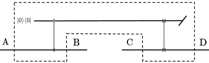
Figure 8: Maximally non-Markovian process with Markovian correlations in the first step. The first interaction is a CNOT with control on the system and target on the environment initially in the pure state $\ket{0}$. The second step is a SWAP between system and environment. The Choi state for this dynamics is $\Phi_{\mathrm{A}\mathrm{B}\mathrm{D}}\otimes\tilde{\mathbb{I}}_{\mathrm{C}}$, where $\Phi_{\mathrm{A}\mathrm{B}\mathrm{D}}$ is a maximally entangled tripartite state, which means we have $\mathrm{M}_{1}=\log d$, $\mathrm{M}_{2}=0$ and $\mathrm{N}=2\log d$. Upon inputting the states $\rho_{1}$ and $\rho_{2}$ to this process, we have the state $\rho_{1}$ teleported to the Bell basis of the joint output space $\mathrm{B}\mathrm{D}$. Considering each output individually, we have two classical copies of $\rho_{1}$, that is, $\rho_{1}$ dephased in the computational basis.

More generally, we could say that a process that has high Markovianity in some step has necessarily low non-Markovianity, that is,

$$\mathrm{M}_{1}\geq 2\log d-\varepsilon\implies\mathrm{N}\leq 2\varepsilon,$$ (64)

$$\mathrm{M}_{2}\geq 2\log d-\varepsilon\implies\mathrm{N}\leq\varepsilon.$$ (65)

On the other hand, a highly non-Markovian process is necessarily low in the Markovianity of its second step, but could still have medium Markovianity in the first one

$$\mathrm{N}\geq 2\log d-2\varepsilon\implies\begin{cases}&\mathrm{M}_{1}\leq\log d+\varepsilon,\\ &\mathrm{M}_{2}\leq 2\varepsilon.\end{cases}$$ (66)

Another relevant feature brought by Eq. (62) is that the interplay between Markovian and non-Markovian correlations is not symmetric. To see this, we rewrite the conditions in Eq. (62) as $\mathrm{M}_{1}\leq 2\log d-\mathrm{N}/2$ and $\mathrm{M}_{2}\leq 2\log d-\mathrm{N}$, which implies

$$\mathrm{M}\leq 4\log d-\frac{3}{2}\mathrm{N},$$ (67)

that is, for a process to have a given amount $\mathrm{N}$ of non-Markovianity it must “pay a price” in Markovianity of at least $3\mathrm{N}/2$. Alternatively, in terms of the total correlations of the process, we may write

$$\mathrm{I}\leq 4\log d-\frac{1}{2}\mathrm{N}.$$ (68)

This means that the only two-step processes with maximum total correlations are those with local unitaries on the system in both steps, so that they have maximum Markovian correlations and zero non-Markovian correlations, like in the example of Fig. 6 with $p=0$. On the other hand, a process with maximum non-Markovianity has at most $3\log d$ of total correlations, as in the example of Fig. 8. More generally, for a two-step process to approach the upper bound of $4\log d$ on total correlations it must have as little non-Markovianity as possible,

$$\mathrm{I}\geq 4\log d-\varepsilon\implies\mathrm{N}\leq 2\varepsilon.$$ (69)

Oppositely, any highly non-Markovian process has its total correlations limited to about $3\log d$,

$$\mathrm{N}\geq 2\log d-2\varepsilon\implies\mathrm{I}\leq 3\log d+\varepsilon.$$ (70)

In summary, we have discussed how the physical properties of information exchange and time-ordering of the processes give rise to fundamental relations between the Markovian and non-Markovian correlations of any two-step quantum process. The mathematical constraints imposed by these properties allowed us to derive the conditions of Eq. (62). These, in turn, provided a general upper bound to non-Markovian correlations and revealed that non-Markovianity is undesirable if one seeks a two-step process with a large amount of total correlations. Now, we follow to Sec. 4, where all these relevant results are generalized to the $n$-step scenario.

4 Temporal correlations in general multi-time quantum processes

We begin by defining the descriptor of the dynamics and its Choi state. We assume the most general multi-time quantum process to be described by an $n$-step process tensor, defined as following.

Definition 1.

An $n$-step process tensor $\mathcal{T}_{n}:\mathcal{B}(\mathcal{H}_{\mathrm{i}_{0}})\otimes\mathcal{B}^{2}(\mathcal{H}_{\mathrm{o}_{1}},\mathcal{H}_{\mathrm{i}_{1}})\otimes\cdots\otimes\mathcal{B}^{2}(\mathcal{H}_{\mathrm{o}_{n-1}},\mathcal{H}_{\mathrm{i}_{n-1}})\to\mathcal{B}(\mathcal{H}_{\mathrm{o}_{n}})$ is a multi-linear, completely positive, trace-preserving and time-ordered mapping from an input state $\rho\in\mathcal{B}(\mathcal{H}_{\mathrm{i}_{0}})$ and a sequence $\{\mathcal{M}_{j}\}_{j=1}^{n-1}$ of control operations $\mathcal{M}_{j}:\mathcal{B}(\mathcal{H}_{\mathrm{o}_{j}})\to\mathcal{B}(\mathcal{H}_{\mathrm{i}_{j}})$ to a final state $\rho^{\prime}\in\mathcal{B}(\mathcal{H}_{\mathrm{o}_{n}})$.

Noteworthy, it is also possible to use a process tensor to describe a dynamics in which system and environment are initially correlated. In this case, $\mathcal{T}_{n}$ will be a mapping from the control operations to the final state of the system. Despite these slight different conventions, the results we will derive should also hold in those cases with small adaptations.

Importantly, the process tensor $\mathcal{T}_{n}$ may be equivalently seen as a time-ordered mapping from a sequence of inputs to a sequence of outputs, that is, $\mathcal{T}_{n}:\mathcal{B}(\mathcal{H}_{\mathrm{i}_{0}}\otimes\cdots\otimes\mathcal{H}_{\mathrm{i}_{n-1}})\to\mathcal{B}(\mathcal{H}_{\mathrm{o}_{1}}\otimes\cdots\otimes\mathcal{H}_{\mathrm{o}_{n}})$. With this in mind, we define its Choi state.

Definition 2.

The Choi state $\Upsilon^{\mathcal{T}_{n}}\in\mathcal{B}(\mathcal{H}_{\mathrm{i}_{0}}\otimes\mathcal{H}_{\mathrm{o}_{1}}\otimes\cdots\otimes\mathcal{H}_{\mathrm{i}_{n-1}}\otimes\mathcal{H}_{\mathrm{o}_{n}})$ of the process tensor $\mathcal{T}_{n}$ is defined as

$$\Upsilon^{\mathcal{T}_{n}}\coloneqq\quantity(\bigotimes_{j=1}^{n}\mathcal{I}_{\mathrm{i}_{j-1}}\otimes\mathcal{T}_{n})\quantity(\bigotimes_{j=1}^{n}\Phi_{\mathrm{i}_{j-1},\mathrm{i}_{j-1}}).$$ (71)

This definition is a straightforward generalization of Eq. (28). Also, the circuit generating such state is an extension of that shown in Fig. 5. Eqs. (29) and (30) are generalized as follows.

Remark 1.

In terms of the Choi state, the trace-preservation and time-ordering properties of the process are given by the hierarchy of trace conditions

$$\tr_{\mathrm{o}_{j}}\quantity[\Upsilon_{1:j}^{\mathcal{T}_{2}}]=\Upsilon_{1:j-1}^{\mathcal{T}_{2}}\otimes\tilde{\mathbb{I}}_{\mathrm{i}_{j-1}},$$ (72)

for all $1\leq j\leq n$, where

$$\Upsilon_{1:j}^{\mathcal{T}_{2}}\coloneqq\tr_{j+1:n}\quantity[\Upsilon^{\mathcal{T}_{2}}],$$ (73)

and $\tr_{j+1:n}$ is the trace over the subspaces $\{\mathrm{i}_{j},\mathrm{o}_{j+1},\cdots,\mathrm{i}_{n-1},\mathrm{o}_{n}\}$.

Now, we follow to the definition of the correlation quantifiers in the $n$-step scenario.

Definition 3.

The total correlations $\mathrm{I}$, Markovian correlations in the $j$-th step $\mathrm{M}_{j}$, total Markovian correlations $\mathrm{M}$, and non-Markovian correlations $\mathrm{N}$ of the $n$-step process tensor $\mathcal{T}_{n}$ are respectively defined as

$$\mathrm{I}(\mathcal{T}_{n})\coloneqq\mathrm{I}(\mathrm{i}_{0}:\mathrm{o}_{1}:\cdots:\mathrm{i}_{n-1}:\mathrm{o}_{n})_{\Upsilon^{\mathcal{T}_{n}}},$$ (74)

$$\mathrm{M}_{j}(\mathcal{T}_{n})\coloneqq\mathrm{I}(\mathrm{i}_{j-1}:\mathrm{o}_{j})_{\Upsilon^{\mathcal{T}_{n}}},$$ (75)

$$\mathrm{M}(\mathcal{T}_{n})\coloneqq\sum_{j=1}^{n}\mathrm{M}_{j},$$ (76)

$$\mathrm{N}(\mathcal{T}_{n})\coloneqq\mathrm{I}(\mathrm{i}_{0}\mathrm{o}_{1}:\mathrm{i}_{1}\mathrm{o}_{2}:\cdots:\mathrm{i}_{n-1}\mathrm{o}_{n})_{\Upsilon^{\mathcal{T}_{n}}}.$$ (77)

These definitions are equivalent to those of Ref. [64]. This can be seen by writing the mutual information as the relative entropy between the state and the tensor product of its marginals, as shown in Eq. (7).

Alternatively, the above definitions may be written explicitly in terms of the von Neumann entropies of its Choi state’s marginals, which is done in the following Remark.

Remark 2.

Let $\tr_{\overline{\mathrm{A}}}\quantity[\Upsilon]$ denote the partial trace over all subsystems of $\Upsilon$ besides $\mathrm{A}$ and define

$$S_{\mathrm{i}_{j}}\coloneqq S\quantity(\tr_{\overline{\mathrm{i}_{j}}}\quantity[\Upsilon^{\mathcal{T}_{n}}]),$$ (78)

$$S_{\mathrm{o}_{j}}\coloneqq S\quantity(\tr_{\overline{\mathrm{o}_{j}}}\quantity[\Upsilon^{\mathcal{T}_{n}}]),$$ (79)

$$S_{j}\coloneqq S\quantity(\tr_{\overline{\mathrm{i}_{j-1}\mathrm{o}_{j}}}\quantity[\Upsilon^{\mathcal{T}_{n}}]),$$ (80)

$$S_{\overline{j}}\coloneqq S\quantity(\tr_{\mathrm{i}_{k-1}\mathrm{o}_{j}}\quantity[\Upsilon^{\mathcal{T}_{n}}])$$ (81)

and recalling Eq. (73),

$$S_{1:j}\coloneqq S\quantity(\Upsilon^{\mathcal{T}_{n}}_{1:j}).$$ (82)

Then, the correlation quantifiers may be rewritten as

$$\mathrm{I}=\sum_{j=1}^{n}\quantity(S_{\mathrm{i}_{j-1}}+S_{\mathrm{o}_{j}})-S_{1:n},$$ (83)

$$\mathrm{M}_{j}=S_{\mathrm{i}_{j-1}}+S_{\mathrm{o}_{j}}-S_{j},$$ (84)

$$\mathrm{M}=\sum_{j=1}^{n}\quantity(S_{\mathrm{i}_{j-1}}+S_{\mathrm{o}_{j}}-S_{j}),$$ (85)

$$\mathrm{N}=\sum_{j=1}^{n}S_{j}-S_{1:n}.$$ (86)

Importantly, by comparing the above equations we readily obtain the additive property

$$\mathrm{I}=\mathrm{M}+\mathrm{N}.$$ (87)

Finally, we also define the complement of $\mathrm{M}_{j}$,

$$\overline{\mathrm{M}_{j}}\coloneqq 2\log d-\mathrm{M}_{j}.$$ (88)

Having set the ground with the definitions, we now follow to the results.

Proposition 1.

For any (not necessarily time-ordered) process matrix $\mathcal{T}_{n}$, the following set of conditions holds,

$$\mathrm{N}\leq 2\sum_{j\neq k}\overline{\mathrm{M}_{j}},$$ (89)

for all $1\leq k\leq n$.

Proof.

From Eq. (26) we have

$$|S_{\overline{k}}-S_{k}|\leq S_{1:n},$$ (90)

which implies

$$S_{k}-S_{1:n}\leq S_{\overline{k}}.$$ (91)

Also, the subadditivity of von Neumann entropy $S_{\mathrm{AB}}\leq S_{\mathrm{A}}+S_{\mathrm{B}}$ [3, 4] yields

$$S_{\overline{k}}\leq\sum_{j\neq k}S_{j}.$$ (92)

Applying these to the non-Markovianity we obtain, for any $1\leq k\leq n$,

$$\mathrm{N} =\sum_{j=1}^{n}S_{j}-S_{1:n}$$ (93)

$$\leq\sum_{j\neq k}S_{j}+S_{\overline{k}}$$ (94)

$$=2\sum_{j\neq k}S_{j}$$ (95)

$$\leq 2\sum_{j\neq k}\overline{\mathrm{M}_{j}}.$$ (96)

∎

Example 1.

For a $4$-step process, the conditions of Prop. 1 are explicitly given by

$$\mathrm{N}\leq\begin{cases}&2\quantity(\overline{\mathrm{M}_{2}}+\overline{\mathrm{M}_{3}}+\overline{\mathrm{M}_{4}}),\\ &2\quantity(\overline{\mathrm{M}_{1}}+\overline{\mathrm{M}_{3}}+\overline{\mathrm{M}_{4}}),\\ &2\quantity(\overline{\mathrm{M}_{1}}+\overline{\mathrm{M}_{2}}+\overline{\mathrm{M}_{4}}),\\ &2\quantity(\overline{\mathrm{M}_{1}}+\overline{\mathrm{M}_{2}}+\overline{\mathrm{M}_{3}}).\end{cases}$$ (97)

Nevertheless, this set of conditions may be refined if we take the time-ordering of the process into account. This is done in the following Proposition.

Proposition 2.

For any $n$-step process tensor $\mathcal{T}_{n}$, the following set of conditions holds,

$$\mathrm{N}\leq 2\sum_{j<k}\overline{\mathrm{M}_{j}}+\sum_{j>k}\overline{\mathrm{M}_{j}},$$ (98)

for all $1\leq k\leq n$.

Proof.

The trace conditions of Eq. (72) imply

$$S_{1:k-1,\mathrm{i}_{k-1}}=S_{1:k-1}+\log d,$$ (99)

so we have

$$S_{1:k-1} =S_{1:k-1,\mathrm{i}_{k-1}}-\log d$$ (100)

$$\leq S_{1:k}+S_{\mathrm{o}_{k}}-\log d$$ (101)

$$\leq S_{1:k},$$ (102)

since $S_{1:k-1,\mathrm{i}_{k-1}}-S_{\mathrm{o}_{k}}\leq S_{1:k}$ holds from Eq. (26) and also $S_{\mathrm{o}_{k}}\leq\log d$. Then, we can write

$$S_{k}-S_{1:n} \leq S_{k}-S_{1:k}$$ (103)

$$\leq S_{1:k-1}$$ (104)

$$\leq\sum_{j<k}S_{j},$$ (105)

using $S_{k}-S_{1:k-1}\leq S_{1:k}$, again from Eq. (26), and subadditivity. Finally, for the non-Markovianity

$$\mathrm{N} =\sum_{j=1}^{n}S_{j}-S_{1:n}$$ (106)

$$=\sum_{j\neq k}S_{j}+\quantity(S_{k}-S_{1:n})$$ (107)

$$\leq\sum_{j\neq k}S_{j}+\sum_{j<k}S_{j}$$ (108)

$$=2\sum_{j<k}S_{j}+\sum_{j>k}S_{j}$$ (109)

$$\leq 2\sum_{j<k}\overline{\mathrm{M}_{j}}+\sum_{j>k}\overline{\mathrm{M}_{j}}.$$ (110)

∎

Example 2.

For a $4$-step process, the conditions of Prop. 2 are explicitly given by

$$\mathrm{N}\leq\begin{cases}&\overline{\mathrm{M}_{2}}+\overline{\mathrm{M}_{3}}+\overline{\mathrm{M}_{4}},\\ &2\overline{\mathrm{M}_{1}}+\overline{\mathrm{M}_{3}}+\overline{\mathrm{M}_{4}},\\ &2\overline{\mathrm{M}_{1}}+2\overline{\mathrm{M}_{2}}+\overline{\mathrm{M}_{4}},\\ &2\overline{\mathrm{M}_{1}}+2\overline{\mathrm{M}_{2}}+2\overline{\mathrm{M}_{3}}.\end{cases}$$ (111)

Having proved the set of conditions of Prop. 2, we now derive two theorems concerning non-Markovianity of general multi-time quantum processes.

Theorem 1.

The maximum non-Markovianity $\mathrm{N}$ of any $n$-step process tensor $\mathcal{T}_{n}$ is $2(n-1)\log d$.

Proof.

From the set of conditions in Prop. 2, choose $k=1$, yielding

$$\mathrm{N} \leq\sum_{j=2}^{n}\overline{\mathrm{M}_{j}}$$ (112)

$$=2(n-1)\log d-\sum_{j=2}^{n}\mathrm{M}_{j}$$ (113)

$$\leq 2(n-1)\log d.$$ (114)

∎

Example 3.

Consider the $n$-step process associated to the Choi state

$$\Upsilon^{\mathcal{T}_{n}}=\tilde{\mathbb{I}}_{\mathrm{o}_{i}}\otimes\Phi_{\mathrm{i}_{0}\mathrm{o}_{2}}\otimes\Phi_{\mathrm{i}_{1}\mathrm{o}_{3}}\otimes\cdots\otimes\Phi_{\mathrm{i}_{n-2}\mathrm{o}_{n}}\otimes\tilde{\mathbb{I}}_{\mathrm{i}_{n-1}}.$$ (115)

This is a generalization to $n$-steps of the process of Fig. 6 with $p=1$, such that the output of the $(j+1)$-th step is equal to the input of the $j$-th step. The first output is $\tilde{\mathbb{I}}$ and the last input is discarded. It is straightforward to show that for this process

$$\mathrm{N}=2(n-1)\log d,$$ (116)

that is, it is maximally non-Markovian. Also, we have that $\mathrm{M}=0$, such that $\mathrm{I}=\mathrm{N}$.

Now, we derive how the non-Markovianity upper bounds the maximum possible Markovianity of a given process.

Theorem 2.

For any $n$-step process tensor $\mathcal{T}_{n}$ it holds that

$$\mathrm{M}\leq 2n\log d-\frac{2^{n}-1}{2^{n}-2}\mathrm{N}.$$ (117)

Proof.

Take each condition from Prop. 2, multiply both sides by $2^{n-k}$ and sum for every $1\leq k\leq n$, yielding

$$\sum_{k=1}^{n}2^{n-k}\mathrm{N}\leq\sum_{k=1}^{n}2^{n-k}\quantity[2\sum_{j=1}^{k-1}\overline{\mathrm{M}_{j}}+\sum_{j=k+1}^{n}\overline{\mathrm{M}_{j}}],$$ (118)

and after some tedious calculations we obtain

$$\quantity(2^{n}-1)\mathrm{N} \leq\quantity(2^{n}-2)\sum_{j=1}^{n}\overline{\mathrm{M}_{j}}$$ (119)

$$=\quantity(2^{n}-2)\quantity(2n\log d-\mathrm{M}),$$ (120)

which, after isolating $\mathrm{M}$, results in the inequality of the theorem. ∎

Alternatively, we may rewrite this result showing how the non-Markovianity limits the total correlations of the process.

Theorem 2^′.

For any $n$-step process tensor $\mathcal{T}_{n}$ it holds that

$$\mathrm{I}\leq 2n\log d-\frac{1}{2^{n}-2}\mathrm{N}.$$ (121)

Proof.

Take Thm. 2 and add $\mathrm{N}$ to both sides. In the LHS we use $\mathrm{M}+\mathrm{N}=\mathrm{I}$, obtaining the inequality of the theorem. ∎

This last theorem shows that a non-Markovian process cannot have maximum total correlations. However, the ”price” paid in total correlations to have a given amount of non-Markovianity decays exponentially with the number of steps of the process. This implies that a highly non-Markovian process with many steps might achieve an amount of total correlations relatively close to that of a unitary process with a similar number of steps.

5 Conclusions

We have shown how to establish useful bounds relating the different types of temporal correlations present in general multi-time quantum processes. We used the notion of information exchange between system and environment and the time-ordering of the process to prove a set of inequalities relating Markovian correlations in individual steps to the global non-Markovianity. From these, we derived relevant results concerning the correlation quantifiers, like the maximum possible value for the non-Markovianity and how it limits the total correlations of the process depending on its number of steps. Given the importance of dealing with temporal correlations in quantum processes, we hope these results help us pave the way towards a deeper understanding of informational flow in quantum systems, perhaps leading to significant improvements of state-of-art quantum information processing technologies.

References

- Breuer and Petruccione [2002] Heinz-Peter Breuer and Francesco Petruccione. The theory of open quantum systems. Oxford University Press, USA, 2002.
- Rivas and Huelga [2012] Angel Rivas and Susana F Huelga. Open quantum systems, volume 10. Springer, 2012.
- Nielsen and Chuang [2010] Michael A Nielsen and Isaac L Chuang. Quantum computation and quantum information. Cambridge university press, 2010.
- Wilde [2013] Mark M Wilde. Quantum information theory. Cambridge university press, 2013.
- Preskill [2018] John Preskill. Quantum Computing in the NISQ era and beyond. Quantum, 2:79, August 2018. ISSN 2521-327X. doi: 10.22331/q-2018-08-06-79.
- Rivas et al. [2014] Ángel Rivas, Susana F Huelga, and Martin B Plenio. Quantum non-markovianity: characterization, quantification and detection. Reports on Progress in Physics, 77(9):094001, 2014. doi: 10.1088/0034-4885/77/9/094001.
- Breuer et al. [2016] Heinz-Peter Breuer, Elsi-Mari Laine, Jyrki Piilo, and Bassano Vacchini. Colloquium: Non-markovian dynamics in open quantum systems. Rev. Mod. Phys., 88:021002, Apr 2016. doi: 10.1103/RevModPhys.88.021002.
- de Vega and Alonso [2017] Inés de Vega and Daniel Alonso. Dynamics of non-markovian open quantum systems. Rev. Mod. Phys., 89:015001, Jan 2017. doi: 10.1103/RevModPhys.89.015001.
- Li et al. [2018] Li Li, Michael JW Hall, and Howard M Wiseman. Concepts of quantum non-markovianity: A hierarchy. Physics Reports, 759:1–51, 2018. doi: 10.1016/j.physrep.2018.07.001.
- Pollock et al. [2018a] Felix A Pollock, César Rodríguez-Rosario, Thomas Frauenheim, Mauro Paternostro, and Kavan Modi. Non-markovian quantum processes: Complete framework and efficient characterization. Physical Review A, 97(1):012127, 2018a. doi: 10.1103/PhysRevA.97.012127.
- Milz et al. [2020a] Simon Milz, Fattah Sakuldee, Felix A Pollock, and Kavan Modi. Kolmogorov extension theorem for (quantum) causal modelling and general probabilistic theories. Quantum, 4:255, 2020a. doi: 10.22331/q-2020-04-20-255.
- Pollock et al. [2018b] Felix A Pollock, César Rodríguez-Rosario, Thomas Frauenheim, Mauro Paternostro, and Kavan Modi. Operational markov condition for quantum processes. Physical review letters, 120(4):040405, 2018b. doi: 10.1103/PhysRevLett.120.040405.
- Milz et al. [2019] Simon Milz, MS Kim, Felix A Pollock, and Kavan Modi. Completely positive divisibility does not mean markovianity. Physical review letters, 123(4):040401, 2019. doi: 10.1103/PhysRevLett.123.040401.
- Taranto et al. [2019a] Philip Taranto, Felix A Pollock, Simon Milz, Marco Tomamichel, and Kavan Modi. Quantum markov order. Physical Review Letters, 122(14):140401, 2019a. doi: 10.1103/PhysRevLett.122.140401.
- Taranto et al. [2019b] Philip Taranto, Simon Milz, Felix A Pollock, and Kavan Modi. Structure of quantum stochastic processes with finite markov order. Physical Review A, 99(4):042108, 2019b. doi: 10.1103/PhysRevA.99.042108.
- Figueroa-Romero et al. [2019] Pedro Figueroa-Romero, Kavan Modi, and Felix A Pollock. Almost markovian processes from closed dynamics. Quantum, 3:136, 2019. doi: 10.22331/q-2019-04-30-136.
- Milz et al. [2020b] Simon Milz, Dario Egloff, Philip Taranto, Thomas Theurer, Martin B Plenio, Andrea Smirne, and Susana F Huelga. When is a non-markovian quantum process classical? Physical Review X, 10(4):041049, 2020b. doi: 10.1103/PhysRevX.10.041049.
- Milz et al. [2021] Simon Milz, Cornelia Spee, Zhen-Peng Xu, Felix A Pollock, Kavan Modi, and Otfried Gühne. Genuine multipartite entanglement in time. SciPost Physics, 10(6):141, 2021. doi: 10.21468/SciPostPhys.10.6.141.
- Taranto et al. [2021] Philip Taranto, Felix A Pollock, and Kavan Modi. Non-markovian memory strength bounds quantum process recoverability. npj Quantum Information, 7(1):149, 2021. doi: 10.1038/s41534-021-00481-4.
- Figueroa-Romero et al. [2021a] Pedro Figueroa-Romero, Felix A Pollock, and Kavan Modi. Markovianization with approximate unitary designs. Communications Physics, 4(1):127, 2021a. doi: 10.1038/s42005-021-00629-w.
- Sakuldee et al. [2022] Fattah Sakuldee, Philip Taranto, and Simon Milz. Connecting commutativity and classicality for multitime quantum processes. Physical Review A, 106(2):022416, 2022. doi: 10.1103/PhysRevA.106.022416.
- Capela et al. [2022] Matheus Capela, Lucas C Céleri, Rafael Chaves, and Kavan Modi. Quantum markov monogamy inequalities. Physical Review A, 106(2):022218, 2022. doi: 10.1103/PhysRevA.106.022218.
- Taranto et al. [2023a] Philip Taranto, Thomas J Elliott, and Simon Milz. Hidden quantum memory: Is memory there when somebody looks? Quantum, 7:991, 2023a. doi: 10.22331/q-2023-04-27-991.
- Taranto et al. [2023b] Philip Taranto, Marco Túlio Quintino, Mio Murao, and Simon Milz. Characterising the hierarchy of multi-time quantum processes with classical memory. arXiv preprint arXiv:2307.11905, 2023b. doi: 10.48550/arXiv.2307.11905.
- van Kampen [1992] Nicolaas G van Kampen. Stochastic processes in physics and chemistry, volume 1. Elsevier, 1992.
- van Kampen [1998] Nicolaas G van Kampen. Remarks on non-markov processes. Brazilian Journal of Physics, 28:90–96, 1998. doi: 10.1590/S0103-97331998000200003.
- Jørgensen and Pollock [2019] Mathias R. Jørgensen and Felix A. Pollock. Exploiting the causal tensor network structure of quantum processes to efficiently simulate non-markovian path integrals. Phys. Rev. Lett., 123:240602, Dec 2019. doi: 10.1103/PhysRevLett.123.240602.
- Jørgensen and Pollock [2020] Mathias R. Jørgensen and Felix A. Pollock. Discrete memory kernel for multitime correlations in non-markovian quantum processes. Phys. Rev. A, 102:052206, Nov 2020. doi: 10.1103/PhysRevA.102.052206.
- Xiang et al. [2021] Liang Xiang, Zhiwen Zong, Ze Zhan, Ying Fei, Chongxin Run, Yaozu Wu, Wenyan Jin, Zhilong Jia, Peng Duan, Jianlan Wu, et al. Quantify the non-markovian process with intervening projections in a superconducting processor. arXiv preprint arXiv:2105.03333, 2021. doi: 10.48550/arXiv.2105.03333.
- Cygorek et al. [2022] Moritz Cygorek, Michael Cosacchi, Alexei Vagov, Vollrath Martin Axt, Brendon W Lovett, Jonathan Keeling, and Erik M Gauger. Simulation of open quantum systems by automated compression of arbitrary environments. Nature Physics, 18(6):662–668, 2022. doi: 10.1038/s41567-022-01544-9.
- Fowler-Wright et al. [2022] Piper Fowler-Wright, Brendon W. Lovett, and Jonathan Keeling. Efficient many-body non-markovian dynamics of organic polaritons. Phys. Rev. Lett., 129:173001, Oct 2022. doi: 10.1103/PhysRevLett.129.173001.
- Gribben et al. [2022] Dominic Gribben, Aidan Strathearn, Gerald E. Fux, Peter Kirton, and Brendon W. Lovett. Using the Environment to Understand non-Markovian Open Quantum Systems. Quantum, 6:847, October 2022. ISSN 2521-327X. doi: 10.22331/q-2022-10-25-847.
- Cygorek et al. [2023] Moritz Cygorek, Jonathan Keeling, Brendon W Lovett, and Erik M Gauger. Sublinear scaling in non-markovian open quantum systems simulations. arXiv preprint arXiv:2304.05291, 2023. doi: 10.48550/arXiv.2304.05291.
- Fux et al. [2023] Gerald E. Fux, Dainius Kilda, Brendon W. Lovett, and Jonathan Keeling. Tensor network simulation of chains of non-markovian open quantum systems. Phys. Rev. Res., 5:033078, Aug 2023. doi: 10.1103/PhysRevResearch.5.033078.
- Figueroa-Romero et al. [2021b] Pedro Figueroa-Romero, Kavan Modi, Robert J Harris, Thomas M Stace, and Min-Hsiu Hsieh. Randomized benchmarking for non-markovian noise. PRX Quantum, 2(4):040351, 2021b. doi: 10.1103/PRXQuantum.2.040351.
- Figueroa-Romero et al. [2022] Pedro Figueroa-Romero, Kavan Modi, and Min-Hsiu Hsieh. Towards a general framework of randomized benchmarking incorporating non-markovian noise. Quantum, 6:868, 2022. doi: 10.22331/q-2022-12-01-868.
- Figueroa-Romero et al. [2023] Pedro Figueroa-Romero, Miha Papič, Adrian Auer, Min-Hsiu Hsieh, Kavan Modi, and Inés de Vega. Operational markovianization in randomized benchmarking. arXiv preprint arXiv:2305.04704, 2023. doi: 10.48550/arXiv.2305.04704.
- Milz et al. [2018a] Simon Milz, Felix A Pollock, and Kavan Modi. Reconstructing non-markovian quantum dynamics with limited control. Physical Review A, 98(1):012108, 2018a. doi: 10.1103/PhysRevA.98.012108.
- White et al. [2020] Gregory AL White, Charles D Hill, Felix A Pollock, Lloyd CL Hollenberg, and Kavan Modi. Demonstration of non-markovian process characterisation and control on a quantum processor. Nature Communications, 11(1):6301, 2020. doi: 10.1038/s41467-020-20113-3.
- White et al. [2021] Gregory AL White, Felix A Pollock, Lloyd CL Hollenberg, Charles D Hill, and Kavan Modi. From many-body to many-time physics. arXiv preprint arXiv:2107.13934, 2021. doi: 10.48550/arXiv.2107.13934.
- White et al. [2022] Gregory AL White, Felix A Pollock, Lloyd CL Hollenberg, Kavan Modi, and Charles D Hill. Non-markovian quantum process tomography. PRX Quantum, 3(2):020344, 2022. doi: 10.1103/PRXQuantum.3.020344.
- White [2022] Gregory White. Characterization and control of non-markovian quantum noise. Nature Reviews Physics, 4(5):287–287, 2022. doi: 10.1038/s42254-022-00446-2.
- White et al. [2023] Gregory AL White, Kavan Modi, and Charles D Hill. Filtering crosstalk from bath non-markovianity via spacetime classical shadows. Physical Review Letters, 130(16):160401, 2023. doi: 10.1103/PhysRevLett.130.160401.
- Aloisio et al. [2023] Isobel A Aloisio, Gregory AL White, Charles D Hill, and Kavan Modi. Sampling complexity of open quantum systems. PRX Quantum, 4(2):020310, 2023. doi: 10.1103/PRXQuantum.4.020310.
- Strasberg [2019] Philipp Strasberg. Repeated interactions and quantum stochastic thermodynamics at strong coupling. Physical review letters, 123(18):180604, 2019. doi: 10.1103/PhysRevLett.123.180604.
- Figueroa-Romero et al. [2020] Pedro Figueroa-Romero, Kavan Modi, and Felix A Pollock. Equilibration on average in quantum processes with finite temporal resolution. Physical Review E, 102(3):032144, 2020. doi: 10.1103/PhysRevE.102.032144.
- Huang [2022] Zhiqiang Huang. Fluctuation theorems for multitime processes. Phys. Rev. A, 105:062217, Jun 2022. doi: 10.1103/PhysRevA.105.062217.
- Huang [2023] Zhiqiang Huang. Multiple entropy production for multitime quantum processes. Phys. Rev. A, 108:032217, Sep 2023. doi: 10.1103/PhysRevA.108.032217.
- Dowling et al. [2023a] Neil Dowling, Pedro Figueroa-Romero, Felix A Pollock, Philipp Strasberg, and Kavan Modi. Relaxation of multitime statistics in quantum systems. Quantum, 7:1027, 2023a. doi: 10.22331/q-2023-06-01-1027.
- Dowling et al. [2023b] Neil Dowling, Pedro Figueroa-Romero, Felix A Pollock, Philipp Strasberg, and Kavan Modi. Equilibration of multitime quantum processes in finite time intervals. SciPost Physics Core, 6(2):043, 2023b. doi: 10.21468/SciPostPhysCore.6.2.043.
- Guo et al. [2020] Chu Guo, Kavan Modi, and Dario Poletti. Tensor-network-based machine learning of non-markovian quantum processes. Phys. Rev. A, 102:062414, Dec 2020. doi: 10.1103/PhysRevA.102.062414.
- Huang and Guo [2023] Zhiqiang Huang and Xiao-Kan Guo. Leggett-garg inequalities for multitime processes. arXiv preprint arXiv:2211.13396, 2023. doi: 10.48550/arXiv.2211.13396.
- Butler et al. [2023] Eoin P Butler, Gerald Fux, Brendon W Lovett, Jonathan Keeling, and Paul R Eastham. Optimizing performance of quantum operations with non-markovian decoherence: the tortoise or the hare? arXiv preprint arXiv:2303.16002, 2023. doi: 10.48550/arXiv.2303.16002.
- Chiribella et al. [2008] G. Chiribella, G. M. D’Ariano, and P. Perinotti. Quantum circuit architecture. Phys. Rev. Lett., 101:060401, Aug 2008. doi: 10.1103/PhysRevLett.101.060401.
- Chiribella et al. [2009] Giulio Chiribella, Giacomo Mauro D’Ariano, and Paolo Perinotti. Theoretical framework for quantum networks. Physical Review A, 80(2):022339, 2009. doi: 10.1103/PhysRevA.80.022339.
- Costa and Shrapnel [2016] Fabio Costa and Sally Shrapnel. Quantum causal modelling. New Journal of Physics, 18(6):063032, jun 2016. doi: 10.1088/1367-2630/18/6/063032.
- Costa et al. [2018] Fabio Costa, Martin Ringbauer, Michael E. Goggin, Andrew G. White, and Alessandro Fedrizzi. Unifying framework for spatial and temporal quantum correlations. Phys. Rev. A, 98:012328, Jul 2018. doi: 10.1103/PhysRevA.98.012328.
- Milz et al. [2018b] Simon Milz, Felix A Pollock, Thao P Le, Giulio Chiribella, and Kavan Modi. Entanglement, non-markovianity, and causal non-separability. New Journal of Physics, 20(3):033033, 2018b. doi: 10.1088/1367-2630/aaafee.
- Nery et al. [2021] Marcello Nery, Marco Túlio Quintino, Philippe Allard Guérin, Thiago O. Maciel, and Reinaldo O. Vianna. Simple and maximally robust processes with no classical common-cause or direct-cause explanation. Quantum, 5:538, September 2021. ISSN 2521-327X. doi: 10.22331/q-2021-09-09-538.
- Giarmatzi and Costa [2021] Christina Giarmatzi and Fabio Costa. Witnessing quantum memory in non-Markovian processes. Quantum, 5:440, April 2021. ISSN 2521-327X. doi: 10.22331/q-2021-04-26-440.
- Milz et al. [2022] Simon Milz, Jessica Bavaresco, and Giulio Chiribella. Resource theory of causal connection. Quantum, 6:788, 2022. doi: 10.22331/q-2022-08-25-788.
- Milz and Quintino [2023] Simon Milz and Marco Túlio Quintino. Transformations between arbitrary (quantum) objects and the emergence of indefinite causality. arXiv preprint arXiv:2305.01247, 2023. doi: 10.48550/arXiv.2305.01247.
- Berk et al. [2021] Graeme D Berk, Andrew JP Garner, Benjamin Yadin, Kavan Modi, and Felix A Pollock. Resource theories of multi-time processes: A window into quantum non-markovianity. Quantum, 5:435, 2021. doi: 10.22331/q-2021-04-20-435.
- Berk et al. [2023] Graeme D Berk, Simon Milz, Felix A Pollock, and Kavan Modi. Extracting quantum dynamical resources: Consumption of non-markovianity for noise reduction. npj Quantum Information, 9(1):104, 2023. doi: 10.1038/s41534-023-00774-w.
- Chitambar and Gour [2019] Eric Chitambar and Gilad Gour. Quantum resource theories. Rev. Mod. Phys., 91:025001, Apr 2019. doi: 10.1103/RevModPhys.91.025001.
- Verstraete and Verschelde [2002] Frank Verstraete and Henri Verschelde. On quantum channels. arXiv preprint quant-ph/0202124, 2002. doi: 10.48550/arXiv.quant-ph/0202124.
- Stinespring [1955] W Forrest Stinespring. Positive functions on c*-algebras. Proceedings of the American Mathematical Society, 6(2):211–216, 1955. doi: 10.2307/2032342.
- Araki and Lieb [1970] Huzihiro Araki and Elliott H Lieb. Entropy inequalities. Communications in Mathematical Physics, 18(2):160–170, 1970. doi: 10.1007/BF01646092.