On randomized estimators of the Hafnian of a nonnegative matrix

Abstract

We investigate the performance of two approximation algorithms for the Hafnian of a nonnegative square matrix, namely the Barvinok and Godsil-Gutman estimators. We observe that, while there are examples of matrices for which these algorithms fail to provide a good approximation, the algorithms perform surprisingly well for adjacency matrices of random graphs. In most cases, the Godsil-Gutman estimator provides a far superior accuracy. For dense graphs, however, both estimators demonstrate a slow growth of the variance. For complete graphs, we show analytically that the relative variance $\sigma/\mu$ grows as a square root of the size of the graph. Finally, we simulate a Gaussian Boson Sampling experiment using the Godsil-Gutman estimator and show that the technique used can successfully reproduce low-order correlation functions.

I Introduction

Counting the number of perfect matchings in a graph is a well-known computationally hard problem. The function that takes an adjacency matrix and counts the perfect matchings (possibly with weights), known as the Hafnian, appears in consideration of a model of quantum computation called Gaussian Boson Sampling (GBS) [1, 2]. In this model, a particular optical setup is used to produce samples from a probability distribution which is believed to be hard to reproduce classically. The hardness stems from the fact that calculating the probability of a particular measurement outcome requires the calculation of the abovementioned Hafnian of a matrix that depends on the outcome.

Recently, a series of GBS experiments demonstrated sampling beyond reach of classical computers [3, 4, 5, 6]. While the demonstration of quantum advantage is an important milestone for quantum technology, there is still a long way from an efficient non-classical sampler to a device that would assist in solving practical problems.

A proposed route to applications consists in using the sampler as an approximate solver for the densest subgraph problem and related problems [7, 8, 9, 10]. The kernel matrix of the Gaussian state is taken to be a rescaled adjacency matrix of the problem graph. That way, the detection events correspond to vertex subsets and their induced subgraphs. The probability of observing a particular event is proportional to the Hafnian of the induced subgraph, which is correlated with its density. Thus, the most likely samples are approximate solutions of the densest subgraph problem, or at least good starting points for a classical search algorithm.

Crucially, in all graph-related applications to date, the kernel matrix is nonnegative, meaning that all its elements are greater or equal than zero. As we show in this work, this restriction severely limits the advantage that one can possibly gain from using a boson sampler.

In Ref. [11], Quesada and Arrazola propose a method for classical simulation of GBS which relies on the calculation of conditional probabilities. As a special case, they consider the GBS setups which have nonnegative kernel matrices. For such matrices, the authors propose a classical simulation algorithm that does not necessarily use exponential time. The key element of this algorithm is a probabilistic method of estimating the Hafnian of a nonnegative matrix due to Barvinok [12].

In this work, we investigate the behavior of the Barvinok estimator and a related method known as the Godsil-Gutman estimator [13]. On the one hand, we find that neither enables an approximate polynomial-time simulation for all nonnegative kernels simply because both estimators have exponential variance for certain matrices. We also find that the Godsil-Gutman estimator demonstrates a far superior performance in terms of variance. On the other hand, we conduct numerical experiments with both estimators for the adjacency matrices of random graphs and observe that the relative variance of the estimator does not grow exponentially with the size of the matrix. Specifically, for the Godsil-Gutman estimator, the mean relative error grows monotonously with the density of the graph, and for the complete graph it grows merely as a square root of the size of the matrix, meaning that the number of samples required to obtain a good approximation grows very modestly as well.

The paper is structured as follows. In Section II, we derive an expression for the variance of the Barvinok and Godsil-Gutman estimators in terms of vertex cycle covers and provide the examples of graphs that do not admit a polynomial approximation by these estimators. In Section III, we study the variance of the estimators for the complete graph. In Section IV, we show the results of numerical investigations for random graphs. Finally, in Section V, we report on a classical simulation of Gaussian Boson Sampling with nonnegative kernels. Section VI contains concluding remarks.

II Randomized estimators of the Hafnian

The Hafnian of a symmetric, even-dimensional matrix $A\in\mathbb{C}^{2m\times 2m}$ is defined as follows:

$$\operatorname{Haf}A=\sum_{\pi\in PM(2m)}\prod_{(i,j)\in\pi}a_{ij}.$$ (1)

Here $\pi\in PM(2m)$ means that $\pi$ is a perfect matching of $2m$ objects. We will often treat $A$ as an adjacency matrix of a weighted graph with vertex set $V=\{1,...,2m\}$ and edge set $E\subseteq\{(i,j)|i,j\in V,i\neq j\}$.

The Hafnian of a nonnegative matrix admits the following randomized approximation algorithm. Let $W$ be a skew-symmetric matrix whose above-diagonal entries are i.i.d. random variables such that $\mathbb{E}w_{ij}=0$ and $\mathbb{E}w_{ij}^{2}=1$. Define $G=W\odot\sqrt{A}$, where by $\sqrt{A}$ we mean the element-wise square root. Then one can show that

$$\mu\equiv\mathbb{E}\det G=\operatorname{Haf}A,$$ (2)

where the expectation is taken over the random matrix entries $g_{ij}=w_{ij}\sqrt{a_{ij}}$. This is proven by expanding the determinant by definition and observing that the only terms which do not vanish upon taking the expected value are those where $g_{ij}$ only appear in the second power. Such terms precisely correspond to perfect matchings of the graph vertices.

To estimate $\operatorname{Haf}A$, we then simply repeat the sampling $N$ times, calculate the determinants, and take the sample mean. When $w_{ij}$ are sampled from the discrete uniform distribution on $\{-1,1\}$, we call this protocol the Godsil-Gutman estimator [13], when $w_{ij}$ are distributed from the standard normal distribution, we call it the Barvinok estimator [12]. An important difference occurs in the fourth moment: for the standard normal distribution, $\mathbb{E}w_{ij}^{4}=3$, while for the discrete uniform distribution, $\mathbb{E}w_{ij}^{4}=1$.

The accuracy of the estimator depends on the variance $\sigma^{2}=\operatorname{Var}\det G$. If we want to achieve multiplicative error $\epsilon$, then the standard error of the mean $\sigma/\sqrt{N}$ has to be of the order $\mu\epsilon$. In particular, if the relative standard deviation $\sigma/\mu$ scales exponentially with the size of the problem, then $N$ will also have to scale exponentially.

In the following we derive an expression for $\mathbb{E}\det G^{2}$ and for $\left(\mathbb{E}\det G\right)^{2}$ in terms of vertex covers of the corresponding graph, such that the vertex covers only consist of matchings and cycles of even length. We will say that a permutation $\pi\in S_{2m}$ matches vertices $i$ and $j$ if $\pi(i)=j$ and $\pi(j)=i$.

Proposition 1.

Let $\mathbb{E}w_{ij}^{3}=0,\mathbb{E}w_{ij}^{4}=\eta$. Then

$$\mathbb{E}(\det G)^{2}=\sum_{d}\eta^{|\mathrm{match}(d)|}6^{|\mathrm{cycle}(d)|}\prod_{\begin{subarray}{c}(i,j)\in\mathrm{match}(d)\\ (k,l)\in d\setminus\mathrm{match}(d)\end{subarray}}a_{ij}^{2}a_{kl}.$$ (3)

Here the sum is taken over all edge subsets $d\subseteq E$ that consist of matchings (disjoint edges) and cycles of even length, such that every vertex is adjacent to some edge in $d$; $\mathrm{match}(d)$ is the set of matchings in $d$; $\mathrm{cycle}(d)$ is the set of even-length cycles in $d$.

Proof.

The squared determinant is the product of two sums over permutations:

$$(\det G)^{2}=\left(\sum_{\pi\in S_{2m}}\operatorname{sgn}\pi\prod_{i=1}^{2m}g_{i\pi(i)}\right)\times\\ \times\left(\sum_{\pi^{\prime}\in S_{2m}}\operatorname{sgn}\pi^{\prime}\prod_{i^{\prime}=1}^{2m}g_{i^{\prime}\pi^{\prime}(i^{\prime})}\right).$$ (4)

The terms that will not vanish under taking the expected value are monomials in $g_{ij}$ in which all terms appear either in the second or in the fourth power. An element $g_{ij}$ appears four times if both permutations match vertices $i$ and $j$. In this situation, taking the expected value over this particular multiple yields a factor $\eta a_{ij}^{2}$ (the minus signs coming from the skew-symmetry of $G$ are eliminated here). A variable $g_{ij}$ can appear in the second power in the following cases:

1. Exactly one of the permutations matches vertices $i$ and $j$, and the other permutation matches vertices $i$ and $j$ to some other vertices;

2. The vertex $i$ has the same orbit of size $\geq 3$ under the actions of both $\pi$ and $\pi^{\prime}$, and either $\pi(i)=j$ or $\pi(j)=i$;

Indeed, suppose that $\pi$ matches $i,j$ but $\pi^{\prime}$ does not. Then if $\pi^{\prime}(i)=k$ but $\pi^{\prime}(k)\neq i$, then $g_{ik}$ necessarily comes in the first power and thus vanishes. If $\pi^{\prime}(i)=j$ but $\pi^{\prime}(j)\neq i$, then the total power of $g_{ij}$ is three, which vanishes under taking the expected value. Therefore $\pi^{\prime}$ also has to match $i$ to some vertex, and the same applies to vertex $j$.

Suppose now that neither permutation matches $i$ with $j$, but $\pi(i)=j$ and $\pi^{\prime}(i)=j$. Then if $\pi(j)=k\neq\pi^{\prime}(j)$, the term $g_{jk}$ appears in the first power and vanishes under the expected value. Therefore, $\pi^{2}(i)=(\pi^{\prime})^{2}(i)$. Continuing by induction, we find that the whole orbit of $i$ has to be same under both permutations. The same can be shown if $\pi^{\prime-1}(i)=j$, mutatis mutandis.

Let us now assign to each nonvanishing term an edge subset $d\ \subseteq E$, by adding an edge $i,j$ if either of the vertices is mapped to the other by either $\pi$ or $\pi^{\prime}$. Taken together with the adjacent vertices as a subgraph, this edge subset contains only pairwise vertex matchings and cycles. If a pair of permutations $\pi,\pi^{\prime}$ contains a shared cycle of odd length, then we can construct permutations $\tilde{\pi}$ and $\tilde{\pi}^{\prime}$ by reversing the direction of this cycle. Thus, we will have four pairs of permutations corresponding to the same subgraph. However, reversing the direction of the cycles add a factor of $(-1)$ to its contribution, which means that these terms will cancel each other. Therefore, the only relevant subgraphs consist of matchings and even cycles.

Suppose a cycle in $d$ traverses vertices $v_{1},...,v_{2k}$. There are only six ways two permutations can act on these vertices to form a cycle in $d$: they can match vertices in an alternating fashion in two different ways, or both permutations can cyclically shift the vertices $(v_{1},...,v_{2k})$ in either direction. Thus, each relevant subset $d$ appears in the sum exactly $6^{|\mathrm{cycle}(d)|}$ times. The cycle type of both permutations is the same, therefore $\operatorname{sgn}\pi=\operatorname{sgn}\pi^{\prime}$. Thus, collecting the terms and prefactors coming from the expectations of the fourth powers of $g_{ij}$, we arrive to the desired formula. ∎

Proposition 2.

In the definitions of Proposition 1, the following is true:

$$\operatorname{Haf}^{2}A=\sum_{d}2^{|\mathrm{cycle}(d)|}\prod_{\begin{subarray}{c}(i,j)\in\mathrm{match}(d)\\ (k,l)\in d\setminus\mathrm{match}(d)\end{subarray}}a_{ij}^{2}a_{kl}.$$ (5)

Proof.

Let us expand the squared Hafnian by defintion:

$$\operatorname{Haf}^{2}A=\left(\sum_{\pi\in PM(2m)}\prod_{(i,j)\in\pi}a_{ij}\right)\times\\ \times\left(\sum_{\pi^{\prime}\in PM(2m)}\prod_{(k,l)\in\pi^{\prime}}a_{kl}\right).$$ (6)

The union of edges of two perfect matchings consists entirely of disjoint edges and alternating cycles. Each alternating cycle can be formed in two ways. Thus, every edge subset $d$ corresponds to $2^{|\mathrm{cycle}(d)|}$ terms in the sum (6). ∎

These expressions for the moments of the determinant help us construct two examples of matrices. The first one gives an exponential relative deviation to the Barvinok estimator and zero relative deviation to the Godsil-Gutman estimator, the second one gives and exponential relative deviation to both estimators.

The first example is the following matrix:

$$A=\begin{pmatrix}0&1\\ 1&0\\ &&0&1\\ &&1&0\\ &&&&0&1\\ &&&&1&0\\ &&&&&&\ddots&\\ &&&&&&&0&1\\ &&&&&&&1&0\\ \end{pmatrix}$$ (7)

Clearly $\operatorname{Haf}A=1$, since this is the adjacency matrix of a graph which has exactly one perfect matching. The determinant of $G$ is equal to

$$\det G=g_{12}^{2}g_{34}^{2}\dots g_{2m-1,2m}^{2}.$$ (8)

The expected square of the determinant is

$$\mathbb{E}(\det G)^{2}=\mathbb{E}g_{12}^{4}g_{34}^{4}\dots g_{2m-1,2m}^{4}=\eta^{m}.$$ (9)

This means that the variance of the Barvinok determinant for $A$ is equal to $3^{m}-1$. The variance of the Godsil-Gutman determinant, on the other hand, is equal to zero.

The second example is the adjacency matrix of a graph consisting of a disjoint union of $k$ cycles of length four. Using (3), we quickly find that the variance of either estimator grows exponentially faster in $k$ than the squared mean. In general, if $\mathcal{G}$ is a connected graph whose adjacency matrix is such that $\sigma/\mu=r>1$, then the disjoint union of $k$ copies of this graph will yield a relative deviation equal to $r^{k}$.

The complex variants of the Hafnian estimator seem to suffer from all the same problems as their real counterparts. We can construct such estimators by taking $W$ to be a skew-Hermitian matrix and $g_{ij}$ to be complex random variables such that $\mathbb{E}w_{ij}=0$ and $\mathbb{E}|w_{ij}|^{2}=1$. This can be, e.g., a Gaussian random variable or a discrete distribution over the roots of unity, as used in Ref. [14] for estimating the permanent. The same example as above (disjoint union of cycles with length 4) will produce an estimate with an exponentially high relative deviation.

Finally, we note that for a random real variable with zero mean and unit variance, the fourth moment cannot be less that one. Therefore, one cannot improve on the Godsil-Gutman estimator in terms of variance simply by changing the distribution of $w_{ij}$.

III Godsil-Gutman estimator for complete graphs

Ref. [15] notes that the relative deviation of the Godsil-Gutman determinant is polynomial in size for complete graphs. Here we go further and show that it actually grows as a square root of the number of vertices. To do this, we use the theory of combinatorial species [16, 17]. It enables us to enumerate the edge subsets entering the expressions (3) and (5).

A species $F$ is a functor from the category of finite sets and bijections to itself. If $S$ is a finite set, then the elements of $F(S)$ are referred to as $F$-structures. For example, we can define a functor $\mathbf{Match}$ which maps a finite set to the set of all perfect matchings on that set. In this case, the perfect matchings are the $F$-structures.

With each species $F$ we can associate an exponential generating function:

$$F(x)=\sum_{n=0}^{\infty}\frac{1}{n!}|F(\{1,...,n\})|x^{n}.$$ (10)

The requirement that $F$ is a functor guarantees that the cardinality of $F(X)$ only depends on the cardinality of $X$.

Crucially, there is a correspondence between the operations on the species and operations on the generating functions. We will use two of these operations: product and substitution. Let $F,G$ be two species. The product species $F\cdot G$ is a functor that maps a set $U$ to the set

$$\bigsqcup_{S\subseteq U}F(S)\times G(U\setminus S).$$ (11)

The generating function of $F\cdot G$ is the product $F(x)G(x)$ of the corresponding generating functions. The substitution $F\circ G$ is a more complicated functor. The structures created by $F\circ G$ are partitions of the finite set, each endowed with a $G$-structure, forming together an $F$-structure. It acts on sets as follows:

$$(F\circ G)(S)=\bigsqcup_{\pi\in\mathrm{part}(S)}\left(F(\pi)\times\prod_{Y\in\pi}G(Y)\right).$$ (12)

The generating function of $F\circ G$ is $F(G(x))$.

Finally, we need to introduce the weighted sets and weighted species. Let $K$ be a ring. A $K$-weighted set is a pair $(S,w)$, where $S$ is a finite set, and $w:S\rightarrow K$ is a function called weight. Given two weighted sets $(A,u),(B,v)$, the product $A\times B$ can be equipped with a weight by setting $w((a,b))=u(a)\cdot v(b)$. The disjoint union $A\sqcup B$ can be equipped with a weight by taking the weights of the comprising subsets.

A weighted species is a functor from the category of finite sets and bijections to the category of weighted sets and weight-preserving bijections. Given a weighted species $F$, we can associate with it an exponential generating function with coefficients in $K$:

$$F(x)=\sum_{n=0}^{\infty}\frac{1}{n!}|F(\{1,...,n\})|_{w}x^{n}.$$ (13)

Here $|F(S)|_{w}=\sum_{x\in F(S)}w(x)$ is the weighted sum of the elements in $F(S)$. The operations on weighted species and their generating functions correspond to each other in exactly the same way as non-weighted species and their generating functions.

With this toolset at our disposal, we can construct a weighted species whose structures on $2m$-element sets are vertex covers consisting of matchings and cycles of even length, with weights equal to the coefficients in (3). All of these structures are present in a complete graph, so what we need is the sum of their weights. Thus, the coefficient before $x^{2m}$ in the generating function of this species will represent the second moment of the probabilistic estimator.

We consider the ring of real polynomials in one variable $\mathbb{R}[t]$ as the ring of weights. We will later set $t=\eta$ to account for the type of the estimator. Let us define the following functors (when weight is not specified, it is equal to one on all elements of the set):

1. $\mathbf{Pair}_{t}$ maps any two-element set to $(\{\bullet\},t)$, where $\{\bullet\}$ is a singleton set. All other sets are mapped to the empty set. The generating function is equal to $\mathbf{Pair}_{t}(x)=\frac{tx^{2}}{2}$.

2. $\mathbf{Exp}$ maps any set to the singleton set. Its generating function is equal to $e^{x}$.

3. $\mathbf{Cycle}$ maps any set of size $4+2k$ to the set of all cyclic orderings on this set (up to the inverse), and all other sets to the empty set. Its generating function is equal to

   $$\mathbf{Cycle}(x)=\frac{1}{2}\left(\frac{3!x^{4}}{4!}+\frac{5!x^{6}}{6!}+...\right)=\\ =-\frac{1}{4}\log(1-x^{2})-\frac{x^{2}}{4}.$$ (14)

   We will need a weighted functor $6\mathbf{Cycle}$, such that the weights of all elements of the output sets are equal to 6. Its generating function is thus equal to $-\frac{3}{2}\log(1-x^{2})-\frac{3x^{2}}{2}$.

We will construct two more functors: $\mathbf{Match}_{t}$, which maps a set to its perfect matchings with weight $t$ raised to the power of the size of the matching, and $\mathbf{CycleCover}$, which maps a set to the set of its covers with cycles of even length.

Since every subgraph involved in (3) consists of a disjoint union of matchings and cycle covers, the subgraphs for the complete graph are generated by the functor $\mathbf{Match}_{t}\cdot\mathbf{CycleCover}$. Both the perfect matchings and cycle covers of a set can be thought of as partitions of the set together with the corresponding structure on each part. In terms of species, this means that $\mathbf{Match}_{t}=\mathbf{Exp}\circ\mathbf{Pair}_{t}$ and $\mathbf{CycleCover}=\mathbf{Exp}\circ 6\mathbf{Cycle}$. Altogether this means that the generating function for the second moments (3) is the following:

$$f(x,t)=e^{\frac{tx^{2}}{2}}e^{-\frac{3}{2}\log(1-x^{2})-\frac{3x^{2}}{2}}=\frac{\exp(\frac{(t-3)x^{2}}{2})}{(1-x^{2})^{3/2}}.$$ (15)

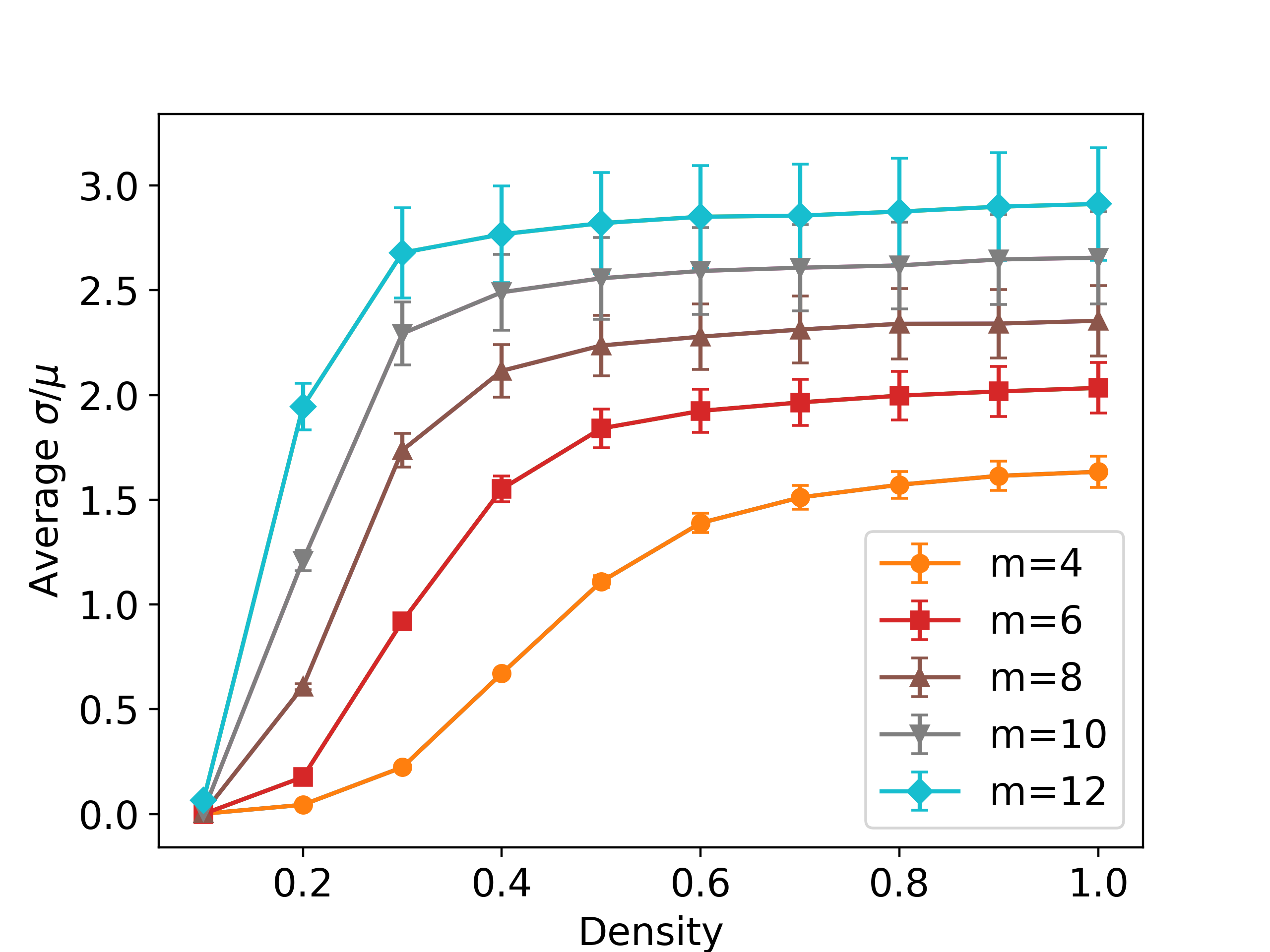
(a)

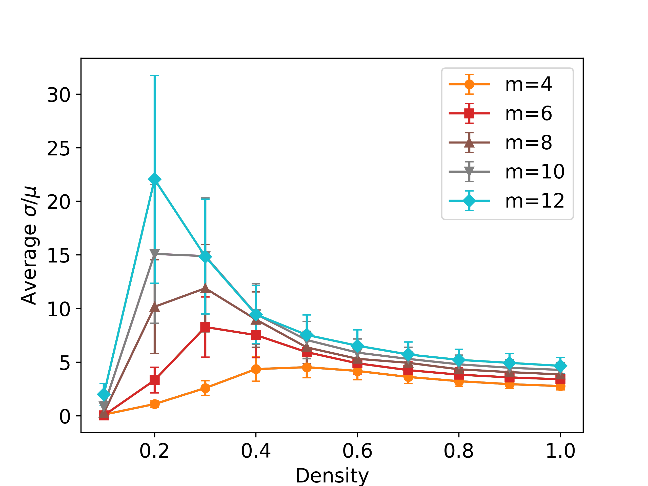
(b)

Figure 1: Average relative standard deviation $\sigma/\mu$ of (a) Godsil-Gutman and (b) Barvinok estimators for random graphs. Error bars denote confidence interval of one sigma, evaluated by bootstrap resampling and averaged over the sampled graphs.

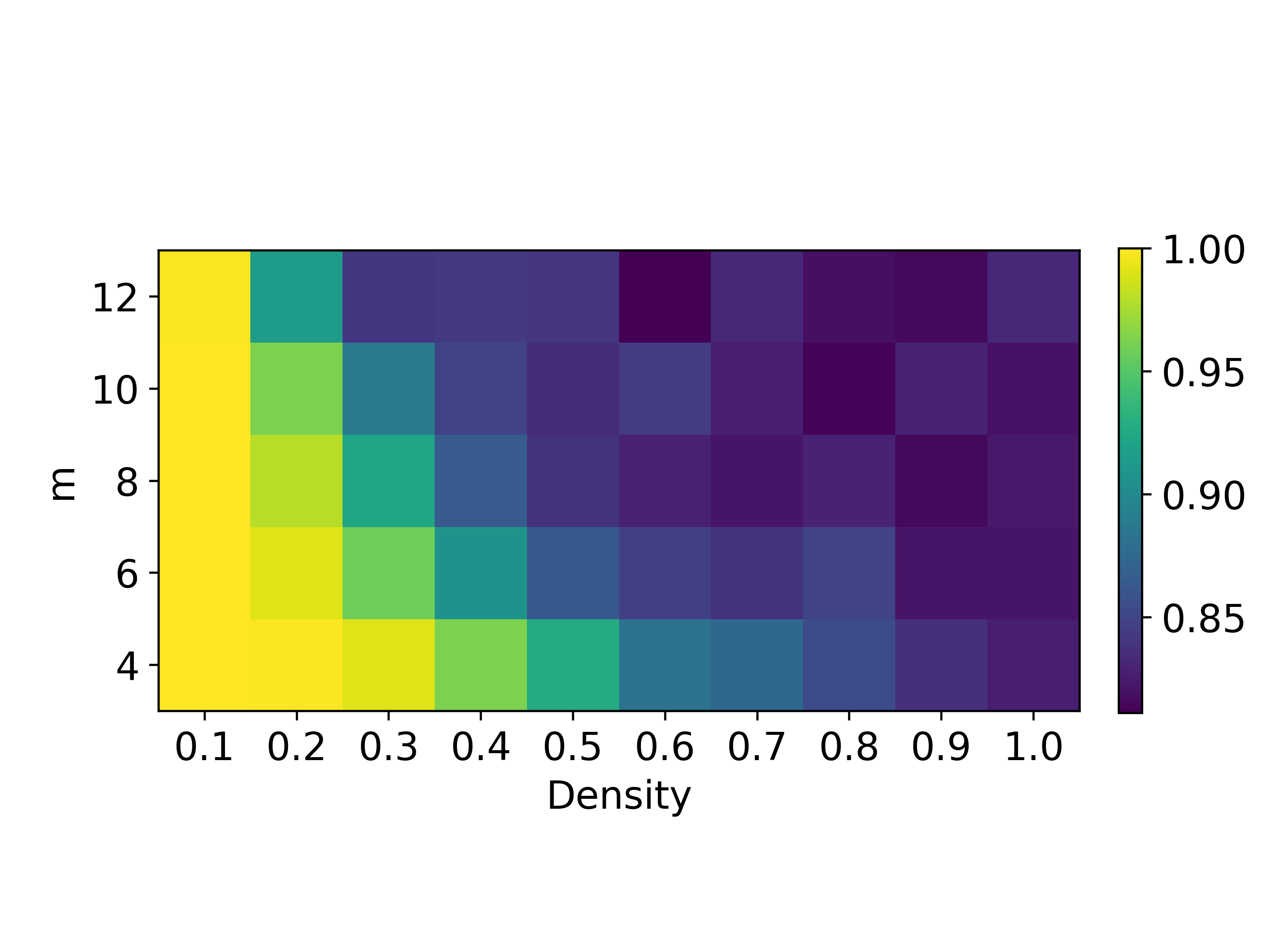
(a)

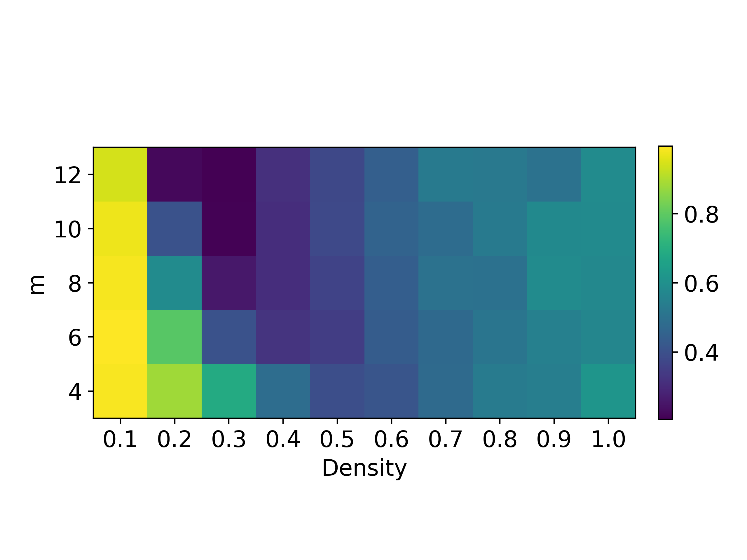
(b)

Figure 2: Share of graph instances with Hafnian calculated up to relative error $0.05$ using (a) Godsil-Gutman and (b) Barvinok estimators.

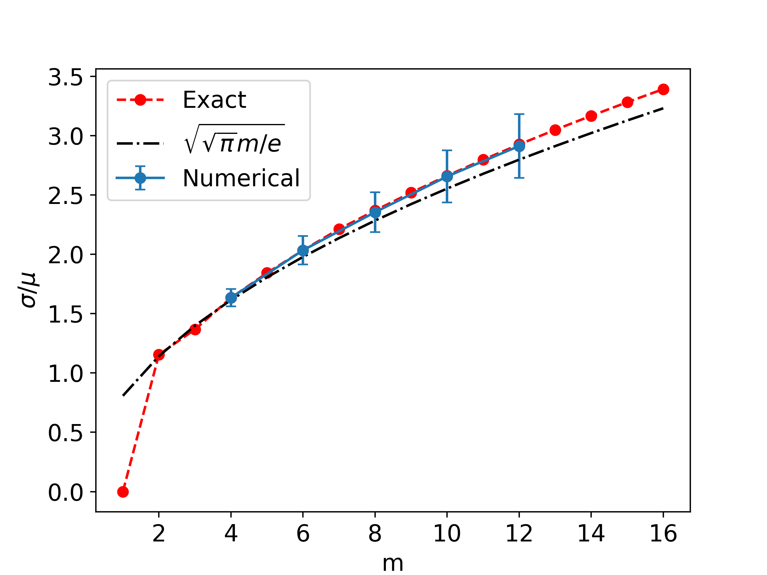
(a)

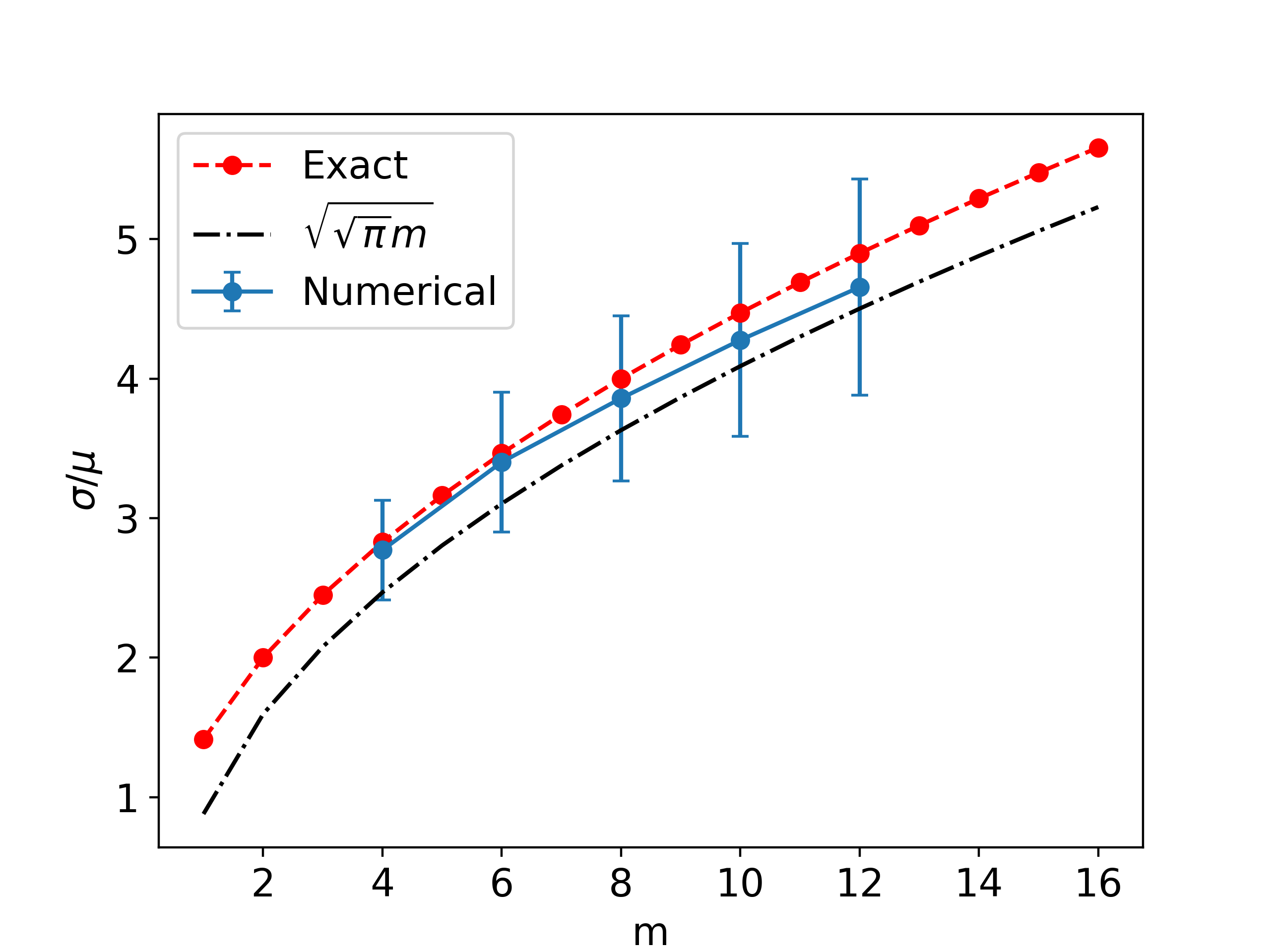
(b)

Figure 3: Relative standard deviation $\sigma/\mu$ of (a) Godsil-Gutman and (b) Barvinok estimators for the complete graphs of different sizes. The dashed line shows the exact values computed using the Taylor expansion of (15), the dash-dotted line shows the asymptote (20).

Knowing the generating function, we can conduct the analysis of asymptotic behavior of its series expansion using the Darboux’s method [18, 19]. First, define $\alpha=(t-3)/2$ and $y=x^{2}$. Define $g(y)=f(x)$:

$$g(y)=\frac{e^{\alpha y}}{(1-y)^{3/2}}.$$ (16)

Expanding the numerator around $y=1$, we obtain the following:

$$g(y)=e^{\alpha}\left((1-y)^{-3/2}-\alpha(1-y)^{-1/2}\right.+\\ \left.+\frac{\alpha^{2}}{2}\sqrt{1-y}+R(y)\right).$$ (17)

Here $R(y)$ contains all the remaining terms of the Taylor expansion and is once continuously differentiable at $|y|=1$. The $n$-th term in the series expansion of $g(y)$ is then equal to

$$[y^{n}]g(y)=e^{\alpha}\left(\binom{n+1/2}{n}-\alpha\binom{n-1/2}{n}+\right.\\ \left.+\frac{\alpha^{2}}{2}\binom{n-3/2}{n}+o\left(\frac{1}{n}\right)\right).$$ (18)

Here the last term of the expansion is vanishing faster than $1/n$ due to the Darboux’s theorem. Expanding the binomial coefficients and using the Striling’s formula for the gamma function, we obtain:

$$[y^{n}]g(y)=\frac{2}{\sqrt{\pi}}e^{\alpha}\sqrt{n}+O\left(\sqrt{\frac{1}{n}}\right).$$ (19)

This means that the expected square of the determinant (3) for a complete graph on $2m$ vertices tends to $\frac{2}{\sqrt{\pi}}e^{\alpha}\sqrt{m}(2m)!$ as $m$ goes to infinity. To calculate the relative variance, we recall that the number of perfect matchings in a complete graph is equal to $(2m-1)!!$. Gathering all the terms and using once again the Stirling’s formula for the factorials, we obtain:

$$\frac{\mathbb{E}\det G^{2}}{(\operatorname{Haf}A)^{2}}=\frac{(2m)!(\frac{2}{\sqrt{\pi}}e^{\alpha}\sqrt{m}+O(1/\sqrt{m}))}{((2m-1)!!)^{2}}=\\ =\sqrt{\pi}me^{\alpha}+O(1).$$ (20)

Thus, the relative error of either estimator grows as $\frac{\sqrt{m}}{\sqrt{N}}$, which implies that the number of samples $N$ should grow linearly with the size of the graph to preserve the same relative tolerance. Surprisingly enough, the fourth moment $\eta$ only changes the constant prefactor and not the overall scaling.

IV Relative error for random graphs

In this section, we investigate the behavior of Godsil-Gutman and Barvinok estimators for adjacency matrices of random graphs (that is, $a_{ij}\in\{0,1\}$). We sample graphs from the Erdös-Rényi ensemble $G_{2m,p}$ for different values of $p$ and $m$. For each graph, we take $N=500\cdot m$ samples of the estimator and compute their sample mean and sample variance. We also compute the exact Hafnian of the graph. Using this data, we evaluate the relative standard deviation $\sigma/\mu$. Here, the choice of sample size $N$ is informed by the results of the previous section, implying that under this scaling of sample size, the complete graph should demonstrate an asymptotically constant relative error. Finally, we estimate the accuracy of determining $\sigma/\mu$ by bootstrap resampling ($n=100$).

Fig. 1 shows the behavior of $\sigma/\mu$ for both estimators. The average $\sigma/\mu$ for the Godsil-Gutman estimator (Fig. 1a) exhibits a monotonous growith with $p$ for all values of $m$ considered. Interestingly, the error first grows with $p$ quite sharply, then flattens out and becomes relatively constant. The width of the growth period and its location both change with the increase of system size, shrinking and moving towards smaller values of $p$. The average error for the Barvinok estimator (Fig. 1b) demonstrates a substantially more complicated behavior. Instead of being monotonous with the density, the error shows a distinct peak. The location of the peak appears to match the location of the sharp growth region for the Godsil-Gutman estimator.

The sample variance alone might not contain the whole information about the estimate. For example, the disjoint graph discussed in Sec. II generates a distribution of determinants which has a high probability of observing zero and an extremely small probability of observing a very large value. In this case, a sample of all zeros would show zero relative sigma, which would be far from true. To account for that, we also studied the relative error of the estimator $|\bar{\mu}-\operatorname{Haf}A|/\operatorname{Haf}A$. Fig. 2 shows the share of graph instances for which the relative error is smaller than $0.05$. While there is some threshold behavior closely resembling that in Fig. 1, overall there does not seem to be any situation where the Godsil-Gutman estimator would dramatically fail to estimate the Hafnian. Notably, for higher densities, the success rate appears to be constant with respect to $m$, confirming the results of Section III.

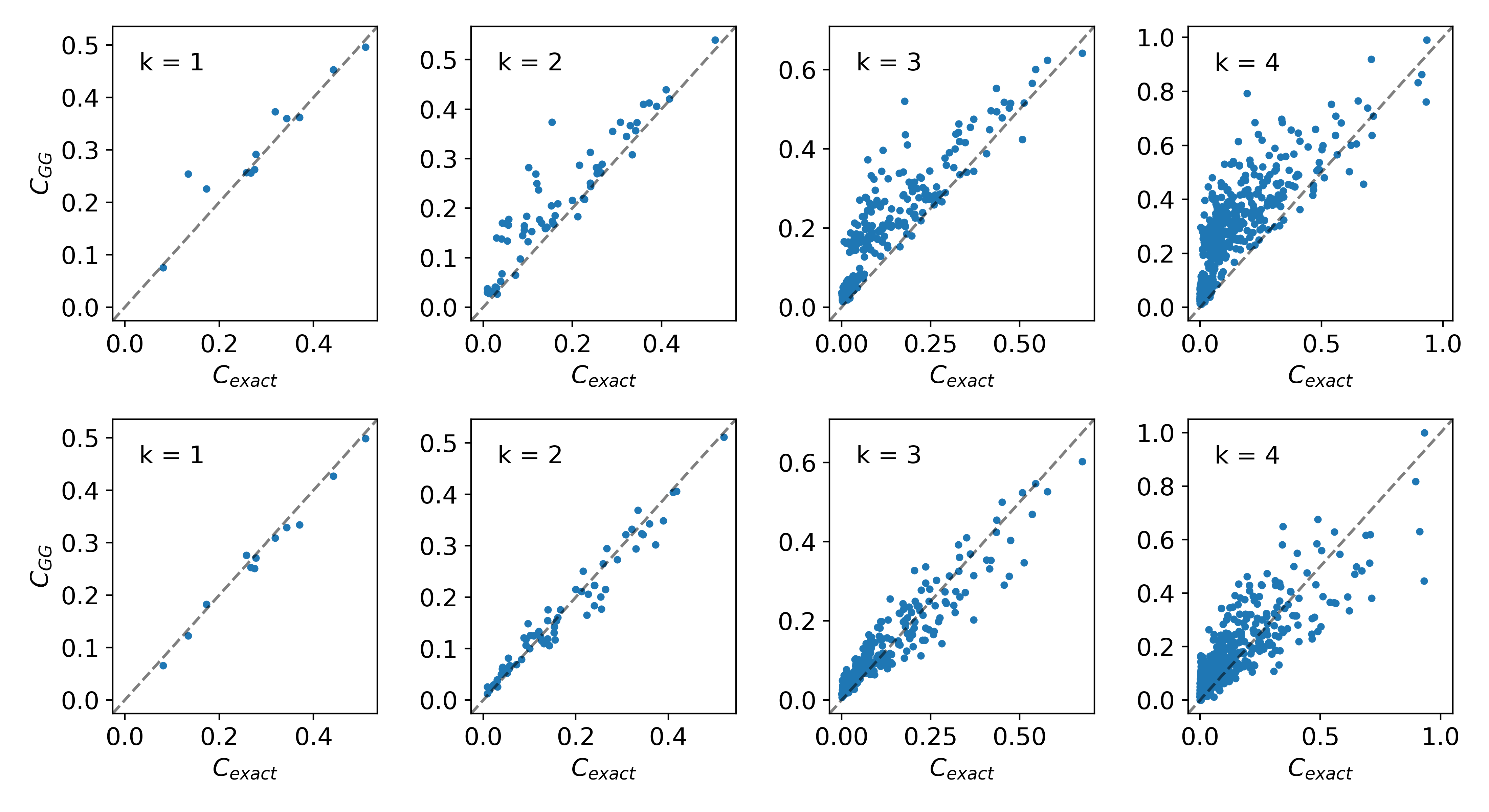
Figure 4: Correlation functions for the GBS experiment obtained with Godsil-Gutman sampling versus those obtained with exact sampling. Top row: $N=10$, bottom row: $N=1000$.

Finally, we compared the sampling data for $p=1$, all of which correspond to the complete graphs of different sizes, to the analytical estimates of Section III. As shown in Fig. 3, the estimated values of $\sigma/\mu$ show remarkable agreement with the theory. The asymptote $\sqrt{\sqrt{\pi}me^{\alpha}}$ also closely follows the exact values.

V Classical simulation of nonnegative GBS

We now turn to testing the approximate Hafnian estimation within the GBS setting, which we briefly recall here. A lossless GBS experiment for an $m$-mode Gaussian state with zero means is fully specified by a symmetric $2m\times 2m$ matrix $\mathcal{A}$ with singular values $\sigma_{i}\in[0,1)$, called the kernel matrix. Generally, the kernel matrix is complex, but here we restrict our attention to real and nonnegative matrices.

We consider the case of photon number resolving detectors, meaning that the detector can distinguish how many photons have arrived, as opposed to threshold detectors which can only tell whether any photons are present. The probability to observe an outcome $\mathbf{n}=(n_{1},n_{2},...,n_{m})$ is then equal to

$$P(\mathbf{n})=\frac{1}{n_{1}!\dots n_{m}!\sqrt{\det Q}}\operatorname{Haf}(\mathcal{A}_{\mathbf{n}}).$$ (21)

Here $Q$ is the covariance matrix, expressed from $\mathcal{A}$ as follows:

$$Q=\left(I-\begin{pmatrix}0&I\\ I&0\end{pmatrix}\mathcal{A}\right)^{-1}.$$ (22)

The matrix $\mathcal{A}_{\mathbf{n}}$ is obtained from $\mathcal{A}$ in two steps. First, one constructs an intermediate matrix by taking the first column of $\mathcal{A}$ for $n_{1}$ times, the second column $n_{2}$ times, and so on until the $m$’th column, after which one repeats the column $i+m$ for $n_{i}$ times. Then, the matrix $\mathcal{A}_{\mathbf{n}}$ is constructed from the intermediate matrix by repeating the same procedure with the rows.

When the state is pure, the kernel matrix $\mathcal{A}$ is simplified to $\mathcal{A}=A\oplus A^{*}$. In this case, $A$ is also referred to as a kernel matrix. The kernel matrix of a pure state is connected to the squeezing values $r_{i}$ and the interferometer unitary $U$ by the Autonne-Takagi decomposition:

$$A=U\operatorname{diag}(\tanh{r_{1}}\ \dots\ \tanh{r_{m}})U^{T}.$$ (23)

The proposed graph-related applications of GBS work by setting $A$ to be equal to the adjacency matrix of the problem graph, up to appropriate scaling.

We simulated GBS for a kernel corresponding to the adjacency matrix of an Erdös-Rényi graph with $m=12$ and $p=0.5$. We produced 1000 samples using the conditional probability method described in Ref. [11], using the Godsil-Gutman estimator of the Hafnian ($N=10$ and $N=1000$ determinants per Hafnian estimation), as well as the exact Hafnian calculation. We capped the maximum number of photons per mode at $n_{max}=4$. The kernel matrix was normalized so that the expected number of photons at $n_{max}=\infty$ would be equal to $\sqrt{m}$.

To compare the obtained samples, we studied the correlation functions $C(i_{1},...,i_{k})=\langle n_{i_{1}}...n_{i_{k}}\rangle$ for $k\in\{1,2,3,4\}$. We denote the correlations $C_{GG}$ when they are obtained from Godsil-Gutman sampling and $C_{exact}$ when they are obtained from exact sampling. The results are shown in Fig. 4. The samples obtained with $N=10$ demonstrate a noticeable deviation from their exact counterparts, while those obtained with $N=1000$ show good agreement with the exact sampling data.

VI Conclusions

In this manuscript, we analyzed the behavior the Godsil-Gutman and Barvinok estimators of the Hafnian of a real nonnegative matrix. Despite the existence of particular examples where one needs an exponential number of samples to achieve a constant relative error, the overall performance of both methods for random graphs was surprisingly good. This shows that the usage of GBS for the densest $k$-subgraph problem is unlikely to provide an exponential speedup except possibly for some particular family of graphs.

The simulability of Boson Sampling in certain regimes has been extensively studied in the literature. Specifically, there is a substantial body of work dedicated to the simulation of Boson Sampling in the imperfect conditions. In particular, it was found that Fock Boson Sampling with partially distinguishable photons [20], as well as FBS with sufficient photon loss [21], can be simulated classically in polynomial time. There are approximate classical sampling algorithms for noisy GBS as well [22, 23]. However, numerical experiments show that a noisy boson sampler is not much worse than a noiseless one when it is used to solve the $k$-densest subgraph problem [24]. Together with the efficient simulability of noisy GBS, this hints that the advantage derived from a quantum device is at best polynomial. In addition, Ref. [25] proposes a quantum-inspired classical algorithm for the $k$-densest subgraph problem and shows that the performance is also comparable to quantum sampling.

In conclusion, our work, together with the evidence from the existing literature, suggests (though does not yet decisively prove) that the ability to perform GBS with a nonnegative kernel does not provide quantum advantage. We suspect that there is a method to deal with the special cases where the Godsil-Gutman estimator fails, and that by finding it one can construct a fully polynomial randomized approximation scheme (FPRAS) for the Hafnian of a nonnegative matrix.