Fluctuation-Dissipation relations from a modern perspective

Abstract

In this review, we scrutinize historical and modern results on the linear response of dynamic systems to external perturbations and the celebrated relationship between fluctuations and dissipation expressed by the Fluctuation-Dissipation Theorem (FDT). The conceptual derivation of FDT originated from the definition of the equilibrium state and Onsager’s regression hypothesis. Over the time the fluctuation-dissipation relation was vividly investigated also for systems away from equilibrium, frequently exhibiting wild fluctuations of measured parameters. In the review, we recall the major formulations of the FDT, such as those proposed by Langevin, Onsager and Kubo. We discuss as well the importance of fluctuations in a wide class of growth phenomena. We point out possible generalizations of the FDT formalism along with a discussion of situations where the relation breaks down and can be not adapted.

I Introduction

Most physical observables accessible to experimental measurements comprise many components: particles or atoms. It turns out that in order to understand the outcome of the measurement experiments and claim its predictability, it is neither possible nor reasonable to follow the motion of all these constituents. Instead, one is using the concept of deviations from the expected outcome. Similarly, erratic motion of pollen in water suspension is the outcome of many collisions with the solvent molecules Brown28 ; Brown28a . The jiggling (the zigzag displacement) of observed pollen molecules and abrupt changes of velocities in course of their motion result from those collisions powered by thermal noise Langevin08 ; Nyquist28 ; Johnson28 ; Onsager31 ; Callen51 ; Callen52 . This is thermal noise that forces the motion and causes observable disturbances of trajectories; the same source of fluctuations supplies energy to molecular motorsJulicher97 ; Astumian94 ; Schliwa03 ; Baroncini19 ; Chowdhury13 ; Astumian96 ; Hoffmann16 ; Bao03 ; Bao06 ; Nettesheim20 , empowers chemical reactive paths Conca04 and can amplify the signal in the phenomenon of stochastic resonance Gammaitoni98 ; Benzi81 , and growth Barabasi95 ; Edwards82 ; Kardar86 . Implications of fluctuations are crucial in many areas of natural sciences, ranging from microscopic systems and molecular biology to ecology, models of financial markets Gontis10 , analysis of social contacts Urry04 and climate dynamics Chekroun11 . In Figure 1 we show some well-known phenomena where fluctuations play a fundamental role, such as diffusion (on the left) and growth phenomenon (on the right).

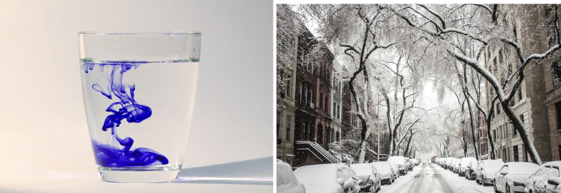
Figure 1: The images from left to right present some effects of fluctuations: a classical problem of diffusion of an ink drop in water figure1 and a random snowfall on cars, street and trees represents deposition pattern, which is fundamental in growth dynamics figure2 .

The aim of this work is to review some historical and recent works concerning the linear response theory associated with fluctuations, i.e., the several forms of the Fluctuation-Dissipation theorem (FDT), being organized as follows: We start by scrutinizing briefly the concept of fluctuations around equilibrium. In the next step we pass to the Langevin formalism and the FDT, while discussing the mechanism driving a system to equilibrium. In Section I.3, the Langevin’s heritage is presented, calling readers’ attention to some classical references. Section II is devoted to the growth mechanisms and the most challenging form of Langevin’s growth equation Barabasi95 ; Edwards82 ; Kardar86 is presented along with the discussion of the Kadar-Parisi-Zhang formalism Kardar86 . The Kubo approach towards FDT Kubo91 and some modern applications of it are recalled in Section III. In Section IV we discuss limitations of the fluctuation-dissipation formalism and some basic theorems associated with it. The ongoing research in the field and conclusions are drawn in Section V.

I.1 Fluctuations around equilibrium

The major results from Gauss’s work on observation errors and problem of statistical estimation in calculation of planetary orbits Gauss was to derive, based on the principle of least squares, the distribution of independent deviations from the most probable value of a measured quantity $x$

$$P(x)=\frac{1}{\sqrt{2\pi\sigma_{x}^{2}}}\exp{\left[-\frac{\left(x-\left\langle x\right\rangle\right)^{2}}{2\sigma_{x}^{2}}\right]}.$$ (1)

Here $\left\langle x\right\rangle=\frac{1}{N}\sum_{i=1}^{N}x_{i}$ denoted the arithmetic mean of observed values and $\sigma_{x}^{2}=\left\langle x^{2}\right\rangle-\left\langle x\right\rangle^{2}$ was interpreted as the precision or the dispersion in a set of measures.

About the same time, Laplace Laplace successfully accounted for all the observed deviations of the planets from their theoretical orbits by applying Sir Isaac Newton’s theory of gravitation and developed a conceptual view of evolutionary change in the structure of the solar system. Alike Gauss, he demonstrated the usefulness of a probabilistic approach for interpreting scientific data and systematized what is now known as probability theory, where the distribution, Eq. (1), plays a fundamental role in the description of an average outcome of a large number of statistically independent measurements and signals frequency of deviations (fluctuations) around the mean.

Fluctuation phenomena play a crucial role in thermodynamics, especially in nano-meter scale systems, where they are responsible for a large variability of functional properties. Thermodynamic systems at equilibrium are characterized by fluctuations that manifest the inherent discreteness of their microscopic states. At the dawn of kinetic theory, the empirical laws of an ideal gas were the first challenges to be understood and explained in terms of the theory of fluctuations. The probability of finding a molecule in the gas with a velocity between $v$ and $v+dv$ was then associated with the distribution, Eq. (1). This proposal worked well for a gas at high temperature and low density (non-interacting ideal gas), and it was confirmed experimentally. Moreover, by considering that the total energy is only the kinetic energy, it was possible to determine the velocity dispersion in each direction $x,y$ and $z$ separately, $\sigma_{v_{x}^{2}}=\sigma_{v_{y}^{2}}=\sigma_{v_{z}^{2}}=\left\langle v_{x}^{2}\right\rangle=\frac{RT}{M}$, where $M$ is the molecular mass of the particle, $T$ the absolute temperature and $R$ the universal gas constant. Following this line of reasoning and using the Boltzmann-Gibbs postulate relating the number of accessible microscopic states $W$ to the entropy $S$ of an isolated system, $S\propto\log W$, it was possible to determine theoretically the average energy, specific heat and the law of the ideal gas. It could be also proved that Eq. (1) was the only distribution compatible with the conservation of momentum and energy.

From the first law of thermodynamics, an infinitesimal change in the internal energy $U$ of a system can be written as

$$dU=TdS-PdV+\mu dN,$$ (2)

where the thermodynamics quantities are: $T$ the temperature, $S$ the entropy, $P$ the pressure, $\mu$ the chemical potential, and $N$ the number of particles inside the volume $V$. In the evolution of all quantities, one considers that the entropy of an isolated system takes its maximum value at equilibrium, so that the fluctuations of thermodynamic variables away from this state must cause entropy to decrease. By considering Boltzmann-Gibbs definition of entropy, these fluctuations may be derived by expanding deviations of the entropy in quadratic approximation and invoking stability of the equilibrium state. Such an expansion leads to distribution Eq. (1), around mean, equilibrium values of parameters defining the state of the system Salinas01 ; Huang87 and some standard deviations can be easily determined, e.g.:

$$\sigma_{U}^{2}=k_{B}T^{2}Nc_{v},$$ (3)

where $k_{B}=R/N_{a}$ is the Boltzmann constant, with $N_{a}$ as the Avogadro’s number and $c_{v}=\frac{1}{N}(\frac{\partial U}{\partial T})_{V}$ is the specific heat at constant volume. Similarly, the deviations in the volume are related to the isothermal compressibility:

$$\sigma_{V}^{2}=k_{B}T\left\langle V\right\rangle\kappa_{T},$$ (4)

where the isothermal compressibility, $\kappa_{T}$, is given by:

$$\kappa_{T}=-\frac{1}{V}\left(\frac{\partial V}{\partial P}\right)_{T}.$$ (5)

For the magnetization $\mu$, close to a phase transition, $T\rightarrow T_{c}$, one readily obtains Falk69

$$\sigma_{\mathbf{\mu}}^{2}=k_{B}T_{c}\chi,$$ (6)

where $\chi$ stands for the susceptibility, $\chi=\partial\mathbf{\mu}/\partial h_{0}$, which means the derivative of the ensemble average of the magnetization $\mathbf{\mu}$ regarding the external magnetic field $h_{0}$. A similar relation was recently obtained for the order parameter $r$ of a noise-induced phase synchronization in a Kuramoto model Pinto16 ; Pinto17

$$\sigma_{r}^{2}=k_{B}T_{c}\chi,$$ (7)

after rephrasing analysis of entropy in terms of the stationary probability distribution derived from the Langevin description of the system. Above relations show that the responses $c_{V}$, $\kappa_{T}$, and $\chi$ are positive and associated with fluctuations. For an extensive physical system which is described by a state variable $x$, such that $\left\langle x\right\rangle\propto N\neq 0$, with $N$ representing the number of additive subunits contributing to $x$, the standard deviation or relative fluctuation of $x$ is given by

$$\frac{\sigma_{x}}{\left\langle x\right\rangle}\approx\frac{1}{\sqrt{N}}.$$ (8)

The last relation is known as the law of large numbers, which ensures that for large systems the fluctuations are small, but not negligible as seen in Eqs. (3-7). This is in agreement with our intuitive notion that the volume of a solid is a well-defined quantity. However, we know that close to a phase transition, such as solid-liquid, the volume of a sample of ice undergoes a brutal variation of $10\%$ of its original value. Such large fluctuations are in disagreement with Eq. (8), which supposes a Gaussian distribution in its derivation. They are in a perfect accordance with Eqs. (3) and (4), where we can see a divergence in $c_{V}$ and $\kappa_{T}$. Some mean field theories, such as the Van der Waals equation, exhibit an unstable region where $\kappa_{T}<0$. Fluctuations are the basis of statistical mechanics and large fluctuations are the fundamental concept for understanding phase transition. The properties of Gaussian statistics are well described in many textbooks, see e.g. Salinas01 ; Huang87 ; Paul13 .

I.2 Fluctuations out of equilibrium

The analysis of systems out of equilibrium is clearly more complicated, however, at the same time more rich and plenty of new phenomena, e.g diffusion, can be observed. The diffusion process is the simplest and general fluctuation mechanism in out of equilibrium systems. This dynamical mechanism transport particles, energy or even information towards equilibrium Morgado02 ; Costa03 ; Metzler99 ; Sancho04 ; Lapas07 ; Lapas08 ; Weron10 ; Thiel13 ; Dorea06 ; Mckinley18 ; Flekkoy17 . This transport occurs when the system is not homogeneous. The inhomogeneous medium gives origin to gradients which drives the system towards equilibrium situation.

For two centuries Brown28 ; Brown28a ; Vainstein06 ; Santos19 ; Metzler00 ; Metzler04 , the diffusion mechanism has been intensively investigated because it plays an important role in many kinds of systems. The well-known experiments performed by Robert Brown drew attention to the stochastic trajectories of microscopic grains of pollen Brown28 which he associated, at the first moment, with life. Later, he also observed the same phenomenon in coal dust Brown28a . In this way, he discovered a new and intriguing phenomenon which is now called after him: the Brownian motion. Although the individual trajectories seem indescribable, their averages have important information. For example, if we follow the particle’s position as a function of time along the $x$-axis, we have the average displacement, $\left\langle x\right\rangle=0$, and its mean square:

$$\sigma_{x}^{2}=\left\langle\left(\Delta x(t)\right)^{2}\right\rangle,$$ (9)

where $\Delta x=x(t)-x(0)$ is the particle dislocation from the origin in a time $t$. For normal diffusion in one dimension,

$$\sigma_{x}^{2}=2Dt,$$ (10)

where $D$ is the diffusion constant. The above equation is known as the Einstein’s relation for diffusion Oliveira19 .

In the next section, we discuss the Langevin work on diffusion, where he introduced the first stochastic equation of motion for a particle and the first form of the FDT. As we shall see later, its generalization can be written in the form of Mori’s equation and the Kubo FDT.

I.3 The Langevin equation and the fluctuation-dissipation theorem

In the early 20th century, the atomic theory was still very controversial. For some researchers the unknown answers for many questions were an enormous problem, for others a great stimulus. Einstein’s and Smoluchowski’s works on the Brownian motion originate a great impact. Under different approaches, P. Langevin, A.D. Fokker, M. Planck and A. Kolmogorov studied the Brownian motion as a special class of a stochastic Markov process Langevin08 ; Vainstein06 ; Oliveira19 ; Einstein1905 ; Einstein56 ; Nowak17 .

Langevin started the era of explicit stochastic process in physics considering the equation of motion for a particle moving in a fluid as Langevin08 :

$$m\frac{dv(t)}{dt}=-m\gamma v(t)+f(t),$$ (11)

where $m$ and $\gamma$ are the mass of the particle and the friction, respectively. The ingenious and elegant proposal was to modulate the complex interactions between the particles, considering all interactions as two main forces. The first contribution represents a frictional force, $-m\gamma v$, where the characteristic time scale is $\tau=\gamma^{-1}$ while the second contribution comes from a stochastic force, $f(t)$, with time scale $\Delta t\ll\tau$, which is related with the random collisions between the particle and the fluid molecules.

It is important to mention that for a stochastic variable $g(t)$ the average in a time interval $\tau_{0}$ can be estimated as

$$\overline{g(t)}=\frac{1}{\tau_{0}}\int_{-\tau_{0}/2}^{\tau_{0}/2}g(t+s)ds.$$ (12)

and, thus, the Boltzmann’s ergodic hypothesis (BEH) establishes that for a system in equilibrium,

$$\overline{g(t)}=\langle g(t)\rangle,$$ (13)

which means that the time average is equal to the ensemble average. We interchange both definitions except in the situations where the BEH fails. The fluctuating force $f(t)$, in Eq. (11), obeys the following conditions:
$(i)$ the mean force due to the random collisions on the particle is zero

$$\langle f(t)\rangle=0,$$ (14)

$(ii)$ there is no correlation between the initial particle velocity and the random force

$$\langle f(t)v(0)\rangle=0$$ (15)

and $(iii)$ the fluctuating force at different times $t$ and $t^{\prime}$ are uncorrelated

$$\langle f(t)f(t^{\prime})\rangle=B\delta(t-t^{\prime}),$$ (16)

being $B$ a constant to be determined. The above equation is known as a Gaussian process or also called as white noise. In order to understand the dynamical properties of a particle that obeys the equation of motion (11) and the conditions (14) to (16), we start with the following solution:

$$v(t)=v(0)+\int_{0}^{t}\exp[-\gamma(t-t^{\prime})]f(t^{\prime})dt^{\prime}.$$ (17)

After a long time the system reaches the equilibrium, which means that

$$\langle v^{2}(t\rightarrow\infty)\rangle=\langle v^{2}\rangle_{eq}=k_{B}T/m.$$ (18)

(i.e. the equipartition theorem). We then use the above conditions to get $B=2m\gamma k_{B}T$ and rewrite Eq. (16) as

$$\langle f(t)f(t^{\prime})\rangle=2m\gamma k_{B}T\delta(t-t^{\prime}).$$ (19)

It was an ingenious idea of Langevin to separate the very complicated interaction of the molecules in the limiting time scale, i.e. the slow time change (the dissipative force) and the fast time change (the stochastic force ). It is noteworthy that this artificial separation between them in Eq. (8) now disappears as consequence of Eq. (19), where this important relation was pointed out between them. This was the first explicit form of the fluctuation-dissipation theorem (FDT).

Note that the Eqs. (3-7) establish a relation between a fluctuation and a response that can be easily measured. However, we now have an equation from which we can compute many response functions and treat systems which are not in equilibrium, but not so far from equilibrium. The first step is obviously to return to the diffusion problem. The mean square displacement can be written as:

$$\left\langle\left(\Delta x(t)\right)^{2}\right\rangle=\int_{0}^{t}dt^{\prime}\int_{0}^{t}dt^{\prime\prime}\langle v(t^{\prime})v(t^{\prime\prime})\rangle.$$ (20)

Next, we shall define the velocity-velocity correlation function as

$$C_{v}(t)=\left\langle v(t+t^{\prime})v(t^{\prime})\right\rangle,$$ (21)

and, in order to obtain $C_{v}(t)$, we multiply Eq. (11) by the set of initial conditions $\left\{v(0)\right\}$ and then we take the average to obtain the following equation:

$$\frac{d}{dt}C_{v}(t)=-\gamma C_{v}(t),$$ (22)

which can be solved analytically, producing the solution

$$C_{v}(t)=\frac{k_{B}T}{m}\exp(-\gamma t).$$ (23)

Thus, by introducing Eq. (23) into Eq. (20), we obtain an equation like Eq. (10), so the diffusion coefficient can be given by

$$D=\frac{k_{B}T}{m\gamma},$$ (24)

which is the same result obtained by Einstein. One can note that the Kubo relation

$$D=\int_{0}^{\infty}C_{v}(t)dt,$$ (25)

was used in the previous step. Although we have performed our analysis for one-dimensional motion, the generalization of the equation (11) for $d$ dimensions can be obtained by just multiplying the result of Eq. (10) by $d$ Einstein1905 ; Einstein56 . Now we can take the time average to obtain

$$\overline{v(t)}=\langle v(0)\rangle R(t),$$ (26)

and

$$\overline{v^{2}(t)}=\langle v^{2}\rangle_{eq}+R(t)^{2}\left[\langle v^{2}(0)\rangle-\langle v^{2}\rangle_{eq}\right],$$ (27)

with

$$R(t)=\frac{C_{v}(t)}{C_{v}(0)}=\exp{(-\gamma t)},$$ (28)

where the subscript $eq$ stands for equilibrium. Note that as $t\rightarrow\infty$ the system reaches equilibrium, with a null average velocity (space isotropy).

At this point, it is important to mention that after theoretical works by Einstein, Langevin, and Smoluchowski numerous experimental evidence has been established confirming the theory of Brownian motion.

I.3.1 The fluctuation-dissipation driving to equilibrium

As exposed above, it is easy to see that Langevin’s mechanism drives the system to equilibrium. In this way, in this subsection we exhibit this result for a complex system and we discuss better this mechanism.

First, let us solve Eq. (11) for a system of $N$ particles, using $\tau=\gamma^{-1}$ and $\Delta t=0.005\tau$, the Brownian force $f(t)$ was then taken to be constant during each time increment and of magnitude $x\sqrt{6m\gamma k_{B}T/\Delta t}$, with random numbers $x$ distributed uniformly in the interval $-1\leq x\leq 1$ and $T$ representing the reservoir temperature. The initial conditions for the numerical integration were that of uncorrelated non-Gaussian distribution of velocities in the form $v(0)=\pm\sqrt{k_{B}T_{0}/m}$. Figure (2) displays the instantaneous kinetic energy average per particle, $A(t)=\left\langle\frac{1}{2}mv^{2}(t)\right\rangle$, as a function of time of a typical simulation Vainstein06 . Energies are given in units of $k_{B}T$ and the time in units of $\tau$. The floating lines are plotted for $N=500$ particles and they exhibit large fluctuations, while the continuous ones are shown for the ensemble of $N=10^{6}$ particles. In this scale there is no visible difference between the exact results Eq. (27) and the simulations for $N=10^{6}$ particles. By setting the initial temperature $T_{0}$ for each independent system, (a) $T_{0}=T$ and (b) $T_{0}=3T$, one observes that both the curves plateau after the thermal equilibrium. Thus, the fluctuations are as that expressed by Eqs. (3) and (8).

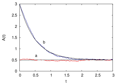
Figure 2: The evolution of the instantaneous average kinetic energy $A(t)$ as function of $t$ for various temperatures: (a) $T_{0}=T$; (b) $T_{0}=3T$. Reproduced from reference Vainstein06 with permission from Springer Lecture Notes in Physics.

In the above example, neither the initial conditions for the velocities nor the noise were Gaussian. It would make a lot of people scream. However, it is not really necessary. At the end of the day, the final set of velocities reaches a Gaussian distribution. The question is, how about the noise? We try to answer that question below.

For a system of interacting particles we just have to add the interacting force into Eq. (11). Let us consider, for example, a classical chain with $N$ monomers Oliveira94 ; Oliveira95 ; Oliveira00 . The Langevin’s equation for a particle of mass $m$ in a site $i$, with $i=1,2,\cdots,N$, is

$$m\frac{d^{2}q_{i}}{dt^{2}}=-m\gamma\frac{dq_{i}}{dt}+F(a+q_{i}-q_{i-1})-F(a+q_{i+1}-q_{i})+f_{i}(t).$$ (29)

where $F$ is a force between the next neighbors, $a$ is equilibrium position, which means $F(a)=0$, $q_{i}$ the displacement from the equilibrium position and $f_{i}(t)$ is a random force. A simple process to renormalize the equation of motion is to do a decimalization Oliveira95 ; Oliveira00 , which consists in rewrite the equations of motions in order to eliminate the intermediate site. For example, if the interaction is between a site $i$ and its neighbors $i\pm 1$, we eliminate these sites to get an interaction between the site $i$ and its next neighbors $i\pm 2$. Thus, let us define $y_{i}=q_{i+1}-q_{i}$ and subtract two successive equations Eq. (29) to obtain

$$m\frac{d^{2}y_{i}}{dt^{2}}=-m\gamma\frac{dy_{i}}{dt}-F(a-y_{i-1})+2F(a+y_{i})-F(a-y_{i+1})+[f_{i+1}-f_{i}(t)].$$ (30)

Note that renormalization for the positions is simple if $F$ is linear Oliveira00 , $F(a+y)=-Cy$, with $C$ as a constant; for nonlinear forces it is much more complicated Oliveira95 . However, for the noise which is independent of the lattice, the renormalization is trivial. For simplicity let us consider the noise as discrete $f_{i}=\Lambda j$, with $j=\pm 1/2$, intensity $\Lambda$ and probability $W_{0}(j)=1/2$. In Eq. (30) $f_{i+1}-f_{i}$, or equivalently $f_{i+1}+f_{i}$, has now $j=0,\pm 1$ with probabilities $W_{1}(0)=1/2$ and $W_{1}(\pm 1)=1/4$. For a general iteration of order $n$ we have

$$W_{n}(j)=\sum_{l}W_{n-1}(l)W_{n-1}(j-l),$$ (31)

i.e. the sum of all $l$ and $j-l$ that gives a $j$. $W_{n}(j)$ is a binomial distribution Oliveira00 , such as the one obtained in the study of the unbiased drunk motion Salinas01 . However, it is quite interesting to get it from the equations of motion. As $n\rightarrow\infty$, $W_{n}(j)$ becomes a Gaussian as required by the central limit theorem (CLT).

If from the very beginning we consider the noise distribution as continuous, after $n$ iterations we get the convolution

$$P_{n}(x)=\int_{-L_{n-1}}^{L_{n-1}}P_{n-1}(y)P_{n-1}(x-y)dy,$$ (32)

here $L_{n}=2L_{n-1}$. For example, if we consider the random numbers $x$ distributed uniformly in the interval $-1\leq x\leq 1$, i.e $P_{0}(x)=1/2$, and $L_{0}=1$, we get from the convolution (32):

$$P_{1}(x)=\begin{cases}\frac{1}{4}\left(2-|x|\right),&\text{ for ~{}~{} }|x|\leq 2\\ 0,&\text{ for ~{}~{} }|x|>2,\end{cases}$$ (33)

and using Eq. (32) again we obtain

$$P_{2}(x)=\begin{cases}\left(32-12x^{2}+3|x|^{3}\right)/96,&\text{ for ~{}~{} }|x|\leq 2\\ \left(4-|x|\right)^{3}/96,&\text{ for ~{}~{} }2\leq|x|\leq 4,\\ 0,&\text{ otherwise. }\end{cases}$$ (34)

In Figure (3) we plot the density of probability $P_{n}(x)$ as a function of $x$ for $n=0,1,2$. Note that $P_{2}(x)$ is almost a Gaussian.

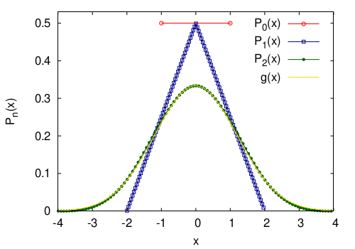
Figure 3: The density of probability $P_{n}(x)$ of getting a noise with intensity between $x$ and $x+dx$ as function of $x$. We start with the uniforme distribution $P_{0}(x)=1/2$. We plot $P_{n}(x)$, $n=0,1,2$, and the Gaussian $g(x)=\exp{-(\pi x^{2}/9)}/3$. We impose the Gaussian to have the same height as $P_{2}(x)$. From reference Oliveira95 with permission from PRB.

It is also interesting to note that if we apply the Fourier transform in Eq. (32), we get

$$\tilde{P}_{n}(k)=\tilde{P}_{n-1}(k)^{2},$$ (35)

which we can denote as the invariants of the renormalization group transformation (IRGT), the functions which keep their form under the transformations. Note that a possible set of IRGT are given by $\tilde{P}_{n}(k)=\exp(-(c_{n}k)^{\nu})$ the constant $c_{n}$ obeys the scaling $c_{n+1}=2^{1/\nu}c_{n}$. As $n\rightarrow\infty$, the IRGT with $0\leq\nu\leq 2$, yields the Lévy funcions Levy37

$$L(\nu,x)=\frac{1}{2\pi}\int e^{(ikx)}e^{-(c|k|)^{\nu}}dk.$$ (36)

For $\nu=1$ we have a Lorentzian and for $\nu=2$ we have a Gaussian curve. Thus, Eq. (32) as $n\rightarrow\infty$ and $P_{n}(x)=P(x)$ bring us to the generalized central limit theorem (GCLT). Note that, if we study for example the velocity as in Figure (2), one obtains $A(t\rightarrow\infty)=\frac{1}{2}k_{B}T$, i.e. a finite momenta. Since in the set of functions (36) the Gaussians are the only one with all the momenta finite, thus Gaussian distributions are the most expected outcome after equilibrium is reached. Note that Eq. (31) or Eq. (32) are independent of the forces $F$ between the neighbors, thus they are very general. The extraordinary success of Langevin’s way to nonequilibrium statistical mechanics gives us what we can call Langevin’s heritage, as we shall see further on.

The beautiful and simple Langevin approach helps us to deal with many situations in physics. It allows us to do some analytical calculations for some simplified models and even to get some limiting results for more complex systems. As well is easy to perform computer experiments within his framework. Therefore, the Langevin equation, and its quantum formulation (Sec. III), with the concept of fluctuating fields, opened a wide branch of investigations in many systems, such as light scattering Leite64 ; Penna76 ; Marcus60 ; Oliveira81 ; Loudon00 ; Santos00 ; Benmouna01 ; Oliveira81b , neutron scattering in liquids metals Rahman62 ; Yulmetyev03 , polymer chain dynamics Florencio85 ; Odell94 ; Toussaint04 ; Doerr94 ; Oliveira96 ; Oliveira98a ; Gonzalez99 ; Maroja01 ; Dias05 ; Sain06 ; Azevedo16 , molecular motors Bao03a ; Bao06 ; Qiu19 , conductivity Dyre00 ; Oliveira05 , reaction rate theory Kramers40 ; Oliveira98 ; Hanggi77 ; Hanggi90 , and noise synchronization Boccaletti02 ; Longa96 ; Maritan94 ; Ciesla01 ; Osipov07 ; Morgado07 . The use of diffusion concepts finds a plentiful of applications in science, for example, in controlled drug delivery, where the well-understanding of the drug release mechanisms as well as the characteristic release times is a must Siepmann12 ; GomesFilho16 ; Ignacio17 ; Singh19 ; mircioiu2019 ; GomesFilho20 ; Yang20 ; GomesFilho22 . All these phenomena, however, are some form of the wide, really wide field of anomalous diffusion Astumian94 ; Bao03 ; Morgado02 ; Sancho04 ; Lapas08 ; Weron10 ; Thiel13 ; Dorea06 ; Mckinley18 ; Santos19 ; Vainstein08 ; Mckinley18 ; Donato06 .

II Fluctuation and Growth

One of the most important manifestations in nature is the phenomenon of growth. It is ubiquitous in biology, where it occurs in process such as cell growth, population dynamics, and embryo development. It also plays a role in chemistry, where reagents and products exchange their populations, and in physics, where the stability of growth or lack thereof is often a question. Fluctuations are inherent in these processes, and we will discuss two basic types:

1. Small fluctuations, such as in populations dynamics

2. Large fluctuations, such as in material growth.

This choice covers a wide range of phenomena and are very active areas of research.

II.1 Small fluctuations and population dynamics

As stated above, the concepts of diffusion and fluctuations have found applications in many branches of natural sciences. The extension of these concepts has immediate application in the study of growth. Since growth phenomena are widely found in many dynamical processes in nature, they have received much attention in the dynamics study over the last years. In a rough classification, we can divide these studies into two types: one with small fluctuations where it appears as a perturbation, and a second one with large fluctuations. As an example of the first kind, let us consider the total population $N(t)$ in a given ecological niche. A simple equation to model this growth is given by

$$\dfrac{dN(t)}{dt}=aN(t)-bN(t)^{2},$$ (37)

where $a$ and $b$ standing for the growth and the competition rate, respectively. For $b=0$ we have the Malthusian exponential growth. The above equation is known as the logistic growth of Verhulst Banks94 ; Murray2002 , which imposes a limit for growth $N(t\rightarrow\infty)=a/b$. In a more elaborate analysis we want to know not only the total number $N(t)$, but the local density $u(\vec{x},t)$, which propagates in time and space, such as in the famous Fisher equation Fisher37

$$\frac{\partial u(x,t)}{\partial t}=au(x^{\prime},t)+D\frac{d^{2}u(x,t)}{dx^{2}}-bu(x,t)^{2},$$ (38)

where D is diffusion coefficient. Now $N(t)=\int u(\vec{x},t)d\vec{x}$. Note that the uniform density $u_{0}=a/b$ is as well a solution of the above equation. Fisher was the first to show that bacterial populations can propagate as a wave, now denominated Fisher waves. This and subsequent studies suggested that we can model the evolution of the density by reaction-diffusion equations Banks94 ; Murray2002 ; Rothe84 . Recently, a general reaction-diffusion equation has been proposed Aranda20-1 ; Aranda20-2 ; Aranda21

$$\dfrac{\partial u(\vec{x},t)}{\partial t}=\hat{M}u(x,t),$$ (39)

where $\hat{M}$ is an operator acting on $u(\vec{x},t)$. In this form, Eq. (39) is quite general and can describe a large number of different physical systems (or properties), such as the evolution of a density of particles Landau65 ; Cross93 , energy, or even alive beings as in a colony of bacteria Fisher37 ; Murray2002 ; Turing52 ; Kolmogorov37 .

For simple systems, in which the operator $\hat{M}$ is linear, analytical solutions are readily obtained. However, most realistic systems are described by a non-linear $\hat{M}$ (cf. Eqs. (37) and (38)) with the operator implicitly depending on $u$, $\hat{M}=\hat{M}(u)$; in those cases analytical solutions are cumbersome and not so easily obtained.

Now we show an example of a one-dimensional system in the range $0<x<L$, described by an equation that includes nonlocal growth and interaction terms involving long-range effects in the system. This equation takes the form DaCunha11 :

$$\frac{\partial u(x,t)}{\partial t}=a\displaystyle{\int_{0}^{L}}g_{\alpha}(x-x^{\prime})u(x^{\prime},t)dx^{\prime}-bu(x,t)\displaystyle{\int_{0}^{L}}g_{\beta}(x-x^{\prime})u(x^{\prime},t)dx^{\prime},$$ (40)

where $\alpha$ and $\beta$ are the growth and competition length parameters, respectively. A simple choice for the nonlocal kernel is

$$g_{\kappa}(x)=\left\{\begin{array}[]{lcl}\frac{1}{2\kappa},&|x|<\kappa,&\\ 0,&\text{otherwise}.&\\ \end{array}\right.$$ (43)

Despite all complexity, there are some general characteristics for these systems. For instance, three questions need to be answered. First is about the existence of an uniform solution $\hat{M}u_{0}=0$, i.e. the constant density $u_{0}=a/b$. Note that Eq. (40) fulfil it. The second one, is this uniform solution stable? In addition, what happens when fluctuations disturb it? Landau proposed a simple and general answer in his studies of plasma stability Landau65 ; Cross93 . For him the fluctuations were just some small initial input to be added to the uniform solution $u_{0}$ in the form

$$u(\vec{x},t)=u_{0}+\epsilon\exp{\left[\gamma(k)t\right]}\cos{\left(\vec{k}.\vec{x}\right)},$$ (44)

where $\epsilon\ll u_{0}$ is a perturbation which, for large $t$, can either grow or die out, depending on the value of $\gamma(k)$. We then solve Eq. (39) in first order in $\epsilon$ to obtain $\gamma(k)$, in a such way that:

$$\gamma(k) < 0,\quad\text{the system evolves to the homogeneous steady-state,}$$ (45)

$$\gamma(k) > 0,\quad\text{the system departures from the homogeneous state, appearing patterns.}$$

This approach has been widely used in nonlinear dynamics to study pattern formation Oliveira96 ; Gonzalez99 ; Aranda20-1 ; Aranda20-2 ; DaCunha11 ; Koch94 ; Nicolis95 ; Newell97 ; Rabinovich20 ; Fuentes03 ; Fuentes04 ; DaCunha09 ; Colombo12 ; Barbosa17 .

As an example, Fuentes et al. Fuentes04 used

$$\frac{\partial u(x,t)}{\partial t}=au(x^{\prime},t)+D\frac{d^{2}u(x,t)}{dx^{2}}-bu(x,t)\displaystyle{\int_{0}^{L}}g_{\beta}(x-x^{\prime})u(x^{\prime},t)dx^{\prime},$$ (46)

to obtain

$$\gamma(k^{\prime})=-a\left[\frac{\sin\left(k^{\prime}\eta\right)}{k^{\prime}\eta}+k^{\prime}\right],$$ (47)

with $k^{\prime}=k\sqrt{D/a}$, $\eta=\beta\sqrt{a/D}$. This is illustrated in Figure (4), being $\gamma(k^{\prime})$ as function of $k^{\prime}$ for three different values of $\eta$: $50,10$ and $2$. Here $\gamma$ is in units of $a$, and $k$ in units of $L^{-1}$. Fluctuations with vales of $k^{\prime}$ such that $\gamma(k^{\prime})>0$ will be amplified those with $\gamma(k^{\prime})<0$ will die out. We apply again the Landau’s approach, Eq. (44), into Eq. (40) to get:

$$\gamma(k)=a\left[\frac{\sin\left(k\alpha\right)}{k\alpha}-\frac{\sin\left(k\beta\right)}{k\beta}-1\right],$$ (48)

Note that in order to have $\gamma(k)>0$ we must have small values of $\alpha$ and $\sin\left(k\beta\right)<0$. From DaCunha11 .

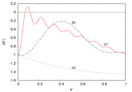
Figure 4: The effective growth rate $\gamma(k^{\prime})$ as function of $k^{\prime}$ for a small perturbation from the uniform density. (a) $\eta=2$; (b) $\eta=10$; (c) $\eta=50$. For values of $\gamma(k^{\prime})>0$, the system departures from the homogeneous state, appearing patterns. From Fuentes et al. Fuentes04 . With permission from JPC B.

At first glance, it may seem that Eq. (40) does not have a diffusive term. However, if we rewrite the first integral as DaCunha11 :

$$I(x)=a\displaystyle{\int_{0}^{L}}g_{\alpha}(x-x^{\prime})u(x^{\prime},t)dx^{\prime}=a\displaystyle{\int_{x}^{L+x}}g_{\alpha}(y)u(y+x,t)dy=a\sum_{n=0}^{\infty}\lambda_{n}\frac{d^{2n}u(x,t)}{dx^{2n}},$$ (49)

where we have used the Taylor expansion, the fact that $g_{\alpha}(x)$ is an even function, the periodic boundary condition $u(x+L,t)=u(x,t)$ and

$$\lambda_{n}=\frac{1}{(2n)!}\int_{0}^{L}g(y)y^{2n}dy.$$ (50)

Considering the first two terms in the expansion and $\beta\rightarrow 0$, we obtain the Fisher equation (38), with $D=\frac{1}{6}a\alpha^{2}$. This was used to obtain the values of $\alpha$, and to successfully describe the diffusion of Escherichia coli populations DaCunha11 . Consequently, in the expansion Eq. (49), the first term is the growth term, the second is the diffusive and the higher order terms, $n>1$, are the dispersive terms. Taking only the first two terms in the expansion and keeping the second integral we get the Fuentes at al. formulation Fuentes03 ; Fuentes04 . A considerable number of formulations may be regarded as a particular case of Eq. (40), see, for example, the Ref. Aranda20-2 .

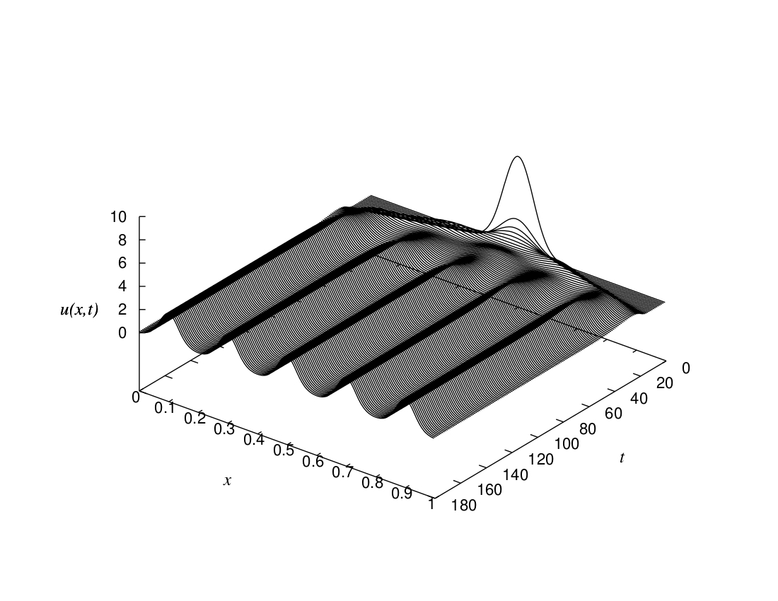
Figure 5: Typical time and space evolution of the density $u(x,t)$. It starts as a Gaussian and after a long time $u(x,t)$ converges to a steady state $u(x,t\rightarrow\infty)=U(x)$. From several authors Fuentes03 ; Fuentes04 ; DaCunha09 ; DaCunha11 .

In Figure (5) we show a typical curve of time and space evolution of the density $u(x,t)$. Here we use the values of Da Cunha al. DaCunha11 . $\alpha$, $\beta$, and $x$ are given in units of $x$, and $u$ in units of $L^{-1}$. The growth and interaction rates are $a=b=1$. In addition, the growth and competition length parameters are $\alpha=0.009$ and $\beta=0.15$, respectively. The results are from the solution of Eq. (40) by setting the initial distribution as a Gaussian centered at $x=L/2$. After a long time it evolves to a steady state solution $U(x)$, which means $u(x,t\rightarrow\infty)\rightarrow U(x)$. This type of evolution is found in many physical situations Fuentes03 ; Fuentes04 ; DaCunha09 ; DaCunha11 ; Aranda20-1 ; Aranda20-2 ; Aranda21 .

Finally, we define a very important quantity

$$\rho=\int_{0}^{L}[U(x)-u_{0}]dx,$$ (51)

i.e. considering $N_{0}=u_{0}L$ as the number of individuals that a system has with a uniform distribution, $\rho$ measures the deviation due to patterns formation, which means the breaking of translation symmetry creates a new order parameter.

Thus, we show in Figure (6) the parameter $\rho=\rho(\alpha,\beta)$ in the space $(\alpha,\beta)$, representing the quantity that exceeds the population for a uniform density $N_{0}=u_{0}L$. The results are from the solution of Eq. (40), being $\rho$ in units of $N_{0}$ just a number. Regions that exhibit patterns are those with $\rho>0$. Negative values of $\rho$ were not observed, i.e., $\rho\geq 0$, being the minimum value for the uniform distributions. This shows that one reason for nature to make patterns is that it allows more individuals to exist in a given ecological niche.

In the above formulations fluctuations are just a small perturbation which, may die, in this case $u(\vec{x},t\rightarrow\infty)=u_{0}$, or will grow up, driving the system towards a pattern, i.e. a non uniform density $u(\vec{x},t)$. We may include in population dynamics situations where the noise is strong  Fusco16 . However, we shall leave it for the next subsection, where we study growth phenomenon.

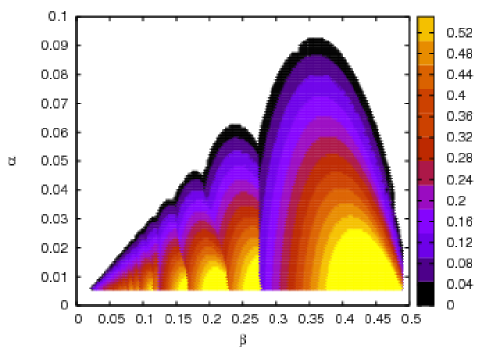
Figure 6: The phase diagram in the $(\alpha,\beta)$ space. The parameter $\rho>0$, colored column on the right, represents the extra population comported by the system due to patterns. From Barbosa et al. Barbosa17 . With permission from Physica A.

II.2 Non-perturbative fluctuations

Next, we will discuss a second kind of growth phenomenon that is very different from the previous one. Imagine a water reservoir of height $H$ and uniform lateral area. In order to establish how much water was deposited in the reservoir in time $t$, it is sufficient to measure time evolution of the height $h(t)$, $0<h(t)<H$. In most physical systems, the growth process occurs when particles, or aggregates of particles, reach a surface via diffusion or by injection, or in course of some kind of a deposition process of chemical or biological origin. For example, consider snow falling on the street as depicted in Figure 1. This is similar to the water being deposited in the reservoir, but now the interface is no longer uniform and each point of the surface may have a height $h(\vec{x},t)$, being $\vec{x}$ the position in the $d$ dimensional space and $t$ the time. In this way, the height $h(\vec{x},t)$ and the position $\vec{x}$ make a $d+1$ dimensional space. This form of growth where the interface is rough has been intensively investigated over the past four decades. Some more example are growth of semiconductors thin films Almeida14 , corrosion or etching mechanism Mello01 ; Gomes19 and fire propagation Merikoski03 , the last two are example of negative growth, i.e. $\langle\frac{\partial h(\vec{x},t)}{\partial t}\rangle<0$. In this way, there are many physical systems in nature that can exhibit one phase of growth, which makes it a prolific area of scientific research effort. In such systems fluctuations-driven stochastic dynamics leads to a rough interface which separates the two media Barabasi95 ; Edwards82 ; Kardar86 ; Hansen00 . Two quantities play an important rule in the growth dynamics, the average height, $\langle h(\vec{x},t)\rangle$, and the standard deviation

$$w(L,t)=\sigma_{h}=\left[\langle h(\vec{x},t)^{2}\rangle-\langle h(\vec{x},t)\rangle^{2}\right]^{1/2}.$$ (52)

The standard deviation provides us with a precise definition for the interface roughness. Thus, we name it roughness or the surface width. Here $\langle\cdots\rangle$ is the space average, and $L$ is the system size. It should be mentioned that the dispersion Eq. (52) is the main physical quantity to be obtained in the growth process, moreover, we would say that, in statistical physics, it is the second only to the diffusion, Eq. (9), and many important phenomena have been associated with it.

The general characteristics of the growth dynamics were observed through some analytical, experimental and computational results Barabasi95 . For many growth processes, the roughness $w(t)$ increases with time until it reaches a saturated roughness $w_{s}$, i.e., $w(t\rightarrow\infty)=w_{s}$. In Figure (7) we show the evolution of $w(t)$ as function of $t$ for a typical growth process. We can summarize the time evolution of all regions as following:

$$w(t,L)=\begin{cases}ct^{1/2},&\text{ if~{}~{} }t<<t_{0}\\ ct^{\beta},&\text{ if~{}~{} }t_{0}<<t_{\times}\\ w_{s}\propto L^{\alpha},&\text{ if~{}~{} }t>>t_{\times}.\\ \end{cases}$$ (53)

Here $t_{0}$ is a time before correlations start where we have pure diffusion, and $t_{\times}\propto L^{z}$. Note that the exponents $\alpha$ and $\beta$ here have no connection with the length parameters $\alpha$ and $\beta$ of the last section. Moreover, the dynamical exponents satisfy the general scaling relation:

$$z=\frac{\alpha}{\beta}.$$ (54)

Different methods have been proposed to understand this rich phenomenon. Here, we will be focused only on processes that saturate, i.e. these with a finite $w_{s}$, $w(t\rightarrow\infty)=w_{s}$. This occurs in a general class of growth phenomena. The attempt to describe the height evolution leads us to some equation of the form:

$$\dfrac{\partial h(\vec{x},t)}{\partial t}=\hat{G}h(\vec{x},t)+\xi(\vec{x},t),$$ (55)

where $\hat{G}$ is a deterministic operator and the stochastic process is characterized by the noise, $\xi(\vec{x},t)$, which in its simplest form is assumed Gaussian and white:

$$\left\langle\xi(\vec{x},t)\xi(\vec{x^{\prime}},t^{\prime})\right\rangle=2D\delta^{(d)}(\vec{x}-\vec{x^{\prime}})\delta(t-t^{\prime}),$$ (56)

with $D$ standing for the noise intensity.

The deterministic part of the RHS of Eq.(55) must obey certain symmetry rules Edwards82 such as time translation and height invariance. As well, $h\rightarrow-h$, and $\vec{x}\rightarrow-\vec{x}$. These symmetrical rules imply that only even-order of derivatives are allowed, which bring us to some form of Langevin equations. In the lowest order, the simplest field equation is Barabasi95 ; Edwards82

$$\dfrac{\partial h(\vec{x},t)}{\partial t}=\nu\nabla^{2}h(\vec{x},t)+\xi(\vec{x},t),$$ (57)

known as the Edwards-Wilkinson equation (EWE) Edwards82 , here the parameters $\nu$ is the surface tension, which tends to reduce the surface curvature. With this equation we can explain certain forms of growth, such as deposition with relaxation Barabasi95 . Note that if we exclude the noise, $D=0$, Eq. (57) becomes the diffusion equation discussed in the Introduction section. The presence of space-inhomogeneous and time dependent noise makes the process a more complicated form of diffusion. For $1+1$ dimensions, the exponents are $\alpha=1/2$, $\beta=1/4$, and $z=2$, in agreement with Eq. (54).

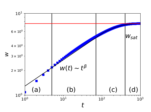
Figure 7: Time evolution of the roughness, $w(t)$, as a function of the time $t$ for the $1+1$ etching model. The sample has size $L=200$ and we take the time intervals as $\Delta t=1/L$, in such way that we reach on site on average for each unity of time. The growth process has different aspects in each region: (a) $0<t<t_{0}\approx 5$, where correlations have not yet started, the process is a random deposition $w(t)\sim t^{1/2}$; (b) when correlations starts to play a major rule $5<t<70$ the power law region $w(t)\sim t^{\beta}$; (c) the intermediate region $70<t<400$; (d) the saturation region $w(t)\approx w_{s}$, for $t>400$. From the figure we obtain the characteristic time $t_{\times}=167.0(2)$; that is, the saturation occurs for $t>>t_{\times}$ as exhibited in region (d). From Gomes et al. Gomes19 . With permission from PRE.

A large number of systems, however, cannot be described by the EWE. Consider for example the roughness evolution in Figure (7), obtained from the etching model Mello01 in $1+1$ dimensions. The etching model is described below. From that curve we obtain $\beta=0.330$, very far away from the Edwards Wilkinson results. Consequently, new forms of growth equations have been proposed. A new achievement was obtained when Kardar et al.  Kardar86 introduced a new term into EWE to obtain

$$\dfrac{\partial h(\vec{x},t)}{\partial t}=\nu\nabla^{2}h(\vec{x},t)+\dfrac{\lambda}{2}[\vec{\nabla}h(\vec{x},t)]^{2}+\xi(\vec{x},t),$$ (58)

where $\lambda$ is related to the tilt mechanism Kardar86 . The nonlinear term arises when we consider the lateral growth. Note that for $\nu=0$ we have the Burgers equation with noise. Now we have lost the symmetry $h\rightarrow-h$, and consequently we have a new universality class.

In order to summarize the basic information about KPZ, we shall add Kardar86 :

$$\alpha+z=2.$$ (59)

As a consequence of Galilean invariance in the related Burgers equation Forster97 .

II.2.1 Universality

In this way, the KPZ equation, Eq. (58), is a general nonlinear stochastic differential equation, which can characterize the growth dynamics of many different systems Mello01 ; Merikoski03 ; Odor10 ; Takeuchi13 ; Almeida17 ; Reis05 ; Almeida14 ; Rodrigues15 ; Alves16 ; Carrasco18 . Systems that exhibit the same exponents as KPZ belongs to the KPZ universality class. As consequence of that universality most of these stochastic systems are interconnected. For instance, the single step (SS) model Krug92 ; Krug97 ; Derrida98 ; Meakin86 ; Daryaei20 , which is connected with the asymmetric simple exclusion process Derrida98 , the six-vertex model Meakin86 ; Gwa92 ; Vega85 , and the kinetic Ising model Meakin86 ; Plischke87 , all of them are of fundamental importance. It is noteworthy that quantum versions of the KPZ equation have been recently reported that are connected with a Coulomb gas Corwin18 , a quantum entanglement growth dynamics with random time and space Nahum17 , as well as in infinite temperature spin-spin correlation in the isotropic quantum Heisenberg spin-$1/2$ model Ljubotina19 ; DeNardis19 , anisotropic quantum Heisenberg chain  Vainstein05 , and spin glass Prykarpatski23 .

In these processes, the randomness is not a small perturbation, it is a strong part of it, indeed $D$ is an important part of the theory. For example, the coupling parameter Kardar86

$$g=\frac{D\lambda^{2}}{\nu^{3}}$$ (60)

connects all KPZ parameters and it is a fundamental quantity for any renormalization process.

Despite all effort, finding an analytical, or even a numerical solution, of the KPZ equation (58) is not an easy task Dasgupta96 ; Dasgupta97 ; Torres18 ; Wio10a ; Wio17 ; Rodriguez19 and we are still far from a satisfactory theory for the KPZ equation, which makes it one of the most difficult and exciting problems in modern mathematical physics Bertine97 ; Baik99 ; Prahofer00 ; Dotsenko10 ; Calabrese10 ; Amir11 ; Sasamoto10 ; Doussal16 ; Hairer13 , and probably one of the most important problem in non equilibrium statistical physics. The outstanding works of Prähofer and Spohn Prahofer00 and Johansson Johansson00 opened the possibility of an exact solution for the distributions of the heights fluctuations $f(h,t)$ in the KPZ equation for $1+1$ dimensions  Calabrese10 ; Amir11 ; Sasamoto10 ; Doussal16 .

To define the fields of action in the investigation of KPZ dynamics, we have the main scenarios:

1. To describe experiments using KPZ dynamics;

2. To match a given model into KPZ;

3. Determination of the exponents and heights distribution;

4. To match a given KPZ model into another KPZ model.

We define as KPZ model, a model which belongs to the KPZ universality class. In our present stage of knowledge only in $1+1$ dimensions these questions have got precise answers.

II.3 Experiments described by the KPZ dynamics

We briefly present here some experiments well described by the KPZ approach. The first one is the more typical experiment of growth, where polycrystalline CdTe/Si(100) films grows by hot-wall epitaxy Almeida14 . In Figure (8) we show the evolution of morphology for different times of the growth. The roughness of the surface becomes clear. From that they obtained the exponent $z=1.61(5)$. Note that while the sample size are measure in $\mu m$ the roughness exposed in the $z$ axes are in $nm$.

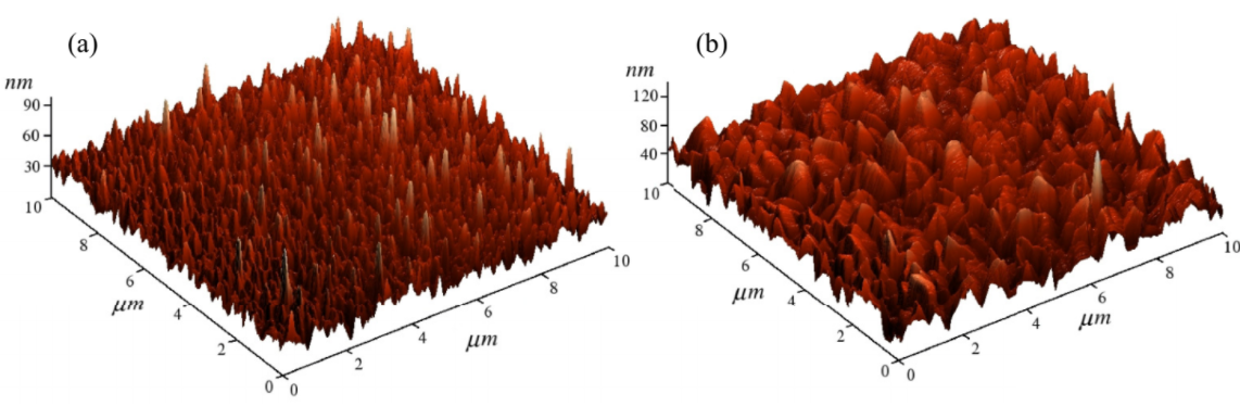
Figure 8: The surface morphology growth for polycrystalline CdTe/Si(100) films. AFM images for for a sample of size $10\mu m$ $\times$ $10\mu m$ $\times$, for deposition times $(a)$ $t$ $=60$ min; $(b)$ $t$ $=240$ min. From Almeida et al Almeida14 . With permission from PRB.

The experimental scenario to explore the mutation and propagation of bacteria is very rich with lot of possibilities. Thus is important to mention some quite interesting results Fusco16 in expanding populations revealed by spatial Luria–Delbrück. There the roughness front were measured and they reported that for flat front they have $z=2$, for both $1+1$ and $2+1$ dimensions, i.e. Edwards-Wilkinson universality class. For rough front $z=3/2$ for $1+1$ and $z=1.61$ for $2+1$ dimensions, i.e. the KPZ universality class, in agreement with GomesFilho21b .

II.4 Discrete growth model

To get a solution for the KPZ equation for $d+1$ dimensions is a big task for either analytical or numerical methods. Indeed, it is difficult even for $d=1$. On the other hand, there are a certain number of discrete models which operates by simple rules that can be easily implemented in a computer code. Such models are sometimes denominated cellular automata models Barabasi95 ; Mello01 ; Odor10 ; Almeida17 ; Reis05 ; Almeida14 ; Rodrigues15 ; Alves16 ; Carrasco18 ; Mello15 . To match some models into KPZ universality class is part of the scenario $c$.

As stated above, simulations of a cellular automaton is more simple and precise than the numerical solution of the KPZ equation itself. In this way, we show here two kinds of cellular automaton models that belong to the KPZ universality class.

II.4.1 The single step (SS) model

The single step (SS) model has gotten lot of importance along the years Krug92 ; Krug97 ; Derrida98 ; Meakin86 ; Daryaei20 : first, because it was proved to be a KPZ model, scenario $c$. Second, due to its connection with other models, such as the asymmetric simple exclusion process Derrida98 , the six-vertex model Meakin86 ; Gwa92 ; Vega85 , and the kinetic Ising model Meakin86 ; Plischke87 , it is a good example of the scenario $d$.

The SS model is defined in such way that the height difference between to neighbors heights $\eta=h_{i}-h_{j}$ is just $\eta=\pm 1$. Consequently, it is easily associated to the Ising model. For example for $1+1$ dimensions the initial conditions for the height of the site $i$ is of the form $h_{i}(0)=(1+(-1)^{i})/2$. Now, let us consider a hypercube of side $L$ and volume $V=L^{d}$. We select a site $i$, we compare its height with that of its neighbors and we apply the rules:

1. At time $t$ randomly choose a site $i\in{V}$;

2. If $h_{i}(t)$ is a minimum do $h_{i}(t+\Delta t)=h_{i}(t)+2$, with probability $p$

3. If $h_{i}(t)$ is a maximum do $h_{i}(t+\Delta t)=h_{i}(t)-2$, with probability $q$.

With the above rules we can generate the dynamics of the SS model for $d+1$ dimensions. For $1+1$ dimensions its properties have been well studied Krug92 ; Krug97 ; Derrida98 and we can obtain exact analytical results such as

$$\lambda=p-q.$$ (61)

Note that for $p=q$ it becomes the EW model. Changing the probabilities we can obtain quite a lot of relevant information Daryaei20 .

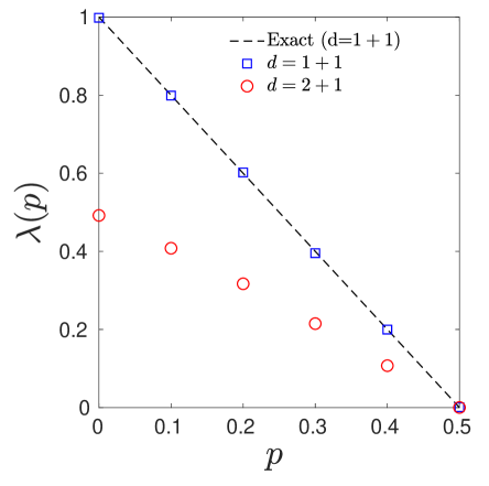
Figure 9: The parameter $\lambda$ as a function of the probability $p$, for the SS model. For $1+1$ dimensions we have the exact result $\lambda=p-q$; For $2+1$ dimensions $\lambda\propto(p-q)^{\delta}$, with $\delta=0.87(4)$. For $p=q$ we have the Edwards Wilkinson’s model. From Daryaei Daryaei20 , with permission of PRE.

In Figure (9) we show $\lambda$ as a function of the probability $p$. We exhibit the exact result for $1+1$ dimensions and the simulations for $2+1$ dimensions, here $p+q=1$. From Daryaei20 . Already in Figure (10), we show the snapshots of a typical surface morphology grown by SS for $2+1$ dimension, at the steady-state regimes, being $L=1024$ and $p$ ranges from $p=0$ the “best” KPZ regime to $p=0.5$, i.e. $\lambda=0$, which characterizes the EW regime.

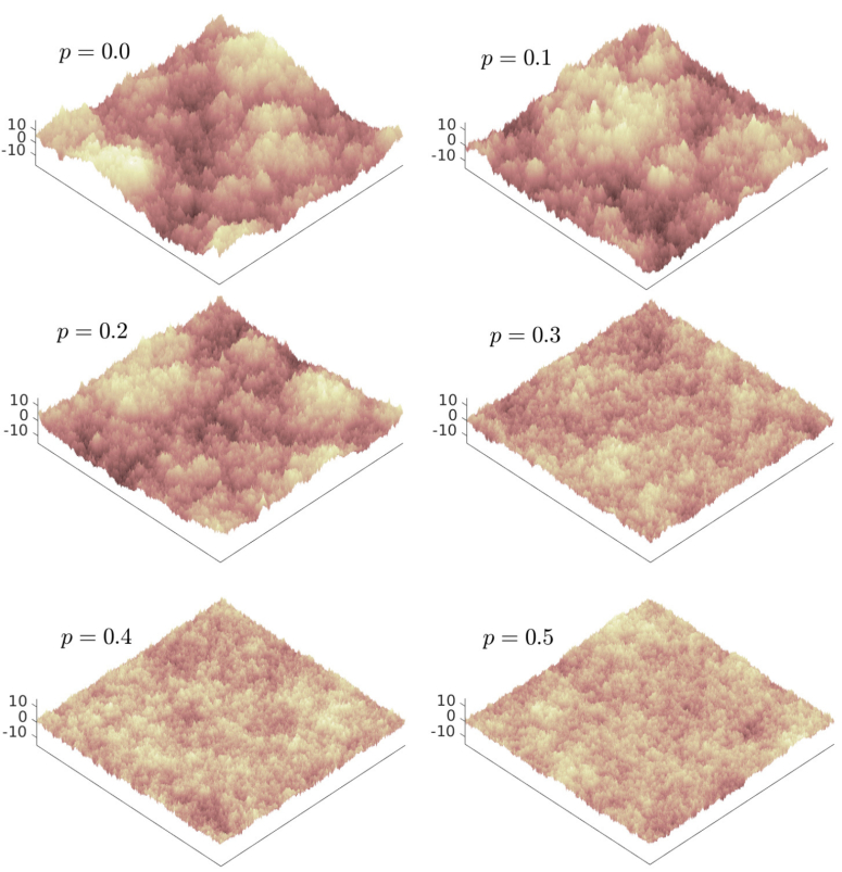
Figure 10: The surface morphology growth for the SS model for some values of $p$. We show here a lattice of size $1024$ $\times$ $1024$. From Daryaei  Daryaei20 . With permission from PRE.

II.4.2 The etching model

The etching model Mello01 ; Gomes19 ; Rodrigues15 ; Alves16 is a stochastic cellular automaton that simulates the surface erosion due to action of an acid. This model is proposed as simple as possible in order to capture the essential physics, which considers that the probability of removing a cell is proportional to the number of the exposed faces of the cell (an approximation of the etching process). First, we randomly select a site $i$ with a certain height, $h_{i}$ and then we compare it with one of its nearest neighbor $j$. This is similar to the SS model. Now the rules change If $h_{j}>h_{i}$, it is reduced to the same height as $h_{i}$, which means that the height of the surface decreases at each step. The main algorithm steps are summarized as follows:

1. At time $t$ randomly choose a site $i\in{V}$;

2. If $h_{j}(t)>h_{i}(t)$ do $h_{j}(t+\Delta t)=h_{i}(t)$;

3. Do $h_{i}(t+\Delta t)=h_{i}(t)-1.$

This stochastic cellular automaton has the advantage of allowing us to understanding a corrosion process, and at same time to study the KPZ growth process. Note that the rule $1$ is common to all these models, it is equivalent to the random term $\xi(\vec{x},t)$ in the KPZ equation (58). The interaction between the neighbors are equivalent to diffusive, and the nonlinear term, lateral growth. However, both $\nu$ and $\lambda$ change the intensity for each model.

Now we apply the above rules to study the etching mechanics in a system in $1+1$ dimensions with size $L=200$. In order to illustrate the major characteristic of a standard evolution of the surface width, we present a typical curve of the roughness $w(t)$ as a function of time $t$ in Figure 7, from the reference Gomes19 . The results were averaged over the sites and over $1\times 10^{7}$ different simulations. They also considered systems with periodic boundary conditions. The time evolution of the roughness dynamics, $w(t)$, presents four different regimes: $(a)$ at the beginning of the process (without correlations), $t<t_{0}\approx 5$, the mechanism is classified as random deposition, $w(t)\approx t^{1/2}$, that is, basically normal diffusion; $(b)$ the second region, $5<t<70$, the system had enough time for the correlation to reach distant points of the lattice, and the roughness is described by a power law dependence, $w(t)\approx t^{\beta}$; for $t$ between $70$ and $400$ the system passes through an intermediate region $(c)$; and last region $(d)$, for times higher than $400$, when the system reaches the saturation region $w(t)\approx w_{s}$. They obtained three major results from the figure: the characteristic time $t_{\times}=167.0(2)$; the saturation roughness $w_{s}=7.5228(6)$ for $t>>t_{\times}$; and the exponent $\beta$ was found equal to $0.334(3)$, which is much close to the Kardar-Parisi-Zhang (KPZ) exact value ($1/3$).

As an example of obtained the KPZ equation from a discrete model, Gomes et al. Gomes19 have recently developed a procedure which was successfully applied to the etching model above.

To obtain the KPZ equation from the etching model, we follow the procedure: First, we define $P(\eta,t)$ as the probability distribution that if at time $t$ a given site $i$ has height $h_{i}$ its neighbor must have height $h_{i}+\eta$, i.e., $\eta=h_{i}-h_{j}$ is the height difference between two neighbors sites.

Finally, we apply the rules of the etching model to obtain the KPZ equation with the coefficients as in Gomes19 :

$$D=\omega_{0}d,$$ (62)

where $\omega_{0}=1/\Delta t$ is the frequency of the noise, which is the frequency that drives all processes and appears in all coefficients. The linear dependence in $d$ is like in the diffusion models Oliveira19 ; Santos19 . Note that for the KPZ type of model $P(\eta,t)$ stabilizes very fast and, thus, it can be considered time independent for all regions of interest Gomes19 , consequently $P(\eta,t)=P(\eta)$. Then, we have as well that:

$$\nu=\frac{\omega_{0}d}{2}P(0)=\frac{P(0)}{2}D,$$ (63)

and

$$\lambda=2\omega_{0}d\frac{dP(\eta=0^{+})}{d\eta}=2D\left(\frac{dP(\eta)}{d\eta}\right)_{\eta=0^{+}}.$$ (64)

Thus, the equations (62) to (64) establish a very important relation between the KPZ parameters $\lambda$ and $\nu$ and $P(\eta)$, which shows that both KPZ parameters depend on the lateral growth and they are more than phenomenological parameters Gomes19 .

It should be noted that the increase of $\lambda$ with the dimension is a strong argument supporting Eq. (59), since this shows that $\lambda$ drives the other parameters. This method can be useful for other models of cellular automata.

Therefore, this was an example of a cellular automaton model for growth and of the recent method used to obtain the KPZ equation from it. Moreover, it obtains the coefficients $\nu$, $D$ and $\lambda$. The values of coefficients changes with the model and dimensions while the exponents $\alpha$, $\beta$ and $z$ are universal and depend only of the dimensions $d$. For the etching cellular automaton the coupling constant $g$ becomes

$$g=\frac{D\lambda^{2}}{\nu^{3}}=\frac{32}{P(0)^{3}}\left(\frac{dP(\eta)}{d\eta}\right)^{2}_{\eta=0}=\frac{32}{P(0)}\left(\frac{d\ln(P(\eta))}{d\eta}\right)^{2}_{\eta=0}.$$ (65)

This is the ultimate goal of statistical physics be able to express a given quantity in terms of probabilities Gomes19 . Unfortunately, such method is only for the etching model it would be very interesting if similar proposal could be done for other models.

Different methods and different models may show us some new features, the deep and the beauty of the KPZ dynamics. However, the major limitation of the method is that we do not have an analytical expression for $P(\eta)$. The search for it would bring a considerable evolution to the field.

II.4.3 Universal properties of the growth models

The universality goes beyond the set of critical exponents, reaching the height distributions, spatial and temporal correlations. In the last years, it was shown that these other universal quantities have a dependency with the interface geometry (see Kriecherbauer10 ; Halpin-Healy15 for recent reviews), where circular and linear interfaces displayed different statistics. Latter, simulations of flat surfaces that enlarged in time pointed out that the dynamic of the system size was the real responsible for the subdivision. Note that while a linear interface has a fixed lateral size, the perimeter of a circular one grows with its radius.

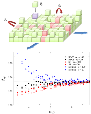
Figure 11: (Up) Illustration of the substrate enlargement and deposition for $2+1$ dimensions. (Down) The evolution of the exponent $\beta$ as function of $t$ for $1+1$ dimensions. From Carrasco et. al  Carrasco14 . With permission from NJP.

For instance, Figure (11) illustrates the lateral enlargement for simulations in $2+1$ dimensions. At each time step, there is a chance of particle deposition with probability $P_{d}=\frac{N}{N+\omega d_{s}}$, and a probability $P_{a}=\frac{\omega d_{s}}{N+\omega d_{s}}$ for the system to enlarge through the duplication of a row or a column, see Carrasco14 for more details. Here $N$ is the total number of sites $d_{s}=d+1$, i.e. the “full” volume, and $\omega$ the enlargement rate, i.e. the size evolves as $<L(t)>=L_{0}+\omega t$. Even without any curvature, only the addition of these lateral duplications was enough for the system to show the statistics of the curved KPZ subclass. The irrelevance of the geometry in the subdivision was confirmed when experiments of curved interfaces that shrink in time showed the statistics of the flat KPZ subclass (Fukai17 and further discussed in Carrasco18 ; Carrasco19 ). Already in Figure (11) down, we showed the values of $\beta$ as function of $t$ for some models in $1+1$ dimensions. Here $\beta(t)=\frac{d\ln{[W(t)]}}{dt}$. We see the convergence for $\beta=1/3$, as it should be for the KPZ universality class in 1+1 dimension.

II.5 One FDT for KPZ

A second look at Eqs. (63) and (64) exhibit not only the dependence on $P(\eta)$, but it also shows in a very direct way that the parameters $\lambda$ and $\nu$ are driven by the noise $D$. This shows that fields in the right hand of Eq. (58) are from the same source. Moreover, it is a form of Fluctuation-dissipation theorem associated Gomes19 with the parameters of a solid on solid model. This was a first step towards the understanding of the rule of the fluctuation-dissipation theorem in growth.

For the KPZ equation the FDT works only in $1+1$ dimensions Kardar86 ; Rodriguez19 . The major question is that in the Langevin’s equation both the fluctuation and the dissipation are part of the same force due to the thermal bath. This is not clear for the growth phenomenon. In a recent article GomesFilho21 the saturation mechanism, i.e. $w(t\rightarrow\infty)=w_{s}$ was demonstrated to be similar to the thermalization mechanism in the Langevin’s equation.

For the EW and KPZ equation we have as well that the noise increases $h$ and $w(t)$ linearly with time, while the term $\nu\nabla^{2}h(\vec{x},t)$, which is always opposite to roughness, decreases it. The roughness increases with time until it reaches saturation, which, for $1+1$-dimensional systems, is given by the exact results:

$$w_{s}=\sqrt{\frac{cD}{\nu}L},$$ (66)

where $c=1/(4\pi^{2})$ for Edwards-Wilkinson Edwards82 and $c=1/24$ for the single step (SS) model Krug92 ; Krug97 . For growth, we do not have an equipartition theorem, but we have $w^{2}(t\rightarrow\infty)=w_{s}^{2}$, which is equivalent to $\left\langle v^{2}(t\rightarrow\infty)\right\rangle=k_{B}T/m$. Thus, by replacing $D$ by the above value, Eq. (56) becomes:

$$\left\langle\xi({x},t)\xi({x^{\prime}},t^{\prime})\right\rangle=2b\nu w_{s}^{2}\delta({x}-{x^{\prime}})\delta(t-t^{\prime}),$$ (67)

with $b=1/(cL)$. Therefore, the parameter $D$ in Eq. (56) is not only the noise intensity, but it is also related to $\nu$, in the above equation, which leads to a fluctuation-dissipation theorem. Note the similarity between Eq. (67) and Eq. (19). Also, since the noise and the surface tension in the Edwards-Wilkinson equation have their origin in the flux, the separation between them is artificial, consequently, the above discussion restore the lost link GomesFilho21 ; Anjos21 .

II.6 The quest for the KPZ exponents

The search for the KPZ exponents has been one for more than three decades. For $1+1$ dimensions the Group Renormalization (RG) method Kardar86 yield the $\alpha=1/2$, $\beta=1/3$ and $z=3/2$. However, the RG method does not give correct results for $d\geq 2$. Since Eq. (54) and Eq. (59) relate the three exponents, we only need to determine one of them to obtain information about all of them. Therefore, in the next subsections, we will focus on determining the value of $\alpha$.

Based on empirical data Wolf and Keztesz Wolf87 proposed

$$\alpha(d)=\frac{1}{d+1},$$ (68)

while Kim and Kosterlitz Kim89 have proposed

$$\alpha(d)=\frac{2}{d+3}.$$ (69)

With the development of better computational tools and machines, simulations have shown values that diverge from both proposals. Lassig Lassig98 have proposed a field theoretical method which yielded $\alpha(2)=2/5$, and $\alpha(3)=2/7$, again they are far from the simulations results. Up to now we can resume theoreticals attempts as:

1. Scaling fails for all dimensions.

2. RG gives exact results only for $1+1$ dimensions Kardar86 .

3. Field theoretical methods yield exponents that are not precise Lassig98 ; Sun94 .

The RG approaches does not give precise exponents for $d+1$ dimensions for $d\geq 2$. However, some calculations using RG produces very useful results. For example, Canet et al Canet10 ; Canet11 used nonperturbative RG and obtained the only complete analytical approach yielding a qualitatively correct phase/flow diagram to date.

In the next subsection we shall consider what is particularly valid in these approaches and we shall add three important ingredients: First, we use dimensional analysis which is always a strong tool; Second, the fractal dimension of the interface replacing the Euclidean integer dimension; Finally, a proper correction of the fluctuation dissipation theorem for higher dimensions.

II.7 The KPZ exponents in $2+1$ dimensions

The attempt to obtain the exact exponents for the KPZ equation, as exposed above is one of the major objective in the area. However, so far it has not been achieved. Since $2+1$ dimensions corresponds to our three dimensional space this is physically the most important dimension. Thus we call attention to some recent proposals for the KPZ exponents GomesFilho21b ; Oliveira22 . The major idea is that while the space dimension is $\tilde{D}=d+1$, the interface dimension $D_{i}$ where the growth occurs is fractal Anjos21 given by $D_{i}=d_{f}+1$. The fractal nature of the interface is evident in Figure (10) and the experimental results in Figure (8), as previously reported in the literature, it is connected with the roughness exponent $\alpha$ by Barabasi95 :

$$\alpha=2-d_{f},$$ (70)

for $d=1,2$. Note that we need a second relation connecting $\alpha$ and $d_{f}$ to obtain ($d_{f},\alpha,\beta,z)$. This relation was provided by Gomes-Filho et al as  GomesFilho21b

$$\alpha=\frac{1}{\tilde{d}_{f}+1},$$ (71)

where $\tilde{d}_{f}$ is the fractal dimension seen by the effective fluctuation after selecting the fractal surface Anjos21 , where $d-1\leq\tilde{d}_{f}\leq d$. In other words, the available fractal dimension for the noise is smaller than the space dimension. In the case of $d=1$, the only possibility is $\tilde{d}_{f}=1$, resulting in $\alpha=1/2$. For $d=2$, a good approximation is $\tilde{d}_{f}=d_{f}$, which allows one to obtain the KPZ exponents in 2+1 dimensions  GomesFilho21b :

$$z=d_{f}=\frac{1+\sqrt{5}}{2},\hskip 19.91684pt\alpha=\frac{3-\sqrt{5}}{2},\hskip 19.91684pt\beta=\sqrt{5}-2.$$ (72)

It is interesting to mention that these exponents are consistent with different experimental results. A better agreement was achieved with experiments that measure the exponent $z$. For instance, accurate experiments have reported values of $z$ as $1.6(2)$ Orrillo17 , $1.6(1)$ Ojeda00 , $1.61(5)$ Almeida14 , and $1.61(2)$ Fusco16 , which are in agreement with the value of $z=d_{f}=\frac{1+\sqrt{5}}{2}=1.61803...$ Recent simulation results Luis22 ; Luis23 further support these findings, as they have obtained similar values of $d_{f}$ by the use of different methods.

Moreover, the exponents are as well in a good agreement with simulations. For instance, the average over $20$ different methods and models GomesFilho21b gives $\overline{\alpha}=0.3828\pm 0.0037$, which agrees well with $\alpha=\frac{3-\sqrt{5}}{2}=0.381966011$. It is worth mentioning that T. Oliveira Oliveira22 recently reported precise values of $\alpha=7/18$ and $\beta=7/29$ for $2+1$ dimensions, which yield a calculated value of $d_{f}=1.611...$, very close to the previously mentioned one. It should be noted however that the approach presented in Oliveira22 relies on the Ansatz (Eq. (8) in Ref.Oliveira22 ) which is an unproven relationship. Therefore the search for the exact KPZ exponents has not been finished yet.

II.8 There is no Upper Critical Dimension for KPZ

The study of a model in dimensions higher than $2+1$ has some theoretical importance, including the investigation of the existence of an upper critical dimension (UCD) where the exponents do not change anymore. This concept is well-known in the case of the Ising model, which has a UCD of 4. Simulations Alves14 ; Rodrigues15 ; Odor10 suggest that if a UCD exists for the KPZ universality class, it must be for $d>6$. However, we can prove the non-existence of a UCD. Consider $d>2$, Eq. (71) with $d-1\leq\tilde{d}_{f}\leq d$ imposes the limit

$$\frac{1}{d+1}\leq\alpha=\frac{1}{d_{f}+1}\leq\frac{1}{d},$$ (73)

which means that as $d$ changes, the allowed values for the exponents also change. Consequently, there is no UCD for KPZ.

As mentioned above, the wide application of the methods developed for KPZ dynamics and the large number of models associated with it, as well as the new wave of quantum phenomena recently mapped Corwin18 ; Nahum17 ; Ljubotina19 ; DeNardis19 into KPZ, makes it one of the biggest problems in statistical physics. This shows how central this question is, and how far we are from exhausting the topic.

III The Quantum Fluctuations Theorems

The convenient Langevin framework can be rephrased in quantum-mechanical theory exploring the concept of the environment (the heat bath) modeled in terms of free harmonic oscillators Ford ; Ford1 ; Caldeira83 . By using general physical principles, as causality and uniqueness of the equilibrium state, the macroscopic Langevin-like equation corresponding to a reduced description of the system can be derived. It should be stressed, however, that this approach (called “phenomenological” by Van Kampen vanKampen92 ; vanKampen97 ) is neither unique nor straightforward, as “in quantum mechanics one needs to take into account the physical origin not only of the fluctuations but also of the damping” vanKampen97 .

Over the past century, the linear response theory of quantum systems to applied external perturbations have been advanced inspired by the works of Nyquist, Johnson, Kubo and Callen Nyquist28 ; Johnson28 ; Takahashi52 ; Kubo57 ; Kubo57a ; Callen51 ; Callen52 . In particular, it has been established that the linear response coefficients in Hamiltonian systems are proportional to two-point correlation functions Kubo57 ; Kubo57a , similarly to situations arising in stochastic systems, as described in Subsection 1.3.

Further extensions and relation to thermodynamics have been developed by Onsager Onsager31 who studied relaxation dynamics of the macroscopic system observable in terms of the first (time) derivative of entropy, which is nonzero away from equilibrium. According to Onsager’s definition, the derivative of entropy with respect to a macroscopic variable is termed the thermodynamic force which in this scenario is coupled linearly to a thermodynamic flux by a kinetic coefficient. In his seminal work Onsager presented also a proof of the symmetry relations in the kinetic coefficients and established a link between dispersion of fluctuations and relaxation rates. It took several decades for a new series of developments, reflecting, among others, context of stochastic thermodynamics of mesoscopic systems, linear response of non-Markov processes and response of stochastic processes driven by non-Gaussian fluctuations  Costa03 ; Hanggi90 ; Deker75 ; Kubo74 ; Kubo91 ; Ruelle98 ; Zwanzig01 ; Seifert12 ; Dybiec12 ; Dybiec17 ; Nowak14 ; Marconi08 ; Sarracino19 ; Winkler20 . Another generalization of the fluctuation-dissipation relations stems from the pioneering work of Bochkov and Kuzovlev Bochkov77 ; Bochkov81 who obtained rigorous equalities for fluctuations (fluctuation theorems) in an arbitrary system brought up to a strongly nonequilibrium state. Their work has been further followed by Jarzynski Jarzynski97 ; Jarzynski00 and Crooks Crooks99 . Notably, in contrast to fluctuation-dissipation relation studied in linear regime, the fluctuation theorems provide information about the nonlinear response and have been tested experimentally Saira12 .

III.1 Mori’s equation and the Kubo’s fluctuation-dissipation theorem

For a system described by a quantum operator $A$, Mori Mori65 ; Mori65a ; Kubo74 ; Zwanzig01 developed a method which generalizes the Langevin’s equation to take the form

$$\frac{dA(t)}{dt}=-\int_{0}^{t}\Gamma(t-t^{\prime})A(t^{\prime})\,dt^{\prime}+F(t),$$ (74)

where $F(t)$ is a stochastic noise subject to the conditions:

$$\langle F(t)\rangle=0,$$ (75)

$$\langle F(t)A(0)\rangle=0$$ (76)

and

$$C_{F}(t-t^{\prime})=\langle F(t)F(t^{\prime})\rangle=\langle A^{2}\rangle_{eq}\Gamma(t-t^{\prime}).$$ (77)

The above equation (74) is called generalized Langevin equation or Mori’s equation. Note that both Eqs. (75) and (76) are similar to the Langevin equation (Eqs. (14) and (15)). However, the third condition, Eq. (77), exhibits a more general behavior. For example, consider now the particular case $A(t)=mv(t)$ and

$$\Gamma(t)=2\gamma\delta(t)$$ (78)

then the generalized Eq.(74) becomes the standard Langevin’s equation (11). The existence of the memory kernel, $\Gamma(t)$, indicates that each step depends on the previous ones. The noise is random, but with some inherent memory, which correlates events of a fluctuating force $F(t)$ executed on the system at hand. In such situations, we say that the process is non-Markovian and Eq. (77) is the Kubo FDT Kubo91 ; Kubo66 . The Mori formalism with the Kubo FDT yield the Generalized Langevin equation (GLE), Eq. (74). On the other hand, Lee Lee83 ; Lee82 ; Lee83a ; Lee84 derived a recurrence relation method, which is an alternative to the Mori’s method for projection operators. Derivation of correlations functions is nowadays an important part of research in the field Nowak22 ; Florencio20 ; Chen20 ; Feng20 ; Reggiani20 ; Maes20 ; Fotso20 ; Wu20 .

III.1.1 Response functions

As we have seen in the Langevin framework the correlation function, Eq. (22), is fundamental for the determination of the dynamics. For the Mori equation, the correlation function has been a subject of intense investigation Florencio85 ; Lee83 ; Lee82 ; Lee84 . Thus, let us define the response function:

$$R(t)=\frac{C_{A}(t)}{C_{A}(0)},$$ (79)

where,

$$C_{A}(t)=\left\langle A(t)A(0)\right\rangle.$$ (80)

We can study the diffusive properties of the operator $A(t)$ by defining

$$x(t)=\int_{0}^{t}A(s)ds,$$ (81)

thus we can define a diffusive behavior for $x(t)$ whatever that is. Now we consider Eq. (10), replacing $D$ by $D(t)$ with

$$D(t)=\int_{0}^{t}C_{A}(t^{\prime})dt^{\prime}.$$ (82)

Note that $D(t)$ may not converge to a constant as in the Langevin’s case. Taking the dispersion in the asymptotic regime, $t\to\infty$, as

$$\sigma_{x}^{2}=\left\langle(x-\left\langle x\right\rangle)^{2}\right\rangle\sim D(t)t\sim t^{\alpha},$$ (83)

where $\alpha$ defines the type of diffusion. For $\alpha=1$ we have the normal diffusion, which draws a line between the subdiffusion $0<\alpha<1$ and superdiffusion $\alpha>1$.

Now if we multiply the Eq. (74) by the set of $A(0)$ and take the ensemble average, we obtain a self-consistent equation for $R(t)$, namely

$$\frac{dR(t)}{dt}=-\int_{0}^{t}R(t-t^{\prime})\Gamma(t^{\prime})dt^{\prime}.$$ (84)

Once we determine $R(t)$, we are able to give a full description of all system. There is a great evolution going from (74) to (84). From (74) we have to simulate a large number of trajectories to get a reasonable result. On the other hand, from (84) we just have to solve an equation, which allows analytical solutions, as we shall see below.

First, let us consider the nature of the noise, which can be associated with a set of harmonic noise of the form Morgado02 ; Hanggi90

$$F(t)=\left(2\langle A^{2}\rangle_{eq}\right)^{1/2}\int_{0}^{\infty}\sqrt{\rho(\omega)}\cos[\omega t+\phi(\omega)]d\omega,$$ (85)

where the random phases, $0\leq\phi(\omega)\leq 2\pi$, provide the stochastic character. We now insert $F(t)$ into Eq. (77) to obtain:

$$\Gamma(t)=\int\rho(\omega)\cos(\omega t)d\omega,$$ (86)

being $\rho(\omega)$ the noise density of states. The memory is even for any noise distribution Vainstein05 . Note that for a classical system $\langle A^{2}\rangle_{eq}\propto T$ and the noise (85) is due to thermal fluctuations. Note as well that

$$\frac{dR(t)}{dt}\biggr{|}_{t=0}=0,$$ (87)

as it must be from Eq. (84). As an example of noise density, we propose:

$$\rho(\omega)=\begin{cases}\frac{2\gamma}{\pi}\left(\frac{\omega}{\omega_{1}}\right)^{\nu},&\text{ if }\omega<\omega_{1}\\ \frac{2\gamma}{\pi},&\text{ if }\omega_{1}<\omega<\omega_{2}\\ 0,&\text{ if }\omega>\omega_{2}.\end{cases}$$ (88)

The constant in the density is chosen in such way that for normal diffusion, $\widetilde{\Gamma}(z=0)=\gamma$, see below. This noise spectrum contains most of the noise discussed in the literature Costa03 ; Vainstein06a ; Morgado02 ; Vainstein05 ; Ferreira12 . Note that if $\omega_{1}=\omega_{2}$ it becomes a Debye cutoff frequency. We shall consider now three kinds of noise:

$(i)$ For $\nu=0$, we have Morgado02

$$\Gamma(t)=\frac{2\gamma\omega_{2}}{\pi}\left[\frac{\sin(\omega_{2}t)}{\omega_{2}t}\right],$$ (89)

which yields a normal diffusion Morgado02 . Note that if $\omega_{2}\rightarrow\infty$ we recover the white noise spectrum and $\Gamma(t)\rightarrow 2\gamma\delta(t)$. Laplace transforming Eq. (89) we get

$$\widetilde{\Gamma}(z)=(2\gamma/\pi)\arctan(\omega_{2}/z).$$ (90)

Now, a new time scale $t_{2}=\omega_{2}^{-1}$ arises naturally. For $t>>t_{2}$, which is equivalent to $\widetilde{\Gamma}(z\rightarrow 0^{\pm})=\pm\gamma$, $R(t)$ does not shows any deviation from $R(t)=\exp(-\gamma|t|)$, which means the memoryless Langevin equation. However, its short time behavior, $0<t<t_{2}$, is quite different.

$(ii)$ For $\nu=1$ and $\omega_{1}=\omega_{2}$, we get Ferreira12

$$\Gamma(t)=\left(\frac{2\gamma\omega_{1}}{\pi}\right)\left[\frac{\sin(\omega_{1}t)}{\omega_{1}t}+\frac{1-\cos(\omega_{1}t)}{(\omega_{1}t)^{2}}\right],$$ (91)

with Laplace transform equal to:

$$\widetilde{\Gamma}(z)=\left(\frac{\gamma z}{\pi\omega_{1}}\right)\ln\left[1+\left(\frac{\omega_{1}}{z}\right)^{2}\right],$$ (92)

For $\lim_{z\rightarrow 0}\widetilde{\Gamma}(z)\propto-z\ln{z}$, which yields a weak ballistic behavior Ferreira12 . For example, in Figure (12) we show the correlation function obtained from the above memory.

($iii)$ Finally, considering $\nu\rightarrow\infty$, we get

$$\Gamma(t)=\left(\frac{2\gamma}{\pi t}\right)\left[\sin(\omega_{2}t)-\sin(\omega_{1}t)\right],$$ (93)

which yields $\lim_{z\rightarrow 0}\widetilde{\Gamma}(z)\propto z$, i.e. ballistic diffusion Morgado02 ; Costa03 . The above memories are not an artificial construction. For example (93) was used successfully to describe the dynamics of spin wave diffusion in a random-exchange Heisenberg chain Vainstein05 ; Vainstein05a .

In this sense, the motivation for considering such cases will become clear below.

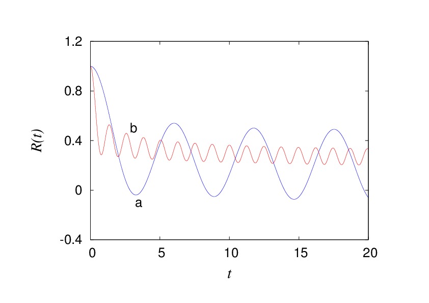
Figure 12: Correlation function $R(t)$ as function of $t$ in arbitrary units. We use the memory (93) and we integrate numerically Eq. (84): (a) $\gamma=\frac{\pi}{2}$ and $\omega_{1}=1$; (b) $\gamma=\frac{5\pi}{4}$ and $\omega_{1}=5$. From ref. Ferreira12 , with permission from PRE.

III.1.2 Exact solutions for anomalous diffusion

The major objective in any field of physics is to obtain exact results. Thus, in this section we determine the exact exponents for anomalous diffusion.

Then from Eq. (82) we have

$$\lim_{t\rightarrow\infty}D(t)=\lim_{z\rightarrow 0}\int_{0}^{t}C_{A}(t^{\prime})\exp(-zt^{\prime})dt^{\prime}=C_{A}(0)\lim_{z\rightarrow 0}\tilde{R}(z).$$ (94)

The tilde denotes the Laplace transform, in the last part we use the final-value theorem Morgado02 . Considering that $z\propto 1/t$, we find the asymptotic behavior of $D(t)$.

Furthermore, by applying the Laplace transform to equation (84), we obtain

$$\widetilde{R}(z)=\frac{1}{z+\widetilde{\Gamma}(z)}.$$ (95)

Further analysis of the above equation allows one to obtain information about the asymptotic behavior of the system. Since we know $\widetilde{\Gamma}(z)$, we can get the resulting dynamics. For instance, considering that $\lim_{z\rightarrow 0}\widetilde{\Gamma}(z)\propto z^{\mu}$, then the anomalous diffusion, $D(t)$, Eq. (94) becomes

$$\lim_{t\rightarrow\infty}D(t)\propto t^{\beta}$$ (96)

and therefore the diffusion exponent $\alpha$ is given by Morgado02 :

$$\alpha=\beta+1,$$ (97)

being

$$\beta=\begin{cases}\mu,&\text{ if~{}~{} }-1<\mu<1\\ 1,&\text{ if~{}~{} }\mu\geq 1,\\ \end{cases}$$ (98)

so the exponent $\beta$ is limited in a specific range implying that the diffusion exponent $\alpha$ is limited as well.

Most works Metzler00 ; Metzler04 ; Morgado02 ; Morgado04 have analyzed only the asymptotic behavior of the diffusion as the power law described by Eq. (83). Ferreira et al. Ferreira12 ; Ferreira22 prove that $z\propto 1/t$ as $t\rightarrow\infty$ is exact. More precisely, they define the scaling

$$z=\frac{\lambda(t)}{t},$$ (99)

and proved that

$$\lambda(t)=1-\lim_{t\rightarrow\infty}t\frac{d}{dt}\ln{[f(t)]},$$ (100)

with

$$f(t)=1-t\tilde{\Gamma}\left(\frac{\lambda(t)}{t}\right).$$ (101)

These relations works not only for large values of $t$, but as well for intermediate values Ferreira22 .

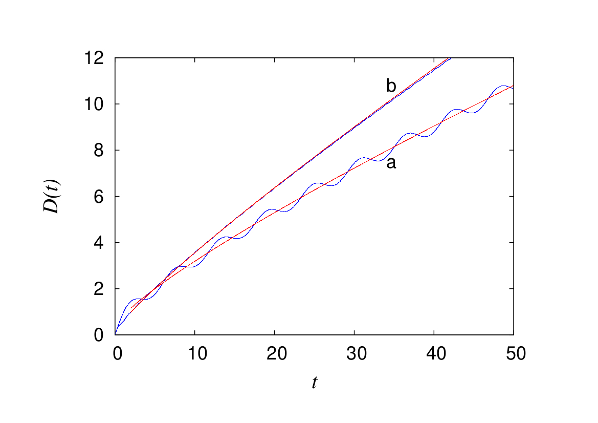
Figure 13: Evolution of $D(t)$ as function of $t$ We use the memory (93). we integrate numerically Eq. (84), and then Eq. (82) with $\gamma=\frac{\pi}{2}$. (a) $\omega_{1}=1$ and $\omega_{2}=2$; (b) $\omega_{1}=3$ and $\omega_{2}=4$. The curves with oscillations are obtained by numerical integration of Eq. (84), and then Eq. (82). The curves without oscillations are these obtained by using (100). For small oscillations (b) the curves superimpose. From ref. Ferreira12 , with permission from PRE.

In Figure (13) we exhibit the evolution of $D(t)$ using the correlation function obtained from Figure (12). It is clear that $D(t)$ grows up with time without convergence to a fixed limit. This is a supper diffusive behavior.

They consider as well a generalization of Eq. (83) as

$$\lim_{t\rightarrow\infty}\left\langle r^{2}(t)\right\rangle\sim t^{\alpha}\left[\ln(t)\right]^{\pm n}\sim t^{\alpha^{\pm}}.$$ (102)

Thus, we have $\alpha^{\pm}$ diffusive behaviors. This definition for $\alpha^{\pm}$ exponents was inspired in the critical exponents of a phase transition. For instance, in magnetic systems with null external field, $H=0$, for temperatures $T\approx T_{c}$, the specific heat behaves as $C_{H=0}\propto|T-T_{c}|^{-\alpha}$, being $\alpha$ the critical exponent. As it is well known for the Ising model, in two dimensions $C_{H=0}\propto\ln{|T-T_{c}|}$ thus we say that $\alpha=0^{+}$. This generalization exhibits the wideness of the diffusive behavior. As an example for $t\rightarrow\infty$, an anomalous behavior of the form $\langle x^{2}(t)\rangle\propto\frac{t}{\ln(t)}$ was proposed by Srokowski Srokowski00 ; Srokowski13 . Thus, in our notation has $\alpha=1^{-}$, and it is a weak form of subdiffusion. In this way the diffusive exponents can be cast in the form:

$$\alpha=\begin{cases}2,&\text{ if~{}~{} }\nu>1\\ 2^{-},&\text{ if~{}~{} }\nu=1\\ 1+\nu,&\text{ if~{}~{} }-1<\nu<1.\end{cases}$$ (103)

Now we see two different kinds of ballistic motion, with the diffusion exponent $\alpha=2^{-}$ and $\alpha=2$. The weak ballistic motion $\alpha=2^{-}$ is ergodic while the ballistic case $\alpha=2$ is not Lapas08 . Obviously, this difference does not appears easily in numerical simulations, however a proper analytical analysis shows it systematically Lapas08 ; Lapas07 ; Ferreira12 . Note that all diffusion discussed here are in the absence of an external fields, which would alter the results.

This formalism can also help us study the heat transfer between nanoparticles separated by a distance of the order of a few nanometers. Thermal fluctuations can excite the surface waves (electromagnetic eigenmodes of the surface) inside a body. The intensity of surface waves is many orders of magnitude larger in the near-field than in the far-field, being quasi-monochromatic in the vicinity of the surface Joulain05 . For near-field interactions, one can calculate the thermal conductance under the assumption that both NPs behave as effective dipoles at different temperatures Domingues05 . Since these dipoles undergo thermal fluctuations, the FDT can provide the energy, which dissipates into heat in each NP. In a more general framework Perez-Madrid08 , the thermal conductance can be computed by assuming that the particles have charge distributions characterized by fluctuating multipole moments in equilibrium with heat baths at different temperatures. This quantity follows from the FDT for the fluctuations of the multipolar moments.

IV limits of the Kubo formalism

The Kubo formalism is a strong, exact method to determine various material properties and transport coefficients, like e.g. conductivity, from a properly chosen autocorrelation functions and has been used in a large number of applications. Now we shall ask a few general question considering limitations of this framework.

IV.1 Entropy and the second law of thermodynamics

The first question is about the second law of thermodynamics for stochastic process. We do expect that the second law to be always valid. But, can we prove it for the stochastic formalism presented here?

This question was brought up and discussed by several authors, see e.g. Seifert12 ; Dybiec17 ; Lapas07 . In Ref. Lapas07 the total variation of entropy $\Delta S$ was computed in the diffusion process and associated with the behavior of the memory kernel $\Gamma(t)$: Consider that

$$\tilde{\Gamma}(z\rightarrow 0)\rightarrow bz^{\nu},$$ (104)

where the effective values of $\nu$ are in the range $-1\leq\nu\leq 1$. For $-1\leq\nu<1$ the variation of entropy $\Delta S$ during the process is automatically positive. For $\nu=1$ the condition was that

$$b=\int_{0}^{\infty}\frac{\rho(\omega)}{\omega^{2}}d\omega>0,$$ (105)

where $\rho(\omega)$ is the spectral density in Eq. (86). Since $\rho(\omega)>0$, the two equations above clearly indicate that the positivity of $\Delta S$ for long times is secured and the second law of thermodynamics is fulfilled, as expected. It is quite interesting to notice that a canonical form of the heat reservoir (a system of linearly coupled oscillators) responsible for the expression Eq.(84) is sufficient to guarantee the requirement of the second law.

IV.2 Khinchin theorem, ergodicity and violation of the FDT

The ergodicity concept, which has a wide impact in statistical physics, has been first introduced in the form of hypothesis by Boltzmann Boltzmann74 . The ergodic condition, Eq. (13), rephrased by Birkhoff and von Neumann for dynamic systems generating a flow in the phase space, asserted that the time average and the ensemble average taken over all possible states with the same energy are equal for all but negligible set of the states. A very important theorem related to the ergodic hypothesis is due to Khinchin Khinchin49 ; Lee07a . The Khinchin theorem states that, for a classical system, the ergodicity of a dynamic variable $A(t)$ in thermal equilibrium must hold if the autocorrelation function Eq.(80) satisfies

$$\lim_{t\rightarrow\infty}\left\langle A(t)A(0)\right\rangle=\left\langle A\right\rangle\left\langle A\right\rangle$$ (106)

It is noteworthy to mention that the theorem establishes also a relationship between the ergodicity and mixing condition. The mixing condition can be written as:

$$\lim_{t\rightarrow\infty}R(t)=0,$$ (107)

which means that, after a long time, the system forgets the initial conditions. Then, the Khinchin theorem states that if the mixing condition holds the Boltzmann ergodic hypothesis (BEH) holds as well. In the last decades, it has been addressed by some researches for systems described by the Mori formalism Costa03 ; Lapas07 ; Lapas08 ; Lee01 ; Lee07a . For example, consider the limit:

$$\lim_{t\rightarrow\infty}R(t)=\lim_{z\rightarrow 0}z\tilde{R}(z).$$ (108)

For systems described by the generalized Langevin’s equation, $\tilde{R}(z)$ is given by Eq. (95), and if we consider that as $z\rightarrow 0$ the leading term in $\tilde{\Gamma}(z)$ behaves as $\tilde{\Gamma}(z)\rightarrow bz^{\alpha-1}$, then we can write:

$$\Lambda=\lim_{t\rightarrow\infty}R(t)=\lim_{z\rightarrow 0}\frac{1}{1+bz^{\alpha-2}}.$$ (109)

Now, it is easy to see that, for $\alpha<2$, the mixing condition holds and the BEH holds, according to the Khinchin theorem. For the ballistic motion $\alpha=2$, $\Lambda=(1+b)^{-1}\neq 0$, and the mixing condition does not hold. Consequently, the BEH does not work. Thus, the factor $\Lambda$ is called the nonergodic factor Costa03 .

In this way, we can write a solution of Eq. (74), similar to the one written for the Langevin equation, Eq. (11), as

$$A(t)=A(0)+\int_{0}^{t}F(s)R(s)ds,$$ (110)

now we square and take a time average to reach

$$\overline{A^{2}(t)}=\langle A^{2}\rangle_{eq}+R(t)^{2}\left[\langle A^{2}(0)\rangle-\langle A^{2}\rangle_{eq}\right].$$ (111)

Note that if the system is initially at equilibrium $\langle A^{2}(0)\rangle=\langle A^{2}\rangle_{eq}$, it will remain in equilibrium forever, i.e., no fluctuation will drive it far from equilibrium. However, if the system is initially out equilibrium $\langle A^{2}(0)\rangle\neq\langle A^{2}\rangle_{eq}$, it will approach the equilibrium as $R(t\rightarrow\infty)=0$, which means, when the mixing condition Eq. (107) is obeyed. Otherwise, if the time average will be not equal to the ensemble average, the BEG does not work Costa03 . Thus, we arrived in a very important result:

• If $\Lambda=0$, the mixing condition holds and the BEH holds as well.

• If $\Lambda\neq 0$, the mixing condition does not holds and the BEH also fails.

In any of the above situations the Khinchin theorem works.

Using equations similar to Eqs. (110) and (111), we can also derive the moments of higher orders and define the non-Gaussian factor:

$$\eta(t)=\left[\frac{\langle A^{2}(0)\rangle}{\langle A^{2}(t)\rangle}\right]^{2}\eta(0)R^{4}(t),$$ (112)

and the skewness parameter Lapas07 ; Lapas08

$$\phi(t)=\left[\frac{\sigma_{A}(0)}{\sigma_{A}(t)}\right]^{3}\phi(0)R^{3}(t).$$ (113)

The non-Gaussian factor serves as a measure of deviation of the distribution of a stochastic variable $A(t)$ from a Gaussian statistics. Note that if $\eta(0)=0$, the distribution always will be a Gaussian. The asymmetry of the distribution given by $\phi(t)$ has a similar property. For example, if the initial $\phi(0)$ is null at the beginning, dynamics of the system will preserve symmetry of the distribution. If the initial distribution is non-Gaussian ($\eta(0)\neq 0$, $\phi(0)\neq 0$), both indicators evolve towards a more symmetrical final distribution for $t\rightarrow\infty$ (this is demonstrated by the ratio $\eta(t)/\eta(0)$ which is less than 1, as long as $R^{2}(t)<1$). Moreover, since $\lvert R(t)\rvert<1$, the process of ”Gaussianization” will occur much faster than decay of $R(t)$, for example if $R(t)/R(0)\approx 10^{-1}$, $\eta(t)/\eta(0)\approx 10^{-4}$. Moreover, if the mixing condition is fulfilled, the long-time distribution attains a Gaussians one.

As exposed above, the relation between fluctuations and dissipation plays a crucial role in the response theory grounded in statistical mechanics. The FDT formalism derived for close-to-equilibrium systems, where detailed balance holds, allows us to obtain important measured quantities such as susceptibility, the light scattering cross section, the neutron scattering intensity, diffusion, surface roughness in growth, etc. by studying spontaneous correlations of fluctuating dynamic variables. On the other hand breakdown of the equilibrium FDT is a very common fact, and it is well documented in the literature. For example, in the KPZ dynamics, the FDT works for $1+1$ dimensions, however, it fails for $d+1$ dimensions when $d>1$  Kardar86 ; Rodriguez19 . The violation of the FDT has been also observed in structural glass experiments, through extensive computer simulations Barrat98 ; Bellon05 ; Bellon02 ; Crisanti03 ; Grigera99 ; Ricci-Tersenghi00 , in proteins Hayashi07 , in mesoscopic radiative heat transfer Perez-Madrid09 ; Averin10 , as well as in ballistic diffusion Costa03 ; Lapas07 ; Lapas08 . One step forward in understanding possible scenarios of the FDT breaking is to analyze a hierarchy in the fundamental theorems of statistical physics: The mixing condition is stronger than the BEH, and ergodicity is a necessary condition for the FDT, as discussed above. The hierarchical connection among mixing, ergodicity and FDT was investigated in a sequence of works Costa03 ; Lapas07 ; Lapas08 ; Lee07a by use of the Lee’s recurrence relations, thus establishing the way the FDT relation may be contravened.

IV.3 Anomalous relaxation

Kubo’s theory of time-dependent correlations is based on the Onsager’s regression hypothesis which assumes that relaxation of a perturbed macroscopic system follows the same law that governs dynamics of fluctuations in equilibrium systems Kubo57 ; Mori65 ; Zwanzig01 ; vanKampen92 . Close to equilibrium, FDT describes a relationship linking relaxation to correlations between spontaneous fluctuations in the system. In the linear regime the deviation of a dynamic variable $A(t)$ from its initial value caused by a time-dependent perturbation $h(t)$ is given by

$$\Delta A(t,\epsilon h(t))=\epsilon\Delta A(t,h(t)),$$ (114)

with the general solution

$$\Delta A(t)=\int^{\infty}_{-\infty}dt^{\prime}R(t,t^{\prime})h(t^{\prime}),$$ (115)

and

$$R(t)=-const\frac{d}{dt}<\delta A(0)\delta A(t)>,\qquad t>0$$ (116)

As an example, let $A(t)$ is proportional to the concentration of species $c_{A}(t)$ undergoing a first order chemical reaction $A\leftrightarrow B$ with a detailed balance condition secured. As a result

$$<\delta A(0)\delta A(t)>/<(\delta A^{eq})^{2}>\propto\exp(-t/\tau_{relax})$$ (117)

with $\tau_{relax}$ standing for the relaxation time related to the inverse of the kinetic rate $\tau_{relax}=(k_{AB}+k_{BA})^{-1}$. Decay of the concentration of species at given time to its stationary (equilibrium) value can be otherwise described by the survival probability, i.e. the probability that the amount (concentration) of species has not react until time $t$. The first reported relaxation law was the Newton’s law of cooling, which for small temperature differences between the body and its environment predicts that the rate of cooling of a warm body at any moment is proportional to the temperature difference between the body and its surroundings. Accordingly, the temperature of the cooling body with respect to the environment decreases exponentially in time. However, such an exponential relaxation law can be rather viewed as a rough, first approximation of various physical mechanisms responsible for the relaxation process. An extensive literature on relaxation kinetics in complex systems refers to the plethora of the observed non-exponential decays of correlation functions, for example, in growth phenomena Colaiori01 , supercooled colloidal systems Rubi04 , hydrated proteins Peyrard01 , glasses and granular material Santamaria-Holek04 ; Vainstein03a , disordered vortex lattices in superconductors Bouchaud91 , plasma Ferreira91 or liquid crystal polymers Santos00 ; Benmouna01 . Such systems present physical properties similar to those investigated in particle motion encoded in continous time random walks (CTRW) and anomalous diffusion Vainstein05 ; Costa06 ; Lapas15 . The attempt to obtain response functions which are able to explain such relaxation processes is a subject of a hundred years old studies. Rudolph Kohlrausch used stretched exponentials $R(t)\approx\exp{[-(t/\tau)^{\beta}]}$ with $0<\beta<1$ to describe charge relaxation in a Leyden gas Kohlrausch54 . Later on, his son, Friedrich Kohlrausch Kohlrausch63 observed two distinct universalities: the stretched exponential with $0<\beta<2$ and the power law dependence. The former behavior is now known as the Kohlrausch-Williams-Watts (KWW) stretched exponential. The main methods used to describe those empirical relaxation patterns are similar to the ones explored in studies of anomalous diffusion. For instance, for an even response function $R(-t)=R(t)$, the time derivative $\frac{dR(t)}{dt}$ must be zero at $t=0$, which is at odds with the result $R(t)=\exp(-\gamma|t|)$ of the memoryless Langevin equation Vainstein06 . Nevertheless, it can be shown that the exponential can be a reasonable approximation in some cases: Vainstein et al. Vainstein06a have discussed various forms of correlation functions that can be obtained from Eq. (84) once $\Gamma(t)$ is known, such as the Mittag-Leffler function Mittag-Leffler05 , which behaves as a stretched exponential at short times and admits an inverse power law form in long time regimes. It should be noted that even for the simplest case of normal diffusion, $\nu=0$, Eq.(89), $R(t)$ is not an exponential since at the origin its derivative is zero; however, for a broad-band noise $\omega_{s}\gg\gamma$, i.e., in the limit of white noise it approaches the exponential $R(t)=\exp(-\gamma t)$ for times bigger than $\tau_{s}=\omega_{s}^{-1}$. Recent advances in stochastic modeling of anomalous kinetics observed in complex dielectric materials involving self-similar random processes were broadly investigated in a series of papers by Weron and collaborators WeronK ; Novak05 .

IV.4 FDT, anomalous diffusion and generalized Lévy walk

In this ending section it is convenient to first return to the introduction, where we discussed the central limit theorem, or the invariants of the renormalization group transformation (IRGT), Eq. (35). The latter has brought us to stable Lévy functions $L(\nu,x)$ defined in Eq. (36). In particular for $\nu=1$ we have observed a Lorentzian - and for $\nu=2$ - a Gaussian distribution curve. Since the original Lévy mathematical works Levy37 the use of Lévy statistics have been widely spread. Non-gaussian stochastic Lévy processes, i.e. processes with independent, stationary increments distributed according to the stable density with $\nu\neq 2$ serve as prototypes for description of unusual transports leading to anomalous diffusion Metzler00 ; Metzler04 ; Metzler99 . Among this class, the free Lévy flights (LF) represent a special class of discontinuous Markovian processes, for which the mean squared displacement $<(\Delta x(t))^{2}>$ diverges due to the heavy-tail distribution of the independent increments $\Delta x$. Unlike Lévy walks (LW), which are non-Markovian processes characterized by spatiotemporal coupling, LF correspond to Markov processes emerging from a Langevin equation with delta-correlated, white Lévy noise. It is noteworthy to notice that when the overdamped particle is subjected to white Lévy noise, time symmetry is broken and microscopic reversibility is violated, even when the noise is symmetric Kusmierz2016 ; Ebeling2013 . In a series of papers Dybiec12 ; Ebeling2013 ; Dybiec17 ; Kusmierz2016 authors have studied one-dimensional Langevin model in which Lévy fluctuations are incorporated as either a random external forcing, or a non-thermal bath. These scenarios clearly correspond to strictly non-equilibrium systems. Even though moments of force and energy transfer distributions in these systems do not exist, it can be shown that it is possible to apply the FDT and linear response theory for properly defined conjugate variables. The generalized form of FDT relies in such an approach on definition of the stationary probability distribution $p_{s}(x,f(t))$: the stationary state of the nonequilibrium system is achieved in the presence of external forcing $f(t)$ and continuous dissipation, and can be well applied to models of non-Hamiltonian systems Marconi08 ; Sarracino19 ; Dybiec12 . By analogy to the Onsager’s theory, the variable conjugate to the perturbation $f(t)$ can be defined as

$$X=-\frac{\partial\ln p_{s}(x,f(t))}{\partial f}|_{f=0},$$ (118)

and relates to the generalized susceptibility $\chi(t)=\frac{d}{dt}<X(t)X(0)>_{0}$ in the linear response theory $<X(t)>=\int_{0}^{t}\chi(t-s)f(s)ds$. Here index 0 refers to unperturbed state. This generalization of FDT shows that the conjugate variable represents the change in the probability distribution of the system under the perturbation. In equilibrium, this change is also related with the energy that the system absorbs from the perturbation. On the other hand, for non-equilibrium systems, especially the ones driven by Lévy noises, the lack of conserved quantities may prevent such an interpretation Ebeling2010 ; Ebeling2011 . In order to avoid the divergence of the second moment of classical Lévy flights, further modifications are possible based on penalisation of long LF jumps with long waiting times, thus effectively introducing a finite velocity of motion Metzler00 ; Metzler04 ; Zaburdaev15 . Jump lengths and waiting times for the next executed step may be coupled linearly, such that the resulting Lévy walk proceeeds in a given direction with a constant speed until velocity reversal after a given waiting time, or the space-time coupling may have a more complex, power-law relationship. Also, the velocity of motion may be considered to change from one step to another. Interestingly, even within this construct of remedy for the divergence of the second moment (or the mean-squared displacement), for certain parameters LWs still exhibit an infinite variance Albers2018 ; Weron10 ; Thiel13 ; Dorea06 ; Dybiec12 ; Dybiec17 . As an example of this complex behavior let us consider the nonergodicity of d-dimensional generalized Lévy walks described by Albers and Radons Albers2018 . The probability density function of a flight is given by $\psi(t)=\gamma t_{0}^{-1}(1+t/t_{0})^{-1-\gamma}$, with $\gamma>0$ and $t_{0}>0$. The absolute values $V_{i}$ of the velocities of the flights are constant during one single flight and depend on the flight durations in a deterministic way, $V_{i}\propto t^{\nu-1}$; $\nu>0$, where the directions of the flights are isotropically chosen at random. From the derived trajectories one computes the ensemble and time averaged squared displacement displayed in Figure 14. Alltogether, the space-time coupled LW is a generalized form of Brownian motion which combines two key features: the ability to generate anomalously fast diffusion and a finite velocity of a random walker. The motion exhibits nontrivial phenomena: The mean square displacement of the generalized LW diverges for $2\nu\geq\gamma+2$. Within the range of parameters $\gamma<1$ and $\gamma<2\nu<1$ the ensemble averaged square displacement exhibits subdiffusion whereas the time averaged square displacement indicates superdiffusive motion. Notably, the motion can also reflect normal (linear in time) MSD growth for non-Gaussian diffusion. In conclusion, features of the modeled motion and (weak) nonergodicity indicate possible difficulties and limitations of its use in statistical analysis of experiments based on single-particle tracking.

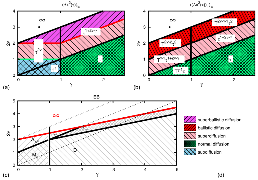
Figure 14: Phase diagram for the ensemble-averaged squared displacement (a), the ensemble average of the time-averaged squared displacement (b), and the ergodicity breaking parameter (c). Different ranges of validity of the analytical results are separated by thick black lines in the two-dimensional parameter space. Different kinds of diffusion are color-coded as indicated in the key. The dotted lines in (c) serve as a guide to the eye for a better comparison with the phase diagram in (b). The ergodicity breaking parameter EB is defined as variance of the rescaled random variable EB$=<\hat{\xi}^{2}(\tau)>_{E}-1$, where $<\hat{\xi}(\tau)>=<\Delta x^{2}(\tau)>_{T}/<<\Delta x^{2}(\tau)>_{T}>_{E}$ with subscripts refering to time (T) and ensemble (E) averages. Adapted from Albers and Radons Albers2018 . With permission from PRL.

V Conclusions

In this work, we discussed some major achievements in the formulation and evolution of the FDT. The breakthrough works of Einstein, Smoluchowski and Langevin established a simple and linear relation between the fluctuation and the dissipation in a physical system.

Moreover, within the approach the standard deviation appears as a very important source of information. Two basic examples of fluctuation phenomena - diffusion and random growth - were discussed along these lines. Both of them have a powerful impact in physics and brought a large number of applications outside physical science. A few years after the origins of quantum mechanics, also the quantum fluctuations-dissipation theorems were born and with them a new physics emerged.

The revolutionary use of the fluctuation-dissipation formalism in various domains of science continues and has gained new strength in the last two decades. One recent example was the use of the growth fluctuation-dissipation theorem GomesFilho21 to obtain the KPZ exponents GomesFilho21b .

Every day we are surprised by new and exciting discoveries within the scope of quantum thermodynamics Funo18 ; Sampaio18 ; Shibata20 ; Bull20 ; Hsiang20 , and it is quite certain that it will continue for the next years to come.

Conflict of Interest Statement

The authors declare that the research was conducted in the absence of any commercial or financial relationships that could be construed as a potential conflict of interest.

Author Contributions

All authors wrote sections of the manuscript. All authors contributed to manuscript revision, read, and approved the submitted version.

Funding

This work was supported by the Conselho Nacional de Desenvolvimento Científico e Tecnológico (CNPq), Grant No. CNPq-303119/2022-5, Fundação de Apoio a Pesquisa do Rio de Janeiro (FAPERJ), Grant No. E-26/203953/2022 (F.A.O.), E.G.N. acknowledges financial support by the Priority Research Area DigiWorld under the program Excellence Initiative - Research University at the Jagiellonian University in Kraków. M.S.G.F acknowledge financial support from grant number #2023/03658-9, São Paulo Research Foundation (FAPESP).

References

- (1) Brown, R. A brief account of microscopical observations made in the months on June, July, and August, 1827, on the particles contained in the pollen of plants; and on the general existence of active molecules in organic and inorganic bodies. Phil. Mag. 4, 161 (1828).
- (2) Brown, R. Mikroskopische beobachtungen über die im pollen der pflanzen enthaltenen partikeln, und über das allgemeine vorkommen activer molecüle in organischen und unorganischen körpern. Ann. Phys. Chem. B 14, 294 (1828).
- (3) Langevin, P. Sur la theorie du mouvement Brownien. Comptes Rendus 146, 530 (1908).
- (4) Nyquist, H. Thermal agitation of electric charge in conductors. Physical Review 32, 110 (1928).
- (5) Johnson, J. B. Thermal agitation of electricity in conductors. Physical Review 32, 97 (1928).
- (6) Onsager, L. Reciprocal relations in irreversible processes I. Phys. Rev. 37, 405 (1931).
- (7) Callen, H. B. & Welton, T. A. Irreversibility and generalized noise. Phys. Rev. 83, 34–40 (1951). URL https://link.aps.org/doi/10.1103/PhysRev.83.34.
- (8) Callen, H. B. & Greene, R. F. On a theorem of irreversible thermodynamics. Phys. Rev. 86, 702 (1952).
- (9) Jülicher, F., Ajdari, A. & Prost, J. Modeling molecular motors. Reviews of Modern Physics 69, 1269 (1997).
- (10) Astumian, R. D. & Bier, M. Fluctuation driven ratchets: molecular motors. Physical Review Letters 72, 1766 (1994).
- (11) Schliwa, M. & Woehlke, G. Molecular motors. Nature 422, 759–765 (2003).
- (12) Baroncini, M., Silvi, S. & Credi, A. Photo-and redox-driven artificial molecular motors. Chemical Reviews 120, 200–268 (2019).
- (13) Chowdhury, D. Stochastic mechano-chemical kinetics of molecular motors: A multidisciplinary enterprise from a physicist’s perspective. Physics Reports 529, 1–197 (2013).
- (14) Astumian, R. D. & Bier, M. Mechanochemical coupling of the motion of molecular motors to ATP hydrolysis. Biophysical Journal 70, 637–653 (1996).
- (15) Hoffmann, P. M. How molecular motors extract order from chaos (a key issues review). Reports on Progress in Physics 79, 032601 (2016).
- (16) Bao, J.-D. & Zhuo, Y.-Z. Ballistic diffusion induced by a thermal broadband noise. Phys. Rev. Lett. 91, 138104 (2003). URL https://link.aps.org/doi/10.1103/PhysRevLett.91.138104.
- (17) Bao, J. D., Zhuo, Y. Z., Oliveira, F. A. & Hänggi, P. Intermediate dynamics between Newton and Langevin. Phys. Rev. E 74, 061111 (2006). URL http://link.aps.org/abstract/PRE/v74/e061111.
- (18) Nettesheim, G. et al. Macromolecular crowding acts as a physical regulator of intracellular transport. Nature Physics 1–8 (2020).
- (19) Conca, C., Diaz, J. I., Linan, A. & Timofte, C. Homogenization in chemical reactive flows. Electronic Journal of Differential Equations (EJDE)[electronic only] 40, 1–22 (2004).
- (20) Gammaitoni, L., Hänggi, P., Jung, P. & Marchesoni, F. Stochastic resonance. Reviews of Modern Physics 70, 223 (1998).
- (21) Benzi, R., Sutera, A. & Vulpiani, A. The mechanism of stochastic resonance. Journal of Physics A: Mathematical and General 14, L453 (1981).
- (22) Barabási, A. L. & Stanley, H. E. Fractal Concepts in Surface Growth (Cambridge University Press, Cambridge, 1995).
- (23) Edwards, S. F. & Wilkinson, D. R. The surface statistics of a granular aggregate. Proc. R. Soc. Lond. A 381, 17–31 (1982).
- (24) Kardar, M., Parisi, G. & Zhang, Y.-C. Dynamic scaling of growing interfaces. Phys. Rev. Lett. 56, 889–892 (1986). URL http://link.aps.org/doi/10.1103/PhysRevLett.56.889.
- (25) Gontis, V., Ruseckas, J. & Kononovičius, A. A long-range memory stochastic model of the return in financial markets. Physica A: Statistical Mechanics and its Applications 389, 100–106 (2010).
- (26) Urry, J. Small worlds and the new ‘social physics’. Global networks 4, 109–130 (2004).
- (27) Chekroun, M. D., Simonnet, E. & Ghil, M. Stochastic climate dynamics: Random attractors and time-dependent invariant measures. Physica D: Nonlinear Phenomena 240, 1685–1700 (2011).
- (28) Image from sarah richter by pixabay. https://pixabay.com/pt/photos/tinta-%C3%A1gua-copo-de-%C3%A1gua-l%C3%ADquido-2427263/ (Accessed: May 29, 2020).
- (29) Free-photos by pixabay. https://pixabay.com/pt/photos/neve-rua-moradias-em-banda-cidade-1030928/ (Accessed: May 29, 2020).
- (30) Kubo, R., Toda, M. & Hashitsume, N. Statistical Physics II (Springer, Berlin, 1991).
- (31) Gauss, C. Theoria Motus Corporum Coelestium in Sectionibus Conicis Solum Ambientium (English Translation by Dover Publications, Mineola, 1857).
- (32) Laplace, P. Théorie Analytique de Probabilites (V. Courcier, Paris, 1812).
- (33) Salinas, S. Introduction to Statistical Physics (Springer, New York, 2001).
- (34) Huang, K. Statistical Mechanics (John Wiley & Sons, New york, 1987).
- (35) Falk, H. & Bruch, L. W. Susceptibility and fluctuation. Physical Review 180, 442 (1969).
- (36) Pinto, P. D., Oliveira, F. A. & Penna, A. L. A. Thermodynamics aspects of noise-induced phase synchronization. Phys. Rev. E 93, 052220 (2016). URL https://link.aps.org/doi/10.1103/PhysRevE.93.052220.
- (37) Pinto, P. D., Penna, A. L. & Oliveira, F. A. Critical behavior of noise-induced phase synchronization. EPL (Europhysics Letters) 117, 50009 (2017).
- (38) Paul, W. & Baschnagel, J. Stochastic processes, vol. 1 (Springer, 2013).
- (39) Morgado, R., Oliveira, F. A., Batrouni, G. G. & Hansen, A. Relation between anomalous and normal diffusion in systems with memory. Phys. Rev. Lett. 89, 100601 (2002).
- (40) Costa, I. V. L., Morgado, R., Lima, M. V. B. T. & Oliveira, F. A. The fluctuation-dissipation theorem fails for fast superdiffusion. Europhys. Lett. 63, 173 (2003).
- (41) Metzler, R., Barkai, E. & Klafter, J. Anomalous diffusion and relaxation close to thermal equilibrium: A fractional Fokker-Planck equation approach. Phys. Rev. Lett. 82, 3563 (1999).
- (42) Sancho, J. M., Lacasta, A. M., Lindenberg, K., Sokolov, I. M. & Romero, A. H. Diffusion on a solid surface: Anomalous is normal. Phys. Rev. Lett. 92, 250601 (2004). URL https://link.aps.org/doi/10.1103/PhysRevLett.92.250601.
- (43) Lapas, L. C., Costa, I. V. L., Vainstein, M. H. & Oliveira, F. A. Entropy, non-ergodicity and non-gaussian behaviour in ballistic transport. Europhys. Lett. 77, 37004 (2007).
- (44) Lapas, L. C., Morgado, R., Vainstein, M. H., Rubí, J. M. & Oliveira, F. A. Khinchin theorem and anomalous diffusion. Phys. Rev. Lett. 101, 230602 (2008).
- (45) Weron, A. & Magdziarz, M. Generalization of the Khinchin theorem to Lévy flights. Phys. Rev. Lett. 105, 260603 (2010).
- (46) Thiel, F., Flegel, F. & Sokolov, I. M. Disentangling sources of anomalous diffusion. Phys. Rev. Lett. 111, 010601 (2013). URL https://link.aps.org/doi/10.1103/PhysRevLett.111.010601.
- (47) Dorea, C. C. Y. & Medino, A. V. Anomalous diffusion index for Lévy motions. J. Stat. Phys. 123, 685 (2006).
- (48) McKinley, S. A. & Nguyen, H. D. Anomalous diffusion and the generalized Langevin equation. SIAM Journal on Mathematical Analysis 50, 5119–5160 (2018).
- (49) Flekkøy, E. G. Minimal model for anomalous diffusion. Phys. Rev. E 95, 012139 (2017). URL https://link.aps.org/doi/10.1103/PhysRevE.95.012139.
- (50) Vainstein, M. H., Costa, I. V. L. & Oliveira, F. A. Mixing, ergodicity and the fluctuation-dissipation theorem in complex systems. In Miguel, M. C. & Rubí, M. (eds.) Jamming, Yielding, and Irreversible Deformation in Condensed Matter, vol. 688 of Lecture Notes in Phys., 159–188 (Springer Berlin / Heidelberg, 2006).
- (51) dos Santos, M. A. Analytic approaches of the anomalous diffusion: A review. Chaos, Solitons & Fractals 124, 86–96 (2019).
- (52) Metzler, R. & Klafter, J. The random walk’s guide to anomalous diffusion: a fractional dynamics approach. Phys. Rep. 339, 1 (2000).
- (53) Metzler, R. & Klafter, J. The restaurant at the end of the random walk: recent developments in the description of anomalous transport by fractional dynamics. J. Phys. A: Math. Gen. 37, 161 (2004).
- (54) Oliveira, F. A., Ferreira, R. M. S., Lapas, L. C. & Vainstein, M. H. Anomalous diffusion: A basic mechanism for the evolution of inhomogeneous systems. Frontiers in Physics 7, 18 (2019).
- (55) Einstein, A. Über die von der molekularkinetischen theorie der wärme geforderte bewegung von in ruhenden flüssigkeiten suspendierten teilchen. Ann. Phys. 17, 549 (1905).
- (56) Einstein, A. Investigations on the theory of the Brownian Movement (Dover, New York, 1956).
- (57) Gudowska-Nowak, E., Lindenberg, K. & Metzler, R. Preface: Marian Smoluchowski’s 1916 paper—a century of inspiration. J. Phys. A 50, 380301 (2017). URL http://stacks.iop.org/1751-8121/50/i=38/a=380301.
- (58) Oliveira, F. A. & Taylor, P. L. Breaking in polymer chains. II. The Lennard‐Jones chain. J. Chem. Phys. 101, 10118–10125 (1994). URL http://dx.doi.org/10.1063/1.468000. eprint http://dx.doi.org/10.1063/1.468000.
- (59) Oliveira, F. A. Dynamical renormalization of anharmonic lattices at the onset of fracture: Analytical results for scaling, noise, and memory. Phys. Rev. B 52, 1009 (1995).
- (60) Oliveira, F. A., Mello, B. A. & Xavier, I. M. Scaling transformation of random walk distributions in a lattice. Phys. Rev. E 61, 7200 (2000).
- (61) Lévy, P. Théorie de l’Addition des Variables Aléatoires (Guthier-Villars, Paris, 1954).
- (62) Leite, R. C., Moore, R. S. & Porto, S. P. Use of a gas laser in studies of the depolarization of the Rayleigh scattering from simple liquids. The Journal of Chemical Physics 40, 3741–3742 (1964).
- (63) Penna, A., Chaves, A., Andrade, P. d. R. & Porto, S. P. Light scattering by lithium tantalate at room temperature. Physical Review B 13, 4907 (1976).
- (64) Marcus, R. A. Exchange reactions and electron transfer reactions including isotopic exchange. theory of oxidation-reduction reactions involving electron transfer. part 4.—a statistical-mechanical basis for treating contributions from solvent, ligands, and inert salt. Discussions of the Faraday Society 29, 21–31 (1960).
- (65) Oliveira, F. A. Time-reversal symmetry in light scattering by excitations in a film. Solid State Commun. 40, 859–861 (1981).
- (66) Loudon, R. The Quantum Theory of Light (Oxford University Press, New York, 2000).
- (67) Santos, M. B. L., Oliveira, E. A. & Neto, A. M. F. Rayleigh scattering of a new lyotropic nematic liquid crystal system: crossover of propagative and diffusive behavior. Liq. Cryst. 27, 1485 (2000).
- (68) Benmouna, F. et al. Dynamic light scattering from liquid crystal polymer brushes swollen in a nematic solvent. Liq. Cryst. 28, 1353 (2001).
- (69) Oliveira, F., Cottam, M. & Tilley, D. Green functions, power spectra, and raman scattering of thin film polaritons. Physica Status Solidi (b) 107, 737–747 (1981).
- (70) Rahman, A., Singwi, K. S. & Sjölander, A. Stochastic model of a liquid and cold neutron scattering. II. Phys. Rev. 126, 997–1004 (1962). URL https://link.aps.org/doi/10.1103/PhysRev.126.997.
- (71) Yulmetyev, R. M., Mokshin, A. V. & Hänggi, P. Diffusion time-scale invariance, randomization processes, and memory effects in Lennard-Jones liquids. Phys. Rev. E 68, 051201 (2003). URL https://link.aps.org/doi/10.1103/PhysRevE.68.051201.
- (72) Florencio, J. & Lee, M. H. Exact time evolution of a classical harmonic-oscilator chain. Phys. Rev. A 31, 3231 (1985).
- (73) Odell, J. A. & Taylor, M. A. Dynamics and thermomechanical stability of DNA in solution. Biopolymers 34, 1483 (1994).
- (74) Toussaint, R., Helgesen, G. & Flekkøy, E. G. Dynamic roughening and fluctuations of dipolar chains. Phys. Rev. Lett. 93, 108304 (2004).
- (75) Doerr, T. P. & Taylor, P. L. Breaking in polymer chains. i. the harmonic chain. The Journal of Chemical Physics 101, 10107–10117 (1994).
- (76) Oliveira, F. A. & Gonzalez, J. A. Bond-stability criterion in chain dynamics. Phys. Rev. B 54, 3954–3958 (1996). URL https://link.aps.org/doi/10.1103/PhysRevB.54.3954.
- (77) Oliveira, F. A. Transition-state analysis for fracture nucleation in polymers: The Lennard-Jones chain. Phys. Rev. B 57, 10576–10582 (1998).
- (78) Gonzalez, J. A. & Oliveira, F. A. Nucleation theory, the escaping processes, and nonlinear stability. Phys. Rev. B 59, 6100 (1999).
- (79) Maroja, A. M., Oliveira, F. A., Cieśla, M. & Longa, L. Polymer fragmentation in extensional flow. Phys. Rev. E 63, 061801 (2001). URL https://link.aps.org/doi/10.1103/PhysRevE.63.061801.
- (80) Dias, C. L., Dubé, M., Oliveira, F. A. & Grant, M. Scaling in force spectroscopy of macromolecules. Phys. Rev. E 72, 011918 (2005). URL https://link.aps.org/doi/10.1103/PhysRevE.72.011918.
- (81) Sain, A., Dias, C. L. & Grant, M. Rupture of an extended object: A many-body Kramers calculation. Phys. Rev. E 74, 046111 (2006). URL https://link.aps.org/doi/10.1103/PhysRevE.74.046111.
- (82) Azevedo, D., da Silva, K. A., Mauriz, P., Viswanathan, G. & Oliveira, F. Fractal behavior of poly (GC) and poly (TA) DNA segments arranged in quasiperiodic fibonacci sequence. Physica A: Statistical Mechanics and its Applications 445, 27–34 (2016).
- (83) Bao, J.-D. Transport in a flashing ratchet in the presence of anomalous diffusion. Phys. Lett. A 314, 203 – 208 (2003). URL http://www.sciencedirect.com/science/article/pii/S0375960103009101.
- (84) Qiu, Q., Shi, X.-Y. & Bao, J.-D. Mixed nonergodicity of a forced system and its non-stationary strength. EPL (Europhysics Letters) 128, 20005 (2019).
- (85) Dyre, J. C. & Schrøder, T. B. Universality of AC conduction in disordered solids. Rev. Mod. Phys. 72, 873–892 (2000). URL https://link.aps.org/doi/10.1103/RevModPhys.72.873.
- (86) Oliveira, F. A., Morgado, R., Hansen, A. & Rubí, J. M. Superdiffusive conduction: AC conductivity with correlated noise. Physica A 357, 115–121 (2005).
- (87) Kramers, H. A. Brownian motion in a field of force and the diffusion model of chemical reactions. Physica 7, 284 (1940).
- (88) Oliveira, F. A. Reaction rate theory for non-Markovian systems. Physica A 257, 128 (1998).
- (89) Hänggi, P. & Thomas, H. Time evolution, correlations, and linear response of non-Markov processes. Z. Physik B 26, 85 (1977).
- (90) Hänggi, P., Talkner, P. & Borkovec, M. Reaction-rate theory: fifty years after Kramers. Rev. Mod. Phys. 62, 251–341 (1990). URL https://link.aps.org/doi/10.1103/RevModPhys.62.251.
- (91) Boccaletti, S., Kurths, J., Osipov, G., Valladares, D. L. & Zhou, C. S. The synchronization of chaotic systems. Phys. Rep. 366, 1–101 (2002).
- (92) Longa, L., Curado, E. M. F. & Oliveira, F. A. Roundoff-induced coalescence of chaotic trajectories. Phys. Rev. E 54, R2201 (1996).
- (93) Maritan, A. & Banavar, J. R. Chaos, noise, and synchronization. Physical Review Letters 72, 1451 (1994).
- (94) Cieśla, M., Dias, S. P., Longa, L. & Oliveira, F. A. Synchronization induced by Langevin dynamics. Phys. Rev. E 63, 065202 (2001). URL https://link.aps.org/doi/10.1103/PhysRevE.63.065202.
- (95) Osipov, G. V., Kurths, J. & Zhou, C. Synchronization in oscillatory networks (Springer Science & Business Media, 2007).
- (96) Morgado, R., Cieśla, M., Longa, L. & Oliveira, F. A. Synchronization in the presence of memory. Europhys. Lett. 79, 10002 (2007).
- (97) Siepmann, J. & Siepmann, F. Modeling of diffusion controlled drug delivery. Journal of Controlled Release 161, 351 – 362 (2012). Drug Delivery Research in Europe.
- (98) Gomes Filho, M. S., Oliveira, F. A. & Barbosa, M. A. A. A statistical mechanical model for drug release: Investigations on size and porosity dependence. Physica A 460, 29–37 (2016).
- (99) Ignacio, M., Chubynsky, M. V. & Slater, G. W. Interpreting the Weibull fitting parameters for diffusion-controlled release data. Physica A 486, 486–496 (2017).
- (100) Singh, K., Satapathi, S. & Jha, P. K. “Ant-wall” model to study drug release from excipient matrix. Physica A: Statistical Mechanics and its Applications 519, 98 – 108 (2019).
- (101) Mircioiu, C. et al. Mathematical modeling of release kinetics from supramolecular drug delivery systems. Pharmaceutics 11, 140 (2019).
- (102) Gomes-Filho, M. S., Barbosa, M. A. A. & Oliveira, F. A. A statistical mechanical model for drug release: Relations between release parameters and porosity. Physica A: Statistical Mechanics and its Applications 540, 123165 (2020).
- (103) Yang, Y. et al. E-jet 3d printed drug delivery implants to inhibit growth and metastasis of orthotopic breast cancer. Biomaterials 230, 119618 (2020).
- (104) Gomes-Filho, M. S., Oliveira, F. A. & Barbosa, M. A. A. Modeling the diffusion-erosion crossover dynamics in drug release. Phys. Rev. E 105, 044110 (2022). URL https://link.aps.org/doi/10.1103/PhysRevE.105.044110.
- (105) Vainstein, M. H., Lapas, L. C. & Oliveira, F. A. Anomalous diffusion. Acta Physica Polonica B 39 (2008).
- (106) Donato, C., Oliveira, F. & Gomes, M. Anomalous diffusion on crumpled wires in two dimensions. Physica A: Statistical Mechanics and its Applications 368, 1 – 6 (2006).
- (107) Banks, R. Growth and Diffusion Phenomena: Mathematical Frameworks and Applications (Springer-Verlag Berlin, 1994).
- (108) Murray, J. D. Mathematical Biology I. An Introduction, vol. 17 of Interdisciplinary Applied Mathematics (Springer, New York, 2002), 3 edn.
- (109) Fisher, R. A. The wave of advance of advantageous genes. Annals of Eugenics 7, 355–369 (1937).
- (110) Rothe, F. Global solutions of reaction-diffusion systems (Lecture Notes in Mathematics 1072, Springer-Verlag Berlin Heidelberg, 1984).
- (111) Aranda, O. T. & Oliveira, F. A. Analytical and numerical solutions of the riccati equation using the method of variation of parameters. application to population dynamics. Journal of Computational and Nonlinear Dynamics (2020).
- (112) Aranda, O. T., Penna, A. L. & Oliveira, F. A. Nonlinear self-organized population dynamics induced by external selective nonlocal processes. Communications in Nonlinear Science and Numerical Simulation 93, 105512 (2021).
- (113) Aranda, O. T., Penna, A. L. & Oliveira, F. A. Nonlocal pattern formation effects in evolutionary population dynamics. Physica A: Statistical Mechanics and its Applications 572, 125865 (2021). URL https://www.sciencedirect.com/science/article/pii/S0378437121001370.
- (114) Landau, L. D. Collected papers of LD Landau (Pergamon, 1965).
- (115) Cross, M. C. & Hohenberg, P. C. Pattern formation outside of equilibrium. Rev. Mod. Phys. 65, 851–1112 (1993).
- (116) Turing, A. M. The chemical basis of morphogenesis. Philosophical Transactions of the Royal Society of London. Series B, Biological Sciences 237, 37–72 (1952).
- (117) Kolmogorov, A. N. A study of the equation of diffusion with increase in the quantity of matter, and its application to a biological problem. Moscow University Bulletin of Mathematics 1, 1–25 (1937).
- (118) da Cunha, J. A., Penna, A. L. & Oliveira, F. A. Pattern formation and coexistence domains for a nonlocal population dynamics. Physical Review E 83, 015201 (2011).
- (119) Koch, A. & Meinhardt, H. Biological pattern formation: from basic mechanisms to complex structures. Reviews of Modern Physics 66, 1481 (1994).
- (120) Nicolis, G. & Nicolis, G. Introduction to nonlinear science (Cambridge university press, 1995).
- (121) Newel, A. C. Pattern Formation in the Physical and Biological Sciences (Santa Fe Institute Studies in the Sciences of Complexity, Lecture Notes Vol 5) (Ch. The Dynamics and Analysis of Patterns, 1997).
- (122) Rabinovich, M. I., Ezersky, A. B. & Weidman, P. D. The dynamics of patterns (World Scientific, 2000).
- (123) Fuentes, M., Kuperman, M. & Kenkre, V. Nonlocal interaction effects on pattern formation in population dynamics. Physical Review Letters 91, 158104 (2003).
- (124) Fuentes, M., Kuperman, M. & Kenkre, V. Analytical considerations in the study of spatial patterns arising from nonlocal interaction effects. The Journal of Physical Chemistry B 108, 10505–10508 (2004).
- (125) Da Cunha, J., Penna, A., Vainstein, M., Morgado, R. & Oliveira, F. Self-organization analysis for a nonlocal convective fisher equation. Physics Letters A 373, 661–667 (2009).
- (126) Colombo, E. H. & Anteneodo, C. Nonlinear diffusion effects on biological population spatial patterns. Physical Review E 86, 036215 (2012).
- (127) Barbosa, F. V. et al. Pattern transitions and complexity for a nonlocal logistic map. Physica A: Statistical Mechanics and its Applications 473, 301–312 (2017).
- (128) Fusco, D., Gralka, M., Kayser, J., Anderson, A. & Hallatschek, O. Excess of mutational jackpot events in expanding populations revealed by spatial Luria–Delbrück experiments. Nat. Commun. 7, 12760 (2016).
- (129) Almeida, R. A. L., Ferreira, S. O., Oliveira, T. J. & Aarão Reis, F. D. A. Universal fluctuations in the growth of semiconductor thin films. Phys. Rev. B 89, 045309 (2014).
- (130) Mello, B. A., Chaves, A. S. & Oliveira, F. A. Discrete atomistic model to simulate etching of a crystalline solid. Phys. Rev. E 63, 041113 (2001). URL http://link.aps.org/doi/10.1103/PhysRevE.63.041113.
- (131) Gomes, W. P., Penna, A. L. A. & Oliveira, F. A. From cellular automata to growth dynamics: The Kardar-Parisi-Zhang universality class. Phys. Rev. E 100, 020101 (2019). URL https://link.aps.org/doi/10.1103/PhysRevE.100.020101.
- (132) Merikoski, J., Maunuksela, J., Myllys, M., Timonen, J. & Alava, M. J. Temporal and spatial persistence of combustion fronts in paper. Phys. Rev. Lett. 90, 24501 (2003).
- (133) Hansen, A., Schmittbuhl, J., Batrouni, G. G. & de Oliveira, F. A. Normal stress distribution of rough surfaces in contact. Geophys. Res. Lett. 27, 3639–3642 (2000).
- (134) Forster, D., Nelson, D. R. & Stephen, M. J. Large-distance and long-time properties of a randomly stirred fluid. Phys. Rev. A 16, 732–749 (1977). URL https://link.aps.org/doi/10.1103/PhysRevA.16.732.
- (135) Ódor, G., Liedke, B. & Heinig, K.-H. Directed -mer diffusion describing the Kardar-Parisi-Zhang-type surface growth. Phys. Rev. E 81, 031112 (2010).
- (136) Takeuchi, K. A. Crossover from growing to stationary interfaces in the Kardar-Parisi-Zhang class. Phys. Rev. Lett. 110, 210604 (2013).
- (137) Almeida, R. A. L., Ferreira, S. O., Ferraz, I. & Oliveira, T. J. Initial pseudo-steady state & asymptotic KPZ universality in semiconductor on polymer deposition. Sci. Rep. 7, 3773 (2017).
- (138) Aarão Reis, F. D. A. Numerical study of roughness distributions in nonlinear models of interface growth. Phys. Rev. E 72, 032601 (2005). URL http://link.aps.org/doi/10.1103/PhysRevE.72.032601.
- (139) Rodrigues, E. A., Mello, B. A. & Oliveira, F. A. Growth exponents of the etching model in high dimensions. J. Phys. A 48, 35001–35012 (2015).
- (140) Alves, W. S. et al. Analysis of etching at a solid-solid interface. Phys. Rev. E 94, 042119 (2016).
- (141) Carrasco, I. S. S. & Oliveira, T. J. Kardar-Parisi-Zhang growth on one-dimensional decreasing substrates. Phys. Rev. E 98, 010102 (2018).
- (142) Krug, J., Meakin, P. & Halpin-Healy, T. Amplitude universality for driven interfaces and directed polymers in random media. Physical Review A 45, 638 (1992).
- (143) Krug, J. Origins of scale invariance in growth processes. Adv. Phys. 46, 139–282 (1997).
- (144) Derrida, B. & Lebowitz, J. L. Exact large deviation function in the asymmetric exclusion process. Physical Review Letters 80, 209 (1998).
- (145) Meakin, P., Ramanlal, P., Sander, L. M. & Ball, R. Ballistic deposition on surfaces. Physical Review A 34, 5091 (1986).
- (146) Daryaei, E. Universality and crossover behavior of single-step growth models in 1+ 1 and 2+ 1 dimensions. Physical Review E 101, 062108 (2020).
- (147) Gwa, L.-H. & Spohn, H. Six-vertex model, roughened surfaces, and an asymmetric spin hamiltonian. Physical Review Letters 68, 725 (1992).
- (148) De Vega, H. & Woynarovich, F. Method for calculating finite size corrections in bethe ansatz systems: Heisenberg chain and six-vertex model. Nuclear Physics B 251, 439–456 (1985).
- (149) Plischke, M., Rácz, Z. & Liu, D. Time-reversal invariance and universality of two-dimensional growth models. Physical Review B 35, 3485 (1987).
- (150) Corwin, I., Ghosal, P., Krajenbrink, A., Le Doussal, P. & Tsai, L.-C. Coulomb-gas electrostatics controls large fluctuations of the Kardar-Parisi-Zhang equation. Physical Review Letters 121, 060201 (2018).
- (151) Nahum, A., Ruhman, J., Vijay, S. & Haah, J. Quantum entanglement growth under random unitary dynamics. Physical Review X 7, 031016 (2017).
- (152) Ljubotina, M., Žnidarič, M. & Prosen, T. Kardar-Parisi-Zhang physics in the quantum Heisenberg magnet. Physical Review Letters 122, 210602 (2019).
- (153) De Nardis, J., Medenjak, M., Karrasch, C. & Ilievski, E. Anomalous spin diffusion in one-dimensional antiferromagnets. Phys. Rev. Lett. 123, 186601 (2019).
- (154) Vainstein, M. H., Morgado, R., Oliveira, F. A., de Moura, F. A. B. F. & Coutinho-Filho, M. D. Stochastic description of the dynamics of the random-exchange Heisenberg chain. Phys. Lett. A 339, 33–38 (2005).
- (155) Prykarpatski, A. K., Pukach, P. Y. & Vovk, M. I. Symplectic geometry aspects of the parametrically-dependent Kardar–Parisi–Zhang equation of spin glasses theory, its integrability and related thermodynamic stability. Entropy 25, 308 (2023).
- (156) Dasgupta, C., Sarma, S. D. & Kim, J. Controlled instability and multiscaling in models of epitaxial growth. Physical Review E 54, R4552 (1996).
- (157) Dasgupta, C., Kim, J., Dutta, M. & Sarma, S. D. Instability, intermittency, and multiscaling in discrete growth models of kinetic roughening. Physical Review E 55, 2235 (1997).
- (158) Torres, M. & Buceta, R. Numerical integration of KPZ equation with restrictions. Journal of Statistical Mechanics: Theory and Experiment 2018, 033208 (2018).
- (159) Wio, H. S., Revelli, J. A., Deza, R. R., Escudero, C. & de la Lama, M. S. KPZ equation: Galilean-invariance violation, consistency, and fluctuation-dissipation issues in real-space discretization. EPL (Europhysics Letters) 89, 40008 (2010).
- (160) Wio, H. S. et al. d-dimensional KPZ equation as a stochastic gradient flow in an evolving landscape: Interpretation and time evolution of its generating functional. Frontiers in Physics 4, 52 (2017).
- (161) Rodríguez, M. A. & Wio, H. S. Stochastic entropies and fluctuation theorems for a discrete one-dimensional kardar-parisi-zhang system. Physical Review E 100, 032111 (2019).
- (162) Bertini, L. & Giacomin, G. Stochastic Burgers and KPZ equations from particle systems. Commun. Math. Phys. 183, 571–607 (1997).
- (163) Baik, J., Deift, P. & Johansson, K. On the distribution of the length of the longest increasing subsequence of random permutations. Journal of the American Mathematical Society 12, 1119–1178 (1999).
- (164) Prähofer, M. & Spohn, H. Universal distributions for growth processes in dimensions and random matrices. Phys. Rev. Lett. 84, 4882–4885 (2000). URL https://link.aps.org/doi/10.1103/PhysRevLett.84.4882.
- (165) Dotsenko, V. Replica Bethe ansatz derivation of the Tracy–Widom distribution of the free energy fluctuations in one-dimensional directed polymers. Journal of Statistical Mechanics: Theory and Experiment 2010, P07010 (2010).
- (166) Calabrese, P., Le Doussal, P. & Rosso, A. Free-energy distribution of the directed polymer at high temperature. EPL (Europhysics Letters) 90, 20002 (2010).
- (167) Amir, G., Corwin, I. & Quastel, J. Probability distribution of the free energy of the continuum directed random polymer in 1+ 1 dimensions. Communications on Pure and Applied mathematics 64, 466–537 (2011).
- (168) Sasamoto, T. & Spohn, H. One-dimensional Kardar-Parisi-Zhang equation: An exact solution and its universality. Phys. Rev. Lett. 104, 230602 (2010). URL http://dx.doi.org/10.1103/PhysRevLett.104.230602.
- (169) Le Doussal, P., Majumdar, S. N., Rosso, A. & Schehr, G. Exact short-time height distribution in the one-dimensional Kardar-Parisi-Zhang equation and edge fermions at high temperature. Phys. Rev. Lett. 117, 070403 (2016).
- (170) Hairer, M. Solving the KPZ equation. Ann. Math. 178, 559–664 (2013). URL http://annals.math.princeton.edu/2013/178-2/p04.
- (171) Johansson, K. Shape fluctuations and random matrices. Commun. Math. Phys. 209, 437–476 (2000).
- (172) Gomes-Filho, M. S., Penna, A. L. & Oliveira, F. A. The Kardar-Parisi-Zhang exponents for the 2+1 dimensions. Results in Physics 26, 104435 (2021).
- (173) Mello, B. A. A random rule model of surface growth. Physica A 419, 762–767 (2015).
- (174) Kriecherbauer, T. & Krug, J. A pedestrian’s view on interacting particle systems, KPZ universality and random matrices. Journal of Physics A: Mathematical and Theoretical 43, 403001 (2010). URL https://doi.org/10.1088%2F1751-8113%2F43%2F40%2F403001.
- (175) Halpin-Healy, T. & Takeuchi, K. A. A KPZ cocktail-shaken, not stirred… Journal of Statistical Physics 160, 794–814 (2015).
- (176) Carrasco, I. S. S., Takeuchi, K. A., Ferreira, S. C. & Oliveira, T. J. Interface fluctuations for deposition on enlarging flat substrates. New Journal of Physics 16, 123057 (2014).
- (177) Fukai, Y. T. & Takeuchi, K. A. Kardar-Parisi-Zhang interfaces with inward growth. Phys. Rev. Lett. 119, 030602 (2017).
- (178) Carrasco, I. S. S. & Oliveira, T. J. Circular Kardar-Parisi-Zhang interfaces evolving out of the plane. Phys. Rev. E 99, 032140 (2019). URL https://link.aps.org/doi/10.1103/PhysRevE.99.032140.
- (179) Gomes-Filho, M. S. & Oliveira, F. A. The hidden fluctuation-dissipation theorem for growth. EPL (Europhysics Letters) 133, 10001 (2021).
- (180) dos Anjos, P. H. R., Gomes-Filho, M. S., Alves, W. S., Azevedo, D. L. & Oliveira, F. A. The fractal geometry of growth: Fluctuation–dissipation theorem and hidden symmetry. Frontiers in Physics 9 (2021). URL https://www.frontiersin.org/articles/10.3389/fphy.2021.741590.
- (181) Wolf, D. & Kertesz, J. Surface width exponents for three-and four-dimensional eden growth. Europhys. Lett. 4, 651 (1987).
- (182) Kim, J. M. & Kosterlitz, J. Growth in a restricted solid-on-solid model. Physical review letters 62, 2289 (1989).
- (183) Lässig, M. Quantized scaling of growing surfaces. Phys. Rev. Lett. 80, 2366–2369 (1998). URL https://link.aps.org/doi/10.1103/PhysRevLett.80.2366.
- (184) Sun, T. & Plischke, M. Field-theory renormalization approach to the Kardar-Parisi-Zhang equation. Phys. Rev. E 49, 5046–5057 (1994). URL https://link.aps.org/doi/10.1103/PhysRevE.49.5046.
- (185) Canet, L., Chaté, H., Delamotte, B. & Wschebor, N. Nonperturbative renormalization group for the Kardar-Parisi-Zhang equation. Phys. Rev. Lett. 104, 150601 (2010).
- (186) Canet, L., Chaté, H., Delamotte, B. & Wschebor, N. Nonperturbative renormalization group for the Kardar-Parisi-Zhang equation: General framework and first applications. Phys. Rev. E 84, 061128 (2011).
- (187) Oliveira, T. J. Kardar-Parisi-Zhang universality class in (d+ 1)-dimensions. Physical Review E 106, L062103 (2022).
- (188) Orrillo, P. A. et al. Morphological stabilization and kpz scaling by electrochemically induced co-deposition of nanostructured NiW alloy films. Sci. Rep. 7, 1–12 (2017).
- (189) Ojeda, F., Cuerno, R., Salvarezza, R. & Vázquez, L. Dynamics of rough interfaces in chemical vapor deposition: Experiments and a model for silica films. Phys. Rev. Lett. 84, 3125–3128 (2000). URL https://link.aps.org/doi/10.1103/PhysRevLett.84.3125.
- (190) Luis, E. E. M., de Assis, T. A. & Oliveira, F. A. Unveiling the connection between the global roughness exponent and interface fractal dimension in ew and kpz lattice models. Journal of Statistical Mechanics: Theory and Experiment 2022, 083202 (2022). URL https://dx.doi.org/10.1088/1742-5468/ac7e3f.
- (191) Mozo Luis, E. E., Oliveira, F. A. & de Assis, T. A. Accessibility of the surface fractal dimension during film growth. Phys. Rev. E 107, 034802 (2023). URL https://link.aps.org/doi/10.1103/PhysRevE.107.034802.
- (192) Alves, S. G., Oliveira, T. J. & Ferreira, S. C. Universality of fluctuations in the Kardar-Parisi-Zhang class in high dimensions and its upper critical dimension. Phys. Rev. E 90, 020103 (2014). URL https://link.aps.org/doi/10.1103/PhysRevE.90.020103.
- (193) Ford, G. W., Kac, M. & Mazur, P. Statistical mechanics of assemblies of coupled oscillators. J. Math. Phys. 6, 504 (1965).
- (194) Ford, G. W., Lewis, J. T. & F., O. R. Quantum Langevin equation. Phys. Rev. A 37, 4419 (1988).
- (195) Caldeira, A. O. & Leggett, A. J. Quantum tunnelling in a dissipative system. Ann. Phys. 149, 374–456 (1983).
- (196) van Kampen, N. G. Stochastic processes in physics and chemistry (North-Holland, Amsterdam, 1992).
- (197) van Kampen, N. Derivation of the quantum Langevin equation. Journal of Molecular Liquids 71, 97 (1997).
- (198) Takahashi, H. Generalized theory of thermal fluctuations. Journal of the Physical Society of Japan 7, 439–446 (1952).
- (199) Kubo, R. Statistical-Mechanical Theory of Irreversible Processes. I. General Theory and Simple Applications to Magnetic and Conduction Problems. J. Phys. Soc. Jpn. 12, 570–586 (1957). URL http://dx.doi.org/10.1143/JPSJ.12.570. eprint http://dx.doi.org/10.1143/JPSJ.12.570.
- (200) Kubo, R., Yokota, M. & Nakajima, S. Statistical-Mechanical Theory of Irreversible Processes. II. Response to Thermal Disturbance. J. Phys. Soc. Jpn. 12, 1203–1211 (1957). URL http://dx.doi.org/10.1143/JPSJ.12.1203. eprint http://dx.doi.org/10.1143/JPSJ.12.1203.
- (201) Deker, U. & Haake, F. Fluctuation-dissipation theorems for classical processes. Physical Review A 11, 2043 (1975).
- (202) Kubo, R. Response, relaxation and fluctuation. In Kirczenow, G. & Marro, J. (eds.) Transport Phenomena. Lecture Notes in Phys., vol. 31, 74–124 (Springer-Verlag, Berlin, Heidelberg, 1974).
- (203) Ruelle, D. General linear response formula in statistical mechanics, and the fluctuation-dissipation theorem far from equilibrium. Physics Letters A 245, 220–224 (1998).
- (204) Zwanzig, R. Nonequilibrium Statistical Mechanics (Oxford University Press, New York, 2001).
- (205) Seifert, U. Stochastic thermodynamics, fluctuation theorems and molecular machines. Reports on Progress in Physics 75, 126001 (2012).
- (206) Dybiec, B., Parrondo, J. M. R. & Gudowska-Nowak, E. Fluctuation-dissipation relations under Lévy noises. EPL 98, 50006 (2012). URL http://stacks.iop.org/0295-5075/98/i=5/a=50006.
- (207) Kuśmierz, Ł., Dybiec, B. & Gudowska-Nowak, E. Thermodynamics of superdiffusion generated by Lévy-Wiener fluctuating forces. Entropy 20, 658 (2018).
- (208) Kuśmierz, Ł., Rubi, J. M. & Gudowska-Nowak, E. Heat and work distributions for mixed Cauchy-Gauss process. J. Stat. Mech. Theory and Experiment 2014, P09002 (2014).
- (209) Marconi, U. M. B., Puglisi, A., Rondoni, L. & Vulpiani, A. Fluctuation–dissipation: response theory in statistical physics. Physics Reports 461, 111–195 (2008).
- (210) Sarracino, A. & Vulpiani, A. On the fluctuation-dissipation relation in non-equilibrium and non-hamiltonian systems. Chaos: An Interdisciplinary Journal of Nonlinear Science 29, 083132 (2019).
- (211) Winkler, M. et al. Onsager-symmetry obeyed in athermal mesoscopic systems: Two-phase flow in porous media. arXiv preprint arXiv:2001.04332 (2020).
- (212) Bochkov, G. N. & Kuzovlev, Y. E. General theory of thermal fluctuations in nonlinear systems. Sov. Phys. JETP 45, 125 (1977).
- (213) Bochkov, G. N. & Kuzovlev, Y. E. Nonlinear fluctuation-dissipation relations and stochastic models in nonequilibrium thermodynamics : I. Generalized fluctuation-dissipation theorem. Physica A 106, 443–479 (1981).
- (214) Jarzynski, C. Nonequilibrium equality for free energy differences. Phys. Rev. Lett. 78, 2690–2693 (1997).
- (215) Jarzynski, C. Hamiltonian derivation of a detailed fluctuation theorem. Journal of Statistical Physics 98, 77–102 (2000).
- (216) Crooks, G. E. Entropy production fluctuation theorem and the nonequilibrium work relation for free energy differences. Physical Review E 60, 2721 (1999).
- (217) Saira, O.-P. et al. Test of the Jarzynski and Crooks fluctuation relations in an electronic system. Physical Review Letters 109, 180601 (2012).
- (218) Mori, H. Transport, Collective Motion, and Brownian Motion. Prog. Theor. Phys. 33, 423 (1965).
- (219) Mori, H. A continued-fraction representation of the time-correlation function. Prog. Theor. Phys. 34, 399 (1965).
- (220) Kubo, R. Fluctuation-dissipation theorem. Rep. Prog. Phys. 29, 255 (1966).
- (221) Lee, M. H. Can the velocity autocorrelation function decay exponentially? Phys. Rev. Lett. 51, 1227–1230 (1983).
- (222) Lee, M. H. Solutions of the generalized Langevin equation by a method of recurrence relations. Phys. Rev. B 26, 2547 (1982).
- (223) Lee, M. H. Derivation of the generalized Langevin equation by a method of recurrence relations. J. Math. Phys. 24, 2512 (1983).
- (224) Lee, M. H. & Hong, J. Transport behavior of dense protons in a slab. Phys. Rev. B 30, 6756 (1984).
- (225) Gudowska-Nowak, E., Oliveira, F. A. & Wio, H. S. Editorial: The fluctuation-dissipation theorem today. Frontiers in Physics 10 (2022). URL https://www.frontiersin.org/articles/10.3389/fphy.2022.859799.
- (226) Florêncio, J. & de Alcantara Bonfim, O. F. Recent advances in the calculation of dynamical correlation functions. Frontiers in Physics (2020).
- (227) Chen, L. Y. Application of the brown dynamics fluctuation-dissipation theorem to the study of plasmodium berghei transporter protein pbaqp. Frontiers in Physics 8, 119 (2020).
- (228) Feng, H. & Wang, J. The quantum coherence induced by geometric curvature of gauge field in non-equilibrium quantum dynamics. Frontiers in Physics 8, 129 (2020).
- (229) Reggiani, L. & Alfinito, E. Beyond the formulations of the fluctuation dissipation theorem given by Callen and Welton (1951) and expanded by Kubo (1966). Frontiers in Physics 8, 238 (2020).
- (230) Maes, C. Response theory: A trajectory-based approach. Frontiers in Physics 8, 229 (2020).
- (231) Fotso, H. F. & Freericks, J. K. Characterizing the non-equilibrium dynamics of field-driven correlated quantum systems. Frontiers in Physics 8, 324 (2020).
- (232) Wu, W. & Wang, J. Generalized fluctuation-dissipation theorem for non-equilibrium spatially extended systems. Frontiers in Physics 8, 424 (2020).
- (233) Vainstein, M. H., Costa, I. V. L., Morgado, R. & Oliveira, F. A. Non-exponential relaxation for anomalous diffusion. Europhys. Lett. 73, 726–732 (2006).
- (234) Ferreira, R. M. S., Santos, M. V. S., Donato, C. C., Andrade, J. S. & Oliveira, F. A. Analytical results for long-time behavior in anomalous diffusion. Phys. Rev. E 86, 021121 (2012). URL https://link.aps.org/doi/10.1103/PhysRevE.86.021121.
- (235) Vainstein, M. H., Morgado, R. & Oliveira, F. A. Spatio-temporal conjecture for diffusion. Physica A 357, 109–114 (2005).
- (236) Morgado, R., Costa, I. V. L. & Oliveira, F. A. Normal and anomalous diffusion: Ergodicity and fluctuation-dissipation theorem. Acta Phys. Polon. B 35, 1359 (2004).
- (237) Ferreira, R. M. From generalized Langevin stochastic dynamics to anomalous diffusion. Physical Review E 106, 054157 (2022).
- (238) Srokowski, T. Nonstationarity induced by long-time noise correlations in the langevin equation. Phys. Rev. Lett. 85, 2232 (2000).
- (239) Srokowski, T. Fluctuations in multiplicative systems with jumps. Phys. Rev. E 87, 032104 (2013).
- (240) Joulain, K., Mulet, J.-P., Marquier, F., Carminati, R. & Greffet, J.-J. Surface electromagnetic waves thermally excited: Radiative heat transfer, coherence properties and Casimir forces revisited in the near field. Surface Science Reports 57, 59 – 112 (2005). URL http://www.sciencedirect.com/science/article/pii/S0167572905000105.
- (241) Domingues, G., Volz, S., Joulain, K. & Greffet, J.-J. Heat transfer between two nanoparticles through near field interaction. Phys. Rev. Lett. 94, 085901 (2005). URL https://link.aps.org/doi/10.1103/PhysRevLett.94.085901.
- (242) Pérez-Madrid, A., Rubí, J. M. & Lapas, L. C. Heat transfer between nanoparticles: Thermal conductance for near-field interactions. Phys. Rev. B 77, 155417 (2008). URL https://link.aps.org/doi/10.1103/PhysRevB.77.155417.
- (243) Boltzmann, L. On the development of the methods of theoretical physics in recent times. In Theoretical Physics and Philosophical Problems: Selected Writings (Kluwer Academic Publishers, 1974).
- (244) Khinchin, A. I. Mathematical Foundations of Statistical Mechanics (Dover, New York, 1949).
- (245) Lee, M. H. Why irreversibility is not a sufficient condition for ergodicity. Phys. Rev. Lett. 98, 190601 (2007).
- (246) Lee, M. H. Ergodic theory, infinite products, and long time behavior in hermitian models. Phys. Rev. Lett. 87, 250601 (2001).
- (247) Barrat, A. Monte Carlo simulations of the violation of the fluctuation-dissipation theorem in domain growth processes. Physical Review E 57, 3629 (1998).
- (248) Bellon, L., Buisson, L., Ciccotti, M., Ciliberto, S. & Douarche, F. Thermal noise properties of two aging materials (2005). Cond-mat/0501324.
- (249) Bellon, L. & Ciliberto, S. Experimental study of the fluctuation dissipation relation during an aging process. Physica D: Nonlinear Phenomena 168, 325–335 (2002).
- (250) Crisanti, A. & Ritort, F. Violation of the fluctuation–dissipation theorem in glassy systems: basic notions and the numerical evidence. Journal of Physics A: Mathematical and General 36, R181 (2003).
- (251) Grigera, T. S. & Israeloff, N. E. Observation of fluctuation-dissipation-theorem violations in a structural glass. Phys. Rev. Lett. 83, 5038 (1999).
- (252) Ricci-Tersenghi, F., Stariolo, D. A. & Arenzon, J. J. Two time scales and violation of the fluctuation-dissipation theorem in a finite dimensional model for structural glasses. Phys. Rev. Lett. 84, 4473 (2000).
- (253) Hayashi, K. & Takano, M. Violation of the fluctuation-dissipation theorem in a protein system. Biophysical journal 93, 895–901 (2007).
- (254) Pérez-Madrid, A., Lapas, L. C. & Rubí, J. M. Heat exchange between two interacting nanoparticles beyond the fluctuation-dissipation regime. Phys. Rev. Lett. 103, 048301 (2009). URL https://link.aps.org/doi/10.1103/PhysRevLett.103.048301.
- (255) Averin, D. V. & Pekola, J. P. Violation of the fluctuation-dissipation theorem in time-dependent mesoscopic heat transport. Phys. Rev. Lett. 104, 220601 (2010). URL https://link.aps.org/doi/10.1103/PhysRevLett.104.220601.
- (256) Colaiori, F. & Moore, M. A. Stretched exponential relaxation in the mode-coupling theory for the Kardar-Parisi-Zhang equation. Phys. Rev. E 63, 057103 (2001).
- (257) Rubí, J. M., Santamaría-Holek, I. & Pérez-Madrid, A. Slow dynamics and local quasi-equilibrium - relaxation in supercooled colloidal systems. J. Phys.: Condens. Matter 16, S2047 (2004).
- (258) Peyrard, M. Glass transition in protein hydration water. Phys. Rev. E 64, 011109 (2001).
- (259) Santamaría-Holek, I., Pérez-Madrid, A. & Rubí, J. M. Local quasi-equilibrium description of slow relaxation systems. J. Chem. Phys. 120, 2818 (2004).
- (260) Vainstein, M. H., Stariolo, D. A. & Arenzon, J. J. Heterogeneities in systems with quenched disorder. J. Phys. A: Math. Gen. 36, 10907–10919 (2003).
- (261) Bouchaud, J. P., Mézard, M. & Yedidia, J. S. Variational theory for disordered vortex lattices. Phys. Rev. Lett. 67, 3840 (1991).
- (262) Ferreira, J. L., Ludwig, G. O. & Montes, A. Experimental investigations of ion-acoustic double-layers in the electron flow across multidipole magnetic fields. Plasma Phys. Control. Fusion 33, 297–311 (1991).
- (263) Costa, I. V. L., Vainstein, M. H., Batista, A. A. & Oliveira, F. A. Mixing, ergodicity and slow relaxation phenomena. Physica A 371, 130 (2006).
- (264) Lapas, L. C., Ferreira, R. M., Rubí, J. M. & Oliveira, F. A. Anomalous law of cooling. J. Chem. Phys. 142, 104106 (2015).
- (265) Kohlrausch, R. Theorie des elektrischen rückstandes in der leidener flasche. Ann. Phys 167, 179 (1854).
- (266) Kohlrausch, F. Ueber die elastische nachwirkung bei der torsion. Ann. Phys 195, 337 (1863).
- (267) Mittag-Leffler, G. M. Sur la representation analytique d’une branche uniforme d’une fonction monogene. Acta Math. 29, 101 (1905).
- (268) Stanislavsky, A. & Weron, K. Stochastic tools hidden behind the empirical dielectric relaxation laws. Reports on Progress in Physics 80, 036001 (2017).
- (269) Gudowska-Nowak, E., Bochenek, K., Jurlewicz, A. & Weron, K. Hopping models of charge transfer in a complex environment: Coupled memory continuous-time random walk approach. Phys. Rev. E 72, 061101 (2005). URL https://link.aps.org/doi/10.1103/PhysRevE.72.061101.
- (270) Kuśmierz, Ł., Chechkin, A., Gudowska-Nowak, E. & Bier, M. Breaking microscopic reversibility with Lévy flights. Europhysics Letters 114, 60009 (2016). URL https://dx.doi.org/10.1209/0295-5075/114/60009.
- (271) Kuśmierz, Ł., Ebeling, W., Sokolov, I. & Gudowska-Nowak, E. Onsagers fluctuation theory and new developments including non-equilibrium Lévy fluctuations. Acta Physica Polonica. B 44, 859–887 (2013).
- (272) Ebeling, W., Romanovsky, Y., Sokolov, I. & Valuev, I. Convoluted Gauss-Lévy distributions and exploding Coulomb clusters. Eur.Phys. J. Special Topics 187, 157–170 (2010).
- (273) Sokolov, I., Ebeling, W. & Dybiec, B. Harmonic oscillator under Lévy noise: Unexpected properties in the phase space. Phys. Rev. E 83, 041118 (2011).
- (274) Zaburdaev, V., Denisov, S. & Klafter, J. Lévy walks. Rev. Mod. Phys. 87, 483–530 (2015). URL https://link.aps.org/doi/10.1103/RevModPhys.87.483.
- (275) Albers, T. & Radons, G. Exact results for the nonergodicity of d-dimensional generalized Lévy walks. Phys. Rev. Lett. 120, 104501 (2018).
- (276) Funo, K. & Quan, H. Path integral approach to quantum thermodynamics. Physical Review Letters 121, 040602 (2018).
- (277) Sampaio, R., Suomela, S., Ala-Nissila, T., Anders, J. & Philbin, T. Quantum work in the bohmian framework. Physical Review A 97, 012131 (2018).
- (278) Shibata, N., Yoshioka, N. & Katsura, H. Onsager’s scars in disordered spin chains. Physical Review Letters 124, 180604 (2020).
- (279) Bull, K., Desaules, J.-Y. & Papić, Z. Quantum scars as embeddings of weakly broken Lie algebra representations. Physical Review B 101, 165139 (2020).
- (280) Hsiang, J.-T. & Hu, B.-L. Fluctuation-dissipation relation from the nonequilibrium dynamics of a nonlinear open quantum system. Phys. Rev. D 101, 125003 (2020). URL https://link.aps.org/doi/10.1103/PhysRevD.101.125003.