Communication-Efficient Soft Actor-Critic Policy Collaboration via Regulated Segment Mixture in Internet of Vehicles

Abstract

Multi-Agent Reinforcement Learning (MARL) has emerged as a foundational approach for addressing diverse, intelligent control tasks, notably in autonomous driving within the Internet of Vehicles (IoV) domain. However, the widely assumed existence of a central node for centralized, federated learning-assisted MARL might be impractical in highly dynamic environments. This can lead to excessive communication overhead, potentially overwhelming the IoV system. To address these challenges, we design a novel communication-efficient and policy collaboration algorithm for MARL under the frameworks of Soft Actor-Critic (SAC) and Decentralized Federated Learning (DFL), named RSM-MASAC, within a fully distributed architecture. In particular, RSM-MASAC enhances multi-agent collaboration and prioritizes higher communication efficiency in dynamic IoV system by incorporating the concept of segmented aggregation in DFL and augmenting multiple model replicas from received neighboring policy segments, which are subsequently employed as reconstructed referential policies for mixing. Distinctively diverging from traditional RL approaches, with derived new bounds under Maximum Entropy Reinforcement Learning (MERL), RSM-MASAC adopts a theory-guided mixture metric to regulate the selection of contributive referential policies to guarantee the soft policy improvement during communication phase. Finally, the extensive simulations in mixed-autonomy traffic control scenarios verify the effectiveness and superiority of our algorithm.

I Introduction

Internet of Vehicles (IoV) has evolved into a potent means to ubiquitously connect vehicles and enhance their self-driving capability, such as fleet management and accident avoidance. Typically, in IoV, Connected Automated Vehicles (CAVs) can be modeled as Reinforcement Learning (RL) agents to cooperatively solve diverse and dynamic control tasks [2, 3, 4, 5], on top of a formulated Markov Decision Process (MDP). Correspondingly, these CAVs constitute a Multi-Agent Reinforcement Learning (MARL)-empowered system.

I-A Problem Statement and Motivation

In general, most MARL works [6, 7, 8, 9] adopt Centralised Training and Decentralised Execution (CTDE) architecture, with a super central controller having access to the full state and control of all agents to maintain a global value function. Whereas in highly dynamic scenarios like IoV, agents are localized and physically distributed entities. Thus the assumption of an existing central node might be impractical and underlies potential threat to the stability and timeliness of learning performance.

Naturally, Independent Reinforcement Learning (IRL) [10, 11, 12] sidesteps central learning issues by enabling each agent to learn its policy independently. This learning is based on limited observations of the global environment and occurs through Markov state transitions in independent MDP. However, implementing IRL without any exchange of information can lead to unstable learning and uncertain convergence [13]. Meanwhile, since thorough exploration of the state space enhances cumulative reward estimation, the performance of locally trained policies largely depends on the richness and diversity of samples. Therefore, the distinct driving trajectories of diverse CAVs across the city are likely to further amplify the behavioral localities of agents in IRL.

In this way, Federated Reinforcement Learning (FRL) [14, 13, 15, 16], which combines Federated Learning (FL) with RL, can be more promising, benefiting from the aggregation phase of FL to indirectly integrate the information among IRL. More specific, under either client-server or peer-to-peer FL architecture, agents can share their experiences by exchanging model updates (e.g., gradients or parameters) to enhance sample efficiency and accelerate the learning process. And the joint exploration of multiple agents also boosts the chance to learn sporadic cases, thus ameliorating the model reliability.

In particular, this paper focuses on the peer-to-peer architecture, termed Decentralized Federated Learning (DFL) [17], where agents communicate and aggregate information solely with their neighbors, aligning well with the IoV’s dynamic nature. Nevertheless, the consequently frequent information exchange inevitably generates excessive and even exponential communication overhead along with the number of agents, thus possibly overwhelming the IoV system. While certain DFL variants improve communication efficiency by reducing the number of communication rounds [18, 19, 20] or communication workload per round [21, 22, 23], they risk intensifying the variability of local model updates, potentially leading to an inferior aggregated model post simple model parameter averaging [24]. Particularly, in on-line RL frameworks where RL agents interact more frequently with the environment than those for supervised learning, the incremental arrival of data could magnify the learning discrepancies among multiple agents. In other words, not all communicated packets in MARL contribute effectively, and the overly simplistic direct mixture approach common in DFL works [23, 22] is far from efficiency. In conclusion, MARL awaits for a revolutionary mixture method and corresponding metric to regulate the aggregation of exchanged model updates, ensuring robust policy improvement.

On the other hand, due to the behavior and communication constraints of IRL agents in decentralized settings, they often gravitate towards local optimal solutions or exhibit a slower convergence rate. This tendency leads to subpar learning performance contrasted with centralized approaches [25]. Consequently, our greater aspiration is to enable agents to more efficiently explore environment and find superior solutions, thereby surmounting the inherent challenges posed by decentralization. To some extent, this objective coincides with Maximum Entropy Reinforcement Learning (MERL) principles, exemplified by approaches like Soft $Q$-learning [26] and Soft Actor Critic (SAC) [27, 28]. In that regard, MERL aims to maximize both expected return and the expected entropy of the policy. With the inclusion of the entropy component, agents avoid converging prematurely to suboptimal policies and can stay receptive to new, potentially superior actions, often resulting in more adaptive and robust policies.

In a nutshell, in this paper, we are dedicated to reanalyzing efficient communication within the MERL and DFL framework, and propose a practical policy mixture method underpinned by a rigorously derived mixture metric, so as to facilitate enhanced collaboration among agents.

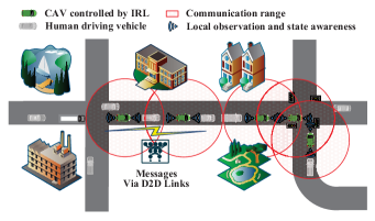
Figure 1: Illustration of MARL in autonomous driving.

TABLE I: The Summary of Differences with Related Literature.

References	Maximum Entropy	Policy Improvement Guarantee	Collaboration via Communication	Efficient Communication	Brief Description
[26-28]	$\CIRCLE$	$\Circle$	$\Circle$	$\Circle$	Only single-agent RL algorithm
[41-42]	$\Circle$	$\CIRCLE$	$\Circle$	$\Circle$
[33-35]	$\Circle$	$\Circle$	$\CIRCLE$	$\Circle$	Over frequent and complex communication
[40, 43]	$\Circle$	$\CIRCLE$	$\CIRCLE$	$\Circle$	Only under the traditional RL’s analysis
[18-23, 38-39]	$\Circle$	$\Circle$	$\CIRCLE$	$\CIRCLE$	Oversimplified parameter mixture method
Ours	$\CIRCLE$	$\CIRCLE$	$\CIRCLE$	$\CIRCLE$	Combining communication efficient DFL into MARL collaboration under maximum entropy framework with theory-established regulated mixture metrics
Notations: ${\Circle}$ indicates not included; ${\CIRCLE}$ indicates fully included.

I-B Related Works

Substantial research has been conducted in the field of IRL. For example, contingent on local observations, Independent $Q$-Learning (IQL) [11] allows agents to independently learn and update their own $Q$-value network. Independent Actor-Critic (IAC) [8] applies policy gradients by using an actor and a critic to approximate the policy and value function, respectively. Furthermore, Independent synchronous Advantage Actor-Critic (IA2C) [29] and Independent Proximal Policy Optimisation (IPPO) [30] adapt commonly-used A2C [31] and PPO [32] algorithms for decentralised multi-agent training. However, as IRL agents rely solely on their local perceptions without information sharing, this often results in varied policy performance and unstable learning.

As an extension of the classical IRL, distributed cooperative RL enhances agents’ collective capabilities and efficiency by collaboratively seeking near-optimal solutions through limited information exchange with others. Notably, the exchanged contexts can be rather different and possibly include approximated value functions in [33, 34], rewards or even maximal $Q$-values on each state-action pair in [35]. Besides, due to the privacy concern and communication restrictions (e.g., bandwidth or delay) in FRL, the direct exchange of model updates (i.e. gradients or parameters) during FL aggregation phase [14, 13, 36] is a viable way, given the clear evidence [37, 31] that experiences from homogeneous, independent learning agents in the same multi-agent system can contribute to efficiently learning a commonly shared Deep Neural Network (DNN) model. However, these works are typically based on a client-server architecture with an assumed existing central server, which might not always hold in practice.

On the other hand, the peer-to-peer DFL paradigm, wherein clients exchange their local models’ parameters or gradient information only with their neighbors to achieve model consensus, emerges as an appealing alternative. But the awful communication expenditure therein can not be ignored. In that regard, some researchers resort to reduce the communication frequency by merging more local updates before one round communication [18] or multi-round communication [19, 20]. Besides, either shrinking the number of parameters forwarded from local model or embarking on selective model synchronization is also tractable. Ref. [21] divides local gradients into several disjoint gradient partitions, with only a subset of these partitions being exchanged in any single communication round. Ref. [22] puts forward a randomized selection scheme for forwarding subsets of local model parameters to their one-hop neighbors. Ref. [23] introduces a segmented gossip approach that involves synchronizing only model segments, thereby substantially splitting the communication expenditure. Moreover, message size can be further reduced via gradient compression, quantization or sparsification [38, 20, 39].

Notably, when it comes to the method of mixing DNN parameters, these aforementioned DFL works generally adopt a simplistic averaging approach, which is familiar in parallel distributed Stochastic Gradient Descent (SGD) methods. However, when such an approach is directly applied into FRL, the crucial relationship between parameter gradient descent and policy improvement will be overshadowed [40]. Consequently, the corresponding mixture lacks proper, solid assessment means to prevent potential harm to policy performance [15]. In other words, directly using this kind of naive combination of communication efficient DFL and RL to enhance individual policy performance in IRL appears inefficient.

Regarding this issue, we can draw inspiration from the conservative policy iteration algorithm [41], which leverages the concept of policy advantage as a crucial indicator to gauge the improvement of the cumulative rewards, and applies a mixture update rule directly for policy distributions in its pursuit of an approximately optimal policy. Moreover, the mixture metric utilized in the update rule is also investigated to avoid making aggressive updates towards risky directions. This is particularly relevant as excessively large policy updates often lead to a significant deterioration of policy performance [15]. TRPO [42] substitutes the mixture metric with Kullback-Leibler (KL) divergence, a measure that quantifies the disparity between the distributions of the current and updated policies, and enables agents to learn monotonically improving policies. Ref. [43] extends this work into cooperative MARL settings. However, directly mixing policy distributions is often an intractable endeavor. To implement this procedure in practical settings with parameterised policies, Ref. [40] further simplifies the KL divergence to the parameter space through Fisher Information Matrix (FIM), so as to improve the policy performance by directly mixing DNN parameters. Nonetheless, these existing analyses are confined to the traditional RL, whose primary objective revolves around maximizing the expected return.

Transitioning to the realm of MERL, the integration of the entropy component marks a significant paradigm shift. This entropy term compels the adoption of policies that strive not only for reward maximization but also emphasize the importance of exploration. As a result, the criteria for policy improvement in MERL evolve to encompass dual objectives, that is, optimizing returns while simultaneously ensuring a consistent level of exploration throughout the learning process. This change necessitates a reevaluation of traditional RL methodologies, in which the previous conclusions may not adequately address the dynamic interplay between reward maximization and exploratory behavior imposed by the entropy maximization in MERL. On the other hand, it’s also imperative to implement an appropriate and manageable mixture metric with monotonic policy improvement property to maximize the practicality of directly mixing policy parameters during MARL communication phase. Such a metric must guarantee the efficacy of the resultant mixed policy in terms of policy improvement. Crucially, the assessment of the expected benefits of the mixed policy must be conducted before undertaking the actual policy mixing. That is, before any actual mixture of policy parameters, the potential of mixed policy to improve policy performance should be evaluated against the referential policy, whose parameters are received from neighbors in DFL. Only after confirming the anticipated benefits of the mixed policies should we proceed with the operation of mixing DNN parameters using the developed metric. Moreover, we have also summarized the key differences between our algorithm and the relevant literature in Table I. In conclusion, it is vital to reformulate the theoretical analysis within the combination of DFL and MERL framework, so as to offer robust theoretical underpinnings for practical applications in IoV.

I-C Contribution

TABLE II: Major notations used in the paper.

Notation	Definition
$s_{t}^{(i)},a_{t}^{(i)},r^{(i)}_{t}$	Local state, individual action and reward of agent $i$ at time step $t$
$\pi$, $\theta$	Current target policy and its parameters
$\tilde{\pi}$, $\tilde{\theta}$	The referential target policy and it parameters
$\pi_{\text{mix}},\theta_{\text{mix}}$	Mixed policy and its parameters
$p,P$	Index of segments, $p=1,2,\cdots,P$
$\Omega_{i}$	Set of one-hop neighbors within the communication range of agent $i$
$\zeta$	Mixture metric of current policy parameters and referential policy parameters
$\alpha$	Temperature parameter of policy entropy
$\varrho$	Target smoothing coefficient of target $Q$ networks
$\kappa$	Number of model replicas
$U$	Communication interval determined by specified iterations of the local policy
$\upsilon$	Size of the policy parameters
$\psi$	Communication consumption

In this paper, we propose the Regulated Segment Mixture-based Multi-Agent SAC (RSM-MASAC) algorithm, tailored for training local driving models of CAVs in the IoV using MERL while addressing communication overhead challenges inherent in DFL. Our primary contributions include:

• Innovative Combination of DFL and MERL: Different from the existing single-vehicle intelligence and centralized approaches, our framework innovatively combines DFL with MERL, adapted for IoV’s highly dynamic setting, eliminating the central controller and maintaining exploration to maximize learning performance.

• Communication Efficient MASAC Implementation: We present RSM-MASAC algorithm, designed to periodically and selectively receive segments of policy parameters from nearby vehicles within communication range to constitute referential policies for mixing, maximizing available bandwidth utilization and reducing communication overhead.

• Development of a Mixture Metric for Policy Improvement during Communication: We derive a manageable, theory-guided mixture metric with a monotonic policy improvement property, as well as regulate the selection of contributive referential policies, enhancing the practicality of directly mixing policy DNN parameters during MARL communication phase.

• Verified Performance through Extensive Simulations: Through extensive simulations in the traffic control scenarios, RSM-MASAC could approach the converged performance of centralized FMARL [13] in a distributed manner, outperforming parameter average methods as in DFL [23, 22], thus confirming its effectiveness.

I-D Paper Organization

The remainder of this paper is organized as follows. In Section II, we present preliminaries of SAC algorithm and main notations used in this paper. Then, we introduce the system model and formulate the problem in Section III. Afterwards, we elaborate on the details of the proposed RSM-MASAC algorithm in Section IV. In Section V, we present the simulation settings and discuss the experimental results. Finally, Section VI concludes this paper.

II Preliminary

Beforehand, we summarize the mainly used notations in Table II.

We consider the standard RL setting, where the learning process of each agent can be formulated as an MDP. During the interaction with the environment, at each time step $t$, an RL agent observes a local state $s_{t}$ from local state space $\mathcal{S}$, and chooses an action $a_{t}$ from individual action space $\mathcal{A}$ according to the policy $\pi(\cdot|s_{t})\in\Pi$, where $\Pi$ is the policy space. Then the agent receives an individual reward $r_{t}$, calculated by a reward function $\mathcal{R}:\mathcal{S}\times\mathcal{A}\rightarrow[0,R]$, and the environment transforms to a next state $s_{t+1}\sim p(\cdot|s_{t},a_{t})$. A trajectory starting from $s_{t}$ is denoted as $\tau_{t}=(s_{t},a_{t},s_{t+1},a_{t+1},\cdots)$. Besides, considering an infinite-horizon discounted MDP, the visitation probability of a certain state $s$ under the policy $\pi$ can be summarized as $d_{\pi}(s)=\sum\nolimits_{t=0}^{\infty}\gamma^{t}P(s_{t}=s;\pi)$, where $P(s_{t}=s;\pi)$ is the visitation probability of the state $s$ at time $t$ under the policy $\pi$.

Different from traditional RL algorithms aiming to maximize the discounted expected total rewards only, SAC [27, 28] additionally seeks to enhance the expected policy entropy. To be specific, with the re-defined soft state value function $V^{\pi}(s_{0}):=\mathop{\mathbb{E}}\limits_{\tau_{0}\sim\pi}\left[\sum_{t=0}^{\infty}\gamma^{t}(r_{t}+\alpha H(\pi(\cdot|s_{t})))\right]$ on top of the policy entropy $H(\pi(\cdot|s))=-\mathbb{E}_{a\sim\pi}\log\pi(a|s)$, the task objective of SAC can be formulated as

$$\vspace{-0.2em}\max\eta(\pi)=\mathop{\mathbb{E}}_{s_{0}\sim\rho_{0}}\left[V^{\pi}(s_{0})\right]$$ (1)

where $\rho_{0}$ is the distribution of initial state $s_{0}$ and $\alpha\in(0,\infty)$ is a temperature parameter determining the relative importance of the entropy term versus the reward. Obviously, when $\alpha\rightarrow 0$, SAC gradually approaches the traditional RL. Meanwhile, the soft state-action value can be expressed as $Q^{\pi}(s_{t},a_{t}):=r_{t}+\mathop{\mathbb{E}}_{\tau_{t+1}\sim\pi}\!\left[\sum_{l=t+1}^{\infty}\gamma^{l-t}\Big{(}r_{l}\!+\!\alpha H(\pi(\cdot|s_{l}))\Big{)}\!\right]$ [27, 28], which does not include the policy entropy of current time step but includes the sum of all future policy entropy and the sum of all current and future rewards. Consistently, the state-action advantage value under policy $\pi$ is

$$A_{\pi}(s_{t},a_{t})=Q^{\pi}(s_{t},a_{t})-V^{\pi}(s_{t})$$ (2)

Accordingly, SAC maximizes (1) based on soft policy iteration, which alternates between soft policy evaluation and soft policy improvement.

• For given $\pi$, soft policy evaluation implies that $Q^{\pi}$ is learned by repeatedly applying soft Bellman operator $\mathcal{T}^{\pi}$ to the real-valued estimate $Q$, given by:

  $$\mathcal{T}^{\pi}Q(s_{t},a_{t})=r_{t}+\gamma\mathbb{E}_{s_{t+1}\sim p(\cdot|s_{t},a_{t})}[V(s_{t+1})],$$ (3)

  where

  $$V(s_{t}) =\mathbb{E}_{a_{t}\sim\pi}[Q(s_{t},a_{t})]+\alpha H(\pi(\cdot|s_{t}))$$ (4)

  With $Q^{k+1}=\mathcal{T^{\pi}}Q^{k}$, as $k\rightarrow\infty$, $Q^{k}$ will converge to the soft $Q$ function $Q^{\pi}$ of $\pi$, as proven in [28].

• In the soft policy improvement step, the goal is to find a policy $\pi_{\text{new}}$ superior than the current policy $\pi_{\text{old}}$, in terms of maximizing (1). Specifically, for each state, SAC updates the policy as

  $$\pi_{\mathrm{new}}= \mathop{\arg\min}_{\pi\in\Pi}\mathrm{D}_{\mathrm{KL}}\Big{(}\pi(\cdot|s_{t})\|\frac{\exp\big{(}\frac{1}{\alpha}Q^{\pi_{\text{old}}}({s_{t}},\cdot)\big{)}}{Z^{\pi_{\text{old}}}(s_{t})}\Big{)}$$ (5)

  $$= \mathop{\arg\max}_{\pi\in\Pi}\mathbb{E}_{a_{t}\sim\pi}\left[Q^{\pi_{\text{old}}}(s_{t},a_{t})-\alpha\log\pi(a_{t}|s_{t})\right]$$

  where $\mathrm{D}_{\mathrm{KL}}(\cdot)$ denotes the KL divergence, while the partition function $Z^{\pi_{\text{old}}}$ normalizes the distribution. Since $Z^{\pi_{\text{old}}}$ has no contribution to gradient with respect to the new policy, it can thus be ignored. As unveiled in Appendix A, through the update rule of (5), $Q^{\pi_{\text{new}}}(s_{t},a_{t})\geq Q^{\pi_{\text{old}}}(s_{t},a_{t})$ is guaranteed for all $(s_{t},a_{t})\in\mathcal{S}\times\mathcal{A}$. Notably, the proof of soft policy improvement detailed in Appendix A additionally serves as a confirmation for policy improvement of regulated segment mixture, which will be elaborated upon later.

Finally, with repeated application of soft policy evaluation and soft policy improvement, any policy $\pi\in\Pi$ will converge to the optimal policy $\pi^{*}$ such that $Q^{\pi^{*}}(s_{t},a_{t})\geq Q^{\pi}(s_{t},a_{t}),\forall(s_{t},a_{t})\in\mathcal{S}\times\mathcal{A}$, and the proof can be found in [27, 28].

III System Model and Problem Formulation

III-A System Model

As illustrated in Fig. 1, we primarily consider an IoV scenario consisting of $N$ CAVs, in which each CAV is controlled by an independent SAC-empowered agent, alongside some human-driving vehicles. Our MASAC learning encompasses an independent local learning phase and a communication-assisted mixing phase. In the first phase, we use SAC algorithm for each IRL agent $i$, $i\in\{1,2,\cdots,N\}$. That is, agent $i$ senses partial status $s_{t}^{(i)}$ (e.g., the speed and positions of neighboring vehicles) of the IoV environment, and has its local policy $\pi^{(i)}$ parameterized by $\theta^{(i)}\in\mathbb{R}^{d}$. It collects samples $\langle s_{t}^{(i)},a_{t}^{(i)},r_{t}^{(i)},s_{t+1}^{(i)}\rangle$ in replay buffer $\mathcal{D}^{(i)}$, and randomly samples a mini-batch $\Phi^{(i)}$ for local independent model updates. Subsequently, in the second phase, each agent $i$ interacts with its one-hop neighbors $j\in\Omega_{i}$ within communication range, so as to reduce the behavioral localities of IRL and improve their cooperation efficiency. More specific, this communication can be done through standardized 3GPP sidelink communications (e.g., Device-to-Device [D2D] communications) without going through the network infrastructure [44].

III-A1 Local Learning Phase

Algorithmically, in the local learning phase with SAC, parameterized DNNs are used as approximators for policy and soft $Q$-function. Concretely, we alternate optimizing one policy network $\pi$ parameterized by $\theta$ and two soft $Q$ networks parameterized by $\omega_{1}$ and $\omega_{2}$, respectively. Besides, there are also two target soft $Q$ networks parameterized by $\bar{\omega}_{1}$ and $\bar{\omega}_{2}$, obtained as an exponentially moving average of current $Q$ network weights $\omega_{1}$, $\omega_{2}$. Yet, only the minimum $Q$ value of the two soft $Q$-functions is used for the SGD and policy gradient. This setting of two soft $Q$-functions will speed up training while the use of target $Q$ can stabilize the learning [27, 28, 45]. For training $\theta$ and $\omega\in{\omega_{1},\omega_{2}}$, agent randomly samples a batch of transition tuples from the replay buffer $\mathcal{D}$ and performs SGD. The parameters of each soft $Q$ network $\omega_{x},\forall x=1,2$ are updated through minimizing the soft Bellman residual error, that is,

$$\vspace{-0.2em}J_{Q}(\omega_{x})=\frac{1}{2}\mathop{\mathbb{E}}\nolimits_{s_{t},a_{t}\sim\mathcal{D}}\left[Q_{\omega_{x}}({s}_{t},{a}_{t})-\hat{Q}(s_{t},a_{t})\right]^{2}\vspace{-0.2em}$$ (6)

where the target $\hat{Q}(s_{t},a_{t})=r_{t}+\gamma\mathop{\mathbb{E}}_{\begin{subarray}{c}{s}_{t+1}\sim p(\cdot|s_{t},a_{t})\\ {a_{t+1}\sim\pi_{\theta}}\end{subarray}}\!\left[\mathop{\min}\limits_{x\in 1,2}Q_{\bar{\omega}_{x}}(s_{t+1},a_{t+1})\!-\!\alpha\log\pi_{\theta}(a_{t+1}|s_{t+1})\right]$.

Furthermore, the policy parameters of standard SAC can be learned according to (5) by replacing $Q^{\pi_{\text{old}}}$ with current $Q$ function estimate as

$$J_{\pi}(\theta)=\!\mathop{\mathbb{E}}\limits_{{s}_{t}\sim\mathcal{D}}\!\big{[}\!\mathop{\mathbb{E}}\limits_{{a}_{t}\sim\pi_{\theta}}\!\big{[}\alpha\log\pi_{\theta}({a}_{t}|{s}_{t})\!-\!\mathop{\min}_{\begin{subarray}{c}x\in 1,2\end{subarray}}Q_{\omega_{x}}({s}_{t},{a}_{t})\big{]}\big{]}\vspace{-0.2em}$$ (7)

Besides, since the gradient estimation of (7) has to depend on the actions stochastically sampled from $\pi_{\theta}$, which leads to high gradient variance, the reparameterization trick [27, 28] is used to decouple the action. Concretely, the random action $a_{t}$ can be expressed as a deterministic variable

$$\vspace{-0.2em}a_{t}=f_{\theta}(s_{t};\delta_{t})=\tanh\big{(}\mu_{\theta}(s_{t})+\delta_{t}\odot\sigma_{\theta}(s_{t})\big{)}\vspace{-0.2em}$$ (8)

where $\odot$ represents Hadamard product, and the action generation process is transformed into deterministic computation (i.e. the mean $\mu_{\theta}\in\mathbb{R}^{\dim\mathcal{A}}$ and standard deviation $\sigma_{\theta}\in\mathbb{R}^{\dim\mathcal{A}}$ of the output from policy network, parameterized by $\theta$) with added stochastic noise $\delta_{t}\sim\mathcal{N}(0,\mathbf{I}_{\dim\mathcal{A}})$, allowing for a balance between exploration and stable, efficient gradient-based training.

In addition to the soft $Q$-function and the policy, the temperature parameter $\alpha$ can be automatically updated by optimizing the following loss

$$J(\alpha)=\mathop{\mathbb{E}}\limits_{s_{t}\sim\mathcal{D}}\big{[}\mathop{\mathbb{E}}_{{a}_{t}\sim\pi_{\theta}}[-\alpha\log\pi_{\theta}({a}_{t}|{s}_{t})-\alpha\bar{\mathcal{H}}]\big{]}\vspace{-0.2em}$$ (9)

where $\bar{\mathcal{H}}$ is an entropy target with default value $-\dim{\mathcal{A}}$. Thus the policy can explore more in regions where the optimal action is uncertain, and remain more deterministic in states with a clear distinction between good and bad actions.

In addition, since two-timescale updates, i.e, less frequent policy updates, usually result in higher quality policy updates. Therefore, we integrate the delayed policy update mechanism employed in TD3 [46], into our framework’s methodology. To this end, the policy, temperature and target $Q$ networks are updated with respect to soft $Q$ network every $d$ iterations.

III-A2 Communication-Assisted Mixing Phase

Subsequent to the phase of local learning, neighboring agents initiate periodic communication to enhance their collaboration in accomplishing complex tasks. Considering the possible communication bandwidth or delay restriction between agents in real-world facilities, we assume messages transmitted by agents are limited to policy parameters $\theta$. Such an assumption is also feasible, as soft $Q$-functions have less impact on the action selection than the policy in actor-critic algorithm.

Specifically, every $U$ times of policy updates, a communication round begins. Agent $i$ acquires the policy parameters $\theta^{(j)}$ from neighboring agents $j\in\Omega_{i}$ via the D2D collaboration channel. Subsequently, agent $i$ could employ various methods to formulate a referential policy $\tilde{\pi}^{(i)}$, which is parameterized by $\tilde{\theta}^{(i)}\!=\!f({\theta}^{(1)},\cdots,{\theta}^{(j)},\cdots)$, leveraging the parameters obtained from its neighbors $\forall j\in\Omega_{i}$.

Afterwards, agent $i$ directly mixes DNN parameters of the policy network, consistently with parallel distributed SGD methods as

$$\theta_{\text{mix}}^{(i)}=\theta^{(i)}+\zeta(\tilde{\theta}^{(i)}-\theta^{(i)})\vspace{-0.1em}$$ (10)

where $\zeta\in[0,1]$ is the mixture metric of DNN parameters. Taking model averaging in [19, 40] as example, $\tilde{\theta}^{(i)}$ is computed as $\tilde{\theta}^{(i)}\!=\!\sum\nolimits_{j\in\Omega_{i}}\!{\theta}^{(j)}$, and $\zeta\!=\!1\!-\!1/|\Omega_{i}|$ further influenced by the number of neighbors involved. Then, for each agent $i$, $\theta^{(i)}$ should get aligned with mixed policy’s parameters $\theta_{\text{mix}}^{(i)}$.

III-B Problem Formulation

This paper primarily targets the communication assisted mixing phase in MASAC. Intuitively, an effective mixture means could better leverage the exchanged parameters to yield a superior target referential policy, which has a higher value with respect to the maximum entropy objective as in (1). However, it remains little investigated on the feasible means to mix the exchanged parameters (or their partial segments) and determine the proper mixture metric in (10), though it vitally affects both the communication overhead and learning performance. Therefore, by optimizing both $f$ and $\zeta$, we mainly focus on reducing the communication expenditure while maintain acceptable cumulative rewards, that is,

$$\min_{f,\zeta}c(\upsilon,f)$$

$$s.t.\quad \sum\nolimits_{t}r_{t}(\Theta,\zeta)\geq r^{\text{thre}}$$

$$\Theta\leftarrow\{\theta_{\text{mix},k}^{(1)},\cdots,\theta_{\text{mix},k}^{(N)}\}$$ (11)

$$\theta_{\text{mix},k}^{(i)}=\theta_{k}^{(i)}+\zeta(\tilde{\theta}_{k}^{(i)}-\theta_{k}^{(i)}), \forall i\in\{1,\cdots,N\}$$

$$\tilde{\theta}_{k}^{(i)}=f({\theta}_{k}^{(1)},\cdots,{\theta}_{k}^{(j)},\cdots), \forall k\text{ mod }U=0,j\in\Omega_{i}$$

where $r^{\text{thre}}$ denotes the required minimum cumulative rewards, $v$ indicates the size of policy parameters, and $k$ is the index of policy iterations. Furthermore, $c(v,f)$ denotes the communication expenditure, which is governed by the mixture function $f$. For example, for the whole policy parameter transmission among all agents [40], the total communication cost per round is $c(\upsilon,f)\!=\!N\!\times\!(N-1)\!\times\!\upsilon$. Apparently, the communication cost $c(\upsilon,f)$ can be significantly reduced, if $f$ could rely on fewer agents with reduced communication frequency. However, such a naive design possibly mitigates the positive effect of collaboration as well. Therefore, it is worthwhile to resort to a more comprehensive design of $f$ and $\zeta$ to calibrate the communicating agents and content as well as regulate the mixture means, so as to provide a guarantee of performance improvement.

IV MASAC with Regulated Segment Mixture

In this section, as shown in Fig. LABEL:fig:framework, we present the design of RSM-MASAC, which reduces the communication overhead while incurring little sacrifice to the learning performance.

IV-A Algorithm Design

Consistent with the SAC setting as in Section III, agents in RSM-MASAC undergo the same local iteration process. Meanwhile, for the communication-assisted mixing phase, we will elaborate on the design details of RSM-MASAC, including the segment request & response, criterion for reconstructed referential policy selection, and policy parameter mixture with theory-established performance improvement.

IV-A1 Segment Request & Response

Inspired by segmented pulling synchronization mechanism in DFL [47], we develop and perform a segment request & response procedure. This approach allows each agent to selectively request various segments of policy parameters from different neighbors, thereby facilitating the construction of a reconstructed referential policy for subsequent aggregation while also balancing the load of communication costs. Specifically, for every communication round, agent $i$ breaks its policy parameters $\theta^{(i)}$ into $P$ ($P\leq|\Omega_{i}|$) non-overlapping segments $\hat{\theta}^{(i)}_{1},\hat{\theta}^{(i)}_{2},\cdots,\hat{\theta}^{(i)}_{P}$ as

$$\theta^{(i)}=(\hat{\theta}^{(i)}_{1},\hat{\theta}^{(i)}_{2},\cdots,\hat{\theta}^{(i)}_{P})\vspace{-0.1em}$$ (12)

Significantly, the available segmentation strategies are diverse and include, but not limited to, dividing the policy parameters by DNN layers, distributing based on the quantity of samples amassed by each agent, or segmenting according to the overall parameter size, etc.

Here, we use the most intuitive uniform parameter partition to clarify this process. For each segment $p=1,\cdots,P$, agent $i$ randomly selects a target agent (without replacement) from its neighbors (i.e., $j_{p}\in\Omega_{i}$) to send segment request $(i,P,j_{p},p)$, which indicates the agent $i$ who initiates the request and its total segment number $P$, as well as the requested segment $p$ from the target agent $j_{p}$. Upon receiving the request, the agent $j_{p}$ will break its own policy parameters $\theta^{(j_{p})}$ into $P$ segments and return the corresponding requested segment $\hat{\theta}^{(j_{p})}_{p}$ according to the identifier $p$. The number of segments $P$ can be flexibly determined according to the actual communication range of the agent. It should be noted that in order to reduce the complexity and facilitate the implementation, we only discuss the case as in Fig. LABEL:fig:framework that $P$ is the same constant for all agents and is not greater than $\max_{i}|\Omega_{i}|,\forall i$. Meanwhile, the segmentation methodology is identical across agents. Then, agent $i$ could reconstruct a referential policy based on all of the fetched segments, that is,

$$\tilde{\theta}^{(i)}=(\hat{\theta}^{(j_{1})}_{1},\hat{\theta}_{2}^{(j_{2})},\cdots,\hat{\theta}_{P}^{(j_{P})})\vspace{-0.1cm}$$ (13)

In fact, this segmented transmission approach can be executed in parallel, thereby optimizing the utilization of available bandwidth. Instead of being confined to a single link, the traffic is distributed across $P$ links, enhancing the overall data transfer efficiency. Besides, in order to further accelerate the propagation and ensure the model quality, we can construct multiple model replicas in RSM-MASAC. That is, the process of segment request $\&$ response can be repeated $P\times\kappa$ times, reconstructing $\kappa$ reconstructed referential policies in one communication round.

IV-A2 Criterion for Reconstructed Referential Policy Selection

Algorithm 1 RSM-MASAC Algorithm

1:  Initialize network parameters $\theta^{(i)}$, $\omega_{1}^{(i)}$, $\omega_{2}^{(i)}$, $i=1,2,\cdots N$

2:  Initialize target network parameters $\bar{\omega}_{1}^{(i)}\leftarrow\omega_{1}^{(i)}$, $\bar{\omega}_{2}^{(i)}\leftarrow\omega_{2}^{(i)}$

3:  Initialize learning rate $\eta_{\pi}$, $\eta_{Q}$, $\eta_{\alpha}$, temperature $\alpha$, communication interval $U$, number of segments $P$ and number of replicas $\kappa$

4:  Initialize iteration index $k\leftarrow 0$ and $counter\leftarrow 0$

5:  for each epoch do

6:     for $t\leftarrow 1$ to $T$ do

7:        Each agent $i$ executes:

8:        * Independent local learning phase

9:        Select an action $a_{t}^{(i)}$ with respect to $s_{t}^{(i)}$ according to the current policy $\pi^{(i)}$ parameterized by $\theta^{(i)}$

10:        Observe reward $r_{t}^{(i)}$ and next state $s_{t+1}^{(i)}$

11:        Save the new transition in replay buffer: $\mathcal{D}^{(i)}\leftarrow\mathcal{D}^{(i)}\cup\langle s_{t}^{(i)},a_{t}^{(i)},r_{t}^{(i)},s_{t+1}^{(i)}\rangle$

12:        Sample a mini-batch $\Phi^{(i)}\sim\mathcal{D}^{(i)}$

13:        Update soft $Q$ function $\omega_{x}^{(i)}\leftarrow\omega_{x}^{(i)}-\eta_{Q}\nabla J_{Q}(\omega_{x}^{(i)})$ by (6), for $\forall x={1,2}$

14:        if $counter\bmod d=0$ or $t=T$ then

15:           Update policy $\vspace{-0.5em}\theta_{k+1}^{(i)}\leftarrow\theta_{k}^{(i)}-\eta_{\pi}\nabla J_{\pi}(\theta_{k}^{(i)})$ by (7)

16:           Adjust temperature $\alpha^{(i)}\leftarrow\alpha^{(i)}-\eta_{\alpha}\nabla J(\alpha^{(i)})$ by (9)

17:           Update target networks $\bar{\omega}_{x}^{(i)}\leftarrow\varrho\omega_{x}^{(i)}+(1-\varrho)\bar{\omega}_{x}^{(i)}$, for $\forall x=1,2$

18:           $k\leftarrow k+1$

19:        end if

20:        $counter\leftarrow counter+1$

21:        * Communication-assisted mixing phase

22:        if $k\bmod U=0$ then

23:           Update policy $\theta_{k}^{(i)}\leftarrow$ CommMix($\theta_{k}^{(i)}$, $i$, $\Omega_{i}$, $P$, $\kappa$)

24:        end if

25:     end for

26:  end for   

27:  CommMix($\theta,i,\Omega_{i},P,\kappa$):

28:       for each replica $u=1,2,\cdots,\kappa$ do

29:           Send $P$ pulling request $(i,P,j_{p},p)$ to nearby collaborators   in $\Omega_{i}$, and receive $\hat{\theta}^{(j_{p})}_{p}$ to reconstruct $\tilde{\theta}$ as (13)

30:           Select $M$ samples from the replay buffer $\mathcal{D}^{(i)}$

31:           Estimate $\mathbb{A}^{+}_{\pi}(\tilde{\pi})$ according to (19)

32:           if $\mathbb{A}^{+}_{\pi}(\tilde{\pi})>0$ then

33:               Evaluate $F(\theta)$ according to (20)

34:               Get the upper bound of $\zeta$ according to Theorem 2

35:               Make the mixture metric $\zeta$ less than the calculated upper    bound, and update $\theta_{\text{mix}}^{(i)}$ by (10)

36:              $\quad\theta\leftarrow\theta_{\text{mix}}^{(i)}$

37:           end if

38:       end for

Given the potential for significant variability in policy performance due to differences in the training samples among multiple agents, it is critical to recognize that not all reconstructed referential policies - those amalgamated with the agent’s own policy via the DNN parameter mixture approach detailed in (10) - can contribute to agent’s local learning process. More seriously, it may even degrade the learning performance sometimes. Therefore, in order to ensure the policy improvement post-mixture, a robust theoretical analysis method for evaluating the efficacy of the mixed policy $\pi_{\text{mix}}$, parameterized by $\theta_{\text{mix}}$, is essential. This would regulate the selection of only those referential policies $\tilde{\pi}$, parameterized by $\tilde{\theta}$, that are beneficial, into the parameter mixture process.

Drawing from this premise, based upon the conservative policy iteration as outlined in [41], we employ a mixture update rule on policy distributions to find an approximately optimal policy. Our analysis here will also focus specifically on the mixing of policy distributions that exhibit a monotonic policy improvement property during the communication phase. The detailed and more practical implementation of the policy DNN parameters’ mixture rule derived from this section will be thoroughly presented in the next subsection.

For any state $s$, we also define the mixed policy $\pi_{\text{mix}}$, which refers to a mixed distribution, as the linear combination of any reconstructed referential policy $\tilde{\pi}$ and current policy $\pi$

$$\pi_{\text{mix}}(a|s)=(1-\beta)\pi(a|s)+\beta\tilde{\pi}(a|s)$$ (14)

where $\beta\in[0,1]$ is the weighting factor. The soft policy improvement, as outlined in Appendix A, suggests that this policy mixture can influence the ultimate performance regarding the objective stated in (1). Fortunately, we have the following new theorem on the performance gap associated with adopting these two different policies.

Theorem 1.

(Mixed Policy Improvement Bound) For any policy $\pi$ and $\tilde{\pi}$ adhering to (14), the improvement in policy performance after mixing can be measured by:

$$\eta(\pi_{\text{mix}})-\eta(\pi) \geq\beta\mathop{\mathbb{E}}_{\begin{subarray}{c}s\sim d_{\pi}\\ a\sim\tilde{\pi}\end{subarray}}\left[A_{\pi}(s,a)+\alpha H(\tilde{\pi}(\cdot|s))\right]-\frac{2\gamma\varepsilon\beta^{2}}{(1-\gamma)^{2}}$$

$$\quad+\alpha\mathop{\mathbb{E}}_{s\sim d_{\pi_{\text{mix}}}}\left[\mathrm{D}_{\mathrm{JS}}^{\beta}(\tilde{\pi}(\cdot|s)\|\pi(\cdot|s))\right]$$ (15)

where $\varepsilon\!:=\!\max_{s}|\mathop{\mathbb{E}}_{a\sim\tilde{\pi}}[A_{\pi}(s,a)\!+\!\alpha H(\tilde{\pi}(\cdot|s))]|$ represents the maximum advantage of $\tilde{\pi}$ relative to $\pi$, and $\mathrm{D}_{\mathrm{JS}}^{\beta}(p\|q)=\beta\sum p\log\frac{p}{\beta p+(1-\beta)q}+(1-\beta)\sum q\log\frac{q}{\beta p+(1-\beta)q}$ is the $\beta$-skew Jensen-Shannon(JS)-symmetrization of KL divergence [48], with two distributions $p$ and $q$.

The proof of this theorem is given in the Appendix B.

Remark: The mixed policy improvement bound in (1) implies that under the condition that the right-hand side of (1) is larger than zero, the mixed policy will assuredly lead to an improvement in the true expected objective $\eta$. Besides, from another point of view, any mixed policy with a guaranteed policy improvement in Theorem 1 definitely satisfies the soft policy improvement as well, since the item $\mathbb{E}_{s_{1}}\left(\alpha H(\pi_{\text{old}}(\cdot|s_{1}))\!+\!\mathop{\mathbb{E}}_{\begin{subarray}{c}a_{1}\sim\pi_{\text{old}}\end{subarray}}[Q^{\pi_{\text{old}}}(s_{1},a_{1})]\right)=\mathbb{E}_{s_{1}}[V^{\pi_{\text{old}}}(s_{1})]$ in (21) in the Appendix A (i.e., proof of Lemma 1) is less than $\mathbb{E}_{s_{1}}[V^{\pi_{\text{mix}}}(s_{1})]$. In addition, when the temperature parameter $\alpha=0$, this inequality can reduce to the standard form of policy improvement in traditional RL [41, 42, 40]. Hence, Theorem 1 derives a more general conclusion for both MERL and traditional RL.

Furthermore, since for $\beta\in[0,1]$, $D_{\text{JS}}^{\beta}$ is greater than zero [48]. Therefore, we only need to consider the sign of the first two terms in (1). By definition of a policy advantage

$$\mathbb{A}^{+}_{\pi}(\tilde{\pi}):=\mathop{\mathbb{E}}_{\begin{subarray}{c}s\sim d_{\pi},a\sim\tilde{\pi}\end{subarray}}\left[A_{\pi}(s,a)+\alpha H(\tilde{\pi}(\cdot|s))\right]$$ (16)

we can therefore establish a tighter yet more tractable bound for policy improvement as

$$\eta(\pi_{\text{mix}})-\eta(\pi) \geq\beta\mathbb{A}^{+}_{\pi}(\tilde{\pi})-C\beta^{2}$$ (17)

where $C=\frac{2\varepsilon\gamma}{(1-\gamma)^{2}}$. Thus, (17) indicates that a mixed policy conforms to the principle of soft policy improvement, provided that the right-side of (17) yields a positive value. More specific, if the policy advantage $\mathbb{A}^{+}_{\pi}(\tilde{\pi})$ is positive, an agent with policy $\pi$ can reap benefits by mixing its policy distribution with reconstructed referential policy $\tilde{\pi}$. On the contrary, if this advantage is non-positive, policy improvement cannot be assured through the mixing of $\tilde{\pi}$ and $\pi$. In essence, (17) serves as a criterion for selecting referential policies that ensure final performance improvement, and thus we have the following corollary.

Corollary 1.

In order to obtain guaranteed performance improvement, the mixture approach of policy distributions shall satisfy that

• $\mathbb{A}^{+}_{\pi}(\tilde{\pi})>0$;

• $\beta\mathbb{A}^{+}_{\pi}(\tilde{\pi})-C\beta^{2}>0$.

The detailed and more practical mixture process will be described in the next subsection.

IV-A3 Policy Parameter Mixture with Theory-Established Performance Improvement

Consistent with TRPO [42], we introduce KL divergence to replace $\beta$ by setting $\beta:=\sqrt{\mathrm{D}_{\mathrm{KL}}^{\max}(\pi\|\pi_{\text{mix}})}$, where $\mathrm{D}_{\mathrm{KL}}^{\max}(\pi\|\pi_{\text{mix}})=\max_{s}\mathrm{D}_{\mathrm{KL}}(\pi(\cdot|s)\|\pi_{\text{mix}}(\cdot|s))$. Thus, the second condition in Corollary 1 is equivalent to

$$\vspace{-0.2em}\sqrt{\mathrm{D}_{\mathrm{KL}}^{\max}(\pi\|\pi_{\text{mix}})}<\frac{\mathbb{A}^{+}_{\pi}(\tilde{\pi})}{C}.\vspace{-0.2em}$$ (18)

Nevertheless, it hinges on the computation-costly KL divergence to quantify the difference between probability distributions. Fortunately, since for a small change in the policy parameters, the KL divergence between the original policy and the updated policy can be approximated using a second-order Taylor expansion, wherein FIM serves as the coefficient matrix for the quadratic term. This provides a tractable way to assess the impact of parameter changes on the policy. Therefore, we utilize FIM, delineated in context of natural policy gradients by [49], as a mapping mechanism to revise the impact of certain changes in policy parameter space on probability distribution space. Then in the following theorem, we can get the easier-to-follow, trustable upper bound for the mixture metric of policy DNN parameters.

Theorem 2.

(Guaranteed Policy Improvement via Parameter Mixing Conditions) With any reconstructed referential policy parameters $\tilde{\theta}$, an agent with current policy parameters $\theta$ can improve the true objective $\eta$ as in (1) through updating $\theta$ to mixed policy parameters $\theta_{\text{mix}}$ in accordance with (10), provided it fulfills the following two conditions:

• $\mathbb{A}^{+}_{\pi}(\tilde{\pi})>0$;

• $0<\zeta<\left[\frac{2\mathbb{A}^{+}_{\pi}(\tilde{\pi})}{C[(\tilde{\theta}-\theta)^{\intercal}F(\theta)(\tilde{\theta}-\theta)]}\right]^{\frac{1}{2}}$.

where $F(\theta)$ is the FIM of policy $\pi$ parameterized by $\theta$.

Proof.

Recalling the definition of $\beta$ and the mixture approach of $\theta_{\text{mix}}$ in (10), as well the change of policy parameters (i.e., $\Delta\theta=\zeta(\tilde{\theta}-\theta)$), for any state $s$, the KL divergence between the current policy and the mixed policy can be expressed by performing a second-order Taylor expansion of the KL divergence at the point $\theta$ in parameter space as

$$\vspace{-3em}\mathrm{D}_{\mathrm{KL}} (\pi_{\theta}(\cdot|s)\|\pi_{\theta+\Delta\theta}(\cdot|s))$$

$$= \sum_{a\in\mathcal{A}}\pi_{\theta}(a|s)\log\frac{\pi_{\theta}(a|s)}{\pi_{\theta+\Delta\theta}(a|s)}$$

$$\approx \mathrm{D}_{\mathrm{KL}}(\pi_{\theta}(\cdot|s)\|\pi_{\theta}(\cdot|s))-\mathop{\mathbb{E}}\limits_{a\sim\pi_{\theta}}\left[\frac{\partial\log\pi_{\theta}(a|s)}{\partial\theta}\right]^{\intercal}\!\!\Delta\theta$$

$$\quad+\frac{1}{2}\Delta\theta^{\intercal}F(\theta)\Delta\theta$$

$$\stackrel{{\scriptstyle(a)}}{{=}} \frac{1}{2}\zeta^{2}(\tilde{\theta}-\theta)^{\intercal}F(\theta)(\tilde{\theta}-\theta)\vspace{-2em}$$

where the equality $(a)$ comes from the fact that by definition, $\mathrm{D}_{\mathrm{KL}}(\pi_{\theta}(\cdot|s)\|\pi_{\theta}(\cdot|s))=0$, while $\mathop{\mathbb{E}}\nolimits_{a\sim\pi_{\theta}}\left[\frac{\partial\log\pi_{\theta}(a|s)}{\partial\theta}\right]=\sum_{a\in\mathcal{A}}\pi_{\theta}(a|s)\frac{\partial\log\pi_{\theta}(a|s)}{\partial\theta}=\sum_{a\in\mathcal{A}}\frac{\partial\pi_{\theta}(a|s)}{\partial\theta}=0$. Notably, the FIM $F(\theta)$ takes the expectation for all possible states, which reflects the average sensitivity of the whole state space rather than a particular state, and can be calculated as

$$\vspace{-0.5em}F(\theta)=\mathop{\mathbb{E}}_{\begin{subarray}{c}s\sim d_{\pi}\\ a\sim\pi_{\theta}\end{subarray}}\left[\left(\frac{\partial\log\pi_{\theta}(a|s)}{\partial\theta}\right)\!\left(\frac{\partial\log\pi_{\theta}(a|s)}{\partial\theta}\right)^{\intercal}\right]$$

Finally, combining Corollary 1 and (18), we have the theorem. ∎

Remark: With Theorem 1 and Theorem 2, we can anticipate the extent of policy performance changes resulting from policy DNN parameters mixture during communication phase. This prediction is based solely on the local curvature of the policy space provided by FIM, thus avoiding the cumbersome computations to derive the full KL divergence of two distributions for every state. Besides, given that $F(\theta)$ is a positive definite matrix, a positive sign of the policy advantage $\mathbb{A}^{+}_{\pi}(\tilde{\pi})$ implies an increase in the DNN parameters’ mixture metric $\zeta$ corresponding to the rise in $\mathbb{A}^{+}_{\pi}(\tilde{\pi})$. That is, rather than simple averaging, agents can achieve guaranteed soft policy improvement after mixing by learning more effectively from reconstructed referential policies with an elevated $\zeta$.

In practice, to evaluate $\mathbb{A}^{+}_{\pi}(\tilde{\pi})$ and $F(\theta)$, the expectation can be estimated by the Monte Carlo method, approximating the global average by the states and actions under the policy. Meanwhile, the importance sampling estimator is also adopted to use the off-policy data in replay buffer for the policy advantage estimation, where $\pi_{t}$ typically denotes the action sampling policy at time step $t$. As outlined in Lemma 7 in Appendix C, we have

$$\mathbb{A}^{+}_{\pi}(\tilde{\pi}) \approx\mathbb{E}_{s_{t},a_{t}\sim\mathcal{D}}\bigg{[}\left(\frac{\tilde{\pi}_{\tilde{\theta}}(a_{t}|s_{t})-\pi_{\theta}(a_{t}|s_{t})}{\pi_{t}(a_{t}|s_{t})}\right)\!\mathop{\min}_{\begin{subarray}{c}x\in 1,2\end{subarray}}Q_{\omega_{x}}({s}_{t},{a}_{t})$$

$$\qquad+\alpha[H(\tilde{\pi}_{\tilde{\theta}}(\cdot|s_{t}))-H({\pi}_{{\theta}}(\cdot|s_{t}))]\bigg{]}$$ (19)

and

$$F(\theta)\!\approx\!\mathop{\mathbb{E}}\limits_{s_{t}\sim\mathcal{D}}\!\bigg{[}\!\mathop{\mathbb{E}}\limits_{a_{t}\sim\pi_{\theta}}\!\bigg{[}\!\left(\frac{\partial\log\pi_{\theta}(a|s)}{\partial\theta}\right)\!\left(\frac{\partial\log\pi_{\theta}(a|s)}{\partial\theta}\right)^{\intercal}\!\bigg{]}\bigg{]}$$ (20)

We opt for a sampling-based method for simplicity in our approach, yet the actual computation of the FIM is not restricted to this method alone. Considering models with a large number of parameters, there is extensive research on FIM approximation methods, such as Diagonal Approximation [50, 51], Low-Rank Approximation [52], etc.

Finally, we summarize the details of RSM-MASAC in Algorithm 1. RSM-MASAC employs a theory-guided metric for policy parameter mixture, which takes into account the potential influence of parameters mixture on soft policy improvement under MERL — a factor commonly overlooked in parallel distributed SGD methodologies. In particular, the mixing process between any two agents is initiated solely when there is a positive policy advantage. Adhering to Theorem 2, the mixture metric is set marginally below its computed upper limit, ensuring both the policy improvement and the convergence.

IV-B Communication Cost Analysis

In this subsection, we will analyse the communication efficiency of RSM-MASAC. Notably, since the pulling request does not contain any actual data, its cost in the analysis can be ignored, and we only consider the policy parameters transmitted among agents.

Regarding the communication overhead for each segment request, RSM-MASAC incurs a data transmission cost of $\upsilon_{p}=\upsilon/P$ through D2D communications. Consequently, the total communication overhead for reconstructing $\kappa$ referential policies per agent in each round $c(\upsilon,f)=N\times\upsilon\times\kappa$, which is $(N-1)/\kappa$ times less than that in a fully connected communication setup [40]. Additionally, communication occurs at a periodic interval of $U$, allowing for further reduction in communication overhead by decreasing communication frequency. Moreover, by simultaneously requesting $P$ agents in parallel, RSM-MASAC benefits the sufficient use of the bandwidth and enhances the capability to overcome possible channel degradation.

V Experimental Results and Discussions

In this section, we validate the effectiveness of our proposed algorithm for CAVs control in IoV, highlighting its superiority compared to other methods.

V-A Experimental Settings

We implement two simulation scenarios on Flow [53, 54], which is a traffic control benchmarking framework for mixed autonomy traffic. As inllustrated in Fig. LABEL:fig:benchmark, the scenarios of “Figure 8” and “Merge” are selected, with the main system settings described in Table III.

TABLE III: Setting of System Parameters in two scenarios.

Parameters Definition	Figure Eight	Merge
Number of DRL agents $N$	$9$	$13$
Total time-steps per epoch $T$	$1,500$	$750$
Number of epochs	$300$	$300$
Range of acceleration ($m/s^{2}$)	$[-3,3]$	$[-1.5,1.5]$
Desired velocity per vehicle ($m/s$)	$20$	$20$
Speed limit per vehicle ($m/s$)	$30$	$30$
Length per time-step (s)	$0.1$	$0.1$
Maximum of vehicles per hour	-	$2,300$

• In the first scenario “Figure 8”, $14$ vehicles navigate a one-way lane shapes like a figure “8”, including $5$ emulated human-driven vehicles controlled by Simulation of Urban MObility (SUMO) with Intelligent Driver Model (IDM) [55], and $9$ IRL-controlled CAVs maintaining dedicated links to update their parameters through the D2D channel. At the lane’s intersection, each CAV adjusts its acceleration to traverse efficiently, aiming to boost the traffic flow’s average speed.

• The second “Merge” scenario simulates highway on-ramp merging, and it’s also essential for CAVs to manage collision avoidance and congestion at merge points. The simulation settings closely align with those of the first scenario. Moreover, “Merge” caps vehicle flow at $2,300$ per hour, including a maximum of $2,200$ vehicles on the main road and $100$ vehicles on the ramp. Within each epoch, $13$ vehicles are randomly chosen to instantiate the DRL-based controllers.

Both two scenarios are modified to assign the limited partial-observation of global environment as the state of each vehicle, including the position and speed of its own, the vehicle ahead and behind. Meanwhile, each CAV’s action is a continuous variable representing the speed acceleration or deceleration and is normalized between $[-1,1]$. In order to reduce the occurrence of collisions and promote the traffic flow to the maximum desired speed, we take the normalized average speed of all vehicles at each timestep as the individual reward in each scenario, which is assigned to each training vehicle after its action being performed. In addition, the current epoch will be terminated once a collision occurs or the max length of step $T$ in an epoch is reached.

We perform tests every $10$ epochs and calculate the average reward based on the accumulated rewards from $5$ independent testing epochs. Besides, all results are produced by taking the average of $5$ independent simulations. Moreover, as for the baseline, we take the vehicles controlled by the Flow IDM [55], which belongs to a typical car-following model incorporating extensive prior knowledge and indicates the pinnacle of performance achievable by the best centralized federated MARL algorithms [13]. Furthermore, the principal hyper-parameters used in simulations are listed in Table IV.

TABLE IV: Hyper-parameters.

Hyper-parameters	Symbol	Value
Replay buffer size	$|\mathcal{D}|$	$10^{5}$
Batch size	$\Phi$	$256$
Number of samples to evaluate $\mathbb{A}^{+}_{\pi}(\tilde{\pi})$ and $F(\theta)$	$M$	$256$
Learning rate of actor network	$\eta_{\pi}$	$10^{-4}$
Learning rate of critic network	$\eta_{Q}$	$3\times 10^{-3}$
Learning rate of temperature parameter	$\eta_{\alpha}$	$3\times 10^{-4}$
Discount factor	$\gamma$	$0.99$
Target smoothing coefficient	$\varrho$	$10^{-3}$
Delayed policy update intervals	$d$	$10$
Communication intervals	$U$	$8$
Number of segments	$P$	4
Number of model replicas	$\kappa$	3

V-B Evaluation Metrics

Apart from the average reward, we adopt some additional metrics to extensively evaluate communication efficiency of RSM-MASAC.

• We denote the total count of reconstructed referential policies (i.e., all model replicas) as $\rho_{\text{total}}$. And the number of effectively reconstructed referential policies, those contributing to the mixing process, is represented by $\rho_{\text{ef}}$. The mixing rate $\rho_{r}=\rho_{\text{ef}}/\rho_{\text{total}}$ thus reflects the usage rate of reconstructed policies.

• We use $\psi$ to indicate the overall communication overhead (in terms of $\upsilon$) in an epoch, and $C_{0}$ denotes the number of communication rounds. Therefore, the communication overheads equal $\psi=C_{0}\times c(\upsilon,f)=\rho_{\text{total}}\times\upsilon$.

Intuitively, the average reward and communication efficiency will be determined by the function design of $f$, as well as the number of model segments and model replicas (i.e., $P$ and $\kappa$). Besides, the communication overhead is also affected by communication intervals $U$.

V-C Simulation Results

TABLE V: Results of Average Reward & Communication Efficiency under “Merge” scenario.

Method		$U$	$P$	$\kappa$	Average Reward	$\rho_{\text{total}}$	$\psi$	$\rho_{\text{ef}}$	$\rho_{r}$
Avg-	MAPPO	$8$	$4$	$3$	$0.5940\pm 0.0204$	$24,381$	$24,381\times\upsilon$	$24,381$	$100\%$
	MASAC				$0.6584\pm 0.0107$	$43,797$	$43,797\times\upsilon$	$43,797$	$100\%$
RSM-	MAPPO				$0.6173\pm 0.0097$	$24,381$	$24,381\times\upsilon$	$10,294$	$42.22\%$
	MASAC			$1$	$0.6648\pm 0.0065$	$14,599$	$14,599\times\upsilon$	$7,938$	$54.37\%$
				$5$	$0.6745\pm 0.0120$	$72,995$	$72,995\times\upsilon$	$33,484$	$45.87\%$
				$7$	$0.6721\pm 0.0072$	$102,102$	$102,102\times\upsilon$	$47,122$	$46.15\%$
				$3$	$0.6658\pm 0.0063$	$43,797$	$43,797\times\upsilon$	$22,661$	$51.74\%$
			$1$		$0.6654\pm 0.0048$	$43,797$	$43,797\times\upsilon$	$21,024$	$48.00\%$
			$2$		$0.6677\pm 0.0064$	$43,797$	$43,797\times\upsilon$	$21,083$	$48.14\%$
			$6$		$0.6656\pm 0.0059$	$43,797$	$43,797\times\upsilon$	$22,128$	$50.52\%$
		$72$	$4$		$0.6464\pm 0.0292$	$4,875$	$4,875\times\upsilon$	$2,345$	$48.10\%$
		$144$			$0.6455\pm 0.0486$	$2,457$	$2,457\times\upsilon$	$1,046$	$42.57\%$

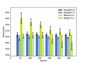
Figure 10: The effect of segmentation on mixing rate.

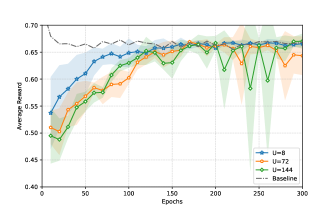
Figure 13: Different communication intervals $U$ under “Merge”.

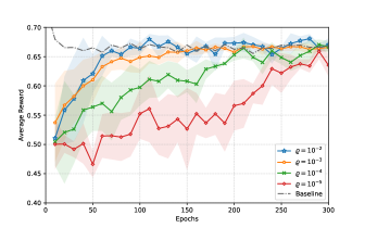
Figure 14: Different target smoothing coefficient $\varrho$ under “Merge”.

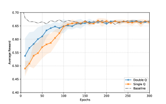
Figure 15: Double vs single $Q$ network under “Merge”.

Beforehand, we present the performance of Independent SAC (ISAC) and Idependent PPO (IPPO) for MARL without any information sharing in Fig. LABEL:fig:IRL, so as to highlight the critical role of inter-agent communication in decentralized cooperative MARL and facilitate subsequent discussions. Fig. LABEL:fig:IRL reveals that the learning process of these non-cooperative algorithms achieves unstable average reward with greater variance, and suffers from the convergence issues even until $300$ epochs. Whereas, when a communication phase involving the exchange of policy parameters is incorporated, as shown in Fig. LABEL:fig:different_method, the learning process within the multi-agent environment is remarkably enhanced in terms of stability and efficiency. In other words, consistent with our previous argument, integrating DFL into IRL significantly improves the training efficiency and ensures the learning stability.

In Fig. LABEL:fig:different_method, we also compare the performance of Regulated Segment Mixture (RSM) and that of the direct, unselective Averaging (Avg) method, as mentioned in Section III. It can be observed in Fig. LABEL:fig:different_method, in terms of convergence speed and stability, the simple average mixture method is somewhat inferior. Particularly in more complex scenario, as in “Merge”, which involves a greater number of RL agents and denser traffic flow compared to the “Figure 8”, the disparity between these two methods becomes more pronounced. The larger variance in the average reward under the average mixture method suggests a more unstable parameter mixing process. Therefore, it validates the effectiveness of RSM and supports the theoretical derived results for selecting useful reference policies and assigning appropriate mixing weights.

On the other hand, Fig. LABEL:fig:different_method further evaluates the performance of RSM on both MASAC and MAPPO. In particular, proposed in our previous work [1], RSM-MAPPO utilizes PPO under traditional RL framework as the independent local updates algorithm, and can be regarded as a special case with $\alpha=0$ as well as different policy advantage estimation. Evidently, in both scenarios, the SAC-based algorithm converges faster and performs better overall compared to the PPO-based algorithm under the same learning rate setting. We believe this is primarily attributed to the differences in exploration mechanism and sample efficiency. Specifically, benefiting from the introduced entropy item under MERL framework, SAC encourages policies to better explore environments, thus capably avoiding local optima and potentially learning faster.

Next, we evaluate the impact of segmentation on the performance, and present the results in Fig. 10. Besides better utilizing the available bandwidth as discussed in Section IV-B, Fig. 10 shows that the incorporation of segmentation (i.e., $P=4$) also leads to an improvement in the successful mixing rate $\rho_{\text{r}}$ of the policy. The improvement lies the introduction of a certain level of randomness, consistent with the idea of entropy encouraged exploration in MERL. Interestingly, the differences in the mixing rate are more pronounced in the more complex “Merge” scenario. Hence, due to the space limitation, we primarily focus on the “Merge” scenario for subsequent discussions.

In Fig. LABEL:fig:Boxplot, we further discuss the effects of the number of segments $P$ and replicas $\kappa$ under RSM-MASAC. Considering that RSM-MASAC generally converges from $250$ to $300$ testing epochs, the results in the boxplots of Fig. LABEL:fig:Boxplot are derived from testing epochs ranging from $150$ to $250$, during which RSM-MASAC experiences more fluctuation and slower convergence, so as to better illustrate the performance during training. Specifically, Fig. LABEL:fig:Boxplot(a) displays the distribution of average reward, where each box represents the InterQuartile Range (IQR). The lower and upper edges of each box denote the first and third quartiles, respectively. Besides, the line inside the box signifies the median average reward for each segment number. Observing Fig. LABEL:fig:Boxplot(a), a trend emerges showing that the median average reward subtly increases with the growing number of segments. Besides, Fig. LABEL:fig:Boxplot(b) shows the median average reward slightly increases along with larger $\kappa$ values, suggesting a trend that more replicas may produce with a higher reward or a higher probability of exploring a better policy, at some cost of a heavier perturbation of the learning process.

In addition, we take the average reward within $250-300$ testing epochs as the final converged performance, and summarize corresponding experimental results and details about communication overhead in Table V. We can find that with $P$ increasing, the mixing rate $\rho_{r}$ also increases first, but slightly decreases when $P=6$, since the aggregation target of reconstructed policy parameters for an over-large $P$ might be mottled and lose the integrity. Besides, a larger $\kappa$ gives the increase of the communication overhead $\psi$, while the final performance gains, especially for $\kappa=5$, $\kappa=7$, are limited, due to that the algorithm has converged to a relative good policy as in centralized FMARL [13].

Furthermore, we also discuss the impact of communication intervals on the learning process, as shown in Fig. 13. It is evident that larger communication intervals result in reduced learning speeds and significant instability in the learning process.

In addition, we conduct more ablation studies to evaluate the design of $Q$ network on the learning process. In Fig. 14, we analyze the impact of different target smoothing coefficients $\varrho$ on the learning process. It can be observed that a larger value of the target smoothing coefficient, such as $10^{-2}$, can significantly accelerate the learning, but it also introduces disturbances, leading to non-steady learning. On the other hand, a smaller value like $10^{-4}$ or $10^{-5}$ noticeably slows down the learning speed, affecting the performance of the algorithm. Hence, we take $\varrho=10^{-3}$ as the default value. Moreover, in Fig. 15, we also evaluate the adoption of dual $Q$ networks. It can be observed that employing dual $Q$ networks indeed accelerates the learning process.

VI Conclusions

In this paper, we have proposed a communication-efficient algorithm RSM-MASAC as a promising solution to enhance communication efficiency and policy collaboration in distributed MARL, particularly in the context of dynamic IoV environments. By delving into the policy parameter mixture function, RSM-MASAC has provided a novel means to leverage and boost the effectiveness of distributed multi-agent collaboration. In particular, RSM-MASAC has successfully transformed the classical means of complete parameter exchange into segment-based request and response, which significantly facilitates the construction of multiple referential polices and simultaneously captures enhanced learning diversity. Moreover, in order to avoid performance-harmful parameter mixture, RSM-MASAC has leveraged a theory-established regulated mixture metric, and selects the contributive referential policies with positive relative policy advantage only. Finally, extensive simulations in the mixed-autonomy traffic control scenarios have demonstrated the effectiveness of the proposed approach.

Appendix: Proofs

VI-A Proof of Soft Policy Improvement

Lemma 1.

(Soft policy improvement) Let $\pi_{\text{old}}$ and $\pi_{\text{new}}$ be the optimizer of the minimization problem defined in (5). Then $Q^{\pi_{\text{new}}}(s,a)\geq Q^{\pi_{\text{old}}}(s,a),\forall s,a$ with $|\mathcal{A}|<\infty$.

Proof.

This proof is a direct application of soft policy improvement [27, 28]. We leave the proof here for completeness.

Let $\pi_{\text{old}}\in\Pi$ and $Q^{\pi},V^{\pi}$ is the corresponding soft state-action value and soft state value, respectively. And $\pi_{\text{new}}$ is defined as:

$$\pi_{\mathrm{new}} =\arg\min_{\pi\in\prod}\mathrm{D}_{\mathrm{KL}}\left(\pi(\cdot|s)\|\frac{\exp\left(\frac{1}{\alpha}Q^{\pi_{\text{old}}}({s},\cdot)\right)}{Z^{\pi_{\text{old}}}(s)}\right)$$

$$=\arg\min_{\pi\in\prod}J_{\pi_{\text{old}}}(\pi(\cdot|s))$$

Since we can always choose $\pi_{\text{new}}=\pi_{\text{old}}\in\Pi$, there must be $J_{\pi_{\text{old}}}(\pi_{\text{new}}(\cdot|s))\leq J_{\pi_{\text{old}}}(\pi_{\text{old}}(\cdot|s))$. Hence

$$\mathbb{E}_{{a}\sim{\pi_{\mathrm{new}}}}\left[\frac{1}{\alpha}Q^{\pi_{\text{old}}}({s},{a})-\log\pi_{\text{new}}(a|s)-\log Z^{\pi_{\text{old}}}(s)\right]$$

$$\geq\mathbb{E}_{{a}\sim\pi_{\text{old}}}\left[\frac{1}{\alpha}Q^{\pi_{\text{old}}}({s},{a})-\log\pi_{\text{old}}(a|s)-\log Z^{\pi_{\text{old}}}(s)\right]$$

as partition function $Z$ depends only on the state, the inequality reduces to a form of the sum of entropy and value with one-step look-ahead

$$\mathbb{E}_{{a}\sim{\pi_{\mathrm{new}}}} \left[Q^{\pi_{\text{old}}}({s},{a})\right]+\alpha H({\pi_{\mathrm{new}}}(\cdot|{s}))$$

$$\geq\mathbb{E}_{{a}\sim\pi_{\text{old}}}\left[Q^{\pi_{\text{old}}}({s},{a})\right]+\alpha H(\pi_{\text{old}}(\cdot|{s}))=V_{\pi_{\text{old}}}(s)$$

And according to the definition of the soft $Q$-value in section II, we can get that

$$Q^{\pi_{\text{old}}}(s,a)$$

$$= \mathop{\mathbb{E}}_{\begin{subarray}{c}s_{1}\end{subarray}}\left[r_{0}\!+\!\gamma\!\left(\!\alpha H(\pi_{\text{old}}(\cdot|s_{1}))\!+\!\!\mathop{\mathbb{E}}_{\begin{subarray}{c}a_{1}\sim\pi_{\text{old}}\end{subarray}}[Q^{\pi_{\text{old}}}(s_{1},a_{1})]\!\right)\!\right]$$ (21)

$$\leq \mathop{\mathbb{E}}_{\begin{subarray}{c}s_{1}\end{subarray}}\left[r_{0}\!+\!\gamma\!\left(\!\alpha H({\pi_{\text{new}}}(\cdot|s_{1}))\!+\!\mathop{\mathbb{E}}_{\begin{subarray}{c}a_{1}\sim{\pi_{\text{new}}}\end{subarray}}[Q^{\pi_{\text{old}}}(s_{1},a_{1})]\!\right)\!\right]$$

$$= \mathop{\mathbb{E}}_{\begin{subarray}{c}s_{1}\\ a_{1}\sim{\pi_{\text{new}}}\end{subarray}}\Big{[}r_{0}+\gamma\left(\alpha H({\pi_{\text{new}}}(\cdot|s_{1}))+r_{1}\right)\Big{]}$$

$$\quad+\gamma^{2}\mathop{\mathbb{E}}_{\begin{subarray}{c}s_{2}\end{subarray}}\left[\alpha H(\pi_{\text{old}}(\cdot|s_{2}))+\mathop{\mathbb{E}}_{\begin{subarray}{c}a_{2}\sim\pi_{\text{old}}\end{subarray}}[Q^{\pi_{\text{old}}}(s_{2},a_{2})]\right]$$

$$\leq \mathop{\mathbb{E}}_{\begin{subarray}{c}s_{1}\\ a_{1}\sim{\pi_{\text{new}}}\end{subarray}}\left[r_{0}+\gamma\left(\alpha H({\pi_{\text{new}}}(\cdot|s_{1}))+r_{1}\right)\right]$$

$$\quad+\gamma^{2}\mathop{\mathbb{E}}_{\begin{subarray}{c}s_{2}\end{subarray}}\left[\alpha H({\pi_{\text{new}}}(\cdot|s_{2}))+\mathop{\mathbb{E}}_{\begin{subarray}{c}a_{2}\sim{\pi_{\text{new}}}\end{subarray}}[Q^{\pi_{\text{old}}}(s_{2},a_{2})]\right]$$

$$= \!\mathop{\mathbb{E}}_{\begin{subarray}{c}s_{1}\\ a_{1}\sim{\pi_{\text{new}}}\\ s_{2}\end{subarray}}\!\!\left[r_{0}\!+\!\gamma\!\left(\alpha H({\pi_{\text{new}}}(\cdot|s_{1}))\!+\!r_{1}\right)\!+\!\gamma^{2}\!\left(\alpha H({\pi_{\text{new}}}(\cdot|s_{2}))\!+\!r_{2}\right)\right]$$

$$\quad+\gamma^{3}\mathop{\mathbb{E}}_{\begin{subarray}{c}s_{3}\end{subarray}}\left[\alpha H({\pi_{\text{new}}}(\cdot|s_{3}))+\mathop{\mathbb{E}}_{\begin{subarray}{c}a_{3}\sim{\pi_{\text{new}}}\end{subarray}}[Q^{\pi_{\text{old}}}(s_{3},a_{3})]\right]$$

$$\quad\cdots$$

$$\leq \mathop{\mathbb{E}}\limits_{\tau_{1}\sim\pi_{\text{new}}}\left[r_{0}+\sum_{t=1}^{\infty}\gamma^{t}\big{(}H({\pi_{\text{new}}}(\cdot|s_{t}))+r_{t}\big{)}\right]$$

$$= Q^{\pi_{\text{new}}}(s,a)$$

∎

VI-B Proof of Theorem 1

Before proving the theorem, we first introduce several important lemmas, on which the proofs of the proposed theorems are built.

Lemma 2.

$$\mathbb{E}_{a\sim\pi}\left[A_{\pi}(s,a)\right]=-\alpha H(\pi(\cdot|s))$$

Proof.

$$\mathbb{E}_{a\sim\pi}\left[A_{\pi}(s,a)\right]$$

$$= \sum_{a}\pi(a|s)A_{\pi}(s,a)$$

$$= \sum_{a}\pi(a|s)\left[Q_{\pi}(s,a)-V_{\pi}(s)\right]$$

$$= \sum_{a}\pi(a|s)Q_{\pi}(s,a)-V_{\pi}(s)$$

$$\stackrel{{\scriptstyle\mathrm{(a)}}}{{=}} \sum_{a}\pi(a|s)Q_{\pi}(s,a)-\sum_{a}\pi(a|s)\left[Q_{\pi}(s,a)-\alpha\log\pi(a|s)\right]$$

$$= -\alpha H(\pi(\cdot|s))$$

where the equality $(a)$ is according to (4). ∎

Lemma 3.

$$\mathop{\mathbb{E}}\limits_{a\sim\pi_{\text{mix}}}\left[A_{\pi}(s,a)\right]=\beta\mathop{\mathbb{E}}\limits_{a\sim\tilde{\pi}}\left[A_{\pi}(s,a)\right]-(1-\beta)\alpha H(\pi(\cdot|s))$$

Proof.

$$\mathbb{E}_{a\sim\pi_{\text{mix}}}\left[A_{\pi}(s,a)\right]$$

$$= \sum_{a}\pi_{\text{mix}}(a|s)A_{\pi}(s,a)$$

$$\stackrel{{\scriptstyle\mathrm{(a)}}}{{=}} \sum_{a}\left[(1-\beta)\pi(a|s)+\beta\tilde{\pi}(a|s)\right]A_{\pi}(s,a)$$

$$= \beta\sum_{a}\tilde{\pi}(a|s)A_{\pi}(s,a)+(1-\beta)\sum_{a}{\pi}(a|s)A_{\pi}(s,a)$$

$$\stackrel{{\scriptstyle\mathrm{(b)}}}{{=}} \beta\mathop{\mathbb{E}}\limits_{a\sim\tilde{\pi}}\left[A_{\pi}(s,a)\right]-(1-\beta)\alpha H(\pi(\cdot|s))$$

where the equalities $(a)$ and $(b)$ are due to (14) and Lemma 2, respectively. ∎

Lemma 4.

For any given state $s$, we can decompose the entropy of the mixed policy as

$$H(\pi_{\text{mix}}(\cdot|s)) =\mathrm{D}_{\mathrm{JS}}^{\beta}(\tilde{\pi}(\cdot|s)\|\pi(\cdot|s))+\beta H(\tilde{\pi}(\cdot|s))$$

$$\qquad+(1-\beta)H(\pi(\cdot|s))$$

Proof.

By definition,

$$H(\pi_{\text{mix}}(\cdot|s))$$

$$= -\sum_{a}\Big{\{}[(1-\beta)\pi(a|s)+\beta\tilde{\pi}(a|s)]$$

$$\qquad\qquad\cdot\log[(1-\beta)\pi(a|s)+\beta\tilde{\pi}(a|s)]\Big{\}}$$

$$= \sum_{a}\beta\left[\tilde{\pi}(a|s)\log\frac{\tilde{\pi}(a|s)}{(1-\beta)\pi(a|s)+\beta\tilde{\pi}(a|s)}\right]$$

$$\quad+\sum_{a}(1-\beta)\left[{\pi}(a|s)\log\frac{{\pi}(a|s)}{(1-\beta)\pi(a|s)+\beta\tilde{\pi}(a|s)}\right]$$

$$\quad-\sum_{a}\left[\beta\tilde{\pi}(a|s)\log\tilde{\pi}(a|s)\right]$$

$$\quad-\sum_{a}\left[(1-\beta){\pi}(a|s)\log{\pi}(a|s)\right]$$

$$= \mathrm{D}_{\mathrm{JS}}^{\beta}(\tilde{\pi}(\cdot|s)\|\pi(\cdot|s))+\beta H(\tilde{\pi}(\cdot|s))+(1-\beta)H(\pi(\cdot|s))$$

∎

Lemma 5.

$$\eta(\pi_{\text{mix}})-\eta(\pi)$$

$$= \sum_{t=0}^{\infty}\gamma^{t}\left[\mathbb{E}_{\begin{subarray}{c}s\sim P(s_{t};\pi_{\text{mix}})\\ a\sim\pi_{\text{mix}}\end{subarray}}[A_{\pi}(s,a)+\alpha H(\pi_{\text{mix}}(\cdot|s))]\right]$$

Proof.

First note that according to the definition of advantage function and soft bellman equation in (2) and (4), we can get $A_{\pi}(s_{t},a_{t})=\mathbb{E}_{s_{t+1}\sim P(\cdot|s_{t},a_{t})}[r_{t}+\gamma V_{\pi}(s_{t+1})-V_{\pi}(s_{t})]$. Therefore,

$$\mathop{\mathbb{E}}\limits_{\tau_{0}\sim\pi_{\text{mix}}}\left[\sum_{t=0}^{\infty}\gamma^{t}\left[A_{\pi}(s_{t},a_{t})\right]\right]$$

$$= \mathop{\mathbb{E}}\limits_{\tau_{0}\sim\pi_{\text{mix}}}\left[\sum_{t=0}^{\infty}\gamma^{t}\left[r_{t}+\gamma V_{\pi}(s_{t+1})-V_{\pi}(s_{t})\right]\right]$$

$$= \mathop{\mathbb{E}}\limits_{\tau_{0}\sim\pi_{\text{mix}}}\Bigg{[}\sum_{t=0}^{\infty}\gamma^{t}r_{t}+(\gamma V_{\pi}(s_{1})-V_{\pi}(s_{0})$$

$$\quad\quad+\gamma^{2}V_{\pi}(s_{2})-\gamma V_{\pi}(s_{1})+\cdots)\Bigg{]}$$

$$= \mathbb{E}_{\tau_{0}\sim\pi_{\text{mix}}}\left[\sum_{t=0}^{\infty}\gamma^{t}r_{t}\right]-\mathbb{E}_{s_{0}}\left[V_{\pi}(s_{0})\right]$$

$${=} \mathbb{E}_{\tau_{0}\sim\pi_{\text{mix}}}\left[\sum_{t=0}^{\infty}\gamma^{t}(r_{t}+\alpha H(\pi_{\text{mix}}(\cdot|s_{t}))\right.$$

$$\quad\left.-\sum_{t=0}\gamma^{t}[\alpha H(\pi_{\text{mix}}(\cdot|s_{t}))]\right]-\eta(\pi)$$

$$= \eta(\pi_{\text{mix}})-\eta(\pi)-\mathbb{E}_{\tau_{0}\sim\pi_{\text{mix}}}\left[\sum_{t=0}^{\infty}\gamma^{t}[\alpha H(\pi_{\text{mix}}(\cdot|s_{t}))]\right]$$

Also we have

$$\mathop{\mathbb{E}}\limits_{\tau_{0}\sim\pi_{\text{mix}}}\left[\sum_{t=0}^{\infty}\gamma^{t}\left[A_{\pi}(s_{t},a_{t})+\alpha H(\pi_{\text{mix}}(\cdot|s_{t}))\right]\right]$$

$$= \sum_{t=0}^{\infty}\gamma^{t}\left[\mathbb{E}_{\begin{subarray}{c}s\sim P(s_{t};\pi_{\text{mix}})\\ a\sim\pi_{\text{mix}}\end{subarray}}[A_{\pi}(s,a)+\alpha H(\pi_{\text{mix}}(\cdot|s))]\right]$$

Hence we can derive the formula for Lemma 5. ∎

Lemma 6.

$$\mathop{\mathbb{E}}_{\begin{subarray}{c}{s\sim P(s_{t};\pi_{\text{mix}})}\\ {a\sim\pi_{\text{mix}}}\end{subarray}}\left[A_{\pi}(s,a)+\alpha H(\pi_{\text{mix}}(\cdot|s))\right]$$

$$\geq \quad\beta\mathop{\mathbb{E}}_{\begin{subarray}{c}s\sim P(s_{t};\pi)\\ a\sim\tilde{\pi}\end{subarray}}\left[A_{\pi}(s,a)+\alpha H(\tilde{\pi}(\cdot|s))\right]-2\beta\rho_{t}\varepsilon$$

$$\quad+\alpha\mathop{\mathbb{E}}\limits_{s\sim P(s_{t};\pi_{\text{mix}})}\left[D_{\text{JS}}^{\beta}(\tilde{\pi}(\cdot|s)\|\pi(\cdot|s))\right]$$

where $\varepsilon=\max_{s}|\mathbb{E}_{a\sim\tilde{\pi}}[A_{\pi}(s,a)+\alpha H(\tilde{\pi}(\cdot|s))]|$, and $\rho_{t}=1-(1-\beta)^{t}$.

Proof.

$$\mathop{\mathbb{E}}_{\begin{subarray}{c}{s\sim P(s_{t};\pi_{\text{mix}})}\\ {a\sim\pi_{\text{mix}}}\end{subarray}}\left[A_{\pi}(s,a)+\alpha H(\pi_{\text{mix}}(\cdot|s))\right]$$

$$\stackrel{{\scriptstyle\mathrm{(a)}}}{{=}}\mathop{\mathbb{E}}\limits_{s\sim P(s_{t};\pi_{\text{mix}})}\Bigg{[}\beta\sum_{a}\tilde{\pi}(a|s)A_{\pi}(s,a)-(1-\beta)\alpha H(\pi(\cdot|s))$$

$$\quad+\alpha\mathrm{D}_{\mathrm{JS}}^{\beta}(\tilde{\pi}(\cdot|s)\|\pi(\cdot|s))\!+\!\beta\alpha H(\tilde{\pi}(\cdot|s))\!+\!(1\!-\!\beta)\alpha H(\pi(\cdot|s))\Bigg{]}$$

$$=\beta\mathop{\mathbb{E}}\limits_{s\sim P(s_{t};\pi_{\text{mix}})}\left[\sum_{a}\tilde{\pi}(a|s)\Big{[}A_{\pi}(s,a)+\alpha H(\tilde{\pi}(\cdot|s))\Big{]}\right]$$

$$\quad+\alpha\mathop{\mathbb{E}}\limits_{s\sim P(s_{t};\pi_{\text{mix}})}\left[\mathrm{D}_{\mathrm{JS}}^{\beta}(\tilde{\pi}(\cdot|s)\|\pi(\cdot|s))\right]$$

where the equality $(a)$ is according to Lemma 3 and Lemma 4, and the mixed policy is taken as a mixture of the policy $\pi$ and the referential policy $\tilde{\pi}$ received from others. In other words, to sample from $\pi_{\text{mix}}$, we first draw a Bernoulli random variable, which tells us to choose $\pi$ with probability $(1-\beta)$ and choose $\tilde{\pi}$ with probability $\beta$. Let $c_{t}$ be the random variable that indicates the number of times $\tilde{\pi}$ was chosen before time $t$. $P(s_{t};\pi)$ is the distribution over states at time $t$ while following $\pi$. We can condition on the value of $c_{t}$ to break the probability distribution into two pieces, with $P(c_{t}=0)=(1-\beta)^{t}$, and $\rho_{t}=P(c_{t}\geq 1)=1-(1-\beta)^{t}$. Thus, we can get (22) on Page 22.

$$\beta\mathop{\mathbb{E}}\limits_{s\sim P(s_{t};\pi_{\text{mix}})}\left[\sum_{a}\tilde{\pi}(a|s)\left[A_{\pi}(s,a)+\alpha H(\tilde{\pi}(\cdot|s))\right]\right]$$

$$= \beta(1-\rho_{t})\!\mathop{\mathbb{E}}\limits_{s\sim P(s_{t}|c_{t}=0;\pi_{\text{mix}})}\!\left[\sum_{a}\tilde{\pi}(a|s)\left[A_{\pi}(s,a)+\alpha H(\tilde{\pi}(\cdot|s))\right]\right]+\beta\rho_{t}\mathop{\mathbb{E}}\limits_{s\sim P(s_{t}|c_{t}\geq 1;\pi_{\text{mix}})}\left[\sum_{a}\tilde{\pi}(a|s)\left[A_{\pi}(s,a)+\alpha H(\tilde{\pi}(\cdot|s))\right]\right]$$

$$= \beta\!\mathop{\mathbb{E}}\limits_{s\sim P(s_{t}|c_{t}=0;\pi_{\text{mix}})}\!\left[\sum_{a}\tilde{\pi}(a|s)\left[A_{\pi}(s,a)+\alpha H(\tilde{\pi}(\cdot|s))\right]\right]-\beta\rho_{t}\mathop{\mathbb{E}}\limits_{s\sim P(s_{t}|c_{t}=0;\pi_{\text{mix}})}\left[\sum_{a}\tilde{\pi}(a|s)\left[A_{\pi}(s,a)+\alpha H(\tilde{\pi}(\cdot|s))\right]\right]$$ (22)

$$\quad+\beta\rho_{t}\mathop{\mathbb{E}}\limits_{s\sim P(s_{t}|c_{t}\geq 1;\pi_{\text{mix}})}\left[\sum_{a}\tilde{\pi}(a|s)\left[A_{\pi}(s,a)+\alpha H(\tilde{\pi}(\cdot|s))\right]\right]$$

Recalling the definition $\varepsilon=\max_{s}\big{|}\mathbb{E}_{a\sim\tilde{\pi}}[A_{\pi}(s,a)+\alpha H(\tilde{\pi}(\cdot|s))]\big{|}$, we have

$$\mathop{\mathbb{E}}\limits_{s\sim P(s_{t}|c_{t}=0;\pi_{\text{mix}})}\left[\sum_{a}\tilde{\pi}(a|s)\left[A_{\pi}(s,a)+\alpha H(\tilde{\pi}(\cdot|s))\right]\right]\leq\varepsilon$$

$$\mathop{\mathbb{E}}\limits_{s\sim P(s_{t}|c_{t}\geq 1;\pi_{\text{mix}})}\left[\sum_{a}\tilde{\pi}(a|s)\left[A_{\pi}(s,a)+\alpha H(\tilde{\pi}(\cdot|s))\right]\right]\geq-\varepsilon$$

Therefore, (22) can be re-organized as

$$\beta\mathop{\mathbb{E}}\limits_{s\sim P(s_{t};\pi_{\text{mix}})}\left[\sum_{a}\tilde{\pi}(a|s)\left[A_{\pi}(s,a)+\alpha H(\tilde{\pi}(\cdot|s))\right]\right]$$

$$\geq \beta\!\mathop{\mathbb{E}}\limits_{s\sim P(s_{t}|c_{t}=0;\pi_{\text{mix}})}\!\left[\sum_{a}\tilde{\pi}(a|s)\left[A_{\pi}(s,a)+\alpha H(\tilde{\pi}(\cdot|s))\right]\right]$$

$$\quad-2\beta\rho_{t}\varepsilon$$

$$= \beta\!\mathop{\mathbb{E}}\limits_{s\sim P(s_{t};\pi)}\!\left[\sum_{a}\tilde{\pi}(a|s)\left[A_{\pi}(s,a)+\alpha H(\tilde{\pi}(\cdot|s))\right]\right]\!-\!2\beta\rho_{t}\varepsilon$$

in which ${P(s_{t}|c_{t}=0;\pi_{\text{mix}})}={P(s_{t};\pi)}$. ∎

Next, we are ready to prove Theorem 1.

Proof.

According to Lemma 5 and Lemma 6, we have

$$\eta(\pi_{\text{mix}})-\eta(\pi)$$

$$= \sum_{t=0}^{\infty}\gamma^{t}\left[\mathbb{E}_{\begin{subarray}{c}s\sim P(s_{t};\pi_{\text{mix}})\\ a\sim\pi_{\text{mix}}\end{subarray}}[A_{\pi}(s,a)+\alpha H(\pi_{\text{mix}}(\cdot|s))]\right]$$

$$\geq \beta\sum_{t=0}^{\infty}\gamma^{t}\!\mathop{\mathbb{E}}_{\begin{subarray}{c}s\sim P(s_{t};\pi)\\ a\sim\tilde{\pi}\end{subarray}}\left[A_{\pi}(s,a)+\alpha H(\tilde{\pi}(\cdot|s))\right]-2\beta\varepsilon\sum_{t=0}^{\infty}\gamma^{t}\rho_{t}$$

$$\quad+\alpha\sum_{t=0}^{\infty}\gamma^{t}\mathop{\mathbb{E}}\limits_{s\sim P(s_{t};\pi_{\text{mix}})}\left[\mathrm{D}_{\mathrm{JS}}^{\beta}(\tilde{\pi}(\cdot|s)\|\pi(\cdot|s))\right]$$

$$= \beta\mathop{\mathbb{E}}_{\begin{subarray}{c}s\sim d_{\pi}\\ a\sim\tilde{\pi}\end{subarray}}\left[A_{\pi}(s,a)+\alpha H(\tilde{\pi}(\cdot|s))\right]-2\beta\varepsilon\sum_{t=0}\gamma^{t}[1-(1-\beta)^{t}]$$

$$\quad+\alpha\mathop{\mathbb{E}}_{s\sim d_{\pi_{\text{mix}}}}\left[\mathrm{D}_{\mathrm{JS}}^{\beta}(\tilde{\pi}(\cdot|s)\|\pi(\cdot|s))\right]$$

$$= \beta\mathop{\mathbb{E}}_{\begin{subarray}{c}s\sim d_{\pi}\\ a\sim\tilde{\pi}\end{subarray}}\left[A_{\pi}(s,a)+\alpha H(\tilde{\pi}(\cdot|s))\right]-\frac{2\gamma\varepsilon\beta^{2}}{(1\!-\!\gamma)(1\!-\!\gamma(1-\beta))}$$

$$\quad+\alpha\mathop{\mathbb{E}}_{s\sim d_{\pi_{\text{mix}}}}\left[\mathrm{D}_{\mathrm{JS}}^{\beta}(\tilde{\pi}(\cdot|s)\|\pi(\cdot|s))\right]$$

$$\geq \beta\mathop{\mathbb{E}}_{\begin{subarray}{c}s\sim d_{\pi}\\ a\sim\tilde{\pi}\end{subarray}}\left[A_{\pi}(s,a)+\alpha H(\tilde{\pi}(\cdot|s))\right]-\frac{2\gamma\varepsilon\beta^{2}}{(1-\gamma)^{2}}$$

$$\quad+\alpha\mathop{\mathbb{E}}_{s\sim d_{\pi_{\text{mix}}}}\left[\mathrm{D}_{\mathrm{JS}}^{\beta}(\tilde{\pi}(\cdot|s)\|\pi(\cdot|s))\right]$$

We have the theorem. ∎

VI-C Derivation of (19)

Lemma 7.

$$\mathbb{A}^{+}_{\pi}(\tilde{\pi}) \approx\mathbb{E}_{s_{t},a_{t}\sim\mathcal{D}}\bigg{[}\left(\frac{\tilde{\pi}_{\tilde{\theta}}(a_{t}|s_{t})-\pi_{\theta}(a_{t}|s_{t})}{\pi_{t}(a_{t}|s_{t})}\right)\!\mathop{\min}_{\begin{subarray}{c}x\in 1,2\end{subarray}}Q_{\omega_{x}}({s}_{t},{a}_{t})$$

$$\qquad+\alpha[H(\tilde{\pi}_{\tilde{\theta}}(\cdot|s_{t}))-H({\pi}_{{\theta}}(\cdot|s_{t}))]\bigg{]}$$

Proof.

Following the definition of policy advantage in (16)

$$\mathbb{A}^{+}_{\pi}(\tilde{\pi})$$

$$= \mathop{\mathbb{E}}_{\begin{subarray}{c}s\sim d_{\pi},a\sim\tilde{\pi}\end{subarray}}\left[A_{\pi}(s,a)+\alpha H(\tilde{\pi}(\cdot|s))\right]$$

$$\stackrel{{\scriptstyle\mathrm{(a)}}}{{=}} \mathop{\mathbb{E}}_{\begin{subarray}{c}s\sim d_{\pi}\end{subarray}}\left[\sum_{a}\tilde{\pi}(a|s)Q^{\pi}(s,a)-V^{\pi}(s)+\alpha H(\tilde{\pi}(\cdot|s))\right]$$

$$\stackrel{{\scriptstyle\mathrm{(b)}}}{{=}} \mathop{\mathbb{E}}_{\begin{subarray}{c}s\sim d_{\pi}\end{subarray}}\Big{[}\sum_{a}\tilde{\pi}(a|s)Q^{\pi}(s,a)-\sum_{a}{\pi}(a|s)Q^{\pi}(s,a)$$

$$\quad-\alpha H({\pi}(\cdot|s))+\alpha H(\tilde{\pi}(\cdot|s))\Big{]}$$

where the equality $(a)$ is according to the state-action advantage value in (2) while $(b)$ follows from (4). Finally, by using Monte Carlo and importance sampling, we can get the lemma.

∎

References

- [1] X. Yu, et al., “Communication-efficient cooperative multi-agent PPO via regulated segment mixture in internet of vehicles,” in Proc. IEEE Globecom 2023, Kuala Lumpur, Malaysia, Dec. 2023.
- [2] Y. Wu, et al., “Deep reinforcement learning on autonomous driving policy with auxiliary critic network,” IEEE Trans. Neural Networks Learn. Sys., vol. 34, no. 7, pp. 3680–3690, Jul. 2023.
- [3] B. R. Kiran, et al., “Deep Reinforcement Learning for Autonomous Driving: A Survey,” IEEE Trans. Intell. Transp. Syst., vol. 23, no. 6, pp. 4909–4926, Jun. 2022.
- [4] A. R. Kreidieh, et al., “Dissipating stop-and-go waves in closed and open networks via deep reinforcement learning,” in Proc. ITSC, Maui, HI, United States, Nov. 2018.
- [5] T. Shi, et al., “Efficient connected and automated driving system with multi-agent graph reinforcement learning,” arXiv preprint arXiv:2007.02794, 2020.
- [6] R. Lowe, et al., “Multi-agent actor-critic for mixed cooperative-competitive environments,” in Proc. NeurIPS, Long Beach, CA, United states, Dec. 2017.
- [7] C. Yu, et al., “The surprising effectiveness of ppo in cooperative multi-agent games,” in Proc. NeurIPS, New Orleans, LA, United states, Nov. 2022.
- [8] J. Foerster, et al., “Counterfactual multi-agent policy gradients,” in AAAI Conf. Artif. Intell., New Orleans, LA, United states, Feb. 2018.
- [9] J. Foerster, et al., “Learning to communicate with deep multi-agent reinforcement learning,” in Proc. NeurIPS, Barcelona, Spain, Dec. 2016.
- [10] L. Matignon, et al., “Independent reinforcement learners in cooperative markov games: a survey regarding coordination problems,” Knowl. Eng. Rev., vol. 27, no. 1, pp. 1–31, Mar. 2012.
- [11] M. Tan, “Multi-agent reinforcement learning: Independent vs. cooperative agents,” in Proc. ICML, University of Massachusetts, Amherst, Jun. 1993.
- [12] G. Papoudakis, et al., “Benchmarking multi-agent deep reinforcement learning algorithms in cooperative tasks,” arXiv preprint arXiv:2006.07869, 2020.
- [13] X. Xu, et al., “The gradient convergence bound of federated multi-agent reinforcement learning with efficient communication,” IEEE Trans. Wireless Commun., 2023, (accepted), doi: 10.1109/TWC.2023.3279268.
- [14] J. Qi, et al., “Federated reinforcement learning: Techniques, applications, and open challenges,” arXiv preprint arXiv:2108.11887, 2021.
- [15] Z. Xie, et al., “Fedkl: Tackling data heterogeneity in federated reinforcement learning by penalizing kl divergence,” IEEE J. Sel. Areas. Commun., vol. 41, no. 4, pp. 1227–1242, Apr. 2023.
- [16] Y. Fu, et al., “A selective federated reinforcement learning strategy for autonomous driving,” IEEE Trans. Intell. Transp. Syst., vol. 24, no. 2, pp. 1655–1668, Feb. 2023.
- [17] S. Savazzi, et al., “Federated learning with cooperating devices: A consensus approach for massive iot networks,” IEEE Internet Things J., vol. 7, no. 5, pp. 4641–4654, May 2020.
- [18] J. Wang, et al., “Cooperative sgd: A unified framework for the design and analysis of local-update sgd algorithms,” J. Mach. Learn. Res., vol. 22, no. 1, pp. 9709–9758, Sep. 2021.
- [19] W. Liu, et al., “Decentralized federated learning: Balancing communication and computing costs,” IEEE Trans. Signal Inf. Process. Over Netw., vol. 8, pp. 131–143, Feb. 2022.
- [20] T. Sun, et al., “Decentralized federated averaging,” IEEE Trans. Pattern Anal. Mach. Intell., vol. 45, no. 4, pp. 4289–4301, Apr. 2023.
- [21] P. Watcharapichat, et al., “Ako: Decentralised deep learning with partial gradient exchange,” in Proc. ACM Symp. Cloud Comput., SoCC, Santa Clara, CA, United states, Oct. 2016.
- [22] L. Barbieri, et al., “Communication-efficient Distributed Learning in V2X Networks: Parameter Selection and Quantization,” in Proc. IEEE Globecom, Rio de Janeiro, Brazil, Dec. 2022.
- [23] C. Hu, et al., “Decentralized federated learning: A segmented gossip approach,” arXiv preprint arXiv:1908.07782, 2019.
- [24] P. Kairouz, et al., “Advances and open problems in federated learning,” Found. Trends Mach. Learn., vol. 14, no. 1–2, pp. 1–210, Jun. 2021.
- [25] X. Wang, et al., “Federated deep reinforcement learning for internet of things with decentralized cooperative edge caching,” IEEE Internet Things J., vol. 7, no. 10, pp. 9441–9455, Oct. 2020.
- [26] T. Haarnoja, et al., “Reinforcement learning with deep energy-based policies,” in Proc. ICML, Sydney, NSW, Australia, Aug. 2017.
- [27] T. Haarnoja, et al., “Soft actor-critic: Off-policy maximum entropy deep reinforcement learning with a stochastic actor,” in Proc. ICML, Stockholm, Sweden, Jul. 2018.
- [28] T. Haarnoja, et al., “Soft actor-critic algorithms and applications,” arXiv preprint arXiv:1812.05905, 2018.
- [29] P. Dhariwal, et al., “Openai baselines,” 2017.
- [30] C. S. de Witt, et al., “Is independent learning all you need in the starcraft multi-agent challenge?” arXiv preprint arXiv:2011.09533, 2020.
- [31] V. Mnih, et al., “Asynchronous methods for deep reinforcement learning,” in Proc. ICML, New York City, NY, United states, Jun. 2016.
- [32] J. Schulman, et al., “Proximal policy optimization algorithms,” arXiv preprint arXiv:1707.06347, 2017.
- [33] J. Schneider, et al., “Distributed value functions,” in Proc. ICML, Bled, Slovenia, Jun. 1999.
- [34] E. Ferreira, et al., “Multi agent collaboration using distributed value functions,” in Proc. IEEE Intell. Veh. Symp., Dearbon, MI, United states, Oct. 2000.
- [35] W. Liu, et al., “Distributed cooperative reinforcement learning-based traffic signal control that integrates v2x networks’ dynamic clustering,” IEEE Trans. Veh. Technol., vol. 66, no. 10, pp. 8667–8681, Oct. 2017.
- [36] X. Xu, et al., “Stigmergic independent reinforcement learning for multiagent collaboration,” IEEE Trans. Neural Networks Learn. Sys., vol. 33, no. 9, pp. 4285–4299, Sep. 2021.
- [37] G. Sartoretti, et al., “Distributed reinforcement learning for multi-robot decentralized collective construction,” in Springer. Proc. Adv. Robot. Springer, 2019.
- [38] H. Tang, et al., “Communication compression for decentralized training,” in Proc. NeurIPS, Montréal, Canada, Dec. 2018.
- [39] Z. Tang, et al., “Gossipfl: A decentralized federated learning framework with sparsified and adaptive communication,” IEEE Trans. Parallel Distrib. Syst., vol. 34, no. 3, pp. 909–922, Mar. 2023.
- [40] X. Xu, et al., “Trustable Policy Collaboration Scheme for Multi-Agent Stigmergic Reinforcement Learning,” IEEE Commun. Lett., vol. 26, no. 4, pp. 823–827, Apr. 2022.
- [41] S. Kakade, et al., “Approximately optimal approximate reinforcement learning,” in Proc. ICML, Sydney, Australia, Jul. 2002.
- [42] J. Schulman, et al., “Trust region policy optimization,” in Proc. ICML, Lille, France, Jul. 2015.
- [43] J. Kuba, et al., “Trust region policy optimisation in multi-agent reinforcement learning,” in Proc. ICLR, Virtual, Online, Apr. 2022.
- [44] R. Molina-Masegosa, et al., “Lte-v for sidelink 5g v2x vehicular communications: A new 5g technology for short-range vehicle-to-everything communications,” IEEE Veh. Technol. Mag., vol. 12, no. 4, pp. 30–39, Dec. 2017.
- [45] J. Duan, et al., “Distributional soft actor-critic: Off-policy reinforcement learning for addressing value estimation errors,” IEEE Trans. Neural Networks Learn. Sys., vol. 33, no. 11, pp. 6584–6598, Nov. 2021.
- [46] S. Fujimoto, et al., “Addressing function approximation error in actor-critic methods,” in Proc. ICML, Stockholm, Sweden, Jul. 2018.
- [47] I. Hegedűs, et al., “Gossip learning as a decentralized alternative to federated learning,” in 19th IFIP WG 6.1 International Conference on Distributed Applications and Interoperable Systems, Kongens Lyngby, Denmark, Jun. 2019.
- [48] F. Nielsen, “On the jensen–shannon symmetrization of distances relying on abstract means,” Entropy, vol. 21, no. 5, p. 485, May 2019.
- [49] S. M. Kakade, “A natural policy gradient,” Denver, Colorado, United states, Dec. 2001.
- [50] S.-I. Amari, “Natural gradient works efficiently in learning,” Neural Comput., vol. 10, no. 2, pp. 251–276, Feb. 1998.
- [51] T. George, et al., “Fast approximate natural gradient descent in a kronecker factored eigenbasis,” Montreal, QC, Canada, Dec. 2018.
- [52] J. Martens, et al., “Deep learning via hessian-free optimization.” in Proc. ICML, Haifa, Israel, Jun. 2010.
- [53] C. Wu, et al., “Flow: A modular learning framework for mixed autonomy traffic,” IEEE Trans. Rob., vol. 38, no. 2, pp. 1270–1286, Apr. 2022.
- [54] E. Vinitsky, et al., “Benchmarks for reinforcement learning in mixed-autonomy traffic,” in Proc. CoRL, Zürich, Switzerland, Oct. 2018.
- [55] M. Treiber, et al., “Congested traffic states in empirical observations and microscopic simulations,” Physical review E, vol. 62, no. 2, p. 1805, Aug. 2000.
- [56] B. Xiao, et al., “Stochastic graph neural network-based value decomposition for multi-agent reinforcement learning in urban traffic control,” in Proc. IEEE VTC 2023-Spring, Florence, Italy, Jun. 2023.