Robust Estimation of Causal Heteroscedastic Noise Models

Abstract

Distinguishing the cause and effect from bivariate observational data is the foundational problem that finds applications in many scientific disciplines. One solution to this problem is assuming that cause and effect are generated from a structural causal model, enabling identification of the causal direction after estimating the model in each direction. The heteroscedastic noise model is a type of structural causal model where the cause can contribute to both the mean and variance of the noise. Current methods for estimating heteroscedastic noise models choose the Gaussian likelihood as the optimization objective which can be suboptimal and unstable when the data has a non-Gaussian distribution. To address this limitation, we propose a novel approach to estimating this model with Student’s $t$-distribution, which is known for its robustness in accounting for sampling variability with smaller sample sizes and extreme values without significantly altering the overall distribution shape. This adaptability is beneficial for capturing the parameters of the noise distribution in heteroscedastic noise models. Our empirical evaluations demonstrate that our estimators are more robust and achieve better overall performance across synthetic and real benchmarks.

1 Introduction

The aim of the causal discovery is to uncover the underlying causal relationships of the data. This task is relevant in various scientific disciplines such as biology, economics, and sociology [17]. One foundational challenge in causal discovery involves identifying the cause and effect between two variables $X$ and $Y$. Randomized controlled trials (RCT) are considered the ideal solution for determining causal relationships, particularly in medicine [6]. However, RCTs require active intervention in variables and observation of corresponding feedback, making them resource-intensive and sometimes ethically impractical. To overcome the limitations of RCT, studying observational data becomes a more challenging yet necessary approach for identifying causal relationships.

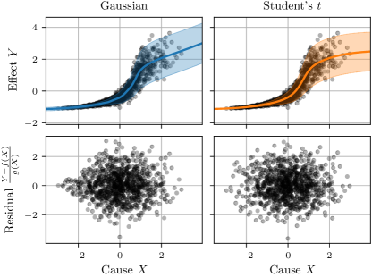
Figure 1: Heteroscedastic noise models estimated with Gaussian distribution and Student’s $t$-distribution for the likelihood $p\left(Y\mid X\right)$ on pair 82 of the LS-s dataset. The Gaussian estimation fails to capture the regions with small sample sizes and low variances, which causes suboptimal fits in these regions. In contrast, estimating with a more robust Student’s $t$-distribution allows the model to better capture the distribution of the noise. Accordingly, our estimation method with $t$-distribution can correctly retrieve the residual $N_{Y}=\frac{Y-f\left(X\right)}{g\left(X\right)}$ that is independent of the cause $X$.

With solely observational data, determining the causal direction between $X$ and $Y$ requires prior assumptions of the data-generating process, which is commonly represented by structural causal models (SCMs) [17]. In general, an SCM includes a cause variable $X$, an independent noise term $N_{Y}$ ($N_{Y}\operatorname{\perp\!\!\!\perp}X$), and an effect variable $Y$ generated from $X$ and $N_{Y}$ via a function $f$. By restricting the formulation of $f$, the identifiability or the ability to identify the causal direction from observational data has been intensively studied. The earliest and the most comprehensively examined model is the branch of additive noise models (ANMs), where the noise term is added after applying the function $f$: $Y:=f\left(X\right)+N_{Y}$. This model is proven to be identifiable when $f$ is linear and $N$ has a non-Gaussian distribution [24] or when $f$ is non-linear [7]. As the cause only affects the mean of the noise, ANMs can be estimated easily and there exist consistent estimators for these models [14]. Post non-linear noise models (PNLs) are more complex than ANMs where an additional non-linear invertible function $g$ is applied after the noise addition: $Y:=g\left(f\left(X\right)+N_{Y}\right)$. Various works have also been conducted to study the identifiability and estimation of PNL models [31, 32]. Heteroscedastic noise models (HNMs) emerge as generalizations of ANMs. In HNMs, the cause appears in not only the additive form but also in the multiplicative form: $Y:=f\left(X\right)+g\left(X\right)N_{Y}$. In addition to identifiability conditions [12, 26, 9], several methods for predicting the causal direction between two variables with HNMs [27, 12, 26, 30, 9] have been proposed.

Current estimators for HNMs use Gaussian likelihood as the optimization objective [9]. The estimation is achieved by modeling the mean $\mu\left(X\right)$ and the variance $\sigma^{2}\left(X\right)$ and maximizing the Gaussian log-likelihood $\log p\left(Y\mid X\right):=\log\mathcal{N}\left(Y\mid\mu\left(X\right),\sigma^{2}\left(X\right)\right)$. Although Gaussian distribution is a common choice for the likelihood, this light-tailed distribution is sensitive to small sample sizes and extreme values. Figure 1 demonstrates an example where a region has a small sample size and low variances, the model fitted with Gaussian likelihood cannot capture the variance correctly. In this study, we propose ROCHE—a RObust estimation approach for Causal HEteroscedastic noise models with Student’s $t$-distribution using neural networks. The $t$-distribution is a heavy-tailed distribution that generalizes the Gaussian distribution with an additional degree of freedom parameter $\nu$. The degree of freedom $\nu$ controls the heaviness of the tails which improves the adaptability of the model estimation without changing the general shape of the distribution significantly. With the robustness in model estimation, our proposed approach achieves better performance on most bivariate causal discovery benchmarks with higher stability compared to models estimated with Gaussian likelihood and other related approaches.

Contributions. The key contributions of this study can be summarized as follows:

1. We propose a robust estimation approach for identifying the causal direction of heteroscedastic noise models with Student’s $t$-distribution. This approach addresses the limitations of using Gaussian likelihood and provides a more robust alternative for modeling the noise distribution.

2. We design a framework that incorporates neural networks to robustly estimate the $t$-distribution likelihood. We introduce essential constraints that are specifically tailored for the bivariate causal discovery task, ensuring accurate and reliable estimation results.

3. We demonstrate the effectiveness of our approach by comparing it with related approaches for both homoscedastic and heteroscedastic noise models. We evaluate our method on 13 commonly used bivariate causal discovery benchmarks, showcasing its superior performance and robustness.

2 Related Works

Although the bivariate causal discovery or cause-effect inference from observational data is fundamental and well-defined, this task still attracts a considerable amount of research attention. Compared to multivariate settings, the bivariate setting is more limited in identifying information such as global information about the causal structures. The recent related literature aiming to infer the cause-effect relationship between two variables can be categorized into three branches which will be presented below.

Methods based on cause-effect asymmetry

The first branch of approaches explores the assumptions of identifiable structural causal models (SCMs), where the causal models in the anti-causal directions are proven to be non-existent. Scores for quantifying this asymmetry in model existence are designed for each type of SCM. Prevalent scoring choices for determining the causal direction are the log-likelihood and non-parametric independent test scores such as the Hilbert-Schmidt Independence Criterion (HSIC) [5] or mutual information between the estimated residual and the cause. Various approaches in this branch has been extended to handle multivariate data. In homoscedastic/additive noise models where the cause only is assumed to contribute only to the means, mean regression methods are being used in many methods for estimating the models [24, 7, 19, 20, 18, 1]. After the estimation step, the maximum likelihood is employed for inferring the cause and effect in CAM [1]. Correspondingly, RESIT [20] also executes the mean estimation, but an additional step of independence testing is performed subsequently.

For heteroscedastic noise models, many works aiming to quantify the asymmetry have been introduced. CAREFL [12] assumes the invertibility of the functions with the Gaussianity of the noises and estimates the models with autoregressive normalizing flows [8]. The likelihood of the affine autoregressive flows is then computed on both training and test data to conclude the cause-effect direction. HECI [30] divides the assumed cause $X$ in the several bins and, in each bin, the model is assumed to have a homoscedastic noise form. The BIC score is computed in each bin, and the correct causal direction is the one that will minimize this score. GRCI [26] regresses the mean and the mean absolute deviation (MAD) with a leave-one-out cross-validation approach. The residual is computed from the estimated mean and MAD, and the independence between the residual and the corresponding cause is assessed by the mutual information. A consistent estimator and a neural network-based estimator for maximizing the Gaussian log-likelihood are presented in LOCI [9]. Besides utilizing the log-likelihood as a criterion, from the mean and the variance parameters of the Gaussian distribution, the residual can be recovered for the next step of testing the independence with HSIC. As our proposed approach belongs to this group, ROCHE follows the same procedure for predicting the causal direction as previous methods.

Methods based on independence between cause and mechanism

The second branch of methods relies on the postulate of the independence between the cause and the mechanism. If the causal direction between $X$ and $Y$ is $X\rightarrow Y$, the marginal distribution of the cause $P\left(X\right)$ is independent of the conditional distribution of the effect given the cause $P\left(Y\mid X\right)$ and not vice versa. IGCI [10] considers the case with low noise levels and formularizes this independence in terms of information geometry for distinguishing the cause and effect with relative entropy distances. CDCI [3] is based on the assumption that the conditional distribution of the effect given the cause is invariant in shape. Another interpretation of this independence in the causal mechanism is the sum of the Kolmogorov complexities [13] of $P_{X}$ and $P_{Y\mid X}$ [11, 15]. The minimum description length (MDL) is adopted for approximating the Kolmogorov complexity as this complexity is not computable. QCCD [27] also follows this interpretation with non-parametric quantile regression and code length computation for distinguishing the cause and effect.

3 Preliminaries

3.1 Heteroscedastic Noise Models & Causal-Effect Inference

(Heteroscedastic Noise Model [9]). Given a random variable $X$ as the cause and a random variable $N_{Y}$ as the noise that is independent to $X$ ($N_{Y}\operatorname{\perp\!\!\!\perp}X$), a heteroscedastic noise model or, in different terms, a location-scale noise model generates the effect variable $Y$ with the following formulation:

(3.1) $$Y:=f\left(X\right)+g\left(X\right)N_{Y},$$

where $f:\mathcal{X}\rightarrow\mathbb{R}$ and $g:\mathcal{X}\rightarrow\mathbb{R}_{+}$.

Without loss of generality, for easier estimation, the mean of the noise $\mathbb{E}\left[N_{Y}\right]$ is assumed to be equal to $0$. The functions $f\left(X\right)$ and $g\left(X\right)$ contribute to the mean and standard deviation of the noise. To estimate $f\left(X\right)$ and $g\left(X\right)$, we can estimate the mean and the standard deviation of $p\left(Y\mid X\right)$. There are two approaches to estimating the noise term $N_{Y}$ in HNM. GRCI [26] uses leave-one-out cross-validation to learn the models for regressing the mean and the mean absolute deviation (MAD). GRCI estimates MAD instead of the standard deviation as the MAD can be estimated directly and have smaller estimation errors. However, the use of cross-validation, especially the leave-one-out method, has high a computational cost. LOCI [9], on the other hand, models the mean and the variance and uses the Gaussian log-likelihood $\log\mathcal{N}\left(Y\mid\mu\left(X\right),\sigma^{2}\left(X\right)\right)$ as the maximization objective. This approach allows the mean and the variance can be optimized simultaneously, but the assumption of the Gaussian likelihood is more restrictive compared to GRCI’s approach.

3.2 Student’s $t$-Distribution

Student’s $t$-distribution is a distribution that is considered as the generalization of Gaussian distribution. Belonging to the location-scale family as the Gaussian family, the $t$-distribution’s parameters also include a location $\mu$ and a scale $\tau^{2}$. In addition to the location and scale, the third parameter of the $t$-distribution is the degree of freedom $\nu$ ($\nu>0$). The probability density function (PDF) of the $t$-distribution in defined as

(3.2) $$t\left(x\mid\mu,\tau^{2},\nu\right)=\frac{\Gamma\left(\frac{\nu+1}{2}\right)}{\Gamma\left(\frac{\nu}{2}\right)\sqrt{\pi\nu\tau^{2}}}\left(1+\frac{1}{\nu}\frac{\left(x-\mu\right)^{2}}{\tau^{2}}\right)^{-\frac{\nu+1}{2}},$$

where $\Gamma\left(z\right)=\int_{0}^{\infty}t^{z-1}\exp\left(-t\right)dt$. As derived from Eq. (3.2), $t$-distribution is a heavy-tailed distribution where the heaviness of the tails is controlled by the degree of freedom $\nu$. As $\nu\rightarrow\infty$, the $t$-distribution will become the Gaussian distribution. If $\nu>1$, the expected value of the random variable $X\sim t\left(\mu,\tau^{2},\nu\right)$ is defined as

(3.3) $$\mathbb{E}\left[X\right]=\mu,$$

and when $\nu>2$, the variance of $X$ is definite and is calculated from both the scale $\tau^{2}$ and the degree of freedom $\nu$ as follows

(3.4) $$\operatorname{Var}\left[X\right]=\tau^{2}\frac{\nu}{\nu-2}.$$

Having an additional parameter $\nu$ controlling the variance allows the $t$-distribution to handle sampling variability and extreme outliers by adapting the shape of the distribution flexibly (see Figure 1 for an example). Therefore, the $t$-distribution is more robust than the Gaussian distribution while maintaining the ability to approximate the Gaussian distribution by using a high degree of freedom. Due to these advantages, this distribution can be applied in place of the Gaussian distribution improve the robustness such as in the Student-$t$ processes [23, 29] as alternatives for Gaussian processes, reliable variance networks estimation [2], or Student-$t$ variational autoencoder [28] for more robust density estimation. Following these intuitions, we choose the $t$-distribution for the likelihood in our approach to achieve a robust estimation of the heteroscedastic noise models.

4 ROCHE: Robust Estimation of Causal Heteroscedastic Noise Models

4.1 Parameters Estimation with the $t$-Distribution

Similar to previous approaches [26, 9], we need to estimate the mean and the standard deviation to retrieve the independent residual. We estimate these parameters via the likelihood of the assumed effect $Y$ given the assumed cause $X$. The $t$-distribution probability density function in Eq. (3.2) is chosen for this likelihood as follows

(4.5) $$p\left(Y\mid X\right)=t\left(Y\mid\mu\left(X\right),\tau^{2}\left(X\right),\nu\left(X\right)\right),$$

and this likelihood is modeled using a neural network. Inspired by the fact that the $t$-distribution is a Gaussian distribution with the variance distributed as an inverse gamma distribution with two parameters $a=\nu/2$ and $b=\nu\tau^{2}/2$. Instead of modeling the scale function $\tau^{2}\left(X\right)$ and the degree of freedom function $\nu\left(X\right)$ separately, we model two alternative parameter functions $a\left(X\right)$ and $b\left(X\right)$. The degree of freedom $\nu$ and the scale $\tau^{2}$ are then computed as

(4.6) $$\nu\left(X\right)=2a\left(X\right),$$

(4.7) $$\tau^{2}\left(X\right)=\frac{b\left(X\right)}{a\left(X\right)}.$$

By doing so, the scale $\tau^{2}$ depends on the degree of freedom $\nu$, and will adapt accordingly to the change in the degree of freedom. Since the degree of freedom must be greater than $2$ for the variance to exist and the scale of the $t$-distribution must be greater than $0$, the constraints $a\left(X\right)>1$ and $b\left(X\right)>0$ are applied when modeling.

With this model, the neural network is optimized by minimizing the negative log-likelihood as the loss function

(4.8) $$\mathcal{L}_{\text{NLL}} =-\frac{1}{n}\sum_{i=1}^{n}\log t\left(y_{i}\mid\mu\left(x_{i}\right),\tau^{2}\left(x_{i}\right),\nu\left(x_{i}\right)\right)$$

where $n$ is the number of samples and $\left(x_{i},y_{i}\right)$ is the $i$-th sample from the dataset. There could be many models that can be fitted with this loss function. The most preferable models are the one with higher degrees of freedom which approach the Gaussian distribution. To implement this preference, in addition to the negative log-likelihood loss, we propose an additional constraint loss for the degree of freedom $\nu\left(\cdot\right)$ as follows

(4.9) $$\mathcal{L}_{\text{constraint}} =\frac{1}{n}\sum_{i=1}^{n}\left(\frac{\nu\left(x_{i}\right)}{\nu\left(x_{i}\right)-2}\right)^{2}$$

This constraint is chosen from the $t$-distribution’s variance in Eq. (3.4), where the variance is scaled from the distribution’s scale parameter $\tau^{2}$ with a factor of $\nu/\left(\nu-2\right)$. The value of the constraint will decrease and approach $1$ when all the values of $\nu\left(x_{i}\right)$ increase. Penalizing this constraint will also reduce the scaling term of the variance in Eq. (3.4), which makes the variance become more stable by having values closer to $\tau^{2}$ instead of exploding to infinity. Moreover, as the parameter $\tau^{2}$ in our approach is modeled with Eq. (4.7), raising the value of $\nu$ which corresponds to $a$ will also decrease the value of $\tau^{2}$. This behavior can avoid the underfitting scenario where the location parameter $\mu$ is poorly predicted but the scale is increased to account for the high error ranges. This scenario also happens to the Gaussian log-likelihood where many approaches, such as $\beta$-NLL [22] or Faithful Heteroscedastic [25], has been proposed to have more reliable mean regression by modifying the Gaussian log-likelihood function, but these methods need to have a trade-off between the mean accuracy and the log-likelihood. We do not have this trade-off since the constraint term is a detached module and our method still tries to find the models with the highest log-likelihood.

4.2 Residual Estimation & Cause-Effect Inference

After estimating heteroscedastic noise models in Eq. (3.1), the residual can be computed from the estimands as follows

(4.10) $$\tilde{N}_{Y}=\frac{Y-\tilde{f}\left(X\right)}{\tilde{g}\left(X\right)},$$

where $\tilde{N}_{Y}$, $\tilde{f}\left(X\right)$ and $\tilde{g}\left(X\right)$ denote the estimated $N_{Y}$, $f\left(X\right)$, and $g\left(X\right)$. In our case with the $t$-distribution, the function $f\left(X\right)$ corresponds to $\mathbb{E}\left[Y\mid X\right]=\mu\left(X\right)$ and $g^{2}\left(X\right)$ corresponds to $\operatorname{Var}\left[Y\mid X\right]=\tau^{2}\left(X\right)\frac{\nu\left(X\right)}{\nu\left(X\right)-2}$. After learning the model, the estimated residual can be determined from the estimated parameters of the $t$-distribution as follows

(4.11) $$\tilde{N}_{Y} =\frac{Y-\tilde{\mu}\left(X\right)}{\sqrt{\tilde{\tau^{2}}\left(X\right)\frac{\tilde{\nu}\left(X\right)}{\tilde{\nu}\left(X\right)-2}}}$$

where $\tilde{\mu}$, $\tilde{\tau^{2}}$, $\tilde{\nu}$, $\tilde{a}$, and $\tilde{b}$ are the parameters estimated with the $t$-distribution likelihood.

As the noise term $N_{Y}$ and the cause $X$ are assumed to be independent, the dependence between the estimated noise $\tilde{N}_{Y}$ and the cause $X$ quantified using any non-parametric independent test can be utilized to support the cause-effect inference step. In previous approaches, GRCI [26] estimates the the independence between $\tilde{N}_{Y}$ and $X$ via the mutual information, whereas LOCI [9] uses the Hilbert-Schmidt independence criterion (HSIC) [5]. The Gaussian log-likelihood is also proposed in LOCI [9] as a score for quantifying the causal direction. However, using Gaussian likelihood scoring can cause model misspecification when the distribution of the noise is non-Gaussian, especially in heteroscedastic noise models [21]. A more suitable choice should be using the quantified dependence between $\tilde{N}_{Y}$ and $X$. In this work, we choose the HSIC score [5] for easier comparison with LOCI [9], which chooses the Gaussian likelihood for estimating the heteroscedastic noise models. Higher HSIC score indicates that two variables have a higher degree of independence.

5 Experiments

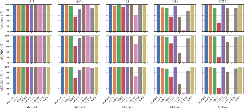
Figure 2: Performance on synthetic additive (AN & AN-s), location-scale (LS & LS-s), and multiplicative (MN-U) noise models. Higher accuracy, AUDRC, and AUROC are preferable. Our ROCHE approach is compared with methods for heteroscedastic noise models: LOCI [9], GRCI [26], HECI [30], and QCCD [27], and methods not designed for heteroscedasticity: CAM [1], RESIT [20], CGNN [4], and ICGI [10]. Our ROCHE approach achieves perfect results on all 5 benchmark datasets.

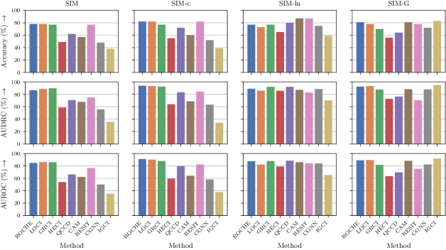
Figure 3: Performance on SIM, SIM-c, SIM-ln, and SIM-G datasets. Higher accuracy, AUDRC, and AUROC are preferable. Our ROCHE approach is compared with methods for heteroscedastic noise models: LOCI [9], GRCI [26], HECI [30], and QCCD [27], and methods not designed for heteroscedasticity: CAM [1], RESIT [20], CGNN [4], and ICGI [10]. ROCHE acquires comparable and stable results on most datasets and accomplishes better results in comparison with the Gaussian-likelihood-based LOCI. Regression-based methods with subsequent independence tests including ROCHE, LOCI, GRCI, and RESIT have better performance in the occurrence of confounders.

5.1 Experimental Settings

In this section, we compare our ROCHE approach with related bivariate causal discovery methods designed for heteroscedastic noise models and homoscedastic noise models to demonstrate the effectiveness of our approach.

Baselines

Evaluated state-of-the-art causal discovery methods for heteroscedastic noise models including QCCD [27], HECI [30], GRCI [26], and LOCI [9]. Among these approaches, the most related method to our approach is LOCI which employs the Gaussian likelihood for estimating the location and scale of the model. For LOCI, we use the neural network version with HSIC as the score for easier comparisons. For methods that are designed for homoscedastic or additive noise models, we use CAM [1] and RESIT [20]. For other baselines that do not assume heteroscedastic noise models, we consider ICGI [10] with Gaussian reference measures and CGNN [4].

Datasets

We use both synthetic and real causal discovery benchmarks to evaluate our approach.

The first group of chosen benchmarks is the five synthetic datasets from [27] including AN, AN-s, LS, LS-s, and MN-U. These five datasets are generated from structural causal models that are heteroscedastic (or location-scale) noise models (LS and LS-s datasets) and special cases of heteroscedastic noise models consisting of homoscedastic additive noise models (AN and AN-s datasets) and multiplicative noise models (MN-U). The datasets denoted with “-s” and the MN-U dataset use invertible sigmoid-type functions for the generative functions which can make the identification of the causal direction more complicated.

In the second group of benchmarks, we consider more difficult synthetic datasets comprising the SIM, SIM-c, SIM-ln, and SIM-G from [16] and the Multi and Net datasets from [4], the Cha dataset from [6]. The four SIM, SIM-c, SIM-ln, SIM-G datasets are simulated with the functions $X:=f_{X}\left(N_{X}\right)$ and $Y:=f_{Y}\left(X,N_{Y}\right)$ in the cases without a confounder (in SIM, SIM-ln, and SIM-G) and the functions $Z:=f_{Z}\left(N_{Z}\right)$, $X:=f_{X}\left(N_{X},N_{Z}\right)$, and $Y:=f_{Y}\left(X,N_{Y},N_{Z}\right)$ in the cases with a confounder $Z$ (in SIM-c). In the SIM-ln dataset, low levels of noise are applied in the models, and the SIM-G dataset has approximations of Gaussian distributions for the cause $X$ and approximately Gaussian non-linear additive noise generative models. The Multi dataset is generated with pre-additive noises ($Y:=f\left(X+N_{Y}\right)$), post-additive noises (similar to conventional additive noise models), pre-multiplicative noise ($Y:=f\left(X\times N_{Y}\right)$), and post-multiplicative noise ($Y:=f\left(X\right)\times N_{Y}$). The pairs in the Net dataset are generated with neural networks with random distribution for $X$, such as exponential, gamma, log-normal, or Laplace distribution. The 300 continuous variable pairs in the Cha benchmark are chosen from the ChaLearn Cause-Effect Pairs Challenge [6].

For a real-world benchmark, we choose the Tübingen cause-effect pairs [16] for comparison. This dataset contains pairs of cause(s) and effect(s) gathered from many sources with diverse domains. Each pair in this benchmark has a corresponding weight to scale down the results of pairs having similar properties. For that reason, the evaluation results for this benchmark are also weighted according to these weights.

Metrics

The cause-effect inference results are assessed with three common metrics in bivariate causal discovery literature consisting of the accuracy score, the area under the decision rate curve (AUDRC), and the area under the receiver operating characteristic curve (AUROC). The accuracy score is the simplest evaluation metric which computes the percentage of the pairs in the datasets whose causal directions are correctly predicted. The AUDRC criterion is proposed in [9] for quantifying the extent to which decision confidence aligns with accuracy. Having higher AUDRC means that the methods will predict the correct causal directions if the confidence of the scores is high, and the incorrect cases are caused by lower confidence of the predicted score. The last chosen metric is the AUROC score. This score indicates the ability of the methods to predict correctly without intermingling between the two causal directions. To compensate for the class imbalance when computing the AUROC score, we augment the results by adding an additional result for the reversed direction with a reversed label for each result acquired.

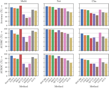
Figure 4: Performance on Multi, Net, and Cha datasets. Higher accuracy, AUDRC, and AUROC are preferable. Our ROCHE approach is compared with methods for heteroscedastic noise models: LOCI [9], GRCI [26], HECI [30], and QCCD [27], and methods not designed for heteroscedasticity: CAM [1], RESIT [20], CGNN [4], and ICGI [10]. ROCHE acquires the best results on the Net dataset and the second highest scores on Multi and datasets.

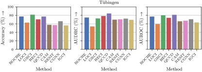
Figure 5: Performance on Tübingen cause-effect pairs datasets. Higher accuracy, AUDRC, and AUROC are preferable. Our ROCHE approach is compared with methods for heteroscedastic noise models: LOCI [9], GRCI [26], HECI [30], and QCCD [27], and methods not designed for heteroscedasticity: CAM [1], RESIT [20], CGNN [4], and ICGI [10]. ROCHE provides promising results and performs significantly better than LOCI with Gaussian likelihood estimation. In general, methods with heteroscedasticity have better performance compared to methods that do not assume heteroscedastic noise models.

5.2 Performance on Synthetic Additive, Location-Scale, and Multiplicative Noise Datasets

Figure 2 illustrates the results of all considered approaches on the AN, AN-s, LS, LS-s, and MN-U datasets. Our ROCHE approach achieves the perfect results in all of these datasets which demonstrate our model’s ability to estimate effectively synthesized heteroscedastic noise data, and special cases including homoscedastic/additive noise and multiplicative noise data. LOCI, which uses neural networks with Gaussian likelihood estimation, has some misspecified cases in LS and LS-s datasets. One case where the causal direction is wrongly predicted has already been presented in Figure 1. The reason for these misspecified pairs is due to the suboptimal fit of the variance in regions with low sample densities. Other methods designed for heteroscedasticity, which are GRCI, HECI, and QCCD, have some pairs misidentified, especially when the generative functions are invertible on AN-s, LS-s, and MN-U datasets. CAM and RESIT achieve perfect scores on the assumption-satisfied additive noise datasets but as the datasets become more difficult these methods cannot perform stably. With no assumption in the structural model, CGNN performs well on AN and LS datasets. However, this approach is also affected by invertible generative functions. Despite not being designed for heteroscedastic noise models, IGCI has nearly perfect results in all cases.

5.3 Performance on More Complex Synthetic Datasets

The results for the 7 remaining simulated datasets are presented in Figures 3 and 4. These results show that our approach can adapt better to diverse model configurations and noise distributions compared to other approaches. On SIM, SIM-ln, and SIM-G datasets, our ROCHE’s results are the best ones in the group of methods with heteroscedastic design. On confounding cases in the SIM-c dataset, our method is more robust and retrieve the causal directions more accurately than other current models. In most cases, the Student’s $t$-distribution estimation approach in ROCHE provides better results compared to the Gaussian estimation in LOCI and the conditional mean and condition mean absolute deviation estimation in GRCI. Noticeably, regression-based methods that regress the residuals and use independence testing for determining causal direction, such as ROCHE, LOCI, GRCI, and RESIT, have demonstrated superior performance in the scenario when confounding variables are present in the SIM-c dataset. Despite having an assumption of low noise levels, IGCI has the lowest distinguishing performance on the SIM-ln dataset. Our approach obtains the second highest results on the Multi and Cha datasets and the highest results on the Net dataset. QCCD predicts decently on the Net and SIM-ln datasets. But on other datasets, the results are less stable with nearly random predictions on the Cha dataset. Although HECI has the best scores on the Multi datasets, this method does not perform as well on the remaining datasets. Homoscedastic methods—CAM and RESIT have high variances in the results among different benchmarks with even sub-standard results on the Multi and Cha datasets. CGNN also exhibits high discrepancy between datasets with decent results in most datasets, except for the SIM and SIM-c benchmarks. On this group of complex benchmarks, our approach has the most stable performance across these diverse benchmark datasets.

Table 1: Overall performance on 13 benchmarks. Reported results are the mean$\pm$std of the Accuracy, AUDRC, and AUROC across the benchmarks. Higher Accuracy, AUDRC, and AUROC are preferable. The best results are presented in bold style. Our ROCHE approach achieves the best overall results with high stability, which demonstrates the robustness of our method.

Method	Accuracy (%) $\uparrow$	AUDRC (%) $\uparrow$	AUROC (%) $\uparrow$
ROCHE (Ours)	$\mathbf{87.69\pm 10.23}$	$\mathbf{92.86\pm\phantom{0}8.16}$	$\mathbf{92.02\pm\phantom{0}7.90}$
LOCI [9]	$84.24\pm 11.43$	$89.04\pm 13.42$	$88.58\pm 11.66$
GRCI [26]	$83.20\pm\phantom{0}9.44$	$89.73\pm 10.19$	$88.86\pm\phantom{0}8.70$
HECI [30]	$65.25\pm 18.17$	$73.34\pm 21.19$	$69.60\pm 20.97$
QCCD [27]	$78.21\pm 16.61$	$85.77\pm 13.70$	$82.69\pm 15.79$
CAM [1]	$72.42\pm 21.23$	$73.89\pm 21.97$	$72.77\pm 22.33$
RESIT [20]	$64.45\pm 30.48$	$68.36\pm 30.05$	$67.08\pm 29.96$
CGNN [4]	$73.89\pm 15.43$	$83.35\pm 14.48$	$79.87\pm 15.55$
IGCI [10]	$73.69\pm 22.98$	$77.26\pm 24.04$	$76.00\pm 23.54$

5.4 Performance on Real-World Data

In addition to synthetic datasets, we also evaluate our method on the real-world Tübingen cause-effect pairs dataset. The accuracy, AUDRC, and AUROC results on this benchmark are depicted in Figure 5. Utilizing the more robust $t$-distribution for the likelihood in ROCHE instead of the Gaussian distribution in LOCI contributes to a huge performance gain on the Tübingen benchmark. Our approach accomplishes promising results with the second highest in accuracy and the third highest in other evaluation metrics on this dataset which are satisfactory and comparable to other methods. The lower robustness of the Gaussian likelihood estimation on real data affects the performance of LOCI substantially and leads to the method’s lowest AUDRC and AUROC in this benchmark. On the more complicated Tübingen dataset, methods targeted heteroscedastic noise models provide better predictions compared to non-heteroscedastic baselines, especially in the case of CAM and RESIT.

5.5 Overall Performance across All Benchmarks

We summarize the overall performance across 13 benchmarks in Table 1 to have a complete evaluation for all methods. In general, our method has the best average results in all three evaluation metrics with the percentage values of accuracy, AUDRC, and AUROC being $87.69\%$, $92.86\%$, and $92.02\%$ respectively. In addition, ROCHE is more robust in comparison with remaining methods with margins of errors less than $10\%$ in AUDRC and AUROC criteria. The standard deviations of our approach have the second lowest value of $10.23\%$ for the accuracy score, which is slightly higher than the best value of $9.44\%$ from GRCI, and the lowest values of $8.16\%$ and $7.90\%$ for AUDRC and AUROC scores respectively.

6 Conclusion

In this work, we have presented ROCHE, a robust estimation approach for bivariate causal discovery with heteroscedastic noise models. Instead of relying on the Gaussian distribution, as done in previous approaches which may not accurately capture the model parameters, we adopt the more robust Student’s $t$-distribution. This choice allows us to account for sampling variability and extreme values more effectively. We propose a framework for modeling the parameters using the $t$-distribution along with necessary constraints to ensure the resulting estimators are suitable for subsequent cause-effect inference tasks. The effectiveness of ROCHE has been demonstrated through comprehensive experiments, yielding promising results and showcasing the best overall performance across 13 benchmark datasets. Furthermore, our approach exhibits robustness, as evidenced by the lowest overall margins of errors across various evaluation metrics. In future work, we aim to extend our approach to handle multivariate heteroscedastic noise models, thus enhancing its applicability to real-world data scenarios.

References

- [1] P. Bühlmann, J. Peters, and J. Ernest, CAM: Causal additive models, high-dimensional order search and penalized regression, The Annals of Statistics, (2014), pp. 2526–2556.
- [2] N. S. Detlefson, M. Jørgensen, and S. Hauberg, Reliable training and estimation of variance networks, in Advances in Neural Information Processing Systems, vol. 32, 2019.
- [3] B. Duong and T. Nguyen, Bivariate causal discovery via conditional divergence, in Proceedings of the Conference on Causal Learning and Reasoning, 2022, pp. 236–252.
- [4] O. Goudet, D. Kalainathan, P. Caillou, I. Guyon, D. Lopez-Paz, and M. Sebag, Learning functional causal models with generative neural networks, Explainable and Interpretable Models in Computer Vision and Machine Learning, (2018), p. 39.
- [5] A. Gretton, O. Bousquet, A. Smola, and B. Schölkopf, Measuring statistical dependence with Hilbert-Schmidt norms, in Proceedings of the International Conference on Algorithmic Learning Theory, 2005, pp. 63–77.
- [6] I. Guyon, A. Statnikov, and B. B. Batu, Cause effect pairs in machine learning, Springer, 2019.
- [7] P. Hoyer, D. Janzing, J. M. Mooij, J. Peters, and B. Schölkopf, Nonlinear causal discovery with additive noise models, in Advances in Neural Information Processing Systems, vol. 21, 2008.
- [8] C.-W. Huang, D. Krueger, A. Lacoste, and A. Courville, Neural autoregressive flows, in Proceedings of the International Conference on Machine Learning, 2018, pp. 2078–2087.
- [9] A. Immer, C. Schultheiss, J. E. Vogt, B. Schölkopf, P. Bühlmann, and A. Marx, On the identifiability and estimation of causal location-scale noise models, in Proceedings of the International Conference on Machine Learning, 2023.
- [10] D. Janzing, J. Mooij, K. Zhang, J. Lemeire, J. Zscheischler, P. Daniušis, B. Steudel, and B. Schölkopf, Information-geometric approach to inferring causal directions, Artificial Intelligence, 182 (2012), pp. 1–31.
- [11] D. Janzing and B. Schölkopf, Causal inference using the algorithmic Markov condition, IEEE Transactions on Information Theory, 56 (2010), pp. 5168–5194.
- [12] I. Khemakhem, R. Monti, R. Leech, and A. Hyvarinen, Causal autoregressive flows, in Proceedings of the International Conference on Artificial Intelligence and Statistics, 2021, pp. 3520–3528.
- [13] A. N. Kolmogorov, Three approaches to the quantitative definition of complexity, Problems in Information Transmission, 1 (1965), pp. 3–11.
- [14] S. Kpotufe, E. Sgouritsa, D. Janzing, and B. Schölkopf, Consistency of causal inference under the additive noise model, in Proceedings of the International Conference on Machine Learning, 2014, pp. 478–486.
- [15] A. Marx and J. Vreeken, Telling cause from effect using MDL-based local and global regression, in Proceedings of the IEEE International Conference on Data Mining, 2017, pp. 307–316.
- [16] J. M. Mooij, J. Peters, D. Janzing, J. Zscheischler, and B. Schölkopf, Distinguishing cause from effect using observational data: methods and benchmarks, The Journal of Machine Learning Research, 17 (2016), pp. 1103–1204.
- [17] J. Pearl, Causality, Cambridge University Press, 2009.
- [18] J. Peters and P. Bühlmann, Identifiability of Gaussian structural equation models with equal error variances, Biometrika, 101 (2014), pp. 219–228.
- [19] J. Peters, J. M. Mooij, D. Janzing, and B. Schölkopf, Identifiability of causal graphs using functional models, in Proceedings of the Conference on Uncertainty in Artificial Intelligence, 2011, pp. 589–598.
- [20] , Causal discovery with continuous additive noise models, The Journal of Machine Learning Research, 15 (2014), pp. 2009–2053.
- [21] C. Schultheiss and P. Bühlmann, On the pitfalls of Gaussian likelihood scoring for causal discovery, Journal of Causal Inference, 11 (2023), p. 20220068.
- [22] M. Seitzer, A. Tavakoli, D. Antic, and G. Martius, On the pitfalls of heteroscedastic uncertainty estimation with probabilistic neural networks, in Proceedings of the International Conference on Learning Representations, 2022.
- [23] A. Shah, A. Wilson, and Z. Ghahramani, Student-t processes as alternatives to Gaussian processes, in Proceedings of the International Conference on Artificial Intelligence and Statistics, 2014, pp. 877–885.
- [24] S. Shimizu, P. O. Hoyer, A. Hyvärinen, A. Kerminen, and M. Jordan, A linear non-Gaussian acyclic model for causal discovery., Journal of Machine Learning Research, 7 (2006).
- [25] A. Stirn, H. Wessels, M. Schertzer, L. Pereira, N. Sanjana, and D. Knowles, Faithful heteroscedastic regression with neural networks, in Proceedings of the International Conference on Artificial Intelligence and Statistics, 2023, pp. 5593–5613.
- [26] E. V. Strobl and T. A. Lasko, Identifying patient-specific root causes with the heteroscedastic noise model, arXiv preprint arXiv:2205.13085, (2022).
- [27] N. Tagasovska, V. Chavez-Demoulin, and T. Vatter, Distinguishing cause from effect using quantiles: Bivariate quantile causal discovery, in Proceedings of the International Conference on Machine Learning, 2020, pp. 9311–9323.
- [28] H. Takahashi, T. Iwata, Y. Yamanaka, M. Yamada, and S. Yagi, Student-t variational autoencoder for robust density estimation, in Proceedings of the International Joint Conference on Artificial Intelligence, 2018, pp. 2696–2702.
- [29] Q. Tang, L. Niu, Y. Wang, T. Dai, W. An, J. Cai, and S.-T. Xia, Student-t process regression with Student-t likelihood, in Proceedings of the International Joint Conference on Artificial Intelligence, 2017, pp. 2822–2828.
- [30] S. Xu, O. A. Mian, A. Marx, and J. Vreeken, Inferring cause and effect in the presence of heteroscedastic noise, in Proceedings of the International Conference on Machine Learning, 2022, pp. 24615–24630.
- [31] K. Zhang and A. Hyvärinen, On the identifiability of the post-nonlinear causal model, in Proceedings of the Conference on Uncertainty in Artificial Intelligence, 2009, pp. 647–655.
- [32] K. Zhang, Z. Wang, J. Zhang, and B. Schölkopf, On estimation of functional causal models: general results and application to the post-nonlinear causal model, ACM Transactions on Intelligent Systems and Technology, 7 (2015), pp. 1–22.