./resources/svg/Thesis/resources/svg/

ESTIMATION OF PHYSICAL PARAMETERS OF WAVEFORMS WITH NEURAL NETWORKS

Master Thesis

For obtaining the degree

Master of Science (MSc)

at the Faculty of Natural Sciences

Paris Lodron Universität Salzburg

&

Faculté Sciences & Sciences de l’Ingénieur, Université Bretagne Sud


Submitted by

Saad Ahmed Jamal

Dr. Thomas Corpetti

Université Bretagne Sud, France

Prof. Dr. Dirk Tiede

Paris-Lodron-Universität Salzburg, Austria

Ms. Mathilde Letard

Université de Rennes 1, France

Dr. Dimitri Lague

Université de Rennes 1, France

June 2023

List of Acronyms

LiDAR

Light Detection and Ranging

MAE

Mean Absolute Error

RMSE

Root Mean Square Error

GIS

Geographical Information System

UAV

Unmanned Aerial Vehicle

WALID

A new LiDAR simulator for Waters

ANN

Artificial Neural Network

CNN

Convolutional Neural Network

RNN

Residual Neural Network

LUT

Look Up Table

DTM

Digital Terrain Model

TIN

Triangluar Integrated Network

FWL

Full Waveform LiDAR

GPU

Graphical Processing Unit

GB

Giga Bytes

ResNets

Residual Networks

RF

Random Forest

SVM

Support Vector Machine

kd

Attenuation coefficient

Funding

This research was supported by European Union, Erasmus Mundus Joint Master scholarship program, Copernicus Digital Earth (https://www.master-cde.eu/).

Abstract

Light Detection and Ranging (LiDAR) are fast emerging sensors in the field of Earth Observation. It is a remote sensing technology that utilizes laser beams to measure distances and create detailed three-dimensional representations of objects and environments. The potential of Full Waveform LiDAR is much greater than just height estimation and 3D reconstruction only. Overall shape of signal provides important information about properties of water body. However, the shape of FWL is unexplored as most LiDAR software work on point cloud by utilizing the maximum value within the waveform. Existing techniques in the field of LiDAR data analysis include depth estimation through inverse modeling and regression of logarithmic intensity and depth for approximating the attenuation coefficient. However, these methods suffer from limitations in accuracy. Depth estimation through inverse modeling provides only approximate values and does not account for variations in surface properties, while the regression approach for the attenuation coefficient is only able to generalize a value through several data points which lacks precision and may lead to significant errors in estimation. Additionally, there is currently no established modeling method available for predicting bottom reflectance. This research proposed a novel solution based on neural networks for parameter estimation in LIDAR data analysis. By leveraging the power of neural networks, the proposed solution successfully learned the inversion model, was able to do prediction of parameters such as depth, attenuation coefficient, and bottom reflectance. Performance of model was validated by testing it on real LiDAR data. In future, more data availability would enable more accuracy and reliability of such models.

1   Introduction

1.1   Background

Light Detection and Ranging (LiDAR) is an active remote sensing technology that is used for high-resolution mapping. It makes use of laser beams to provide spatial data of high resolution. Modern sensors have resolution of few centimeters.

A typical LiDAR instrument consists of a laser, a scanner, and a specialized GPS receiver. The principle of LiDAR is to measure the time of flight taken by the pulse to reach the receiver from the transmitter after reflecting from the object. The analysis of the back-scattered signal (in particular its maxima), also called waveform, enables to derive 3D point clouds related to encountered objects (EP. Baltsavias, 1999; Mallet  Bretar, 2009; Mehendale  Neoge, 2020). It is to be noted that LiDAR can only measure distance using time measurements.

$$D=c(\Delta t/2)$$ (1)

where, D is the distance of the object, c is the speed of light and $\Delta$t is the time required to travel by the laser. LIDAR scanning mechanism is mainly classified into four types (i) Opto-mechanical (ii) electro-mechanical (iii) micro-electro-mechanical systems (MEMS) (IV) solid-state based The electro-mechanical scanning is mostly used in LIDAR nowadays (Raj ., 2020). Efforts are been made to Solid State Scanning to use it more often due to its potential robustness, field of view (FOV), and scanning rate potential. The resolution or minimum detectable object essentially depends on the reflectivity of the object. There are several other factors such as atmospheric conditions, irradiation of background, type of target, level of noise, laser wavelength, aperture, detector sensitivity, angle of inclination of surface, and shape of target E. Baltsavias (1999). contributing to detectability.

Waveform and point cloud are two types of data that can be obtained from Lidar. Waveforms are time series of the complete back-scattered signal, while point clouds are obtained through the processing of the waveforms. In the waveform, each major peak corresponds to an object encountered by the laser beam (Letard, Collin, Lague ., 2022).

Topo-bathymetric Lidars use a green laser in addition to the IR one because green lasers are able to reach the ground below the water surface. Topobathymetric Lidar, being an active sensor with the ability to penetrate the water surface, can gather data from both the water surface and the ground beneath it near the land water interface regions (Lague  Feldmann, 2020).

Uses of LIDAR in remote sensing include terrain mapping, digital elevation modeling, forest inventory, biomass estimation, coastline and beach mapping, floodplain mapping, river channel mapping, urban planning, building height determination, mining, and mineral exploration, archaeological site mapping, snow mapping, oceanography and coastal zone management, precision agriculture, and crop mapping and transportation infrastructure and asset management (Mallet ., 2009; Mehendale  Neoge, 2020).

The disadvantages of LIDAR include high cost for data acquisition, and maintenance, large data volume, complex data processing, potential gaps, limited footprint, and wavelength range (Beland ., 2019). It is a line-of-sight technology. LIDAR waves are also affected by weather and the object with which it interacts.

1.2   Research Objectives

Following were the objectives that were pursued during the research:

1. create a large amount of simulated data

2. design a deep neural network using simulated data

3. evaluate performance on real data

1.3   Significance

This study is the first attempt to predict parametric values by learning patterns through the LIDAR waveform. The current knowledge domain lacks accuracy to invert and retrieve these parameters. Out of the three parameters under study: depth, attenuation coefficient and bottom reflectance, for bottom reflectance, no current modeling method exist. Depth can be estimated through inverse modeling. The attenuation coefficient can also be approximated to some extent through regression of logarithmic intensity and depth. Nevertheless, these approximations lack a significant degree of accuracy. This research proposed to learn the inversion model with the help of neural networks. Also, this approach requires less computational power as compared to solving inverse problems. This will provide a new dimension for LIDAR data analysis, and increase productivity and usefulness.

1.4   Motivation

LiDAR are rapidly becoming popular for ground mapping. They have proved their reliability for various applications in oceanography, forestry, hazard monitoring and geology. Geographical Information System (GIS) world have been knowing about the sensor for a decade but other systems are now adopting it for multiple uses. For example, LiDAR are now being used in smartphone for better quality of photography. New generation Iphone 13 Pro contains LiDAR sensor which provides 3D animations. Modern sensors are allowing high resolution mapping on large scale. Topo-Bathymetric LiDAR are replacing previous means of seismic and bathymetric surveys near the ocean water and land interface which were extremely expensive and cumbersome. Unmanned Aerial Vehicle (UAV) equiped with LiDAR allows repetitive surveys which is now being used for temporal analysis. This study would further enhance usage of LiDAR data by extracting more important information, making it more interesting for different bathymetric applications and research, assisting Copernicus services for Marine and Security.

1.5   Organization of Thesis

The rest of the thesis is organized as follows. Section 2 describes literature related to the topic. Section 3 describes the methods and the experimental setup. Section 4 illustrates the results and discussion of the experiments, provides insight for future research, and Section 5 concludes the study. The later part includes: bibliography and appendixes.

2   Literature Review

WALID is a simulator that produces waveforms for flooded (water-covered) areas similar to one coming from an actual LIDAR sensor (Abdallah ., 2012). LASER wavelength, generated by the simulator, is from 0.3 to 1.5 micrometers which corresponds to the ultraviolet to infrared range. GLAS/ICE-SAT is a satellite that provides altimeter data through elevation measurements (Baghdadi ., 2011). For the infrared region, GLAS system characteristics were used for the simulation of waveform while for the visible range in A new LiDAR simulator for Waters (WALID). HawkEye LiDAR is an airborne sensor for bathymetry (Chust ., 2010). It can measure sea bottom elevation in low water depth areas. GLAS and Hawkeye were used for comparison of the observed waveform from the simulated waveform using signal-to-noise ratio and homothetic transformation. The novelty of the WALID simulator model lies in that it takes into account the physical properties of water, such as the transfer of energy in the form of electromagnetic radiations through a medium (laws of radiative transfer). There are several other such simulators available. Virtual environments such as computer games were used as simulators. GTA-V game was used to generate a large amount of realistic training data in a virtual environment (Wu ., 2018). Squeezeseg, a network based on the convolutional neural network was used for semantic segmentation and point-wise classification of the simulated data.

LidarNet developed by Aßmann . (2021) regenerates the waveform datasets for any specific parameters. According to their statement, they have achieved a 99% accuracy by employing a model based on Convolutional Neural Network (CNN). The authors trained a classifier on simulated data and achieved favorable results for validation on unseen real data.

Andersen . (2005) created a regression model for forest canopy fuel estimation. For all parameters, a strong correlation was discovered between metrics derived from LIDAR data and fuel estimates obtained through field-based measurements. The research showed that LIDAR-based fuel prediction models can be used to develop maps of canopy fuel parameters over forest areas. Koetz . (2006) used LIDAR waveform for estimation of biophysical parameters of the forest. The forest canopy structure was determined by deriving parameters such as leaf area index, vertical crown extension, maximum tree height, and fractional cover. Two sets of data, synthetic and real, were used to evaluate the accuracy of the new method. The data included laser waveforms and associated forest canopy information, which was used to assess the performance of the proposed approach. A synthetic data set was created by simulating the waveform response of 100 simulated forest areas using the LIDAR waveform model described earlier. A real-world dataset was collected in the Eastern Overpass Valley, an area located within the Swiss National Park. The process of extracting information from the LIDAR waveform model was based on a Look Up Table (LUT) method. This approach involves two steps: building the LUT itself and selecting the appropriate solution that matches a specific measurement. The result of the model inversion was determined by reducing the value of the merit function $(X^{2})$, which measures the difference between the reference waveform $(w_{ref})$ obtained from the laser system and the simulated waveform $(w_{sim})$ stored in the LUT. The simulated waveforms were scaled based on their highest peak, making them consistent with the recorded signal.

$$X^{2}=\sum\limits_{i=1}^{n_{bin}}\,(w_{ref}^{i}-w_{sim}^{i})$$ (2)

Our research proposed the estimation of physical parameters of LIDAR waveform using deep neural networks which is also a type of inverse problem. It is also common to use observations of the physical system to solve the inverse problem, that is, to learn about the values of parameters within the model, a process that is often called calibration. The main goal of calibration is usually to improve the predictive performance of the simulator (Brynjarsdóttir  O’Hagan, 2014).

Mallet . (2009) reconstructed the waveform through a set of parametric or modeling functions. LIDAR data is used to generate Digital Terrain Model (DTM) that is used in many physical studies such as river flow modeling. Mandlburger . (2009) presented a DTM thinning approach for the effective use of LIDAR data for the generation of Triangluar Integrated Network (TIN). It is used as input for predicting the behavior of complex physical systems. Deep Convolutional Neural Networks were used for building extraction using LiDAR data (Maltezos ., 2019). Chen . (2022) used them for power transmission line detection.

To effectively utilize observations of a physical system, it is essential to acknowledge the concept of a model discrepancy, which refers to the difference or mismatch between what the simulator predicts and what actually occurs in reality. This recognition is crucial as it allows us to identify and address any inaccuracies or limitations in the model, leading to more reliable and accurate predictions of the real-world system. Analysis that does not account for the model discrepancy may lead to biased and over-confident parameter estimates and predictions. In statistical inverse problems, accounting for model discrepancy can be challenging because it can be difficult to distinguish the effects of model discrepancy from the effects of calibration parameters (Brynjarsdóttir  O’Hagan, 2014). To properly address this challenge, it is necessary to incorporate meaningful priors on the model parameters that reflect our knowledge or beliefs about the true values of those parameters. Only then can we accurately separate the effects of model discrepancy and calibration parameters and make accurate inferences about the true system.

Full waveform (FW) is state-of-the-art LiDAR technology (Mallet  Bretar, 2009). It offers more control in the interpretation of measurements by end users, as it provides detailed information about the structure and physical back scattering of the illuminated surfaces. This supplementary information can be used to better understand the domain and can assist in the interpretation and analysis. Pulsed or Discrete systems measure the round-trip time while continuous wave systems carry out ranging by measuring the phase difference between the transmitted and received signal. Full Waveform LiDAR (FWL), for each pulse, is able to record almost the entire back-scattered signal (Liu  Ke, 2019). Due to this reason, typically the size of FW data is 10 times larger. The processing also is not easy as fewer packages exist for its visualization and processing.

Artificial Neural Network (ANN) have been used for the estimation of physical and abstract parameters. ANN was used by Calderón-Macías . (2000) for geophysical parameter estimation such as formation resistivity and layer thickness. Seismic waveform data was used as input data for the feed-forward neural network. Such deep learning frameworks have proven to be useful for the analysis of LIDAR data. Algorithms act as a set of mathematical transformations (Maltezos ., 2019; M. Nusrat ., 2023). For problems such as building detection, mathematical computations alone are not adequate to model the physical properties of a problem, In such cases, raw LIDAR data has to be augmented with features coming from the physical interpretation of data.

LIDAR Data had been used for tasks beyond height extraction. Guiotte . (2020) used it for semantic segmentation. Though the sparse nature of point clouds makes them inappropriate for many image analysis tools, therefore it is rasterized to avoid this problem. Frequently, it is rasterized as Digital Elevation Model (DEM) (Jamal  Aribisala, 2023). It is used for future precipitation impact studies and river flow modeling using learning-based approaches (A. Nusrat ., 2020, 2022). Green LIDAR waveform complemented by infrared point cloud had been used for classification of land-water habitat with accuracy up to 90 (Letard, Collin, Corpetti ., 2022). The full waveform was used for seagrass mapping (Letard, Collin, Lague ., 2021). Using bispectral full waveform LIDAR, coastal habitat can be mapped seamlessly with accuracy up to 97 percent (Letard, Collin, Lague ., 2022). Data fusion of full waveform LIDAR with hyperspectral imagery was used for tree species classification using auto-encoder (Liao ., 2018). Heinzel  Koch (2011) achieved an accuracy of 57% within six species of trees while 80% was achieved for classification among 4 main species.

Solely on the basis of FWL, 92% accuracy was achieved by Zorzi . (2019) for classification within 6 different land cover classes. The classes were ground, vegetation, building, power line, tower, and street. The researchers introduced a new architecture exploiting both full waveform and spatial information. The network is able to classify full waveform directly without the need for prior extraction of features. Thus, it can be applied to FW data for any area. The network includes two CNNs. First CNN is responsible for the conversion of FW data into images. The second part is a UNET model that is used for the segmentation of images. The output of the first part is fed as input to the second. In this way, the resultant output shows better overall and per-class accuracy. The latest research by Marinelli . (2022) resulted in a further increase in overall accuracy.

LIDAR is being used in snow hydrology and avalanche sciences applications for snow depth mapping. It has numerous advantages over manual surveys and other sensors with larger footprints as demonstrated by Deems . (2013).

Morphological features can be fetched from waveforms. Mallet . (2011) classified urban area points into buildings, ground, and vegetation points. Two FW processing methods were used which are the marked point process approach and the non-linear least squares method. The higher average accuracy of the classification was achieved using full-waveform data than discrete return data.

Convolutional Neural Network (CNN) has been the most effective deep learning approach for dealing with image data. Temporal Convolutional Neural Network developed by Pelletier . (2019) introduces an effective deep learning approach for classification time series data. This technique utilizes temporal convolutions (convolutions in the temporal domain) to automatically learn both temporal and spectral features. This led to better results than Random Forest (RF) and Recurrent Neural Network (RNN) with a margin of about 1-3% in overall accuracy. However, the lack of integration of spatial domain causes salt and pepper noise in the results. Three convolutional layers with 64 units, one dense layer with 256 units, and one softmax layer make up the architecture. The paper also demonstrates the effect of filter size, batch size, depth of model, pooling, and spectral and temporal dimensional guidance. Hybrid methods have proven to be more effective when dealing with time series data. Hybrid methods combine quantitative time series models together with deep learning

Several techniques are in use for bathymetric mapping. Spectral methods can measure depths up to 2 to 2.5m with a mean error of the order of 15–20cm. Structure From Motion which is using stereo imaging for 3D modeling is also used to measure heights. However, it is not effective for measuring through water as it is effective only up to 2m inside water. Coastal bathymetric with airborne LIDAR uses green laser 532nm which is one of the least absorbed wavelengths. It is able to measure depths up to 40–50m. However, the cost of such a survey is higher than 1000€/km². Multibeam Sonar is the most useful method for measuring deep water courses. With a range of up to 100 to 4000m, it makes use of sound waves to propagate through the water to produce a bathymetric map (Fairfield  Wettergreen, 2008). The limitation of this technique includes lesser efficiency for bathymetry at shallow water depth.

Topo-bathymetric through airborne LIDAR though is not capable of going hundreds of meters into the water, yet it is a useful technique for high-resolution and high-precision surveys. Awadallah . (2023) did a comparison among different bathymetric sensors. They concluded that these sensors are able to provide high-quality river geometry representation. It can penetrate up to 80m into water. The penetration depth depends on several factors such as the wavelength of the laser, the power of the system, the reflectivity of the seafloor, and the water quality such as turbidity, viscosity, surface roughness, and suspended particles in water. Many of the physical parameters of water are unknown which makes it difficult to calculate the empirical penetration depth (Lague  Feldmann, 2020).

The backscatter signals over water for full waveform consist of three parts. 1) Surface echo when the wave strikes the surface, 2) an exponential attenuation of the signal in the water column because of absorption by water and suspended particles, and 3) bottom echo that corresponds to bed reflectivity. Depending on bottom topography, the shape of the backscattering echo differs (Szafarczyk  Toś, 2023). Topo-bathymetric LIDAR has the potential to replace numerical models based on channel cross-sections that are used for large-scale hydraulic modeling. A similar network was used by (Letard, Collin, Corpetti ., 2021) for the classification of coastal and estuarine ecosystems.

Awadallah . (2023) analyzed the discrepancies in altitude among the bathymetric, MBES, and TLS point clouds. It also assessed the differences in altitude within the bathymetric LiDAR point clouds and connected these variations to river characteristics such as depth, bank inclination, sudden changes in altitude, and turbulent areas. The bathymetric measurements acquired in the Autumn season tend to have more errors with lesser penetration within water than the ones acquired in winter (Islam ., 2022). This seasonality effect is due to higher sediment concentration in Autumn.

Attenuation is the reduction in the strength of a signal, wave, or other form of energy as it travels through a medium. Attenuation can occur due to various factors such as absorption, scattering, reflection, and dispersion. Based on the backscattering of the LiDAR beam, equation 3 was developed by Yang . (2022) for calculating the attenuation coefficient of water. The attenuation coefficient was measured as 1.343 for their experiments.

$$\ln(E_{i})=-C(z+0.2)+\ln(\eta E_{0})$$ (3)

where C is the attenuation coefficient of water, E0 and Ei is the sent and received power of source light, and z is the measuring distance between the reflector and light source.

3   Methodology

The aim was to determine the parameters of the target water body from waveform mainly reference depth of water, attenuation coefficient for the water, and bottom reflectance. In this research, primarily, we made use of a simulator called Walid (Abdallah ., 2012) to generate a large amount of sample waveforms. The simulator was accessed through an anaconda interface. Simulated data was generated for interaction of LiDAR signal over water body for the purpose of bathymetry. This was set by defining a set of input parameters which are described later in table 1. The simulated data was meant to be fed to the neural network for making the prediction of the required parameters. The reason for using simulated data was in order to train a deep neural network, one needs to have a large amount of input data. LiDAR surveys are expensive. Real data is not readily available and is costly. So it was not possible to gather an ample amount of real LiDAR data to train an efficient neural network. The strategy chosen was to train the network on simulated data and use the real LiDAR data for validation purposes. Also, In general, the larger the amount of data, the better weights are learned and the better the neural network. So, the option to train using simulated data seemed to be effective as an ample amount of simulated data could be generated using GPUs.

A common question often addressed during the research was why to use deep learning instead of inverse models or mathematical models or any other? It is because, for these parameters, there exists no such model except for one parameter which is depth. Depth can be calculated using inverse modeling but that too is computationally expensive. So deep learning is more useful in such cases. Scalability is one of the main advantages of deep learning models that they show good performance with large amounts of data. The deep network was coded using the TensorFlow library in Python. Figure 1 presents an abstraction of methodological flowchart.

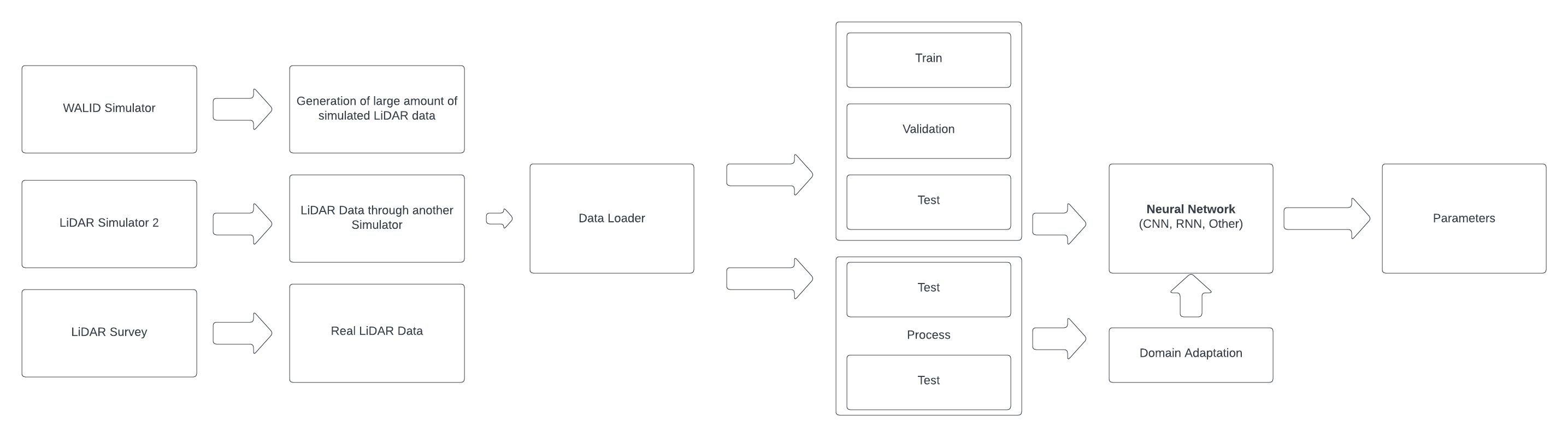
Figure 1: Methodological Flowchart

The network first was trained to learn and approximate the relation between the optical parameters and backscattering of signal from the water, which will result in a data-driven model capable of mapping the relationships among the parameters and waveform. The second task is to invert this model to solve the inverse problem so as to produce parameters that will honor the known waveform and reproduce the water characteristics. This paper explains the Neural Network training and the inversion process and demonstrates that the process works using a hypothetical problem where the input and outputs are assumed and therefore the performance of the inversion process can be quantified. Consequently, simulated cases allow for a better evaluation of the accuracy of the technique used to estimate the missing parameters.

The total power received by LIDAR is the sum of these parameters with the addition of factors.

$$P_{T}(t)=P_{s}(t)+P_{c}(t)+P_{b}(t)+P_{bg}(t)+P_{n}(t)$$ (4)

where $P_{T}(t)$ is the total power received, $P_{s}(t)$ is the power returned by the water surface, $P_{c}(t)$ is the power returned by the water column, $P_{b}(t)$ is the power returned by the bottom, $P_{bg}(t)$ is the background power returned by the air column, Pn (t) is the detector noise power and t is the time scale. A time series is a collection of data points measured at regular intervals over time.

3.1   Generating Large amount of Data

First, it was essential to produce a large amount of training data. WALID simulator was used with suitable parameters to generate many datasets.

Parameters were to be selected according to the Titan sensor so to simulate a waveform similar to the real LiDAR sensor, recorded by the sensor for the green wavelength. The parameters were Amplitude (scales the whole waveform), Imp_type (extreme dist, GevII), a sampling interval of data, the base intensity of waveform, noise, and reference intensity of water surface echo. Apart from these, medium parameters were also selected such as reference intensity of water decay (I_w), the attenuation coefficient of water (Kd), bottom reflectance (I_ref), depth of water, and maximum depth of the medium.

Generating large amounts of data was not possible local desktop computer. A cluster provided by UBS was used for the task. The cluster which can be referred to as a high-performance computing facility was a group of computational resources that was made available for research purposes. IRISA’s (Institut de Recherche en Informatique et Systèmes Aléatoires) cluster had mainly Graphical Processing Unit (GPU) resources as research had leaned towards Deep Learning. with support of up to 1152 Giga Bytes (GB) of Graphical Memory with individual GPU units of 256 GB. The cluster was accessed through a Linux interface in the Ubuntu operating system. Two types of job posts could be posted. Short Run: if the job is less than 48 hours, Long Run: if the job is estimated to run for more than it.

Waveform generator code was uploaded onto the cluster after making subtle changes. 1 Million waveforms were generated using the cluster. It took 14.2 hours to simulate 1 Million training samples. With this large number of training data, it was possible to train the neural network to a better model. Figure 2 shows a few samples of simulated waveforms where the y-axis shows the intensity of the received signal.

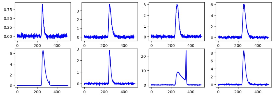
Figure 2: Simulated Waveforms

3.2   Study Area

Frehel is a picturesque coastal commune located in the western region of France called Bretagne. Situated along the Emerald Coast along the English Channel, Frehel offers breathtaking natural beauty. With its stunning cliffs, sandy beaches, rugged landscapes, and a low number of inhabitants. The study area is located from geographic coordinates. Figure 3 shows satellite view of study area.

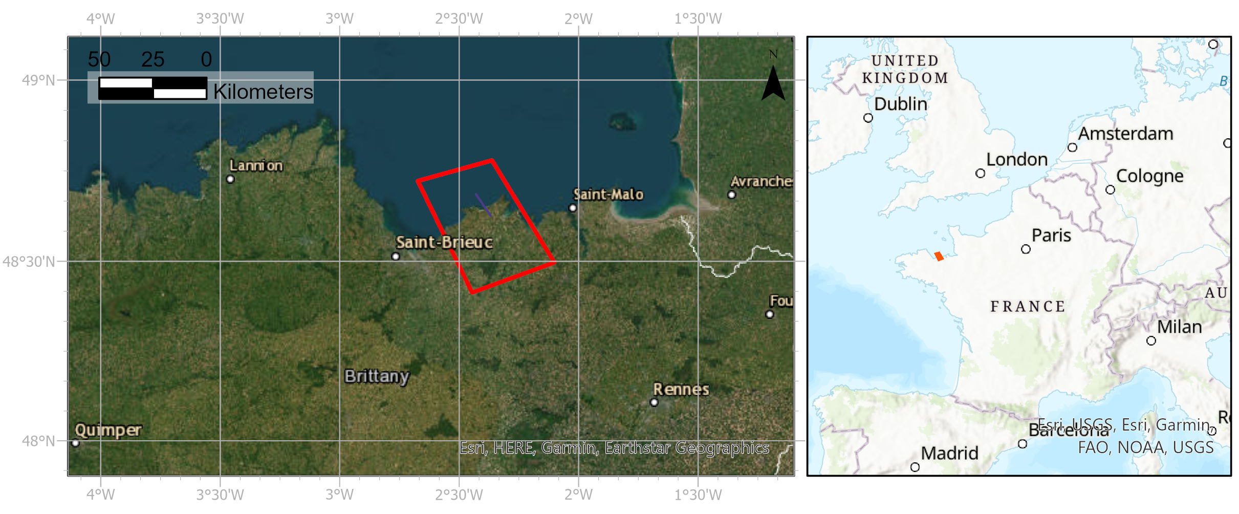
Figure 3: Study Area Map

3.3   Sensitivity Analysis

An analysis was performed for deriving the effect of different parameters model to check their effect on the model performance. These parameters include batch size, train-validation split ratio, choice of the optimizer, and learning rate. Also, other factors were examined such as the effect of noise on data, activation functions, kernel size, number of trainable parameters, feature maps, and convolutions depth.

3.4   Design of Model

Then came the design of the most appropriate model that minimizes the loss and error in the prediction of parameters. When working with one-dimensional data as input, learning-based models have proved to be useful. Residual Neural Network (RNN), Convolutional Neural Networks (CNN), Transformer Based Networks, Autoencoders, and Generative Adversarial Networks (GANs) are best suited for the task. Machine Learning (ML) algorithms such as Support Vector Machine and Random Forest Regressor were also evaluated which previously were quite efficient for supervised learning tasks. With the bloom of deep learning, after AlexNet in 2012, they tend to outperform the machine learning models which proved to be the case in these experiments as well. It is due to several reasons like their ability to automatically learn hierarchical representations of data. This means that they can extract meaningful features or representations directly from the raw data without the need for manual feature engineering. This automation is often referred to as end-to-end learning. They capture intricate patterns and generalize well, especially in scenarios where large datasets are available. Layers with non-linear activation functions, allow modeling of complex patterns and dependencies. ML models, such as linear regression or decision trees, perhaps, struggle to represent such non-linear relationships. The choice of modeling approach depends on the specific problem, the available data, the computational resources, and other factors. Different types of models and approaches may be more appropriate in certain scenarios, and it’s crucial to consider the trade-offs and requirements of the problem at hand. Therefore, ML models were also tested to check their usability in this case.

To have the best model, different types of RNNs, CNNs, and Autoencoders were experimented with. GANs are not useful for dealing with waveforms because they are more focused on stable diffusion tasks.

The training of neural networks was not so straightforward. It included challenges some of which were unforeseen. Therefore, a more step-wise progressive approach was followed. Initially, a simple CNN was designed to check the learning process. The affect of different factors such as training size, noise in data, and depth of convolutions were tested. The input shape of training batch was set as (12, 512,1) where 12 was the batch size, 512 was number of time stamps, and 1 is the number of bands. Number of bands was set to one since the waveform generated corresponded to green wavelength band of LiDAR signal. Whereas in future if more LiDAR data with more bands would be available, it can be incorporated by changing the number of bands. Hence, adding to the modality of the network. The simulated data was stored in hdf5 format. A dataloader in python was used for loading and spliting the data into train, validation and test set. 80:15:5 ratio was used for the split respectively.

3.5   Convolutional Neural Network

Convolutional Neural Network (CNN) consist of convolutional layers which are the main building block of CNN to automatically learn and extract hierarchical representations of the input data. Each layer consists of one or more filters often referred to as feature maps that are convolved with the input data. Convolution is a mathematical operation that applies a sliding window or filters over the input data, performing element-wise multiplication and summing the results. Convolution helps to detect local patterns and features in the input data. After convolution, usually, it is followed by a pooling layer that is often employed to reduce the spatial dimensionality while preserving the important features. This downsampling of feature maps makes the model more robust to variations and distortions in the input. Common pooling operations include max pooling, which retains the maximum value within each pooling region. Other pooling types include average pooling and min pooling. After pooling, usually comes the activation function. CNN can have linear and nonlinear activation. Non-Linear Activation Function was one of the main breakthroughs in deep learning and resulted in the rebirth of deep learning. One such function is Rectified Linear Unit (Relu). It introduces non-linearities, allowing the model to learn complex relationships and capture non-linear patterns in the data. After the convolutions, towards the end of the network, fully connected layers are employed to integrate the extracted features and make predictions. These layers connect every neuron from the previous layer to every neuron in the current layer. Fully connected layers are typically followed by an activation function and a final output layer that produces the desired floating point or categorical values depending upon the last activation. Typically softmax activation function is used for classification tasks while other activation functions such as relu in-case of regression.

CNNs have achieved significant success in various domains, including image classification, object detection, and image segmentation. They exploit the local correlations, spatial structure, edges, textures, and patterns. This property makes them well-suited for tasks where local details are important. CNNs are particularly effective in these tasks because of their ability to capture local features and patterns, that too with a lower number of trainable parameters compared to conventional deep networks of similar depth, making them more implementable for practical applications (Alzubaidi ., 2021).

A common myth, that some people think that CNNs are limited to image-related tasks is not true as they have been proven to be useful in other domains as well such as one-dimensional and time series data. With waveforms being 1D convolution, 1D convolutional layers were used to build the network. To come up with the best model, it was experimented with varying designs. This includes changing a number of convolutions (convolutional depth), filters, pooling, batch normalization, encoding, decoding, and regularization. The maximum depth that could be attained with pooling after each convolution was nine due to the shape of the input signal. Though with different settings depth was increased further.

3.6   Recurrent Neural Network

Recurrent Neural Networks (RNN) could be highly useful for analyzing and modeling waveforms due to their ability to capture temporal dependencies and sequential information. Their success is in audio analysis, time-series forecasting, and other tasks where understanding the temporal dynamics of the data is crucial. RNNs have feedback connections that allow information to be passed from previous time steps to the current time step. This recurrent connectivity enables RNNs to capture and model sequential dependencies in the data.

There are four types of RNNs that are useful for dealing with sequential data.

• Long-Short Term Memory (LSTM)

• Bidirectional LSTM

• Gated Recurrent Unit (GRU)

• Attention Based Network

RNNs were tested by varying numbers of recurrent layers for each type of network.

3.7   Other Networks

Apart from these, several other networks, that were originally developed for other tasks, including pre-trained and fine-tuned models were tested. These include Resnet 50, 1D soat waveform, Transformers, and Wavenet. Deep learning models are often criticized for their lack of interpretability. By comparing them with other machine learning models, one can determine if interpretability is important for the problem. If interpretability is a priority, one might choose a model that provides more transparent decision-making, such as Support Vector Machine (SVM) or Random Forest (RF). So, the performance of ML models was also compared with the other deep learning models.

Residual Networks (ResNets) are deep CNN architectures that introduce skip connections, allowing for better gradient flow and alleviating the vanishing gradient problem. ResNets are effective in capturing both local and global features in waveform data. By enabling the network to learn residual connections, they can handle deep architectures and extract more complex representations. Transformer models, such as the ones used in natural language processing tasks like machine translation and language modeling, can also be applied to waveform data. The self-attention mechanism in transformers allows them to capture long-range dependencies in the waveform. These models can be used for tasks like speech synthesis, music generation, and audio-to-text conversion. BERT Transformer model was modified and tested for its performance with waveforms. WaveNet is a deep generative model that utilizes dilated convolutions to model and generate waveforms. It has been specifically designed for speech synthesis and has demonstrated excellent performance in generating realistic waveforms. WaveNet can also be adapted for waveform parameter prediction tasks by modifying its output layer

3.8   Domain Adaptation

Domain adaptation was used for adjusting the real LiDAR data in accordance with the simulated data in order to improve the performance of the model. It is sub-field of transfer learning to enhance a model’s performance on a target domain with insufficient annotated data by utilizing the model’s knowledge from a related domain with sufficient labeled data (Farahani ., 2020). It is commonly used technique in remote sensing especially with respect to satellite imagery. The satellite images of different places show different characteristics for example, satellite image from Pakistan will be different from the one in Austria or France. Therefore, for any task such as land use classification, a model that is trained on one might not perform good enough on the other.

Figure 4 shows a plot of normalized waveforms, which demonstrates the need of domain adaptation of the data.

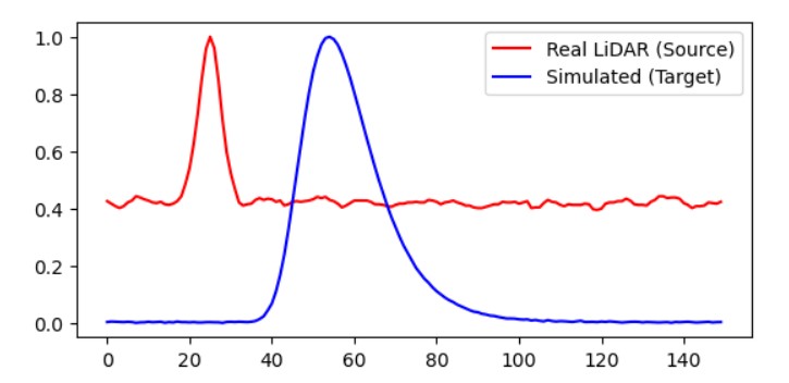
Figure 4: Difference between Waveforms

For validation of our model, the trained model was used to predict labels for another simulated data that was generated using a different simulator. The model could predict the labels but without any further training, the results were not good enough. With a slight amount of training on the other data, the model improved significantly leading to to better predictions. The coefficient of determination, r2 score, jumped up to 0.49.

In order deal with Light Detection and Ranging (LiDAR) dataset that were generated from different simulators, Domain Adaptation techniques were explored. Multiple typed of domain adaptation techniques were tested including data adaptation and model adaptation. For data adaptation, optimal transport was used made by Courty . (2017).

One of the main challenges of domain adaptation is that labeled data may not be available in the target domain. This makes it difficult to train a classifier that can generalize well to new data in that domain. Unsupervised domain adaptation is the one in which labeled data is not available in the target domain. This makes it difficult to train a classifier that can generalize well to new data in that domain. To address this challenge was by finding a common feature representation for both domains which is called latent space. This allows for labeled samples from the source domain to be used to train a classifier that can be applied to the target domain as well. Courty . (2017) proposed a regularized unsupervised optimal transportation model to align these representations and exploit both labeled samples and distributions observed in both domains. Thus deriving a probability density functions (PDFs) of the source and target domains. Among the unsupervised domain adaptation, sinkhorn transport worked better.

3.8.1   Optimal Transport

Optimal Transport is a mathematical function that quantifies the optimal way to redistribute mass or resources from one distribution to another. It provides a principled approach to compare and measure the dissimilarity between probability distributions.

In the context of transportation, optimal transport seeks to find the most efficient way to move mass from a set of source points to a set of target points such to minimize the total cost required for the transportation.

The concept of optimal transport is often represented by a transportation plan, A transportation plan is a matrix that specifies how much mass from each point in the source domain should be transported to each point in the target domain. The process of learning a transportation plan involves minimizing an objective function based on optimal transport, which is regularized to ensure that labeled samples of the same class in the source domain remain in close proximity during the transportation process. Courty . (2017) provided a python package for optimal transport that was for experimenting types of optimal transport. The types that were tested were EMD Transport, Sinkhorn Transport, and Sinkhorn Transport with regularization.

4   Results and Discussion

This section presents a comprehensive analysis of the findings obtained from the conducted study. It aims to provide a detailed examination and interpretation of the data, shedding light on the key outcomes and their implications. The study focused on development of simulated data, design of suitable model and estimation of parameters. In this section, obtained results are described, Furthermore, we delve into potential explanations for observed patterns and variations, considering both anticipated and unexpected outcomes. Through a rigorous analysis and contextualization of the data, this section provides insights into the implications of the study findings, their relevance to the research objectives, and their broader implications in the field.

The first task was to check the effect of input parameters for the simulator. An effort was made to simulate waveforms as similar as the Titan sensor waveforms. This was successful to some extent. The following parameters range was used:

Parameter	Low Limit	High Limit
depth	0.15	19
Bottom (Iref)	1	100
kd	0	1
Iw	0	2
A	1	10
noise	0	(0.04)*A
Imp Type	0	2
Wc	0.1	1

Table 1: Input Parameters for WALID Simulator

4.1   Sensitivity Analysis

It is a systematic approach used to assess the responsiveness of a model or process to variations in input parameters. It involves systematically changing the values of input variables within a defined range and observing the resulting changes in the model’s output or outcomes. The primary goal of sensitivity analysis is to understand how changes in the input parameters impact the output and to identify which inputs have the most significant influence on the model’s results. By conducting a sensitivity analysis, researchers and analysts can gain insights into the robustness, reliability, and stability of a model or system. Thus this step helped in decision making for selection of suitable mode.

4.1.1   Effect of Noise

Adding enough noise in the data made it more closer to the actual data. It improved the model performance by making training process more robust. Such was the case with the experiment. Adding small amount of noise in the data, improved the model performance (Bishop, 1995). Injecting noise in the input to a neural network can also be seen as a form of data augmentation.

A comparison is available in figure 5. The noise was added through a parameter value in the waveform simulator. Visual difference in a signal with and without noise can be seen in the figure. With noise the model can learn the noise to better predict on unseen data which might be contrary of one might think initially. In figure 5, large fluctuations in validation loss can be observed because the model is not able to generalize well on unseen data. With noise in training data, smoother learning curve with gradual change was obtained.

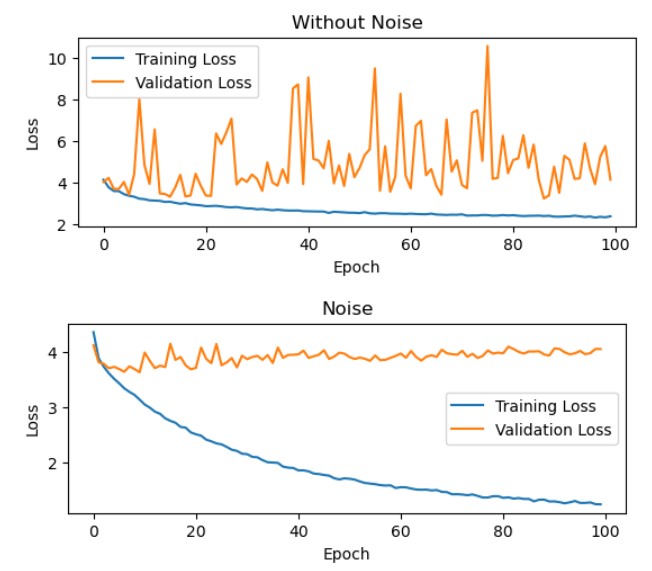
Figure 5: EffectofNoise

4.1.2   Effect of Convolutional Depth

Increase in convolutional depth up to a certain number, increased the model performance where after any further increase resulted in overfitting with large amount of trainable parameters. It should also be noted that model with less convolutions converged faster. This is because lower it has not enough trainable parameters.

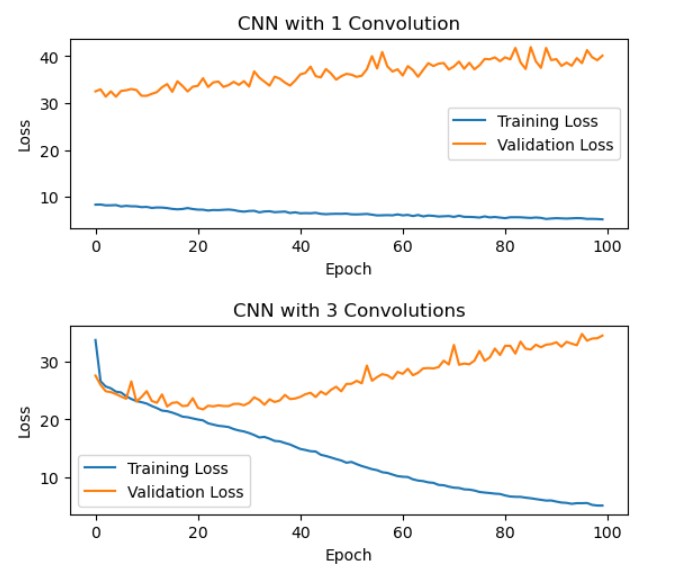
Figure 6: Effect of Convolutional Depth

4.1.3   Effect of Loss Function

Loss function quantifies the discrepancy between the predicted outputs and the actual, and then the model tries to minimize this loss during training. Loss function has effect on how the model parameters are updated after each batch. Different loss functions emphasize different aspects of the training process, such as accuracy, robustness to outliers, or handling class imbalance Root Mean Square Error (RMSE), Mean Absolute Error (MAE), Huber and Log-Cosh loss were tested. and then, MAE was selected as the loss function for further use. This resulted in lower loss, also gave an indication for magnitude of error in the model predictions as it is more interpretable. MAE measures the average absolute difference between the predicted values and the true values and is also less susceptible to outliers which was desirable in our case. MAE is given by the formula:

$$\text{MAE}(y,\hat{y})=\frac{\sum_{i=0}^{N-1}|y_{i}-\hat{y}_{i}|}{N}$$ (5)

4.2   Models Performances

The performance of models were tested through a series of steps. Initially, models ability to learn through data was known through observing training and testing loss. Second evaluation was to test the prediction of model on unseen data. A test set with waveform samples generated through the same simulator were used to evaluating model performance. Then, another test set generated from another LiDAR simulator with different parameters, was used to further evaluate models performance. Finally, real LiDAR data from bathymetric survey, in Northern coastal area of Brittany, was used to evaluate the model.

Results of model’s performance on unseen simulated data are discussed below. The following tables present model performance for prediction of depth of water. Each of better performing model type were tested for predicting the other two parameters. Same Model did not have same performance for each parameter. Though the input is same for predicting each parameter, different parameter learning is required for predicting different parameters.

4.2.1   CNN

1D Convolutional Network showed the best results for predicting the three parameters. A number of experiments were performed by changing the convolutional depth, pooling and filters. Table 2 illustrates performance of CNN models for predicting depth parameter.

Type	Training Loss	Validation Loss	r2 score (t)	r2 score (v)	r2 score	RMSE
Conv1D 1	2.209	4.479	-	-	-	-
– 1D 3	1.041	3.6864	-	-	-	-
– 1D 5	0.613	3.95	0.923	0.314	0.479	1.502
– 1D 5+2D	2.284	2.522	0.591	0.582	0.577
– 1D 9	1.296	3.25	-	-	-	-
– 20 Up	2.661	3.270	0.782	0.184	0.175	2.531
– 20 Down	1.096	2.120	0.514	0.310	0.302	3.785

Table 2: Convolutional Neural Network Models Performance

4.2.2   RNN

Recurrent Neural Network were supposed to be more relevant for dealing with sequential data, yet CNN outclassed slightly for this task. RNN models though not the best but still they showed promising results. Among the RNN models, Attention based models were the most significant in terms of performance metrics.

Type	Training Loss	Validation Loss	r2 score (t)	r2 score (v)	r2 score	RMSE
RNN LSTM 1	4.7868	4.7451	-	-	-	-
LSTM 4	3.6405	3.606	0.0025	0.002	0.002	-
Bidirectional	4.783	4.7467	0.0021	0.0021	0.0028	-
GRU	4.7088	4.6288	0.0002	0.0001	0.007	-
Attention Based	3.114	3.134	0.402	0.383	0.35	4.199

Table 3: Recurrent Neural Network performance

4.2.3   Machine Learning Models

Machine Learning models were not able to predict the parameters to acceptable level. Also, interpretability was not a priority in such case were ML model were not able to provide comparable results.

Type	Training Loss	Validation Loss	r2 score (t)	r2 score (v)	r2 score	RMSE
SVM Linear	-	-	0.715	4e-10	347e-10	-
SVM Polynomial	-	-	-	9e-10	-	-
SVM rbf	-	-	1973e-10	8e-7	-	-
SVM sigmoid	-	-	-	6e-10	6071e-10	-
Random Forest	-	-	-	3975e-10	-	-

Table 4: Machine Learning models

4.2.4   Other Models

Several other models which were originally designed for solving other tasks such as Image classification, SONAR wave parameter predictions, and diffusion were modified and made to predict parameters using waveform as input. However, none of such models, which were tested, were able to make significant improvement than already used models. Table 5 shows tested models with their performance metrics.

Type	Training Loss	Validation Loss	r2 score (t)	r2 score (v)	r2 score	RMSE
Resnet-50	3.064	3.169	0.399	0.350	0.296	3.930
1D soat waveform	0.973	3.745	0.754	0.175	0.124	-
Transformers	0.87	3.2	0.896	0.351	0.381	-
Wavenet	-	-	-	2.15E-11	4.15E-15	-

Table 5: Pre-trained and pre-developed models

4.3   Real LiDAR Data

Bathymetric LiDAR survey data was available for the study area in las format. Initially processing was done using the open source library available at (https://github.com/p-leroy/lidar_platform). For visualization and processing of LiDAR data, Cloud Compare 2.11 was used in addition to python environment. Cloud compare provides 3D visualization of point cloud and FWL data. FWL data is computationally expensive as well as it takes large storage and takes more time for processing. Specialized processing capabilities was required for full waveform. The data contained following attributes

• intensity

• return number

• number of returns

• classification

• user data

• scan direction flag

• point source id

• gps time

• wavepacket index

• wavepacket offset

• wavepacket size

• return point wave location

• x (t)

• y (t)

• z (t)

• XYZ

• depth

• metadata

Full waveform were available in a seperate file in wdp format. The number of waveforms avaialble were 30519 while time stamps were 168. After preprocessing, the shape of LiDAR data was (30519, 512, 1). The space required for storing these waveforms, stand alone file, was 8 Gigabytes.

For selection of points that did not belong to surface of water, 3D visualziation in Cloud Compare was used to segment out such points. A clear distinction between surface and sea bed points were observed. To further enhance the contrast, points were given color on basis of depth.

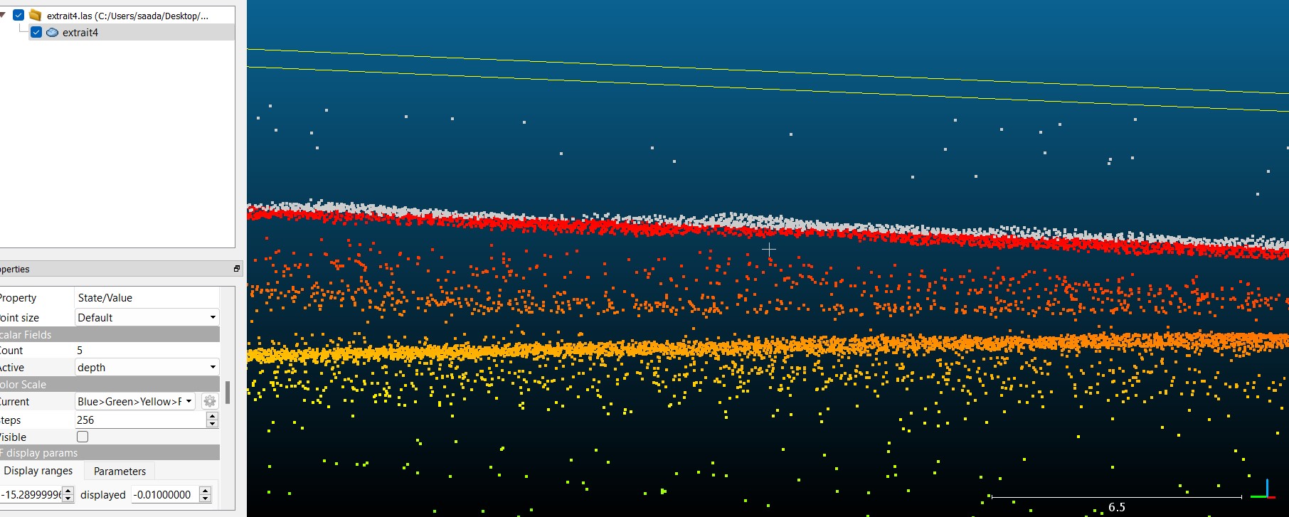
Figure 7: Difference between Surface and Sea-bed points

Figure 7 shows visualization of real LiDAR data. The two layers that are dominant in figure. The upper one shows the surface reflectance while the lower one is the sea bed. Other points in between are reflectance from within the water column.

4.4   Kd Estimation

The attenuation coefficient of water (Kd) refers to the measure of the reduction in the intensity of an electromagnetic wave as it passes through water. It quantifies how quickly the energy of the wave is absorbed, scattered, or dispersed within the water medium. The coefficient is influenced by various factors such as the frequency of the wave, water temperature, salinity, and the presence of impurities or suspended particles in the water. In general, shorter wavelengths (e.g., blue or green light) tend to be absorbed more, while longer wavelengths (e.g., red or infrared light) are scattered more. This behavior affects the penetration depth of light in water

Measuring Kd provides valuable information about the strength of molecular interactions, aiding in drug discovery, understanding biological processes, and optimizing molecular interactions. Hence, it is important to know about kd.

Estimation is a tricky process as it does not vary much on a small spatial scale especially in oceans. The value of kd varies from 0.05 to 3.6 $m^{-1}$ (Corcoran  Parrish, 2021). Spatial variability of kd in the study area was observed not to be changing rapidly. To get the kd value for an area, one has to do regression of intensity and depth. The log of intensity was plot with depth can be shown in the figure,

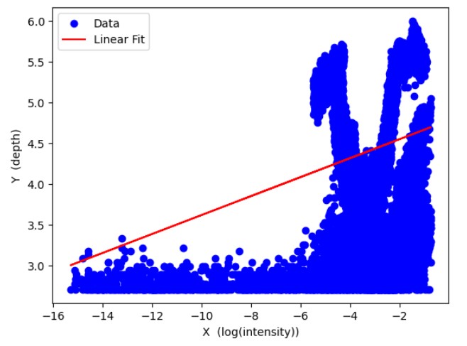
Figure 8: Attenuation coefficient assessment through Regression

The slope of the red line in figure 8 gives the approximation of Attenuation coefficient (kd) value. This is the only way to determine the value of attenuation coefficient without use of deep learning. Similar regression analysis were made for 3 other real LiDAR data-sets available for having a reference kd value. It is to be noted that, the slope of line is a single value that is a generalized value for all the data points within the plot. There is no available means, to have individual kd values for each waveform without deep learning method. In the plot 8, slope of linear fit line was 0.2323 which was selected as the ground truth value for kd.

4.4.1   Model with Best Performance

With rigorous testing, a CNN model was selected as best performing model. There were three methods to compile the final model that would predict three parameters. First was to have a single network with three filters in the last layer so to predict three outputs, other way was to have learn feature maps jointly and to have three fully connected layers. The third approach was to have three seperate branches for three types of predictions with same input. All three approaches were tested, the network with three branches performed the best and was selected as the final model.

The model had three branches for predicting three parameters. The three branches had the same input that was waveforms. The three branches were compiled into a single giant model. This was the final model that had the total number of parameters: 5,068,233, trainable parameters: 5,049,993 and non-trainable parameters: 18,240. Figure 9 presents an abstraction of model waveform being processed through the neural network.

Figure 9: Model Summary Sketch

Following table provides performance of the final model after testing through unseen data. This means that the model’s effectiveness and accuracy were assessed on data that it had not been exposed to during its training or validation stages. The table offers insights into how well the model generalizes to new, unseen data, providing a comprehensive assessment of its performance in real-world scenarios. Table 6 presents the metrics for the best performing model which had the lowest error and highest r2 score on simulated data.

Parameter	Training	Validation	Training R2 score	Validation R2 score	Test R2 score	RMSE
depth	2.06	2.069	0.6617	0.6489	0.6518	3.185
kd	0.0252	0.0264	0.9565	0.9541	0.9506	0.0644
bottom	16.74	16.82	0.389	0.374	0.367	22.76

Table 6: Best performing model

Type	MAE	RMSE
depth
trained network	3.895	4.69
domain adaptation	5.485	6.486
fine tuning	1.006	1.4514
kd
trained network	0.2411	0.2949
domain adaptation	0.2718	0.3366
fine tuning	0.2911	0.3395
bottom
trained network	32.03	34.93
domain adaptation	46.031	46.031

Table 7: Performance on other simulated data

Type	MAE	RMSE
depth
trained network	4.49	4.9
domain adaptation	2.319	2.779
fine tuning	1.616	2.1
kd
trained network	0.3674	0.3713
domain adaptation	0.0358	0.0402
fine tuning	0.0358	0.0358

Table 8: Performance on real data

The model exhibited favorable performance when applied to previously unseen data. Model performance was excellent for the test simulated data it was trained on. A slight decrease in performance of model was observed when predictions were made on simulated data and real LiDAR data. Therefore, techniques such as domain adaptation and transfer learning were used. Different domain adaptation and transfer learning technqiues were experimented with. The aforementioned results pertain to the better performing models. The performance of the model increased significantly on real LiDAR data after domain adaptation and fine tuning.

5   Conclusion

One Dimensional Convolution based Neural Network was successfully able to produce a data-driven approximation of the implicit relation between waveform and parameters. This model is first of its kind, it will enhance the usability of Full Waveform LiDAR (FWF) by adding important parameters to bathymetry through LiDAR. A total of one Million simulated waveforms, which were generated using simulator, were used for training of deep learning model. Proposed model showed exceptionally high performance in predicting attenuation coefficient (kd) with correaltion coefficient of 0.95 and loss of 0.028 for test data. Significantly good predictions were made by the model for depth parameter. The model was not able to show high correlation for bottom reflectance in which there is further room for improvement. It is one of the most challenging parameters to predict since, little or no clear signal can be observed in most cases for bottom reflectance. Nevertheless, predictions made by the model are still useful for having an approximate of the bottom reflectance.

Future perspective include making feature space using real LiDAR data with autoencoder network, and then using optimal transport with the feature space instead of transferring real LiDAR data to original waveform space. This technique, in most cases, tends to works better. With availability of more data in future, more robust models can be trained with no further need of domain adaptation for data with different characteristics.

Appendix A Appendix

Following figure shows the displacement of ground height in the study area with respect to mean sea-level from 2016 to 2021. European Ground motion Service, a product by Copernicus, was used for the figure 10.

Figure 10: Time series

Certin parts within study area shows significant and consistent lowering in height per year.

Figure 11: Time series for Temperature with Landsat data

The Gulf of Morbihan (French: Golfe du Morbihan) is a natural harbor located on the southern coast of Brittany in northwestern France. It has a large inlet of the Atlantic Ocean, bordered by the mainland to the north and the Rhuys Peninsula to the south. It covers an area of about 100 square kilometers and is characterized by a labyrinth of small islands, islets, and peninsulas. University of South Brittany is located near to this region. Penestin is a commune located in the department of Morbihan. It has golden sandy beaches, coastal landscapes, and rugged cliffs. Field trip to these places were arranged during the research. Being near, these places were best fit for understanding coastal dynamics with respect to LiDAR and Bathymetric surveys.

Figure 12: Field Trip to Penestin and Gulf of Morbihan

The following figure shows the bathymetric map with the path followed by the boat for carrying out survey in Gulf Du Morbihan. The depth of ocean varies between 0 to 30 meters within the region. The shades of blue refers to depth of water.

Bathymetric surveys are costly. The seismic sensor alone costed eighty thousand euros. Seismic sensors used in bathymetric surveys are specialized instruments designed to measure the depth of water and map the underwater topography. These sensors use sound waves or acoustic signals to determine the water depth by measuring the time it takes for the signal to bounce back from the seafloor. This information is then used to create detailed bathymetric maps. Bathymetric surveys involve additional costs apart from the seismic sensor itself. These costs include the deployment and operation of survey vessels, data processing and analysis, calibration and maintenance of equipment, and compliance with regulatory requirements. All of these factors contribute to the overall costliness of bathymetric surveys. While bathymetric surveys can be expensive, they provide critical data for various applications, including marine navigation, coastal engineering, resource exploration, and environmental monitoring.

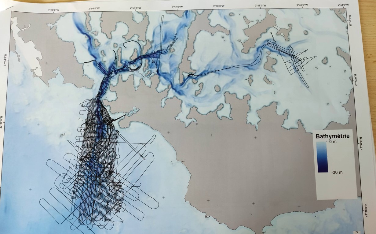
Figure 13: Bathymetric Map Gulf of Morbihan

Figure 14 shows the bathymetry of a channel. The top layer refers to surface of water while subsiding layer below is the sea bed. The interment layer is due to phenomena known as double reflectance.

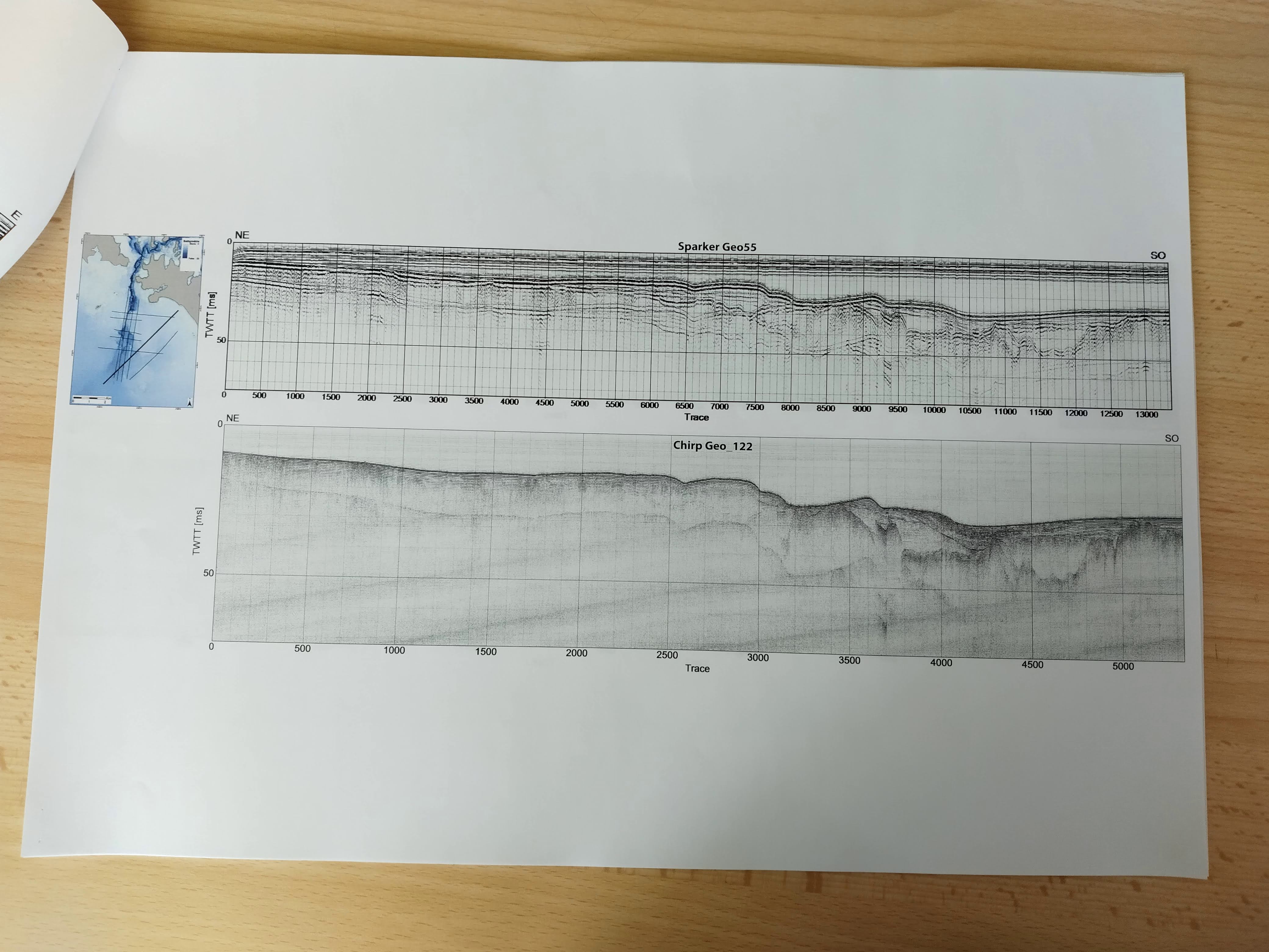
Figure 14: Bathymetric Map showing Surface and Sea-Bed

Figure 15 shows Bathymetric Map generated through survey for Gulf of Morbihan.

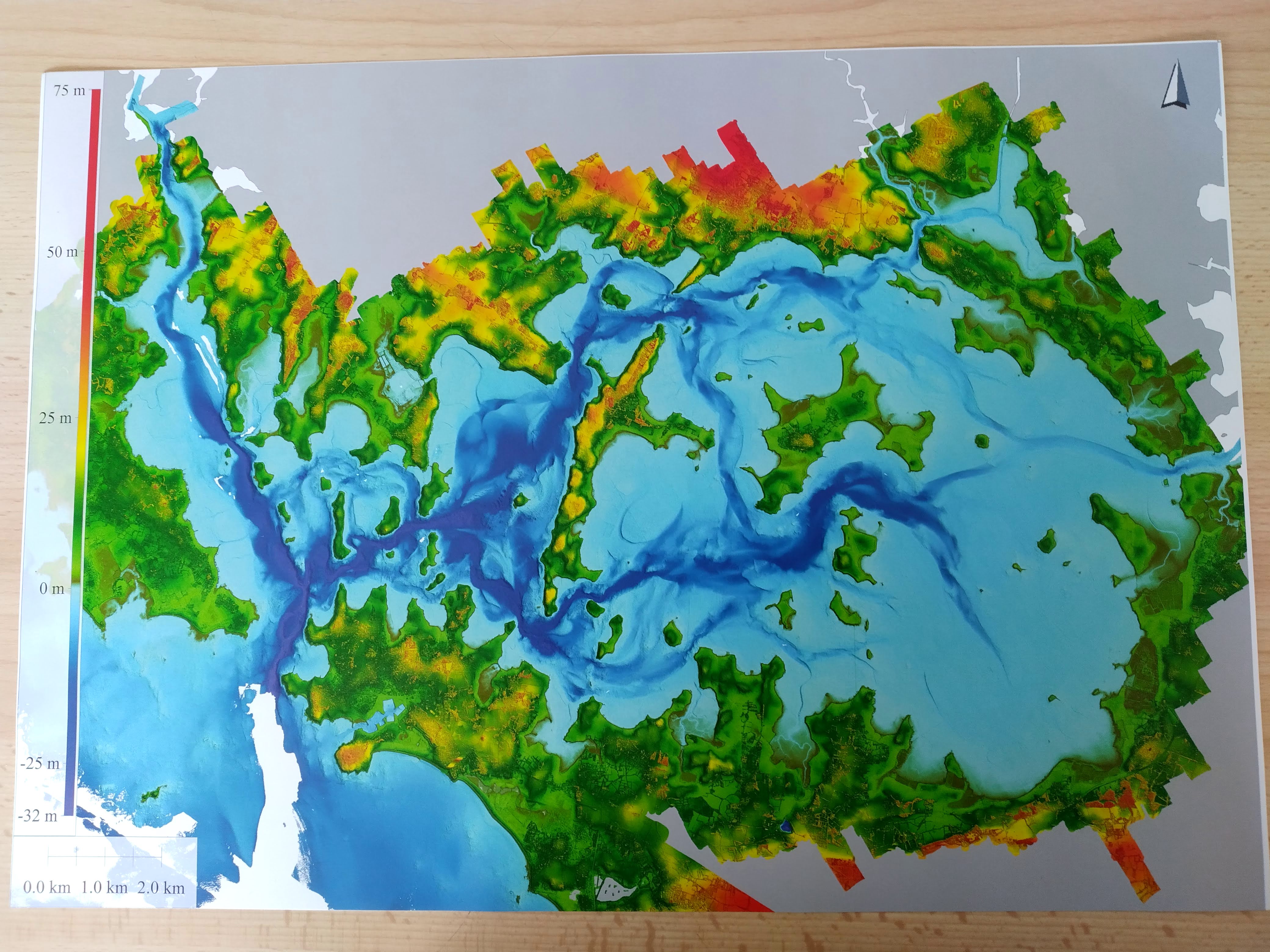
Figure 15: Bathymetric Map

CloudCompare is an open-source software for LiDAR data processing and visualization. It provides a wide range of functionalities for working with point cloud or full waveform data.

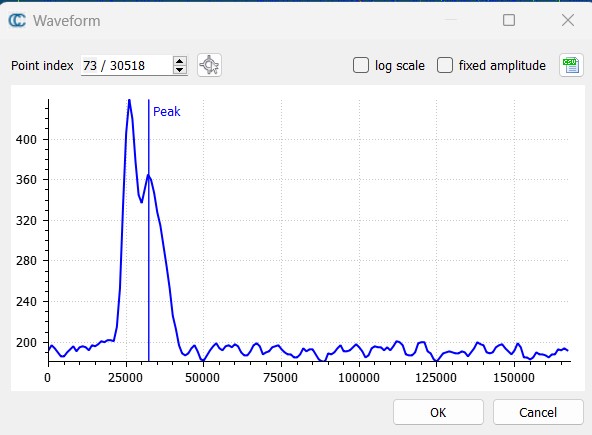
Figure 16: Visualization of Full Waveform in Cloud Compare

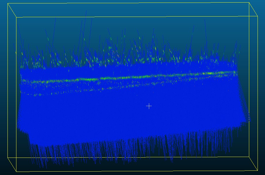
Figure 17: Real LiDAR Full Waveform Data Visualization

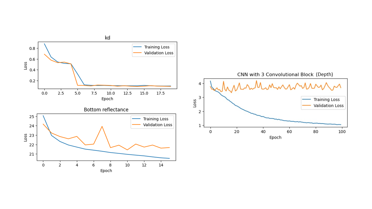
Figure 18: Learning Curve during Training for parameters

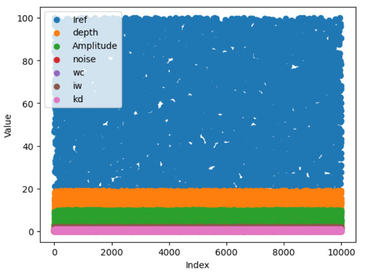
Figure 19: Scatter plot for spread of simulator parameters

Figure 20: Histogram for real LiDAR data

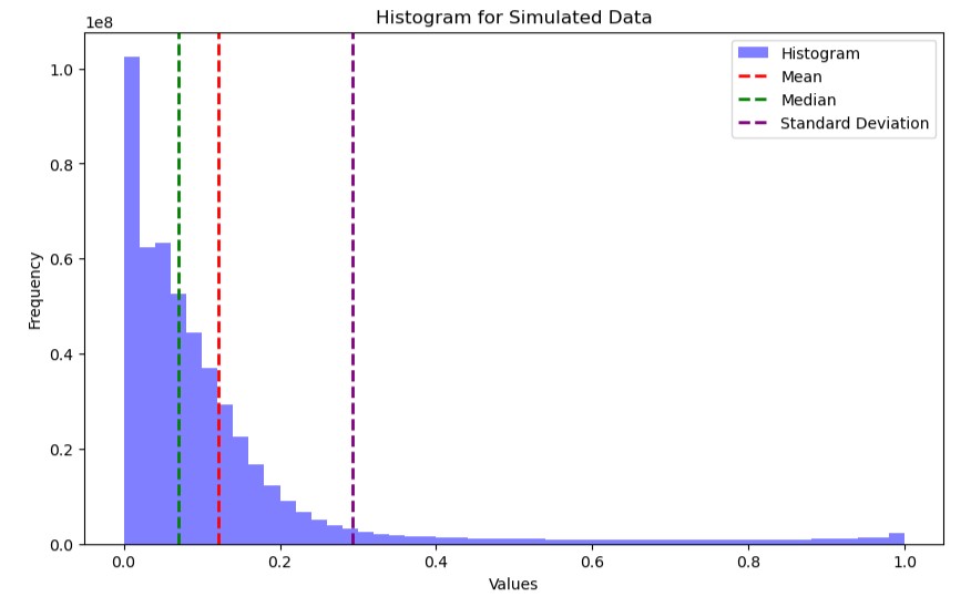
Figure 21: Histogram for simulated data

…

Declaration

I hereby declare that I have completed the present work independently and made without the use of any aids other than those specified. All Bodies that come literally or analogously from published and unpublished Scripts were taken are marked as such. I certify that the submitted electronic version fully corresponds to the printed version submitted.


Salzburg, 15.06.2023

————————
Saad Ahmed Jamal

Declaration of consent for plagiarism check

Name:	Jamal
First name:	Saad Ahmed
Degree:	Master
Student ID:	s1085493

I hereby agree that, Prof. Dr. Dirk Tiede, master’s thesis submitted to plagiarism checking tools can be subjected to automated plagiarism checking.

The work is checked exclusively and will only take place anonymously and without permanent storage in the database of the plagiarism check tool.

It has been pointed out to me that a result of the plagiarism check that indicates the use of external, unidentified sources represents an attempt at deception. In this case, the work is evaluated as a failed examination. Further measures relating to examination law or criminal law can be initiated in consultation with the examination office.


Salzburg, 15.06.2023

————————
Saad Ahmed Jamal

References

- Abdallah \BOthers. (\APACyear2012) \APACinsertmetastarwalid{APACrefauthors}Abdallah, H., Baghdadi, N., Bailly\BCBL \BBA Fabre, F. \APACrefYearMonthDay2012. \BBOQ\APACrefatitleWa-LiD: A New LiDAR Simulator for Waters Wa-lid: A new lidar simulator for waters.\BBCQ \APACjournalVolNumPagesIEEE Geoscience and Remote Sensing Letters94744–748. {APACrefDOI} \doi10.1109/LGRS.2011.2180506 \PrintBackRefs\CurrentBib
- Alzubaidi \BOthers. (\APACyear2021) \APACinsertmetastarAlzubaidi_2021{APACrefauthors}Alzubaidi, L., Zhang, J., Humaidi, A\BPBIJ., Al-Dujaili, A., Duan, Y., Al-Shamma, O.\BDBLFarhan, L. \APACrefYearMonthDay2021mar. \BBOQ\APACrefatitleReview of deep learning: concepts, CNN architectures, challenges, applications, future directions Review of deep learning: concepts, cnn architectures, challenges, applications, future directions.\BBCQ \APACjournalVolNumPagesJournal of Big Data81. {APACrefURL} https://doi.org/10.1186%2Fs40537-021-00444-8 {APACrefDOI} \doi10.1186/s40537-021-00444-8 \PrintBackRefs\CurrentBib
- Andersen \BOthers. (\APACyear2005) \APACinsertmetastarANDERSEN2005441{APACrefauthors}Andersen, H\BHBIE., McGaughey, R\BPBIJ.\BCBL \BBA Reutebuch, S\BPBIE. \APACrefYearMonthDay2005. \BBOQ\APACrefatitleEstimating forest canopy fuel parameters using LIDAR data Estimating forest canopy fuel parameters using lidar data.\BBCQ \APACjournalVolNumPagesRemote Sensing of Environment944441-449. {APACrefURL} https://www.sciencedirect.com/science/article/pii/S0034425704003438 {APACrefDOI} \doihttps://doi.org/10.1016/j.rse.2004.10.013 \PrintBackRefs\CurrentBib
- Awadallah \BOthers. (\APACyear2023) \APACinsertmetastarNewTest_rs15010263{APACrefauthors}Awadallah, M\BPBIO\BPBIM., Malmquist, C., Stickler, M.\BCBL \BBA Alfredsen, K. \APACrefYearMonthDay2023. \BBOQ\APACrefatitleQuantitative Evaluation of Bathymetric LiDAR Sensors and Acquisition Approaches in Lærdal River in Norway Quantitative evaluation of bathymetric lidar sensors and acquisition approaches in lærdal river in norway.\BBCQ \APACjournalVolNumPagesRemote Sensing151. {APACrefURL} https://www.mdpi.com/2072-4292/15/1/263 {APACrefDOI} \doi10.3390/rs15010263 \PrintBackRefs\CurrentBib
- Aßmann \BOthers. (\APACyear2021) \APACinsertmetastarSimulator2{APACrefauthors}Aßmann, A., Stewart, B.\BCBL \BBA Wallace, A\BPBIM. \APACrefYearMonthDay2021. \BBOQ\APACrefatitleDeep Learning for LiDAR Waveforms with Multiple Returns Deep learning for lidar waveforms with multiple returns.\BBCQ \BIn \APACrefbtitle28th European Signal Processing Conference (EUSIPCO) 28th european signal processing conference (eusipco) (\BPG 1571-1575). {APACrefDOI} \doi10.23919/Eusipco47968.2020.9287545 \PrintBackRefs\CurrentBib
- Baghdadi \BOthers. (\APACyear2011) \APACinsertmetastarBaghdadi_2011{APACrefauthors}Baghdadi, N., Lemarquand, N., Abdallah, H.\BCBL \BBA Bailly, J\BPBIS. \APACrefYearMonthDay2011apr. \BBOQ\APACrefatitleThe Relevance of GLAS/ICESat Elevation Data for the Monitoring of River Networks The relevance of GLAS/ICESat elevation data for the monitoring of river networks.\BBCQ \APACjournalVolNumPagesRemote Sensing34708–720. {APACrefURL} https://doi.org/10.3390%2Frs3040708 {APACrefDOI} \doi10.3390/rs3040708 \PrintBackRefs\CurrentBib
- E. Baltsavias (\APACyear1999) \APACinsertmetastarReview2BALTSAVIAS1999199{APACrefauthors}Baltsavias, E. \APACrefYearMonthDay1999. \BBOQ\APACrefatitleAirborne laser scanning: basic relations and formulas Airborne laser scanning: basic relations and formulas.\BBCQ \APACjournalVolNumPagesISPRS Journal of Photogrammetry and Remote Sensing542199-214. {APACrefURL} https://www.sciencedirect.com/science/article/pii/S0924271699000155 {APACrefDOI} \doihttps://doi.org/10.1016/S0924-2716(99)00015-5 \PrintBackRefs\CurrentBib
- E\BPBIP. Baltsavias (\APACyear1999) \APACinsertmetastarReviewBALTSAVIAS199983{APACrefauthors}Baltsavias, E\BPBIP. \APACrefYearMonthDay1999. \BBOQ\APACrefatitleA comparison between photogrammetry and laser scanning A comparison between photogrammetry and laser scanning.\BBCQ \APACjournalVolNumPagesISPRS Journal of Photogrammetry and Remote Sensing54283-94. {APACrefURL} https://www.sciencedirect.com/science/article/pii/S0924271699000143 {APACrefDOI} \doihttps://doi.org/10.1016/S0924-2716(99)00014-3 \PrintBackRefs\CurrentBib
- Beland \BOthers. (\APACyear2019) \APACinsertmetastarBELAND2019117484{APACrefauthors}Beland, M., Parker, G., Sparrow, B., Harding, D., Chasmer, L., Phinn, S.\BDBLStrahler, A. \APACrefYearMonthDay2019. \BBOQ\APACrefatitleOn promoting the use of lidar systems in forest ecosystem research On promoting the use of lidar systems in forest ecosystem research.\BBCQ \APACjournalVolNumPagesForest Ecology and Management450117484. {APACrefURL} https://www.sciencedirect.com/science/article/pii/S0378112719306218 {APACrefDOI} \doihttps://doi.org/10.1016/j.foreco.2019.117484 \PrintBackRefs\CurrentBib
- Bishop (\APACyear1995) \APACinsertmetastarNoise_10.1162/neco.1995.7.1.108{APACrefauthors}Bishop, C\BPBIM. \APACrefYearMonthDay199501. \BBOQ\APACrefatitleTraining with Noise is Equivalent to Tikhonov Regularization Training with Noise is Equivalent to Tikhonov Regularization.\BBCQ \APACjournalVolNumPagesNeural Computation71108-116. {APACrefURL} https://doi.org/10.1162/neco.1995.7.1.108 {APACrefDOI} \doi10.1162/neco.1995.7.1.108 \PrintBackRefs\CurrentBib
- Brynjarsdóttir \BBA O’Hagan (\APACyear2014) \APACinsertmetastarBrynjarsdottir_2014{APACrefauthors}Brynjarsdóttir, J.\BCBT \BBA O’Hagan, A. \APACrefYearMonthDay2014oct. \BBOQ\APACrefatitleLearning about physical parameters: the importance of model discrepancy Learning about physical parameters: the importance of model discrepancy.\BBCQ \APACjournalVolNumPagesInverse Problems3011114007. {APACrefURL} https://dx.doi.org/10.1088/0266-5611/30/11/114007 {APACrefDOI} \doi10.1088/0266-5611/30/11/114007 \PrintBackRefs\CurrentBib
- Calderón-Macías \BOthers. (\APACyear2000) \APACinsertmetastarCalder_n_Mac_as_2000{APACrefauthors}Calderón-Macías, C., Sen, M\BPBIK.\BCBL \BBA Stoffa, P\BPBIL. \APACrefYearMonthDay2000jan. \BBOQ\APACrefatitleArtificial neural networks for parameter estimation in geophysics Artificial neural networks for parameter estimation in geophysics.\BBCQ \APACjournalVolNumPagesGeophysical Prospecting48121–47. {APACrefURL} https://doi.org/10.1046%2Fj.1365-2478.2000.00171.x {APACrefDOI} \doi10.1046/j.1365-2478.2000.00171.x \PrintBackRefs\CurrentBib
- Chen \BOthers. (\APACyear2022) \APACinsertmetastarChen_2022{APACrefauthors}Chen, C., Jin, A., Yang, B., Ma, R., Sun, S., Wang, Z.\BDBLZhang, F. \APACrefYearMonthDay2022aug. \BBOQ\APACrefatitleDCPLD-Net: A diffusion coupled convolution neural network for real-time power transmission lines detection from UAV-Borne LiDAR data DCPLD-net: A diffusion coupled convolution neural network for real-time power transmission lines detection from UAV-borne LiDAR data.\BBCQ \APACjournalVolNumPagesInternational Journal of Applied Earth Observation and Geoinformation112102960. {APACrefURL} https://doi.org/10.1016%2Fj.jag.2022.102960 {APACrefDOI} \doi10.1016/j.jag.2022.102960 \PrintBackRefs\CurrentBib
- Chust \BOthers. (\APACyear2010) \APACinsertmetastarCHUST2010200{APACrefauthors}Chust, G., Grande, M., Galparsoro, I., Uriarte, A.\BCBL \BBA Ángel Borja. \APACrefYearMonthDay2010. \BBOQ\APACrefatitleCapabilities of the bathymetric Hawk Eye LiDAR for coastal habitat mapping: A case study within a Basque estuary Capabilities of the bathymetric hawk eye lidar for coastal habitat mapping: A case study within a basque estuary.\BBCQ \APACjournalVolNumPagesEstuarine, Coastal and Shelf Science893200–213. {APACrefURL} https://www.sciencedirect.com/science/article/pii/S0272771410002477 {APACrefDOI} \doihttps://doi.org/10.1016/j.ecss.2010.07.002 \PrintBackRefs\CurrentBib
- Corcoran \BBA Parrish (\APACyear2021) \APACinsertmetastarCorcoran_2021{APACrefauthors}Corcoran, F.\BCBT \BBA Parrish, C\BPBIE. \APACrefYearMonthDay2021nov. \BBOQ\APACrefatitleDiffuse Attenuation Coefficient (Kd) from ICESat-2 ATLAS Spaceborne Lidar Using Random-Forest Regression Diffuse attenuation coefficient (kd) from icesat-2 atlas spaceborne lidar using random-forest regression.\BBCQ \APACjournalVolNumPagesPhotogrammetric Engineering and Remote Sensing8711831–840. {APACrefURL} https://doi.org/10.14358%2Fpers.21-00013r2 {APACrefDOI} \doi10.14358/pers.21-00013r2 \PrintBackRefs\CurrentBib
- Courty \BOthers. (\APACyear2017) \APACinsertmetastarCourty_758603{APACrefauthors}Courty, N., Flamary, R., Tuia, D.\BCBL \BBA Rakotomamonjy, A. \APACrefYearMonthDay2017. \BBOQ\APACrefatitleOptimal Transport for Domain Adaptation Optimal transport for domain adaptation.\BBCQ \APACjournalVolNumPagesIEEE Transactions on Pattern Analysis and Machine Intelligence3991853-1865. {APACrefDOI} \doi10.1109/TPAMI.2016.2615921 \PrintBackRefs\CurrentBib
- Deems \BOthers. (\APACyear2013) \APACinsertmetastardeems_painter_finnegan_2013{APACrefauthors}Deems, J\BPBIS., Painter, T\BPBIH.\BCBL \BBA Finnegan, D\BPBIC. \APACrefYearMonthDay2013. \BBOQ\APACrefatitleLidar measurement of snow depth: a review Lidar measurement of snow depth: a review.\BBCQ \APACjournalVolNumPagesJournal of Glaciology59215467–479. {APACrefDOI} \doi10.3189/2013JoG12J154 \PrintBackRefs\CurrentBib
- Fairfield \BBA Wettergreen (\APACyear2008) \APACinsertmetastarConference_5151853{APACrefauthors}Fairfield, N.\BCBT \BBA Wettergreen, D. \APACrefYearMonthDay2008. \BBOQ\APACrefatitleActive localization on the ocean floor with multibeam sonar Active localization on the ocean floor with multibeam sonar.\BBCQ \BIn \APACrefbtitleOCEANS 2008 Oceans 2008 (\BPG 1-10). {APACrefDOI} \doi10.1109/OCEANS.2008.5151853 \PrintBackRefs\CurrentBib
- Farahani \BOthers. (\APACyear2020) \APACinsertmetastarDBLP:journals/corr/abs-2010-03978{APACrefauthors}Farahani, A., Voghoei, S., Rasheed, K.\BCBL \BBA Arabnia, H\BPBIR. \APACrefYearMonthDay2020. \BBOQ\APACrefatitleA Brief Review of Domain Adaptation A brief review of domain adaptation.\BBCQ \APACjournalVolNumPagesCoRRabs/2010.03978. {APACrefURL} https://arxiv.org/abs/2010.03978 \PrintBackRefs\CurrentBib
- Guiotte \BOthers. (\APACyear2020) \APACinsertmetastar8954886{APACrefauthors}Guiotte, F., Pham, M\BHBIT., Dambreville, R., Corpetti, T.\BCBL \BBA Lefèvre, S. \APACrefYearMonthDay2020. \BBOQ\APACrefatitleSemantic Segmentation of LiDAR Points Clouds: Rasterization Beyond Digital Elevation Models Semantic segmentation of lidar points clouds: Rasterization beyond digital elevation models.\BBCQ \APACjournalVolNumPagesIEEE Geoscience and Remote Sensing Letters17112016–2019. {APACrefDOI} \doi10.1109/LGRS.2019.2958858 \PrintBackRefs\CurrentBib
- Heinzel \BBA Koch (\APACyear2011) \APACinsertmetastarHEINZEL2011152{APACrefauthors}Heinzel, J.\BCBT \BBA Koch, B. \APACrefYearMonthDay2011. \BBOQ\APACrefatitleExploring full-waveform LiDAR parameters for tree species classification Exploring full-waveform lidar parameters for tree species classification.\BBCQ \APACjournalVolNumPagesInternational Journal of Applied Earth Observation and Geoinformation131152-160. {APACrefURL} https://www.sciencedirect.com/science/article/pii/S0303243410001145 {APACrefDOI} \doihttps://doi.org/10.1016/j.jag.2010.09.010 \PrintBackRefs\CurrentBib
- Islam \BOthers. (\APACyear2022) \APACinsertmetastareast_pak{APACrefauthors}Islam, M\BPBIT., Yoshida, K., Nishiyama, S., Sakai, K.\BCBL \BBA Tsuda, T. \APACrefYearMonthDay2022. \BBOQ\APACrefatitleCharacterizing vegetated rivers using novel unmanned aerial vehicle-borne topo-bathymetric green lidar: Seasonal applications and challenges Characterizing vegetated rivers using novel unmanned aerial vehicle-borne topo-bathymetric green lidar: Seasonal applications and challenges.\BBCQ \APACjournalVolNumPagesRiver Research and Applications38144-58. {APACrefURL} https://onlinelibrary.wiley.com/doi/abs/10.1002/rra.3875 {APACrefDOI} \doihttps://doi.org/10.1002/rra.3875 \PrintBackRefs\CurrentBib
- Jamal \BBA Aribisala (\APACyear2023) \APACinsertmetastarjamal2023data{APACrefauthors}Jamal, S\BPBIA.\BCBT \BBA Aribisala, A. \APACrefYearMonthDay2023. \APACrefbtitleData Fusion for Multi-Task Learning of Building Extraction and Height Estimation. Data fusion for multi-task learning of building extraction and height estimation. {APACrefURL} https://doi.org/10.48550/arXiv.2308.02960 {APACrefDOI} \doi10.48550/arXiv.2308.02960 \PrintBackRefs\CurrentBib
- Koetz \BOthers. (\APACyear2006) \APACinsertmetastar1576688{APACrefauthors}Koetz, B., Morsdorf, F., Sun, G., Ranson, K., Itten, K.\BCBL \BBA Allgower, B. \APACrefYearMonthDay2006. \BBOQ\APACrefatitleInversion of a lidar waveform model for forest biophysical parameter estimation Inversion of a lidar waveform model for forest biophysical parameter estimation.\BBCQ \APACjournalVolNumPagesIEEE Geoscience and Remote Sensing Letters3149–53. {APACrefDOI} \doi10.1109/LGRS.2005.856706 \PrintBackRefs\CurrentBib
- Lague \BBA Feldmann (\APACyear2020) \APACinsertmetastarLAGUE202025{APACrefauthors}Lague, D.\BCBT \BBA Feldmann, B. \APACrefYearMonthDay2020. \BBOQ\APACrefatitleChapter 2 - Topo-bathymetric airborne LiDAR for fluvial-geomorphology analysis Chapter 2 - topo-bathymetric airborne lidar for fluvial-geomorphology analysis.\BBCQ \BIn P. Tarolli \BBA S\BPBIM. Mudd (\BEDS), \APACrefbtitleRemote Sensing of Geomorphology Remote sensing of geomorphology (\BVOL 23, \BPG 25-54). \APACaddressPublisherElsevier. {APACrefURL} https://www.sciencedirect.com/science/article/pii/B9780444641779000023 {APACrefDOI} \doihttps://doi.org/10.1016/B978-0-444-64177-9.00002-3 \PrintBackRefs\CurrentBib
- Letard, Collin, Corpetti\BCBL \BOthers. (\APACyear2022) \APACinsertmetastarLetard_2022{APACrefauthors}Letard, M., Collin, A., Corpetti, T., Lague, D., Pastol, Y.\BCBL \BBA Ekelund, A. \APACrefYearMonthDay2022jan. \BBOQ\APACrefatitleClassification of Land-Water Continuum Habitats Using Exclusively Airborne Topobathymetric Lidar Green Waveforms and Infrared Intensity Point Clouds Classification of land-water continuum habitats using exclusively airborne topobathymetric lidar green waveforms and infrared intensity point clouds.\BBCQ \APACjournalVolNumPagesRemote Sensing142341. {APACrefURL} https://doi.org/10.3390%2Frs14020341 {APACrefDOI} \doi10.3390/rs14020341 \PrintBackRefs\CurrentBib
- Letard, Collin, Corpetti\BCBL \BOthers. (\APACyear2021) \APACinsertmetastarLetard_Conf_9705797{APACrefauthors}Letard, M., Collin, A., Corpetti, T., Lague, D., Pastol, Y., Gloria, H.\BDBLMury, A. \APACrefYearMonthDay2021. \BBOQ\APACrefatitleClassification of coastal and estuarine ecosystems using full-waveform topo-bathymetric lidar data and artificial intelligence Classification of coastal and estuarine ecosystems using full-waveform topo-bathymetric lidar data and artificial intelligence.\BBCQ \BIn \APACrefbtitleOCEANS 2021: San Diego – Porto Oceans 2021: San diego – porto (\BPG 1-10). {APACrefDOI} \doi10.23919/OCEANS44145.2021.9705797 \PrintBackRefs\CurrentBib
- Letard, Collin, Lague\BCBL \BOthers. (\APACyear2022) \APACinsertmetastarLetard_isprs-archives-XLIII-B3-2022-463-2022{APACrefauthors}Letard, M., Collin, A., Lague, D., Corpetti, T., Pastol, Y.\BCBL \BBA Ekelund, A. \APACrefYearMonthDay2022. \BBOQ\APACrefatitleUSING BISPECTRAL FULL-WAVEFORM LIDAR TO MAP SEAMLESS COASTAL HABITATS IN 3D Using bispectral full-waveform lidar to map seamless coastal habitats in 3d.\BBCQ \APACjournalVolNumPagesThe International Archives of the Photogrammetry, Remote Sensing and Spatial Information SciencesXLIII-B3-2022463–470. {APACrefURL} https://www.int-arch-photogramm-remote-sens-spatial-inf-sci.net/XLIII-B3-2022/463/2022/ {APACrefDOI} \doi10.5194/isprs-archives-XLIII-B3-2022-463-2022 \PrintBackRefs\CurrentBib
- Letard, Collin, Lague\BCBL \BOthers. (\APACyear2021) \APACinsertmetastarLetard9554262{APACrefauthors}Letard, M., Collin, A., Lague, D., Corpetti, T., Pastol, Y., Ekelund, A.\BDBLCosta, S. \APACrefYearMonthDay2021. \BBOQ\APACrefatitleTowards 3D Mapping of Seagrass Meadows with Topo-Bathymetric Lidar Full Waveform Processing Towards 3d mapping of seagrass meadows with topo-bathymetric lidar full waveform processing.\BBCQ \BIn \APACrefbtitle2021 IEEE International Geoscience and Remote Sensing Symposium IGARSS 2021 ieee international geoscience and remote sensing symposium igarss (\BPGS 8069–8072). {APACrefDOI} \doi10.1109/IGARSS47720.2021.9554262 \PrintBackRefs\CurrentBib
- Liao \BOthers. (\APACyear2018) \APACinsertmetastardeeplearning3{APACrefauthors}Liao, W., Van Coillie, F., Gao, L., Li, L., Zhang, B.\BCBL \BBA Chanussot, J. \APACrefYearMonthDay2018. \BBOQ\APACrefatitleDeep Learning for Fusion of APEX Hyperspectral and Full-Waveform LiDAR Remote Sensing Data for Tree Species Mapping Deep learning for fusion of apex hyperspectral and full-waveform lidar remote sensing data for tree species mapping.\BBCQ \APACjournalVolNumPagesIEEE Access668716–68729. {APACrefDOI} \doi10.1109/ACCESS.2018.2880083 \PrintBackRefs\CurrentBib
- Liu \BBA Ke (\APACyear2019) \APACinsertmetastarSuperResolution10.111712.2536719{APACrefauthors}Liu, G.\BCBT \BBA Ke, J. \APACrefYearMonthDay2019. \BBOQ\APACrefatitleDeep-learning for super-resolution full-waveform lidar Deep-learning for super-resolution full-waveform lidar.\BBCQ \BIn Q. Dai, T. Shimura\BCBL \BBA Z. Zheng (\BEDS), \APACrefbtitleOptoelectronic Imaging and Multimedia Technology VI Optoelectronic imaging and multimedia technology vi (\BVOL 11187, \BPG 1118714). \APACaddressPublisherSPIE. {APACrefURL} https://doi.org/10.1117/12.2536719 {APACrefDOI} \doi10.1117/12.2536719 \PrintBackRefs\CurrentBib
- Mallet \BBA Bretar (\APACyear2009) \APACinsertmetastarReview0_MALLET20091{APACrefauthors}Mallet, C.\BCBT \BBA Bretar, F. \APACrefYearMonthDay2009. \BBOQ\APACrefatitleFull-waveform topographic lidar: State-of-the-art Full-waveform topographic lidar: State-of-the-art.\BBCQ \APACjournalVolNumPagesISPRS Journal of Photogrammetry and Remote Sensing6411–16. {APACrefURL} https://www.sciencedirect.com/science/article/pii/S0924271608000993 {APACrefDOI} \doihttps://doi.org/10.1016/j.isprsjprs.2008.09.007 \PrintBackRefs\CurrentBib
- Mallet \BOthers. (\APACyear2011) \APACinsertmetastarMALLET2011S71{APACrefauthors}Mallet, C., Bretar, F., Roux, M., Soergel, U.\BCBL \BBA Heipke, C. \APACrefYearMonthDay2011. \BBOQ\APACrefatitleRelevance assessment of full-waveform lidar data for urban area classification Relevance assessment of full-waveform lidar data for urban area classification.\BBCQ \APACjournalVolNumPagesISPRS Journal of Photogrammetry and Remote Sensing666, SupplementS71-S84. {APACrefURL} https://www.sciencedirect.com/science/article/pii/S0924271611001055 \APACrefnoteAdvances in LIDAR Data Processing and Applications {APACrefDOI} \doihttps://doi.org/10.1016/j.isprsjprs.2011.09.008 \PrintBackRefs\CurrentBib
- Mallet \BOthers. (\APACyear2009) \APACinsertmetastarmallet:hal-02384727{APACrefauthors}Mallet, C., Lafarge, F., Bretar, F., Roux, M., Soergel, U.\BCBL \BBA Heipke, C. \APACrefYearMonthDay2009September. \BBOQ\APACrefatitleA stochastic approach for modelling airborne lidar waveforms A stochastic approach for modelling airborne lidar waveforms.\BBCQ \BIn \APACrefbtitleLaserscanning. Laserscanning. \APACaddressPublisherParis, France. {APACrefURL} https://hal.science/hal-02384727 \PrintBackRefs\CurrentBib
- Maltezos \BOthers. (\APACyear2019) \APACinsertmetastar8465968{APACrefauthors}Maltezos, E., Doulamis, A., Doulamis, N.\BCBL \BBA Ioannidis, C. \APACrefYearMonthDay2019. \BBOQ\APACrefatitleBuilding Extraction From LiDAR Data Applying Deep Convolutional Neural Networks Building extraction from lidar data applying deep convolutional neural networks.\BBCQ \APACjournalVolNumPagesIEEE Geoscience and Remote Sensing Letters161155–159. {APACrefDOI} \doi10.1109/LGRS.2018.2867736 \PrintBackRefs\CurrentBib
- Mandlburger \BOthers. (\APACyear2009) \APACinsertmetastarhess-13-1453-2009{APACrefauthors}Mandlburger, G., Hauer, C., Höfle, B., Habersack, H.\BCBL \BBA Pfeifer, N. \APACrefYearMonthDay2009. \BBOQ\APACrefatitleOptimisation of LiDAR derived terrain models for river flow modelling Optimisation of lidar derived terrain models for river flow modelling.\BBCQ \APACjournalVolNumPagesHydrology and Earth System Sciences1381453–1466. {APACrefURL} https://hess.copernicus.org/articles/13/1453/2009/ {APACrefDOI} \doi10.5194/hess-13-1453-2009 \PrintBackRefs\CurrentBib
- Marinelli \BOthers. (\APACyear2022) \APACinsertmetastar2023_tree_9792315{APACrefauthors}Marinelli, D., Paris, C.\BCBL \BBA Bruzzone, L. \APACrefYearMonthDay2022. \BBOQ\APACrefatitleAn Approach Based on Deep Learning for Tree Species Classification in LiDAR Data Acquired in Mixed Forest An approach based on deep learning for tree species classification in lidar data acquired in mixed forest.\BBCQ \APACjournalVolNumPagesIEEE Geoscience and Remote Sensing Letters191-5. {APACrefDOI} \doi10.1109/LGRS.2022.3181680 \PrintBackRefs\CurrentBib
- Mehendale \BBA Neoge (\APACyear2020) \APACinsertmetastarReview3_Indian_Mehendale_2020{APACrefauthors}Mehendale, N.\BCBT \BBA Neoge, S. \APACrefYearMonthDay2020. \BBOQ\APACrefatitleReview on Lidar Technology Review on lidar technology.\BBCQ \APACjournalVolNumPagesSSRN Electronic Journal. {APACrefURL} https://doi.org/10.2139%2Fssrn.3604309 {APACrefDOI} \doi10.2139/ssrn.3604309 \PrintBackRefs\CurrentBib
- A. Nusrat \BOthers. (\APACyear2022) \APACinsertmetastarnusrat_atmos13020190{APACrefauthors}Nusrat, A., Gabriel, H\BPBIF., e Habiba, U., Rehman, H\BPBIU., Haider, S., Ahmad, S.\BDBLAli, J. \APACrefYearMonthDay2022. \BBOQ\APACrefatitlePlausible Precipitation Trends over the Large River Basins of Pakistan in Twenty First Century Plausible precipitation trends over the large river basins of pakistan in twenty first century.\BBCQ \APACjournalVolNumPagesAtmosphere132. {APACrefURL} https://www.mdpi.com/2073-4433/13/2/190 {APACrefDOI} \doi10.3390/atmos13020190 \PrintBackRefs\CurrentBib
- A. Nusrat \BOthers. (\APACyear2020) \APACinsertmetastarNusrat_2020_app10196878{APACrefauthors}Nusrat, A., Gabriel, H\BPBIF., Haider, S., Ahmad, S., Shahid, M.\BCBL \BBA Ahmed Jamal, S. \APACrefYearMonthDay2020. \BBOQ\APACrefatitleApplication of Machine Learning Techniques to Delineate Homogeneous Climate Zones in River Basins of Pakistan for Hydro-Climatic Change Impact Studies Application of machine learning techniques to delineate homogeneous climate zones in river basins of pakistan for hydro-climatic change impact studies.\BBCQ \APACjournalVolNumPagesApplied Sciences1019. {APACrefURL} https://www.mdpi.com/2076-3417/10/19/6878 {APACrefDOI} \doi10.3390/app10196878 \PrintBackRefs\CurrentBib
- M. Nusrat \BOthers. (\APACyear2023) \APACinsertmetastarosama_unknown{APACrefauthors}Nusrat, M., Habib, Z., Alam, M.\BCBL \BBA Jamal, S\BPBIA. \APACrefYearMonthDay202307. \APACrefbtitleEmoji Prediction in Tweets using BERT. Emoji prediction in tweets using bert. {APACrefURL} https://arxiv.org/abs/2307.02054 {APACrefDOI} \doi10.48550/arXiv.2307.02054 \PrintBackRefs\CurrentBib
- Pelletier \BOthers. (\APACyear2019) \APACinsertmetastarCharlottePelletier_rs11050523{APACrefauthors}Pelletier, C., Webb, G\BPBII.\BCBL \BBA Petitjean, F. \APACrefYearMonthDay2019. \BBOQ\APACrefatitleTemporal Convolutional Neural Network for the Classification of Satellite Image Time Series Temporal convolutional neural network for the classification of satellite image time series.\BBCQ \APACjournalVolNumPagesRemote Sensing115. {APACrefURL} https://www.mdpi.com/2072-4292/11/5/523 {APACrefDOI} \doi10.3390/rs11050523 \PrintBackRefs\CurrentBib
- Raj \BOthers. (\APACyear2020) \APACinsertmetastarRaj_2020{APACrefauthors}Raj, T., Hashim, F\BPBIH., Huddin, A\BPBIB., Ibrahim, M\BPBIF.\BCBL \BBA Hussain, A. \APACrefYearMonthDay2020apr. \BBOQ\APACrefatitleA Survey on LiDAR Scanning Mechanisms A survey on LiDAR scanning mechanisms.\BBCQ \APACjournalVolNumPagesElectronics95741. {APACrefURL} https://doi.org/10.3390%2Felectronics9050741 {APACrefDOI} \doi10.3390/electronics9050741 \PrintBackRefs\CurrentBib
- Szafarczyk \BBA Toś (\APACyear2023) \APACinsertmetastarsurvey4_s23010292{APACrefauthors}Szafarczyk, A.\BCBT \BBA Toś, C. \APACrefYearMonthDay2023. \BBOQ\APACrefatitleThe Use of Green Laser in LiDAR Bathymetry: State of the Art and Recent Advancements The use of green laser in lidar bathymetry: State of the art and recent advancements.\BBCQ \APACjournalVolNumPagesSensors231. {APACrefURL} https://www.mdpi.com/1424-8220/23/1/292 {APACrefDOI} \doi10.3390/s23010292 \PrintBackRefs\CurrentBib
- Wu \BOthers. (\APACyear2018) \APACinsertmetastarGTA-V_8462926{APACrefauthors}Wu, B., Wan, A., Yue, X.\BCBL \BBA Keutzer, K. \APACrefYearMonthDay2018. \BBOQ\APACrefatitleSqueezeSeg: Convolutional Neural Nets with Recurrent CRF for Real-Time Road-Object Segmentation from 3D LiDAR Point Cloud Squeezeseg: Convolutional neural nets with recurrent crf for real-time road-object segmentation from 3d lidar point cloud.\BBCQ \BIn \APACrefbtitle2018 IEEE International Conference on Robotics and Automation (ICRA) 2018 ieee international conference on robotics and automation (icra) (\BPGS 1887–1893). {APACrefDOI} \doi10.1109/ICRA.2018.8462926 \PrintBackRefs\CurrentBib
- Yang \BOthers. (\APACyear2022) \APACinsertmetastarattenuation_photonics9100713{APACrefauthors}Yang, G., Tian, Z., Bi, Z., Cui, Z., Sun, F.\BCBL \BBA Liu, Q. \APACrefYearMonthDay2022. \BBOQ\APACrefatitleMeasurement of the Attenuation Coefficient in Fresh Water Using the Adjacent Frame Difference Method Measurement of the attenuation coefficient in fresh water using the adjacent frame difference method.\BBCQ \APACjournalVolNumPagesPhotonics910. {APACrefURL} https://www.mdpi.com/2304-6732/9/10/713 {APACrefDOI} \doi10.3390/photonics9100713 \PrintBackRefs\CurrentBib
- Zorzi \BOthers. (\APACyear2019) \APACinsertmetastarZorziAustria8737008{APACrefauthors}Zorzi, S., Maset, E., Fusiello, A.\BCBL \BBA Crosilla, F. \APACrefYearMonthDay2019. \BBOQ\APACrefatitleFull-Waveform Airborne LiDAR Data Classification Using Convolutional Neural Networks Full-waveform airborne lidar data classification using convolutional neural networks.\BBCQ \APACjournalVolNumPagesIEEE Transactions on Geoscience and Remote Sensing57108255–8261. {APACrefDOI} \doi10.1109/TGRS.2019.2919472 \PrintBackRefs\CurrentBib