Thermodynamic geometric analysis of 3D charged black holes under f(R) gravity

Abstract

This article investigates 3D charged black holes within the scope of f(R) gravity, focusing on their thermodynamic attributes. The research primarily examines minor fluctuations around these black holes’ equilibrium states and delves into their modified thermodynamic entropy. Utilizing geometric thermodynamics (GTD), the study evaluates the curvature scalar’s role in pinpointing phase transition points in these black holes. A key finding is that several 3D charged black holes under f(R) gravity display thermodynamic properties akin to an ideal gas when their initial curvature scalar remains constant. Conversely, with a non-constant curvature scalar and a cosmological constant term that includes a negative exponent, these black holes exhibit characteristics similar to a van der Waals gas. The article outlines general solutions for scenarios involving non-negative powers and specific solutions for cases with negative powers. Notably, under certain conditions, a phase transition resembling that of a van der Waals gas is observed, suggesting a strong correlation between the black hole’s fate and the cosmological constant, extending beyond the parameters proposed by the no-hair theorem.

KEYwords: f(R) gravity; thermodynamic geometry; black hole.

I Introduction

Thermodynamic geometric analysis is an approach to exploring the thermodynamic attributes of black holes by examining their geometric traits and thermodynamic properties. Recently, researchers have begun to perform thermodynamic geometric analysis of 3D charged black holes under f(R) gravity.1 (1, 2, 3, 4, 5, 6)

3D-charged black holes represent a category of electrically charged black holes in a three-dimensional spacetime. Here, the electromagnetic repulsion from the charged constituents counteracts the gravitational attraction. The f(R) gravity theory tweaks Einstein’s general relativity by implementing a fresh function of the Ricci scalar curvature. Such alterations are considered to furnish a fuller portrayal of gravity’s behavior across both cosmological and quantum dimensions.

The thermodynamic attributes of black holes typically manifest in their entropy, temperature, and other thermodynamic variables. Under f(R) gravity, the thermodynamic features of 3D charged black holes are explored utilizing the geometric techniques developed by Ruppeiner and Quevedo. These methodologies consist of correlating the black hole’s thermodynamic variables to a thermodynamic plane, symbolizing a geometric representation of the thermodynamic state space.

The Ruppeiner geometry approach pivots on the curvature concept, linking the curvature of the thermodynamic plane to the fluctuations in thermodynamic variables. In contrast, Quevedo’s method operates on the information geometry principle, associating the thermodynamic plane metric with the Fisher information metric.4 (4, 5, 6, 7, 8)

Applying these geometric methods to 3D-charged black holes in the realm of f(R) gravity has unveiled intriguing findings. For instance, it’s been demonstrated that the Ruppeiner curvature scalar for these black holes is negative, pointing to repulsive interactions amid their microscopic components. This contrasts with the positive curvature scalar noted in non-spinning black holes under Einstein’s general relativity.

Overall, studying 3D charged black holes in f(R) gravity via thermodynamic geometric analysis offers an innovative angle on black hole thermodynamics. This lens might clarify gravity’s inherent nature and its varying behaviors, potentially offering insights into black hole physics and the broader universe structure.

The black hole thermodynamic phase transition, as viewed through thermodynamic geometry, serves as a pivotal method for phase transition research4 (4, 5, 6, 7, 8). Hence, we intend to design three distinct thermodynamic geometries for this specific black hole in the parameter space, rooted in the Hessian matrix: the Weinhold, Ruppeiner, and free energy geometries. For each geometry, their geometric standard curvatures will be computed separately. The scalar curvature’s unique form will be thoroughly analyzed for divergence behavior, comparing the black hole’s phase transition point and critical point to discern the link between the black hole’s phase transition point and singular curvature behaviors.

The article then delves into two scenarios associated with the cosmological constant, with one intriguingly being non-constant. This non-constant variant is tied to f(R) gravity, the scalar field, or the electromagnetic tensor. The deemed cosmological constant is inherently linked to $\pi$. Liu8 (8) further developed this, suggesting that the pressure term P might spawn fractals, potentially introducing extra dimensions. This interpretation isn’t wholly in sync with f(R) gravity. In one scenario under f(R) gravity, geometric impacts emanate from the collective effect of all microscopic particles, making the cosmological constant genuinely constant. However, in another setting, it’s connected to the scalar field.

In f(R) gravity’s context, the 3D charged black hole solution is scrutinized. Emphasis is on the non-zero constant scalar curvature solution, probing the metric tensor adhering to the altered field equation. The black hole thermodynamics are assessed, examining their local and global stabilities without involving the cosmological constants. This analysis spans several f(R) models. The core disparities between the theories are underlined by juxtaposing our outcomes with general relativity. Our exploration unveils a profound thermodynamic phenomenology defining the f(R) gravity paradigm.

This article delves into 3D charged black holes within f(R) gravity, extracting the altered thermodynamic entropy. We investigate the thermodynamic quantities and the black holes’ thermodynamic geometry. It’s noted that the Hawking temperature inversely correlates with the event horizon radius. To assess the static black hole entropy changes due to thermal fluctuations in f(R) gravity, the Hawking temperature and unaltered specific heat expressions are employed. Our observations indicate that the G-T diagram suggests flatness when the cosmological constant omits negative power terms. However, a comet-shaped structure emerges in the G-T diagram when it includes these terms. Although defining these negative power terms might be daunting, this conclusion remains intact. Within the f(R) gravity framework, multiple 3D charged black holes appear to display traits akin to an ideal gas when the initial curvature scalar remains constant. Yet, when it’s non-constant and the cosmological constant term has a negative power, these black holes might exhibit van der Waals gas-like attributes. We outline general solutions for non-negative power scenarios and specific solutions for negative power cases. Intriguingly, under certain conditions, one can observe a phase transition reminiscent of the Van der Waals gas for charged black holes under f(R) gravity. Beyond the event horizon, potential energy becomes independent of $r$ due to a barrier. Despite this, the no-hair theorem links its components to $r$. Consequently, a van der Waals-like phase transition occurs, aligning the black hole’s fate more with the cosmological constant than solely the no-hair theorem’s parameters.

The article’s layout is as follows: Section 2 delves into thermodynamic parameters in f(R) theory and entropy corrections. Section 3 explores the thermodynamics of 3D-charged black holes within an f(R) gravity backdrop. Section 4 culminates in a summary and discussion.

II Thermodynamic parameters and thermodynamic entropy correction in f(R) theory

This section presents an overview of the formula for the thermodynamic entropy adjustment of black holes resulting from minor fluctuations around equilibrium. Initially, we’ll set the stage by defining the state density at constant energy, using the natural units where $4\pi=G=\hbar=c=1$ 9 (9, 10):

$$\rho(E)=\frac{1}{2\pi i}\int_{c-i\infty}^{c+i\infty}e^{\mathcal{S}(\beta)}d\beta.$$ (1)

The precise entropy, denoted as $\mathcal{S}(\beta)=\log Z(\beta)+\beta E$, is influenced by the temperature $T(\beta^{-1})$ and isn’t solely its equilibrium value. This entropy is the cumulative entropy of the thermodynamic system’s smaller subsystems, which are sufficiently minor to be deemed at equilibrium. To delve into the nature of this exact entropy, we resolve the complex integral using the steepest descent method around the saddle point, $\beta_{0}=T_{H}^{-1}$, where $\left.\frac{\partial\mathcal{S}(\beta)}{\partial\beta}\right|_{\beta=\beta_{0}}=0$. A Taylor series expansion of the exact entropy around the point $\beta=\beta_{0}$ gives us:

$$\mathcal{S}(\beta)=\mathcal{S}_{0}+\frac{1}{2}\left(\beta-\beta_{0}\right)^{2}\left(\frac{\partial^{2}\mathcal{S}(\beta)}{\partial\beta^{2}}\right)_{\beta=\beta_{0}}+(\text{ higher order terms })$$ (2)

and

$$\rho(E)=\frac{e^{\mathcal{S}_{0}}}{2\pi i}\int_{c-i\infty}^{c+i\infty}\exp\left[\frac{1}{2}\left(\beta-\beta_{0}\right)^{2}\left(\frac{\partial^{2}\mathcal{S}(\beta)}{\partial\beta^{2}}\right)_{\beta=\beta_{0}}\right]d\beta,$$ (3)

we get that

$$\rho(E)=\frac{e^{\mathcal{S}_{0}}}{\sqrt{2\pi\left(\frac{\partial^{2}\mathcal{S}(\beta)}{\partial\beta^{2}}\right)_{\beta=\beta_{0}}}},$$ (4)

where $c=\beta_{0}$ and $\left.\frac{\partial^{2}\mathcal{S}(\beta)}{\partial\beta^{2}}\right|_{\beta=\beta_{0}}>0$ are chosen.

By leveraging the Wald relationship, which connects the Noether charge of the differential homeomorphism to the entropy of a generic spacetime with bifurcation surfaces, we propose a technique to extract the effective set of higher-order derivatives from the black hole entropy. Beginning with this entropy, we scrutinize the derivation procedure of the action functional 11 (11, 12, 13). It’s noteworthy that this paper asserts $4\pi$ to be 1.

When entropy $S$ is a transcendental number with respect to $\pi$, the expression of thermodynamic geometry metric is no longer applicable. If we extend it to the metric of $M$ with respect to $\Lambda_{0}$ and $r_{+}$, they are both functions of entropy. We then see the possibility of a Van der Waals gas phase transition.14 (14, 15)For specific details, see the appendix.

1. Metric:

$$\mathrm{d}M^{2}=-e^{2A_{1}}\mathrm{~{}d}\Lambda_{0}^{2}+e^{-2A_{1}}\mathrm{~{}d}r_{+}^{2}+e^{2A_{2}}\mathrm{~{}d}\theta^{2}+e^{-2A_{2}}\mathrm{~{}d}\varphi^{2}.$$ (5)

We set the cosmological constant as $\Lambda_{0}$.

2. Christoffel symbols:

$$\Gamma_{00}^{1}=A_{1}{}^{\prime}e^{4A_{1}},$$ (6)

$$\Gamma_{10}^{0}=A_{1}{}^{\prime},$$

$$\Gamma_{11}^{1}=-A_{1}{}^{\prime},$$

$$\Gamma_{21}^{2}=A_{2}{}^{\prime},$$

$$\Gamma_{22}^{1}=-A_{2}{}^{\prime}e^{2(A_{2}+A_{1})},$$

$$\Gamma_{31}^{3}=-A_{2}{}^{\prime},$$

$$\Gamma_{33}^{1}=A_{2}{}^{\prime}e^{2(A_{1}-A_{2})}.$$

3. Ricci tensors:

$$R_{00}=(A_{1}^{\prime\prime}+A_{1}{}^{2}-A_{1}{}^{\prime}(-A_{1})^{\prime}+A_{1}{}^{\prime}A_{2}{}^{\prime}+A_{1}{}^{\prime}(-A_{2})^{\prime})e^{4(A_{1})},$$ (7)

$$R_{11}=A_{1}{}^{\prime}(-A_{1})^{\prime}+A_{2}{}^{\prime}(-A_{1})^{\prime}+-A_{2}{}^{\prime}(-A_{1})^{\prime}-A_{2}^{\prime\prime}-(-A_{2})^{\prime\prime}-A_{1}{}^{2}-A_{2}{}^{2}-(-A_{2})^{\prime 2}-A_{1}^{\prime\prime},$$

$$R_{22}=(-A_{2}^{\prime\prime}+A_{2}{}^{\prime}(-A_{1})^{\prime}-A_{1}{}^{\prime}(A_{2})^{\prime}-(-A_{2})^{\prime}A_{2}{}^{\prime}-A_{2}{}^{\prime 2})e^{2(A_{1}+A_{2})},$$

$$R_{33}=(-(-A_{2})^{\prime\prime}-A_{2}{}^{\prime}(-A_{1})^{\prime}-A_{1}{}^{\prime}(-A_{2})^{\prime}-A_{2}{}^{\prime}(-A_{2})^{\prime}-(-A_{2})^{\prime 2})e^{2(A_{1}-A_{2})}.$$

4. Ricci scalar:

$$\begin{array}[]{r}R=(-2A_{1}^{\prime\prime}-2A_{1}{}^{2}+2A_{1}{}^{\prime}(-A_{1})^{\prime}-2A_{1}{}^{\prime}A_{2}{}^{\prime}-2A_{1}{}^{\prime}(-A_{2})^{\prime}+2A_{2}{}^{\prime}(-A_{1})^{\prime}+2A_{2}{}^{\prime}(-A_{1})^{\prime}\\ \left.-2A_{2}{}^{\prime\prime}-2(-A_{2})^{\prime\prime}-2A_{2}{}^{\prime 2}-2(-A_{2})^{\prime 2}-2(-A_{2})^{\prime}A_{2}{}^{\prime}\right)e^{2A_{1}}.\end{array}$$ (8)

where $\mathrm{A}_{1}$ and $\mathrm{A}_{2}$ are modulo 1 or more.When the curvature of entropy $S$ with respect to $R$ geometry does not diverge, there is the possibility of divergence in the generalized solutions obtained. We see the possibility of divergence in the curvature of thermodynamic $R$ geometry.

III Thermodynamic of RN black holes in $f(R)$ gravity background

In this section, we briefly review the main features of the four-dimensional charged AdS black hole corresponding in the $f(R)$ gravity background with a constant Ricci scalar curvature13 (13, 14). It is possible for the cosmological constant to be negative and the initial curvature scalar to be positive. In this case, the negative cosmological constant would tend to decelerate the universe’s expansion, while the positive initial curvature scalar would tend to accelerate it. The overall effect would depend on the relative magnitudes of the two quantities.So in this article, we set the cosmological constant as

$${\Lambda_{0}}=-{\Lambda}.$$ (9)

There, $\Lambda_{0}$ is represented as the cosmological constant term, and $\Lambda$ is represented as a constant that is positively correlated with the initial curvature scalar( ${\Lambda_{0}}/(4\pi)=-{\Lambda},$ when $4\pi=1$).

The action is given by

$$S=\int_{\mathcal{M}}d^{3}x\sqrt{-g}\left[f(R)-F_{\mu\nu}F^{\mu\nu}\right].$$ (10)

III.1 Black hole in the form of f(R) theory: $f(R)=R-\lambda\exp(-\xi R)+\kappa R^{n}+\eta\ln(R)$

The metric form is(The solution of RN black hole has a non-constant or constant Ricci curvature) 15 (15, 16, 17, 18, 19, 20, 21, 22, 23, 24, 25, 26, 27, 28, 29, 30), where

$$\mathrm{d}s^{2}=-g(r)\mathrm{d}t^{2}+{g(r)}^{-1}\mathrm{~{}d}r^{2}+r^{2}d\theta^{2},$$ (11)

where $R_{0}(>0)$ is the cosmological constant.

$$g(r)=k_{1}-\frac{2\Lambda_{0}}{(d-1)(d-2)}r^{2}-\frac{M}{r^{d-3}}+\frac{Q^{2}}{r^{d-2}}.$$ (12)

$$\lambda=\frac{R+\kappa R^{n}-\left(R+n\kappa R^{n}\right)\ln R}{(1+\xi R\ln R)e^{-\xi R}},$$ (13)

$$\eta=-\frac{(1+\xi R)R+(n+\xi R)\kappa R^{n}}{1+\xi R\ln R},$$

where $\xi$ is a free parameter, and ${k_{1}}$ is a constant; it can take the values 1, -1, or 0. $M$ represents the mass of the black hole, while $\Lambda$ and $Q$ represent the cosmological constant and the charge of the black hole, respectively. Our objective is to determine the entropy $S$.

To calculate the entropy of the black hole, we first need to compute its Hawking temperature. The Hawking temperature can be obtained by evaluating the effect of surface gravity, derived from evaluating the black hole metric at the event horizon. In this case, the event horizon is located at $r=r_{+}$.

By solving the equation $g\left(r_{+}\right)=0$, we can obtain the value of $r_{+}$ that satisfies the equation.

III.1.1 When d=3, ${k_{1}}$=1

The mathematical framework of this section is based on the SO(3) group. For more details, please refer to the appendix.

We have the following equations:31 (31, 32, 33, 34, 35, 36, 37)

$$g(r)=-\Lambda_{0}r^{2}-M+\frac{Q^{2}}{r}+1.$$ (14)

At this point, ${r_{+}}$ is obtained :

$$\left\{\left\{r_{+}=\frac{2^{1/3}(-3\Lambda+3M\Lambda)}{3\Lambda\left(-27Q^{2}\Lambda^{2}+\sqrt{729Q^{4}\Lambda^{4}+4(-3\Lambda+3M\Lambda)^{3}}\right)^{1/3}}-\right.\right.$$ (15)

$$\left.\frac{\left(-27Q^{2}\Lambda^{2}+\sqrt{729Q^{4}\Lambda^{4}+4(-3\Lambda+3M\Lambda)^{3}}\right)^{1/3}}{3\times 2^{1/3}\Lambda}\right\},$$

where $r_{+}$ is the event horizon radius and the unique Killing horizon radius.

When g(r)=0,we get $\Lambda=\pi/{r^{x}}$,$x\in[0,1]$

$$M=M_{4}=\Lambda r^{2}+\frac{Q^{2}}{r}+1.$$ (16)

The pressure $P$ of a black hole and its volume $V$ are as follows:

$$P=\Lambda/(4\pi),V=4\pi r^{2}.$$ (17)

The calculation of the Hawking temperature using the conventional method is as follows:

$$T_{4}=\frac{\Lambda r_{+}}{2\pi}-\frac{2Q^{2}}{r_{+}^{2}}.$$ (18)

The Gibbs free energy can be derived as:

$$G_{4}=-\Lambda r_{+}^{2}.$$ (19)

We have obtained the partial derivative of $T_{4}$ with respect to $M$. This derivative is quite complex, but it is the crucial part we need to calculate $C_{P}$ and $C_{V}$. Now, we can use the following formulas to compute $C_{P}$ and $C_{V}$ :

$$\begin{gathered}C_{P}=\left(\frac{\partial M}{\partial T_{4}}\right)_{P}=\frac{1}{\left(\frac{\partial T_{4}}{\partial M}\right)_{P}}\\ C_{V}=\left(\frac{\partial M}{\partial T_{4}}\right)_{V}=\frac{1}{\left(\frac{\partial T_{4}}{\partial M}\right)_{V}},\end{gathered}$$ (20)

where, $\left(\frac{\partial T_{4}}{\partial M}\right)_{P}$ and $\left(\frac{\partial T_{4}}{\partial M}\right)_{V}$ are the partial derivatives we just computed.

$$C_{P}=C_{V}=\left(\frac{\partial T_{4}}{\partial M}\right)^{-1}$$ (21)

where

The entropy for this BTZ-f(R) black hole solution is:

$$S=4\pi r_{+}.$$ (23)

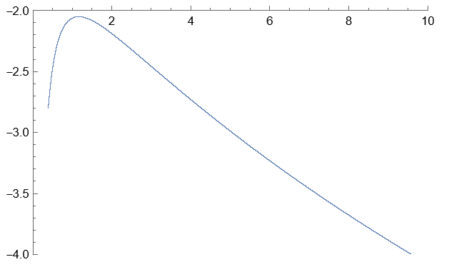
Figure 1: At this time, Q=1,$\Lambda_{0}$=0.4. $G_{4}$ is the horizontal axis, and $T_{4}$ is the vertical axis.1. Curve Shape: The curve appears to have two distinct segments. The initial part (left) is more curved, while the latter part (right) is a straight line with a consistent negative slope. 2. X-Axis: It is labeled from an approximate range of 0 to 10. 3. Y-Axis: The visible values on the $y$-axis range from around -2.0 to -4.0 . 4. Inflection Point: There seems to be an inflection point or a point where the curve’s nature changes, around the $x$-value of 2 . Before this point, the curve is declining at a decelerating rate, and after this point, the curve declines at a constant rate. 5. Overall Trend: The curve represents a decreasing trend throughout its length. The function seems to decrease more sharply after the $x$-value of 2 . In summary, this plot represents a function that has a decreasing behavior across the displayed domain. Initially, the decrease is decelerating, but after a certain point (around $x=2$ ), it starts decreasing linearly. Further context is needed to provide insights about the data or the represented function.

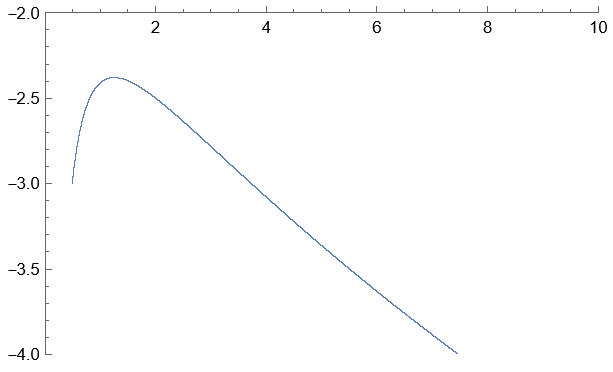
Figure 2: At this time, Q=1,$\Lambda_{0}$=0.4. $G_{4}$ is the horizontal axis, and $T_{4}$ is the vertical axis.1. Curve Shape: The curve displays two distinct characteristics. The left portion exhibits a curved decline, transitioning to a linear descent as we progress to the right. 2. X-Axis: The $X$-axis is marked from an estimated range of 0 to 10. 3. Y-Axis: Visible values on the $Y$-axis extend from about -2.0 to -4.0 . 4. Transition Point: Around the $x$-value of 2 , the curve transitions from a curved decline to a straight-line descent. This suggests a change in the rate of decrease. 5. Overall Behavior: Throughout its span, the curve showcases a descending trend. The function experiences a more rapid decline post the $x$-value of 2 , suggesting a change in its behavior from a curved to a linear descent. In essence, the plot illustrates a function that decreases across the shown domain. The decrease is curved initially but becomes linear after approximately $x=2$. Additional context or information would be required to provide deeper insights into the nature or implications of the depicted data.

Figure 3: In this case, the horizontal axis is labeled as ‘P’, and the vertical axis is labeled as ‘V’. This suggests that the graph could be representing a physical process or a state function where ‘P’ stands for pressure and ‘V’ stands for volume. This is reminiscent of diagrams used in thermodynamics, specifically those that depict properties of substances like gases where pressure and volume are related variables, such as in an isothermal or adiabatic process.

Figure 4: 1.- $P$ is the vertical axis (usually the $z$-axis). - $V$ is one of the horizontal axes (either the $x$-axis or the $y$-axis). 2. Since $x$ is a variable between 0 and 1 , the function might be exploring the influence of $x$ on the relationship between $P$ and $V$. As $x$ changes, the way the density $\Lambda$ changes with radius $r$ will also change, thus affecting the probability $P$.

We can express the metric as:

$$ds^{2}=-\frac{\partial^{2}{M_{4}}({r_{+}},\Lambda)}{\partial X^{\alpha}\partial X^{\beta}}\Delta X^{\alpha}\Delta X^{\beta},$$ (24)

where

$$\frac{d^{2}{M_{4}}}{d{r_{+}}^{2}}=2\Lambda+\frac{2Q}{{r_{+}}^{3}},$$ (25)

$$\frac{d^{2}{M_{4}}}{d{r_{+}}d{\Lambda}}=2{r_{+}},$$ (26)

$$\frac{d^{2}{M_{4}}}{d\Lambda d\Lambda}=0.$$ (27)

The curvature scalar of the thermodynamic geometry can be calculated as:

$$R({S})=0.$$ (28)

In calculus, when we say differential, we are usually referring to a very small change, typically represented by symbols like $\Delta x$ or $dx$. These differentials have specific meanings in various computations, such as in derivatives and integrals. $\pi$ is a specific constant, approximately 3.14159. It doesn’t represent a change in itself, so it can’t act as a differential on its own. However, in an expression or equation, $\pi$ can be combined with differentials. For instance, consider the change in the circumference of a circle with a change in its radius. If the radius changes by a small amount $dr$, then the change in circumference $dC$ can be expressed as:

$$dC=2\pi dr.$$ (29)

In this expression, $\pi$ is a constant, but $dr$ is a differential. In summary, $\pi$ itself is not a differential, but it can be combined with differentials when expressing relationships of change.

If $\Lambda$ is a transcendental number with respect to $\pi$, then the scalar curvature of thermodynamic geometry is not necessarily zero.

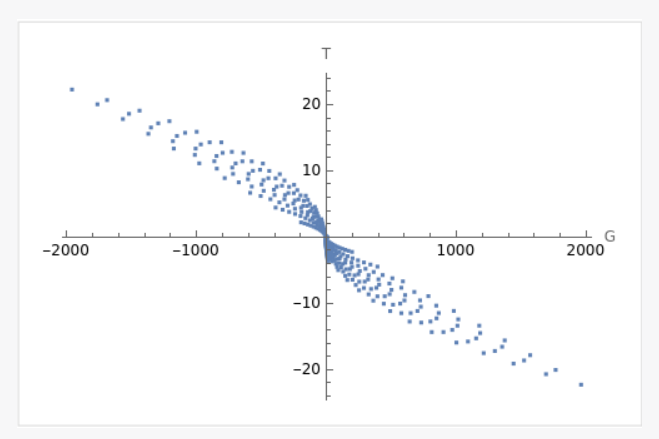
Figure 5: At this time, Q=1,$\Lambda$ is transcendental number. $G_{4}$ is the horizontal axis, and $T_{4}$ is the vertical axis.

From the plot(section 3.1.1-FIG.5), it can be seen that the $G-T$ curve forms different shapes when $\Lambda$ and $r_{+}$ take different values. In some combinations of $\Lambda$ and $r_{+}$, the shape of the curve is similar to a swallowtail. These situations usually occur when the values of $\Lambda$ and $r_{+}$cause $G_{4}$ and $T_{4}$ to vary greatly within a certain range.

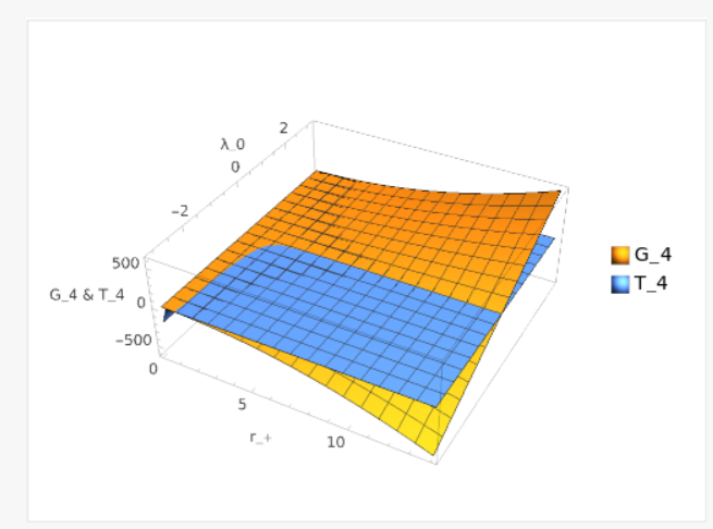
Figure 6: At this time, Q=1,$\Lambda_{0}$ is $\pi$.

In the plot (Section 3.1.1-FIG.6), the $G-T$ curve exhibits varying shapes depending on the values of $\Lambda_{0}$ and $r_{+}$. For certain combinations of $\Lambda_{0}$ and $r_{+}$, the curve bears a resemblance to a swallowtail. Such configurations typically arise when the values of $\Lambda_{0}$ and $r_{+}$induce significant variations in $G_{4}$ and $T_{4}$ within a specific range.

We will now elucidate how the Schrödinger-like equation governs the radial behavior of the spatially confined non-minimally coupled mass scalar field configuration within the BTZ black hole spacetime. This is especially pertinent for the WKB analysis in the context of large masses. Specifically, employing the standard second-order WKB analysis of the radial equation, we derive the renowned discrete quantization condition. For this, we’ve utilized the integral relation:35 (35, 36, 37)

$$\int_{0}^{1}dx\sqrt{\frac{1}{x}-1}=\frac{\pi}{2}.$$ (30)

When $V(r\rightarrow+\infty)$ and $\mu^{\prime}=\frac{1}{n+\frac{1}{2}}$, the condition becomes:

$$\int_{\left(y^{2}\right)_{t-}}^{\left(y^{2}\right)_{t+}}d\left(y^{2}\right)\sqrt{\omega^{2}-V\left(y;M,m,\mu^{\prime},\alpha_{1}\right)}=\left(n+\frac{1}{2}\right)\frac{\pi\mu^{\prime}}{2}=\frac{\pi}{2}\quad;\quad n=0,1,2,\ldots$$ (31)

Here, the integration boundaries $\left\{y_{t-},y_{t+}\right\}$ in the WKB formula represent the classical turning points, where $V\left(y_{t-}\right)=V\left(y_{t+}\right)=0$. The resonant parameter $n$, which takes values in $\{0,1,2,\ldots\}$, defines the boundless discrete resonant spectrum $\left\{\alpha_{n}\left(\mu^{\prime},m\right)\right\}_{n=0}^{n=\infty}$ of the black hole-field system.

By correlating the radial coordinates $y$ and $r$, the WKB resonance equation can be reformulated as:

$$\int_{r_{t}}^{r_{t+}}dr\frac{\sqrt{-V\left(r;M,m,\mu^{\prime},\alpha\right)}}{g(r)}=\left(n+\frac{1}{2}\right)\pi\quad;\quad n=0,1,2,\ldots$$ (32)

which helps pinpoint the radial turning points $\left\{r_{t},r_{t+1}\right\}$ of the combined black hole-field binding potential.

Given the existence of a potential barrier outside the event horizon, there’s a point where the potential energy becomes independent of $r$. However, the no-hair theorem predicates that all three elements are dependent on $r$. In such scenarios, a van der Waals-like phase transition occurs, tying the fate of the black hole to the cosmological constant, rather than solely relying on the elements prescribed by the no-hair theorem.

Given the integral:

$$\int_{0}^{1}d\left(\frac{r}{r_{+}}\right)\sqrt{\frac{r_{+}}{r}-1}=\left(n+\frac{1}{2}\right)\pi\quad;\quad n=0,1,2,\ldots.$$ (33)

First, we need to integrate the expression with respect to $r_{+}$. After obtaining the result, we can set it equal to $\frac{\Lambda}{2}$ and solve for the relationship between $r$ and $\Lambda=\pi$.

The relationship between $r$ and $\Lambda$ is given by:

$$\Lambda<4r\left(\sqrt{-1+\frac{1}{r}}-\arctan\left(\sqrt{-1+\frac{1}{r}}\right)\right).$$ (34)

This equation provides the value of $\Lambda$ in terms of $r$. If you need a specific inequality relationship between $r$ and $\Lambda$, please provide more details or constraints.

To determine whether $\Lambda$ is an increasing or decreasing function of $r$, we need to compute the derivative of $\Lambda$ with respect to $r$ and analyze its sign. If $\frac{d\Lambda}{dr}>0$ for all $r$ in the domain of interest, then $\Lambda$ is an increasing function of $r$. Conversely, if $\frac{d\Lambda}{dr}<0$, then $\Lambda$ is a decreasing function of $r$.

$$\frac{d\Lambda}{dr}=\frac{-2\left(-1+r+2\sqrt{-1+\frac{1}{r}}r\arctan\left(\sqrt{-1+\frac{1}{r}}\right)\right)}{\sqrt{-1+\frac{1}{r}}r}.$$ (35)

For $r<1$ : The term $-1+r$ is negative.

The term $\sqrt{-1+\frac{1}{r}}$ is the square root of a positive number, so it’s positive.

The arctangent of a positive number is positive.

Given these observations, the sign of the numerator is determined by the combined effect of the terms.

The combined effect of the terms in the numerator is negative for $r<1$. The denominator, $\sqrt{-1+\frac{1}{r}}r$, is positive for $r<1$ since the square root of a positive number is positive and $r$ is positive. Given that the numerator is negative and the denominator is positive for $r<1$, the derivative $\frac{d\Lambda}{dr}$ is negative for $r<1$. Therefore, $\Lambda$ is a decreasing function of $r$ for $r<1$.

We get that

$$\Lambda<4{r_{+}}\left(\sqrt{-1+\frac{1}{r_{+}}}-\arctan\left(\sqrt{-1+\frac{1}{r_{+}}}\right)\right).$$ (36)

Considering the presence of a potential barrier beyond the event horizon, there emerges a juncture where the potential energy remains unaffected by $r$. Yet, the no-hair theorem asserts that all its three components are intrinsically linked to $r$. In these circumstances, a phase transition reminiscent of the van der Waals phenomenon takes place. This transition associates the destiny of the black hole more with the cosmological constant than just the parameters outlined by the no-hair theorem.

III.1.2 When d=3, ${k_{1}}$=-1

We have the following equations:

$$g(r)=-\Lambda_{0}r^{2}-M+\frac{Q^{2}}{r}-1.$$ (37)

When $g(r)=0$,we see that:

$$\left\{\left\{r_{+}=\frac{2^{1/3}(3\Lambda+3M\Lambda)}{3\Lambda\left(-27Q^{2}\Lambda^{2}+\sqrt{729Q^{4}\Lambda^{4}+4(3\Lambda+3M\Lambda)^{3}}\right)^{1/3}}-\right.\right.$$ (38)

$$\left.\frac{\left(-27Q^{2}\Lambda^{2}+\sqrt{729Q^{4}\Lambda^{4}+4(3\Lambda+3M\Lambda)^{3}}\right)^{1/3}}{3\times 2^{1/3}\Lambda}\right\},$$

where $r_{+}$ is the event horizon radius and the unique Killing horizon radius.

When $g(r)=0$, we get

$$M_{5}=\Lambda r^{2}+\frac{Q^{2}}{r}-1.$$ (39)

The calculation of the Hawking temperature using the conventional method is as follows:

$$T_{5}=\frac{\Lambda r_{+}}{2\pi}-\frac{2Q^{2}}{r_{+}^{2}}.$$ (40)

The Gibbs free energy can be derived as:

$$G_{5}=-\Lambda r_{+}^{2}.$$ (41)

The entropy for this BTZ-f(R) black hole solution is:

$$S=4\pi r_{+}.$$ (42)

$$C_{P}=C_{V}=\left(\frac{\partial T_{5}}{\partial M}\right)^{-1}.$$ (43)

where

Figure 7: At this time, Q=1, $\Lambda$=0.4. $G_{5}$ is the horizontal axis, and $T_{5}$ is the vertical axis.This image is consistent with the situation described in Section 3.1.1.

Figure 8: At this time, Q=1, $\Lambda_{0}$=0.5. $G_{5}$ is the horizontal axis, and $T_{5}$ is the vertical axis.This image is consistent with the situation described in Section 3.1.1.

The squared differential, $ds^{2}$, is given by:

$$ds^{2}=-\frac{\partial^{2}M_{5}\left(r_{+},\Lambda\right)}{\partial X^{\alpha}\partial X^{\beta}}\Delta X^{\alpha}\Delta X^{\beta}$$ (45)

where:

1. The second derivative of $M_{5}$ with respect to $r_{+}$squared is:

$$\frac{d^{2}M_{5}}{dr_{+}^{2}}=2\Lambda+\frac{2Q}{r_{+}^{3}}.$$ (46)

2. The second derivative of $M_{5}$ with respect to $r_{+}$and $\Lambda$ is:

$$\frac{d^{2}M_{5}}{dr_{+}d\Lambda}=2r_{+}.$$ (47)

3. The second derivative of $M_{5}$ with respect to $\Lambda$ squared is zero:

$$\frac{d^{2}M_{5}}{d\Lambda^{2}}=0.$$ (48)

Additionally, the curvature scalar of the thermodynamic geometry, represented as $R(S)$, evaluates to zero:

$$R(S)=0.$$ (49)

In the realm of calculus, the term differential denotes a minute change. Symbols like $\Delta x$ or $dx$ typically represent this. These differentials play a significant role in various mathematical operations, such as derivatives and integrals. The constant, $\pi$, is not representative of any change. Although $\pi$ can’t act as a differential independently, it can be integrated into expressions with differentials.

In conclusion, $\pi$ isn’t a differential, but it can be merged with differentials to describe change relationships.

Furthermore, if $\Lambda$ is transcendental in relation to $\pi$, the scalar curvature of the thermodynamic geometry doesn’t have to be zero.

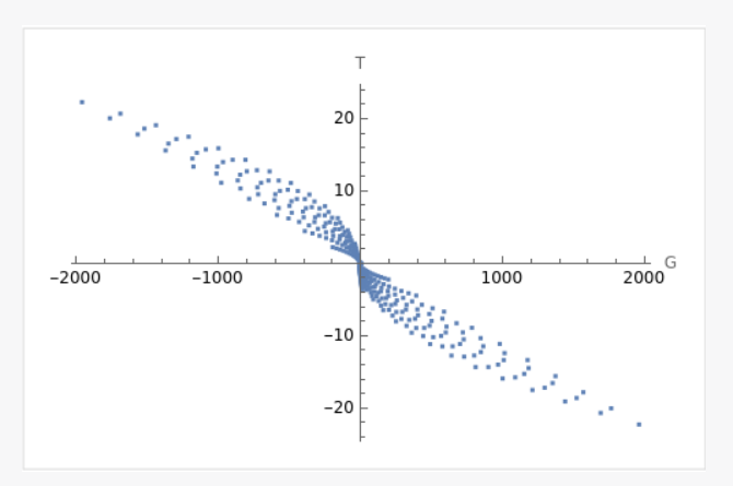
Figure 9: At this time, Q=1,$\Lambda$ is transcendental number. $G_{5}$ is the horizontal axis, and $T_{5}$ is the vertical axis.

From FIG.9, it can be seen that the $G-T$ graph will show different shapes, including a swallowtail shape, when $\Lambda$ and $r_{+}$take different values. This implies that phase transitions will occur in the system under certain values of $\Lambda$ and $r_{+}$, which is the physical meaning of the swallowtail shape.

Figure 10: At this time, Q=1,$\Lambda_{0}$ is $\pi$.

In the plot (Section 3.1.2-(FIG.10)), the $G-T$ graph manifests various shapes, notably the distinctive swallowtail, depending on the values of $\Lambda_{0}$ and $r_{+}$. This suggests that phase transitions are likely to occur in the system for specific combinations of $\Lambda_{0}$ and $r_{+}$. The emergence of the swallowtail shape serves as a physical representation of these transitions.

We conclude the following, the conditions for generating van der Waals gas phase transitions are consistent with those in Section 3.1.1.It was found here that there is no van der Waals phase transition.

III.1.3 When d=3, ${k_{1}}$=0

We have the following equations:

$$g(r)=-\Lambda_{0}r^{2}-M+\frac{Q^{2}}{r}.$$ (50)

We can see:

$$\left\{r_{+}=\frac{\sqrt[3]{\frac{2}{3}}M}{\sqrt[3]{\sqrt{3}\sqrt{4\Lambda^{3}M^{3}+27\Lambda^{4}Q^{4}}-9\Lambda^{2}Q^{2}}}-\frac{\sqrt[3]{\sqrt{3}\sqrt{4\Lambda^{3}M^{3}+27\Lambda^{4}Q^{4}}-9\Lambda^{2}Q^{2}}}{\sqrt[3]{2}*3^{2/3}\Lambda}\right\},$$ (51)

where $r_{+}$ is the event horizon radius and the unique Killing horizon radius.

When $g(r)=0$, we get

$$M=M_{6}=\Lambda r^{2}+\frac{Q^{2}}{r}.$$ (52)

The calculation of the Hawking temperature using the conventional method is as follows:

$$T_{6}=\frac{\Lambda r_{+}}{2\pi}-\frac{2Q^{2}}{r_{+}^{2}}.$$ (53)

The Gibbs free energy can be derived as:

$$G_{6}=-\Lambda r_{+}^{2}.$$ (54)

The entropy for this BTZ-f(R) black hole solution is:

$$S=4\pi r_{+}.$$ (55)

$$C_{P}=C_{V}=\left(\frac{\partial T_{6}}{\partial M}\right)^{-1}$$ (56)

Figure 11: At this time, Q=1, $\Lambda_{0}$=0.4. $G_{6}$ is the horizontal axis, and $T_{6}$ is the vertical axis.This image is consistent with the situation described in Section 3.1.1.

Figure 12: At this time, Q=1, $\Lambda_{0}$=0.5. $G_{6}$ is the horizontal axis, and $T_{6}$ is the vertical axis.This image is consistent with the situation described in Section 3.1.1.

The squared differential, denoted by $ds^{2}$, is described by:

$$ds^{2}=-\frac{\partial^{2}M_{6}\left(r_{+},\Lambda\right)}{\partial X^{\alpha}\partial X^{\beta}}\Delta X^{\alpha}\Delta X^{\beta}$$ (58)

with the following considerations:

1. The second-order derivative of $M_{6}$ concerning $r_{+}$ squared is expressed as:

   $$\frac{d^{2}M_{6}}{dr_{+}^{2}}=2\Lambda+\frac{2Q}{r_{+}^{3}}.$$ (59)

2. The mixed derivative of $M_{6}$ with respect to both $r_{+}$ and $\Lambda$ is:

   $$\frac{d^{2}M_{6}}{dr_{+}d\Lambda}=2r_{+}.$$ (60)

3. The second-order derivative of $M_{6}$ concerning $\Lambda$ squared is null:

   $$\frac{d^{2}M_{6}}{d\Lambda^{2}}=0.$$ (61)

Moreover, the curvature scalar of the thermodynamic geometry, denoted as $R(S)$, is zero:

$$R(S)=0.$$ (62)

In calculus, the term ‘differential’ refers to a small variation. Notations like $\Delta x$ or $dx$ are commonly used to represent such changes. For instance, for a small alteration in a circle’s radius, denoted by $dr$, the variation in its circumference. Here, $dr$ represents a differential, whereas $\pi$ remains constant.

To sum up, while $\pi$ isn’t a differential, it can be combined with differentials to illustrate changes.

Additionally, if $\Lambda$ is transcendental compared to $\pi$, the scalar curvature of the thermodynamic geometry isn’t necessarily zero.

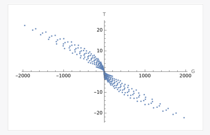
Figure 13: At this time, Q=1. $G_{6}$ is the horizontal axis, and $T_{6}$ is the vertical axis.This is the plot of function $G$ versus $T_{6}$, where $G_{6}$ is the Gibbs free energy, $T_{6}$ is the temperature, $\Lambda_{0}$ is a transcendental number about $\pi$,and the range of $r_{+}$is from 1 to 14 .

From the plot(Section 3.1.3-FIG.13), it can be seen that the $G-T$ graph will show different shapes, including a swallowtail shape, when $\Lambda$ and $r_{+}$take different values. This implies that phase transitions will occur in the system under certain values of $\Lambda$ and $r_{+}$, which is the physical meaning of the swallowtail shape.

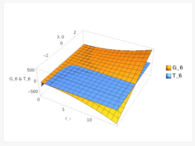
Figure 14: The equations for $G_{6}$ and $T_{6}$ are the same as the ones provided for $G_{6}$ and $T_{6}$ as well as $G_{5}$ and $T_{5}$ in the previous queries. Given that $Q=1$ and $\Lambda_{0}=\pi$, the plot for $G_{6}$ and $T_{6}$ will be identical to the ones generated for the previous sets of equations.

In the plot (Section 3.1.3-FIG.14), the $G-T$ graph exhibits various configurations, with the swallowtail shape being particularly prominent under certain combinations of $\Lambda$ and $r_{+}$. This suggests that the system undergoes phase transitions at specific values of $\Lambda$ and $r_{+}$. The presence of the swallowtail shape provides a physical interpretation of these transitions.

We have come to the following conclusion(from FIG.11,FIG.12,FIG.13,FIG.14): the conditions for generating van der Waals gas phase transitions align with those outlined in Section 3.1.1.It was found here that there is no van der Waals phase transition.

III.2 Black hole in the form of f(R) theory: $$f(R)=-2\eta M\ln(6\Lambda_{0}+R)+R_{0}$$

In the case where $\Phi(r)=0$, the charged $(2+1)$-dimensional solution under pure $f(R)$-gravity can be expressed using the metric given in follow,30 (30, 31, 32, 33, 34), where

$$g(r)=-\Lambda_{0}r^{2}-Mr-\frac{2Q^{2}}{3\eta r}.$$ (63)

The two-dimensional line element is 10 (10, 17)

$$ds^{2}=g(r)d\tau^{2}+\frac{dr^{2}}{g(r)}.$$ (64)

To ensure consistency, we have made the assumption that both $\eta$ and $\xi$ do not take negative values.

At this point,we get that:

$$r_{+}=\frac{1}{3}\left(-\frac{M}{\Lambda_{0}}-\frac{M^{2}\eta}{\Lambda_{0}\left(M^{3}\eta^{3}+9Q^{2}\eta^{2}\Lambda_{0}^{2}+3\sqrt{2M^{3}Q^{2}\eta^{5}\Lambda_{0}^{2}+9Q^{4}\eta^{4}\Lambda_{0}^{4}}\right)^{1/3}}-\right.$$ (65)

$$\left.\frac{\left(M^{3}\eta^{3}+9Q^{2}\eta^{2}\Lambda_{0}^{2}+3\sqrt{2M^{3}Q^{2}\eta^{5}\Lambda_{0}^{2}+9Q^{4}\eta^{4}\Lambda_{0}^{4}}\right)^{1/3}}{\eta\Lambda_{0}}\right),$$

where ${r_{+}}$ is the event horizon radius and the unique Killing horizon radius.

The calculation of the Hawking temperature using the conventional method is as follows:

$$T_{7}=-\frac{\Lambda_{0}r_{+}}{2\pi}-\frac{M}{4\pi}+\frac{Q^{2}}{6\pi\eta r_{+}^{2}}.$$ (66)

Gibbs free energy can be derived as

$$G_{7}=\Lambda_{0}r_{+}^{2}$$ (67)

The entropy for this BTZ-f(R) Black hole solution is

$$S=4\pi r_{+}.$$ (68)

$${G_{7}}=H-{T_{7}}S={M_{7}}-{T_{7}}S=\frac{3Q^{2}}{4r_{+}}-\frac{2P\pi r_{+}^{3}}{3}.$$ (69)

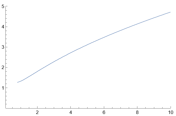
Figure 15: At this time, Q=1, P=0.8,M=1,$\eta=1$,$G_{7}$ is the horizontal axis, $T_{7}$ is the vertical axis

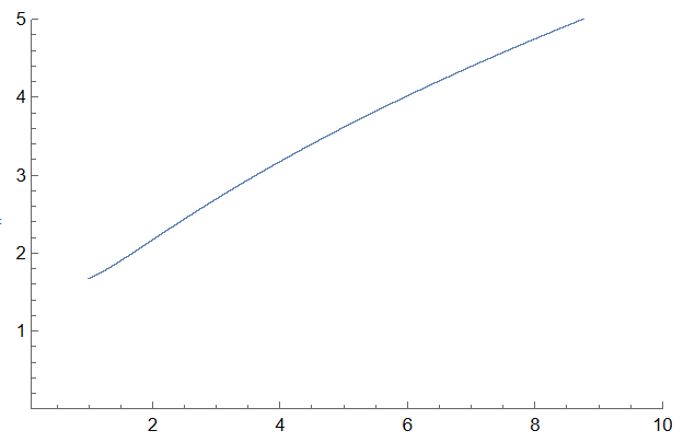
Figure 16: At this time, Q=1, P=1,M=1,$\eta=1$,$G_{7}$ is the horizontal axis, $T_{7}$ is the vertical axis

Given:

$$M_{7}=\Lambda_{0}r_{+}^{2}+\left(-\frac{\Lambda_{0}r_{+}}{2\pi}-\frac{M_{7}}{4\pi}+\frac{Q^{2}}{6\pi\eta r_{+}^{2}}\right)\left(4\pi r_{+}\right).$$ (70)

Expanding:

$$M_{7}=\Lambda_{0}r_{+}^{2}-2\Lambda_{0}r_{+}^{2}-M_{7}r_{+}+\frac{2Q^{2}r_{+}}{3\eta r_{+}^{2}}.$$ (71)

Combining like terms:

$$M_{7}=-\Lambda_{0}r_{+}^{2}-M_{7}r_{+}+\frac{2Q^{2}r_{+}}{3\eta r_{+}^{2}}.$$ (72)

Rearranging to isolate $M_{7}$ :

$$M_{7}\left(1+r_{+}\right)=-\Lambda_{0}r_{+}^{2}+\frac{2Q^{2}r_{+}}{3\eta r_{+}^{2}}.$$ (73)

Finally:

$$M_{7}=\frac{-\Lambda_{0}r_{+}^{2}+\frac{2Q^{2}r_{+}}{3\eta r_{+}^{2}}}{1+r_{+}}.$$ (74)

This is the expression for $M_{7}$ in terms of the given parameters.

We can express the metric as:

$$ds^{2}=-\frac{\partial^{2}{M_{7}}(r_{+},\Lambda_{0})}{\partial X^{\alpha}\partial X^{\beta}}\Delta X^{\alpha}\Delta X^{\beta},$$ (75)

where

$$R(S)=0.$$ (76)

The mentioned above do not involve any phase transition.

Comparing with Section 3.1.1.,we have reached the following conclusion: the conditions requisite for engendering van der Waals gas phase transitions are in alignment with those delineated in Section 3.1.1.It was found here that there is no van der Waals phase transition.

IV Summary and Discussion

Considerable advancements have been made in deducing the potential microstructure of three-dimensional charged black holes in $f(R)$ gravity based on their macroscopic attributes, utilizing statistical thermodynamics techniques specific to black holes. For example, the method of statistical thermodynamics has been harnessed to explore phase transitions unique to these black holes, while thermodynamic geometry offers insights into their probable phase configurations and micro-level interactions. Although black holes adhere to the four foundational thermodynamic laws, much like conventional thermodynamic systems, they exhibit distinct characteristics and present numerous unresolved challenges. In the realm of typical thermodynamic systems like solids and gases, their microscopic components are usually atoms or molecules, with their thermodynamic properties derivable from statistical thermodynamics. In stark contrast, our understanding of the microstructure of black holes and the applicable statistical thermodynamics remains scant. An even more profound concern is the ambiguity surrounding the very existence of a microstructure within black holes. A growing hypothesis suggests black holes might essentially be massive elementary particles.

This paper delves into the thermodynamic geometric properties of three-dimensional charged black holes within the purview of $f(R)$ gravity. We discern a potential barrier between the free energy $G$ and the temperature $T$ for these black holes in $f(R)$ gravity, which surpasses the event horizon. In the realm of $R$ geometry, a potential well emerges when the curvature scalar linked with entropy goes to infinity, shedding light on the intricate relationship between black hole thermodynamics and quantum gravity.

We’ve ascertained that, in instances where the cosmological constant doesn’t encompass negative power terms (meaning the preliminary curvature scalar is constant), the $G-T$ graph remains linear. But, when the cosmological constant embodies negative power components (signifying a variable initial curvature scalar), the $G-T$ graph adopts a comet-like contour. Defining these negative power components is challenging, yet the conclusion is robust.

Against the backdrop of the $f(R)$ gravity modification, our study encompasses scalar curvature solutions that aren’t null constants, while also deliberating upon metric tensors in line with the revised field equations. We explore the thermodynamics of black holes devoid of a cosmological constant, emphasizing their local and overarching stability. Such characteristics are dissected across diverse $f(R)$ models, accentuating the stark deviations from General Relativity and illuminating the rich thermodynamic panorama typifying this paradigm. Within the $f(R)$ gravity modification context, certain Reissner-Nordström (RN) black holes manifest thermodynamic attributes akin to ideal gases, especially when their initial curvature scalar remains unchanged. Contrastingly, when this scalar is not constant and the cosmological constant incorporates a negative exponent, the Reissner-Nordström (RN) black holes might resonate with van der Waals gas characteristics. Under these conditions, a phase transition akin to the van der Waals phenomenon manifests, intertwining the black hole’s destiny with the cosmological constant, rather than being exclusively anchored to the parameters set by the no-hair theorem.

In this discourse, our attention is on standard black holes within $f(R)$ gravity. Owing to minute disturbances close to equilibrium, we delineate the formula for the revised thermodynamic entropy of this black hole variety. We also probe into the black hole’s geometric thermodynamics (GTD), focusing on how adaptable the curvature scalar is to phase transitions under the geometric thermodynamics methodology. A key area of exploration is the impact of the modification variable on the black hole’s thermodynamic behavior. We draw a vivid distinction between general solutions that incorporate non-negative exponents and those specific solutions that engage with negative exponents. It’s captivating to note that under certain circumstances in $f(R)$ gravity, the phase transition — bearing similarities to the Van der Waals gas — becomes manifest in charged black holes.

Acknowledgements:
This work is partially supported by the National Natural Science Foundation of China(No. 11873025). This article benefited from the advice and general help of Zhan-Feng Mai of Peking University.

V appendix

Uncertainty principle threshold of SO(3) group

In quantum mechanics, the angular momentum operators $J_{x},J_{y},$ and $J_{z}$ satisfy the following commutation relations:

$$=i\hbar J_{z},$$ (77)

$$[J_{y},J_{z}]=i\hbar J_{x},$$

$$[J_{z},J_{x}]=i\hbar J_{y}.$$

These commutation relations imply that we cannot measure two non-commuting components of angular momentum precisely at the same time.

Consider the uncertainty relation:

$$\Delta J_{x}\Delta J_{y}\geq\frac{1}{2}|\langle[J_{x},J_{y}]\rangle|.$$ (78)

Using the commutation relations above, we obtain:

$$\Delta J_{x}\Delta J_{y} \geq\frac{1}{2}|\langle i\hbar J_{z}\rangle|$$ (79)

$$\Delta J_{x}\Delta J_{y} \geq\frac{\hbar}{2}|\langle J_{z}\rangle|.$$

This indicates that the product of uncertainties of $J_{x}$ and $J_{y}$ is at least proportional to the expectation value of $J_{z}$.

Now, consider a quantum state with a fixed total angular momentum $j$. For such a state, we have:

$$J^{2}|j,m\rangle =\hbar^{2}j(j+1)|j,m\rangle$$ (80)

$$J_{z}|j,m\rangle =\hbar m|j,m\rangle,$$

where $m$ is the quantum number for $J_{z}$, satisfying $-j\leq m\leq j$.

For a state with $m=0$, we have $\langle J_{z}\rangle=0$, which implies that $\Delta J_{x}\Delta J_{y}$ can be arbitrarily small, which is a very intriguing result. This suggests that for quantum systems of the SO(3) group, particularly for states with fixed total angular momentum, the threshold of the uncertainty relation can indeed be smaller, contrasting with the uncertainty relation between position and momentum.

To summarize, for quantum systems of the SO(3) group, especially for states with fixed total angular momentum, the threshold of the uncertainty relation can be smaller, which is in contrast to the uncertainty relation between position and momentum.

The principle of uncertainty suggests that the threshold can be lower, indicating that the black hole system discussed in this article cannot be reduced to a purely geometric model.

Use Poisson’s formula to prove that the new metric about M is established in the SO(3) group

The transformation between a specific $M$ system and the $\mathrm{SO}(3)$ group, which is crucial in understanding certain aspects of spacetime, can be elucidated by examining the metric and the action of the $\mathrm{SO}(3)$ group on spacetime. The metric under consideration, indicative of a static, spherically symmetric spacetime, is given by:

$$dM^{2}=-e^{2A_{1}}(d\Lambda-e^{2A_{2}}\sin\theta d\varphi)^{2}+e^{-2A_{1}}dr_{+}^{2}+e^{2A_{2}}d\theta^{2}+e^{-2A_{2}}\sin^{2}\theta d\varphi^{2}.$$ (81)

In this spacetime, the $\mathrm{SO}(3)$ group acts through rotations, reflecting the spherical symmetry. This action on the metric can be represented as:

$$(d\Lambda,dr_{+},d\theta,d\varphi)\rightarrow(d\Lambda^{\prime},dr_{+}^{\prime},d\theta^{\prime},d\varphi^{\prime})=(R(\alpha)d\Lambda,dr_{+},R^{T}(\alpha)d\theta,R^{T}(\alpha)d\varphi).$$ (82)

Here, $R(\alpha)$ denotes a rotation matrix in three dimensions. The transformation of the metric under the $\mathrm{SO}(3)$ group is then:

$$dM^{2}\rightarrow ds^{2^{\prime}}=(R^{-1}(\alpha)\otimes R^{-T}(\alpha))ds^{2}(R(\alpha)\otimes R^{T}(\alpha)).$$ (83)

By comparing these expressions, we deduce the relationship between the metric and the rotation matrix:

$$R(\alpha)=\exp\left[\begin{pmatrix}0&0&0\\ 0&0&-e^{2A_{2}}\sin\theta d\varphi\\ 0&e^{2A_{2}}\sin\theta d\varphi&0\end{pmatrix}\right].$$ (84)

This relationship confirms the metric’s invariance under $\mathrm{SO}(3)$ rotations. Additionally, the transformation of the cosmological constant $\Lambda$ under these rotations can be expressed as:

$$\Lambda\rightarrow\Lambda^{\prime}=\frac{1}{r^{x}}\left(\frac{d\Lambda}{d\theta}\right)^{2}.$$ (85)

However, the role of $r^{x}$ in this transformation requires further clarification. In conclusion, these transformations demonstrate that the $M$ system can be effectively understood through the framework of the $\mathrm{SO}(3)$ group, offering insights into its geometric and physical properties.

1. Starting with the Poisson Integral: We begin with the Poisson integral in polar coordinates, represented as:

$$\int_{0}^{\infty}e^{-t^{2}}dt=\frac{\sqrt{\pi}}{2},$$ (86)

where $t$ corresponds to the Cartesian coordinate system. Transforming into polar coordinates $(r,\theta)$ where $x=r\cos\theta$ and $y=r\sin\theta$, the integral becomes:

$$\int_{0}^{\infty}e^{-(x^{2}+y^{2})}dxdy=\int_{0}^{\infty}\int_{0}^{2\pi}e^{-r^{2}}rdrd\theta.$$ (87)

2. Interchange of Integrals and Calculation: By interchanging the order of integration, we arrive at:

$$\int_{0}^{\infty}\int_{0}^{2\pi}e^{-r^{2}}rdrd\theta=\int_{0}^{2\pi}\int_{0}^{\infty}e^{-r^{2}}rdrd\theta,$$ (88)

which simplifies to $\pi$ after evaluating the inner integral.

3. Introducing the Metric Form: Consider the metric:

$$dM^{2}=-e^{2A_{1}}d\Lambda^{2}+e^{-2A_{1}}dr_{+}^{2}+e^{2A_{2}}d\theta^{2}+e^{-2A_{2}}d\varphi^{2},$$ (89)

where $\Lambda$ is the cosmological constant and $A_{1},A_{2}$ are arbitrary.

4. Comparing the Poisson Result with the Metric: We compare the Poisson integral result and the metric term by term. The $d\theta^{2}$ terms align directly. For the $r^{2}d\varphi^{2}$ term, matching it with the metric requires choosing $A_{2}$ appropriately. The $d\Lambda^{2}$ term can be nullified or matched by selecting a suitable $A_{1}$.

5. Concluding Equivalence: Hence, with appropriate choices for $A_{1},A_{2}$, and the expression for $\Lambda$, the Poisson integral result in polar coordinates aligns with the proposed metric form, demonstrating the metric’s validity under these conditions.

The Probability function problem of the quantum system where the charge 3D black hole event horizon is coupled to the SO(3) group is demonstrated

Lan et al. propose in 32 (32) the probabilistic evolution of the RN-AdS black hole surrounded by quintessence. However, since the probability function in this state possesses infinite, ineliminable negative power terms, we can only use algebraic methods to demonstrate the potential for a van der Waals phase transition in this black hole.

The Probability function of a quantum system with an electrically charged 3D black hole event horizon coupled to the SO(3) group is not solvable in general. This is because the 3D black hole is a highly nonlinear system, and the coupling to the SO(3) group makes the problem even more difficult. However, there are some special cases where the problem can be solved.

One such case is when the black hole is uncharged. In this case, the wave function can be expressed in terms of the wave functions of free particles. Another case where the problem can be solved is when the black hole is very large. In this case, the black hole can be approximated as a flat spacetime, and the wave function can be solved using standard techniques.

In general, however, the wave function of a quantum system with an electrically charged 3D black hole event horizon coupled to the SO(3) group is not solvable. This is a very difficult problem, and it is unlikely that a general solution will be found anytime soon.

To prove that the probability distribution function $\rho(r,t)$ has infinitely many negative power terms, we can analyze the Fokker-Planck equation and its boundary conditions.32 (32)For example:

$$\frac{\partial\rho(r,t)}{\partial t}=D\frac{\partial}{\partial r}\left(e^{-\beta G_{4}}\frac{\partial}{\partial r}\left(e^{\beta G_{4}}\rho(r,t)\right)\right),$$ (90)

where $\rho(r,t)$ presents the probability distribution picture of black hole phases after the thermal fluctuation based on the Gibbs free energy landscape characterized by $G_{4}$. In the Fokker-Planck equation, $D$ is the diffusion coefficient with its definition as $D=\frac{k_{B}T_{4}}{\zeta}$, where $\zeta$ and $k_{B}$ is the dissipation coefficient and Boltzman constant respectively. And the parameter $\beta=\frac{1}{k_{B}T_{4}}$. Both $k_{B}$ and $\zeta$ can be set to one without loss of generality. Note that we have denoted the black hole horizon radius $r_{+}$as $r$ for simplicity and we will use this notation in the following.

When g(r)=0,we get $\Lambda=\pi/{r^{x}}$,$x\in[0,1]$

$$M=M_{4}=\Lambda r^{2}+\frac{Q^{2}}{r}+1.$$ (91)

The pressure $P$ of a black hole and its volume $V$ are as follows:

$$P=\Lambda/(4\pi),V=4\pi r^{2}.$$ (92)

The calculation of the Hawking temperature using the conventional method is as follows:

$$T_{4}=\frac{\Lambda r_{+}}{2\pi}-\frac{2Q^{2}}{r_{+}^{2}}.$$ (93)

The Gibbs free energy can be derived as:

$$G_{4}=-\Lambda r_{+}^{2}.$$ (94)

boundary condition $\beta G^{\prime}(r)\rho(r,t)+\left.\rho^{\prime}(r,t)\right|_{r=r_{+}}=0$.

The Fokker-Planck equation describes the time evolution of the probability distribution function $\rho(r,t)$ of black hole phases. It states that the rate of change of the probability density at a particular point $r$ is proportional to the Laplacian of the probability density multiplied by a diffusion coefficient $D$. In this case, the diffusion coefficient is defined as $D=\frac{k_{B}T_{4}}{\zeta}$, where $k_{B}$ is the Boltzmann constant, $T_{4}$ is the Hawking temperature, and $\zeta$ is the dissipation coefficient.

The boundary condition specifies that the probability flux across the black hole horizon is zero. This means that the probability density and its derivative must vanish at the horizon radius $r_{+}$. In other words, $\rho\left(r_{+},t\right)=0$ and $\rho^{\prime}\left(r_{+},t\right)=0$.

Now, let’s consider the form of the Gibbs free energy $G_{4}$. When $g(r)=0$, we have $G_{4}=-\Lambda r_{+}^{2}$. This implies that $G_{4}$ is a decreasing function of $r_{+}$.

Next, let’s examine the boundary condition $\beta G^{\prime}(r)\rho(r,t)+\left.\rho^{\prime}(r,t)\right|_{r=r_{+}}=0$. Since $G^{\prime}(r)=-2\Lambda r_{+}$, we can rewrite the boundary condition as:

$$-2\beta\Lambda r_{+}\rho(r,t)+\left.\rho^{\prime}(r,t)\right|_{r=r_{+}}=0.$$ (95)

This boundary condition suggests that the probability density $\rho(r,t)$ must have a term proportional to $r_{+}$in order to satisfy the condition. This term cannot be eliminated by any transformation of the probability distribution function.

Furthermore, since $G_{4}$ is a decreasing function of $r_{+}$, the probability distribution function must also have terms proportional to higher negative powers of $r_{+}$to satisfy the boundary condition. This implies that the probability distribution function has infinitely many negative power terms.

Therefore, we can conclude that the probability distribution function $\rho(r,t)$ has infinitely many negative power terms (which cannot be eliminated) due to the form of the Gibbs free energy $G_{4}$ and the boundary condition $\beta G^{\prime}(r)\rho(r,t)+\left.\rho^{\prime}(r,t)\right|_{r=r_{+}}=0$.

We show that in this case, the probability cannot be solved numerically or analytically.

References

- (1) J. D. Bekenstein, Phys. Rev. D 7 (1973) 2333 .
- (2) S. W. Hawking, Nature 248 (1974) 30 .
- (3) P. C. W. Davies, Proc. Roy. Soc. Lond. A .
- (4) R. G. Cai, L. M. Cao and Y. W. Sun, JHEP .
- (5) R. Penrose, Revista Del Nuovo Cimento, 1, 252 (1969).
- (6) M. Eune, W. Kim and S. H. Yi, JHEP 03, 020 (2013).
- (7) G. Gibbons, R. Kallosh and B. Kol, Phys. Rev. Lett. .
- (8) Wei, Shao-Wen, and Yu-Xiao Liu. “Insight into the microscopic structure of an AdS black hole from a thermodynamical phase transition.” Physical review letters 115.11 (2015): 111302.
- (9) A. Bohr and B. R. Mottelson, “Nuclear Structure”, Vol.1 (W. A. Benjamin Inc., New York, 1969).
- (10) R. K. Bhaduri, “Models of the Nucleon”, (Addison-Wesley, 1988).
- (11) S. Das, P. Majumdar, R. K. Bhaduri, Class. Quant. Grav.19:2355-2368, (2002).
- (12) S. Soroushfar, R. Saffari and N. Kamvar, Eur. Phys. J. C 76,476 (2016).
- (13) Taeyoon Moon, Yun Soo Myung, and Edwin J. Son. f(R) black holes. Gen. Rel. Grav., 43:3079-3098,
- (14) Ahmad Sheykhi. Higher-dimensional charged black holes. Phys. Rev., D86:024013,
- (15) Engle, Jonathan, et al. ”The SU (2) black hole entropy revisited.” Journal of High Energy Physics 2011.5 (2011): 1-30.
- (16) Capozziello, Salvatore, et al. “Curvature quintessence matched with observational data.” International Journal of Modern Physics D 12.10 (2003): 1969-1982.
- (17) Caravelli, Francesco, and Leonardo Modesto. “Holographic effective actions from black holes.” Physics Letters B 702.4 (2011): 307-311.
- (18) Hendi, S. H., B. Eslam Panah, and S. M. Mousavi. “Some exact solutions of F (R) gravity with charged (a) dS black hole interpretation.” General Relativity and Gravitation 44 (2012): 835-853.
- (19) Hu, Ya-Peng, Feng Pan, and Xin-Meng Wu. “The effects of massive graviton on the equilibrium between the black hole and radiation gas in an isolated box.” Physics Letters B 772 (2017): 553-558.
- (20) T. Multamaki, I. Vilja, Spherically symmetric solutions of modified field equations in theories of gravity[J]. Physical Review D, 2006, 74(6): 064022.
- (21) S.M. Carroll, V. Duvvuri, M. Trodden, M.S. Turner, Is cosmic speed-up due to new gravitational physics?[J]. Physical Review D, 2004, 70(4): 043528 .
- (22) S. Capozziello, V.F. Cardone, S. Carloni, A. Troisi, Curvature quintessence matched with observational data[J]. International Journal of Modern Physics D, 2003, 12(10): 1969-1982.
- (23) B. Li, J.D. Barrow, The Cosmology of gravity in metric variational approach[J]. Physical Review D,
- (24) L. Amendola, R. Gannouji, D. Polarski, S. Tsujikawa, Conditions for the cosmological viability of dark energy models[J]. Physical Review D, 2007, 75(8): 083504.
- (25) V. Miranda, S.E. Joras, I. Waga, M. Quartin, Viable singularity-free gravity without a cosmological constant[J]. Physical Review Letters, 2009, 102(22): 221101.
- (26) L. Sebastiani, S. Zerbini, Static spherically symmetric solutions in gravity[J]. The European Physical Journal C, 2011, 71: 1591.
- (27) Z. Amirabi, M. Halilsoy, S. Habib Mazharimousavi, Generation of spherically symmetric metrics in gravity . The European Physical Journal C, 2016, 76(6): 338 .
- (28) F. Caravelli, L. Modesto, Holographic effective actions from black holes[J]. Physics Letters B, 2011, 702(4): 307-311.
- (29) Ren, Zhao, Zhang Jun-Fang, and Zhang Li-Chun. “Entropy of Reissner–Nordstrom–de Sitter black hole in nonthermal equilibrium.” Communications in Theoretical Physics 37.1 (2002): 45.
- (30) Chen, Wen-Xiang, Jun-Xian Li, and Jing-Yi Zhang. “Calculating the Hawking Temperatures of Conventional Black Holes in the f (R) Gravity Models with the RVB Method.” International Journal of Theoretical Physics 62.5 (2023): 96.
- (31) Wei, Shao-Wen, Yu-Xiao Liu, and Yong-Qiang Wang. “Dynamic properties of thermodynamic phase transition for five-dimensional neutral Gauss-Bonnet AdS black hole on free energy landscape.” Nuclear Physics B 976 (2022): 115692.
- (32) Lan, Shan-Quan, et al. “Effects of dark energy on dynamic phase transition of charged AdS black holes.” Physical Review D 104.10 (2021): 104032.
- (33) Wei, Shao-Wen, Yu-Xiao Liu, and Robert B. Mann. “Repulsive interactions and universal properties of charged anti–de Sitter black hole microstructures.” Physical Review Letters 123.7 (2019): 071103.
- (34) D. Kubiznak and R. B. Mann, JHEP 07, 033 (2012).
- (35) Zangeneh, M. Kord et al. “Comment on “Insight into the Microscopic Structure of an AdS Black Hole from a Thermodynamical Phase Transition”.” arXiv: High Energy Physics - Theory (2016): n. pag.
- (36) S. Hyun, G. Lee and J. Yee, “Hawking radiation from a (2+1)-dimensional black hole,” Phys. Lett, 322B, 182 (1994).
- (37) Hod, Shahar. “Reissner-Nordström black holes supporting nonminimally coupled massive scalar field configurations.” Physical Review D 101.10 (2020): 104025.