PhenomXO4a: a phenomenological gravitational-wave model for precessing black-hole binaries
with higher multipoles and asymmetries

Abstract

In this work we introduce PhenomXO4a, the first phenomenological, frequency-domain gravitational waveform model to incorporate multipole asymmetries and precession angles tuned to numerical relativity. We build upon the modeling work that produced the PhenomPNR model and incorporate our additions into the IMRPhenomX framework, retuning the coprecessing frame model and extending the tuned precession angles to higher signal multipoles. We also include, for the first time in frequency-domain models, a recent model for spin-precession-induced multipolar asymmetry in the coprecessing frame to the dominant gravitational-wave multipoles. The accuracy of the full model and its constituent components is assessed through comparison to numerical relativity and numerical relativity surrogate waveforms by computing mismatches and performing parameter estimation studies. We show that, for the dominant signal multipole, we retain the modeling improvements seen in the PhenomPNR model. We find that the relative accuracy of current full IMR models varies depending on location in parameter space and the comparison metric, and on average they are of comparable accuracy. However, we find that variations in the pointwise accuracy do not necessarily translate into large biases in the parameter estimation recoveries.

I Introduction

The properties of compact-binary gravitational-wave (GW) sources are inferred by convolving detector data with theoretical signal models Abbott et al. (2018); Aasi et al. (2015); Acernese et al. (2015); Akutsu et al. (2021); Abbott et al. (2019, 2021a, 2021b, 2023a); Nitz et al. (2023); Venumadhav et al. (2020); Mehta et al. (2023). In LIGO-Virgo-KAGRA (LVK) compact binary observations to date the most commonly used families of signal models have been Phenom, SEOBNR and NRSurrogate Husa et al. (2016); Khan et al. (2016); Hannam et al. (2014); London et al. (2018); Dietrich et al. (2019); Khan et al. (2020); Thompson et al. (2020); Pratten et al. (2020); García-Quirós et al. (2020); Pratten et al. (2021); Estellés et al. (2022); Taracchini et al. (2014); Pan et al. (2014); Cotesta et al. (2018); Ossokine et al. (2020); Matas et al. (2020); Pompili et al. (2023); Ramos-Buades et al. (2023); Blackman et al. (2017); Varma et al. (2019a, b); Islam et al. (2021a) The Phenom and SEOBNR models are constructed from a combination of analytic or semianalytic approximations during the inspiral, and numerical relativity (NR) calculations for the late inspiral, merger and ringdown; the NRSurrogate models are constructed primarily from NR waveforms. The accuracy of Phenom and SEOBNR models is determined by the accuracy of the analytic ingredients, by the length, accuracy and parameter-space coverage of the NR waveforms, and by the details of the model construction, including any physical approximations. By contrast, the main limitation in current surrogate models is not their accuracy, but their parameter-space coverage and the length of the input waveforms (which, given the fixed frequency range of detector sensitivities, limits the masses at which they can be used for analysis).

Two of the limitations in the Phenom and SEOBNR models used in the first three LVK observing runs (O1-3) were that precession effects (due to spins misaligned with the orbital angular momentum) are based only on analytic approximations and do not include tuning to any NR simulations of precessing binaries, and that the models neglect an asymmetry in the multipoles that is present in precessing configurations. In this paper we present a new model that adds both of these features, PhenomXO4a (XO4a). (Throughout the paper we will introduce each model with its full name, but also introduce an abbreviation, which we we will use to simplify reference throughout the paper to a large number of models with very similar names.)

This paper extends on the work in Ref. Hamilton et al. (2021) (Paper I ​​), and we refer the reader to this paper for more background on the phenomenology of precessing binaries, and a summary of approaches to modelling the GW signal from them. Paper I presented the PhenomPNR (PNR) model, where merger-ringdown precession effects in the $\ell=2$ multipoles were tuned to 40 NR simulations of single-spin systems between mass ratios of $1\leq q=m_{1}/m_{2}\leq 8$, where $m_{1}$ and $m_{2}$ are the component masses of the binary system with $m_{1}\geq m_{2}$, and the primary black hole has dimensionless spin $\chi$ misaligned from the orbital angular momentum by $\theta_{\rm LS}$.

In this work the model is retuned to all 80 simulations in the NR catalogue discussed in Ref. Hamilton et al. (2023a), to improve the overall accuracy of the phenomenological fits, but in particular the behavior of low-spin binaries near the aligned-spin limit. The resulting model is implemented within the IMRPhenomX infrastructure Pratten et al. (2021). We also extend the model of the precession dynamics to higher multipoles through an approximate frequency mapping analogous to that used to construct higher signal multipoles in the earlier PhenomHM model London et al. (2018), and make use of an estimate of the ringdown frequency for each multipole in a frame that tracks the binary’s precession, as presented in Ref. Hamilton et al. (2023b).

We incorporate a model for the multipole asymmetry in the dominant $(\ell,|m|)=(2,2)$ multipoles based on a prescription presented in Ref. Ghosh et al. (2023). This allows us to easily construct the antisymmetric contribution to the dominant multipole from physical quantities that were already modeled for the symmetric contribution, namely the signal amplitude, phase, and one of the three Euler angles that specify the precession.

The current model is the first frequency-domain higher-multipole inspiral-merger-ringdown model to include precession tuning to NR and multipole asymmetry, and provides a first indication of the accuracy improvements each new feature provides, and improvements that need to be made in future to meet the accuracy needs of gravitational-wave observatories.

One issue that arises in frequency-domain models is with the now-standard procedure to separately model (a) the signal in a coprecessing frame that tracks the precession, and (b) the time- or frequency-dependent rotation transformation between the inertial and co-precessing frames. These two models are then combined to produce the final inertial-frame model. This approach is motivated by the observation that the signal multipoles take a simpler form in the co-precessing frame Schmidt et al. (2012), and is used in some form in all precessing Phenom, SEOBNR and NRSurrogate models.

In the time domain the co-precessing frame defined with respect to the $\ell=2$ multipoles is approximately the same as that defined with respect to all multipoles, i.e., the directions that maximise the power emitted by either the $\ell=2$ multipoles or all multipoles are approximately the same. This is not the case in the frequency domain. This is easiest to see when considering the ringdown. The ringdown frequency of the $(\ell,|m|)=(4,4)$ multipole is roughly twice that of the $(\ell,|m|)=(2,2)$ multipole, and so in the frequency domain the $(4,4)$ ringdown will begin at a frequency where there is no longer any power remaining in the $(2,2)$. By contrast, in the time domain the ringdown begins at roughly the same time for all multipoles. We discuss this issue further in Sec. II, and the approximations we use to circumvent the issue in the current model.

A number of earlier models are referred to throughout this paper. For ease of reference we summarize them here. We start with Phenom models. The aligned-spin Phenom model PhenomD Husa et al. (2016); Khan et al. (2016) includes only the dominant multipoles, and was tuned to simulations of (predominantly) single-spin or equal-spin binaries, up to mass ratios of $q=18$. This was used as the basis of the coprecessing-frame model for the precessing-binary models PhenomPv2 Hannam et al. (2014) and PhenomPv3 Khan et al. (2019); NR calibration to in-plane-spin modifications are added to produce PhenomDCP (DCP), which is the co-precessing-frame model for the NR-tuned precession model PNR Hamilton et al. (2021). The more recent aligned-spin models for the dominant multipoles (IMRPhenomXAS (XAS) Pratten et al. (2020)) and higher multipoles (IMRPhenomXHM García-Quirós et al. (2020)) are tuned to NR simulations of unequal-spin binaries, and this is the basis of the coprecessing-frame model for the precessing model IMRPhenomXPHM (XPHM) Pratten et al. (2021). In this work we incorporate NR in-plane-spin tuning to produce IMRPhenomXHM-CP (XHM-CP).

The precession dynamics are modeled in PhenomPv3 using a multi-scale analysis (MSA) approach Chatziioannou et al. (2017), and these are also adopted in XPHM. The MSA dynamics are augmented by NR-tuned merger-ringdown modeling in PNR, which we extend in this work. Alternatively, one may use a frequency-domain parameterization of the time-domain spin evolution used in the time-domain Phenom model IMRPhenomTPHM (TPHM) Estellés et al. (2022); these angles are used in the XPHM-ST model Colleoni et al. (2024), and an efficient method for solving and implementing them is found in IMRPhenomXODE Yu et al. (2023).

The SEOBNR models integrate the EOB equations of motion (with additional NR tuning) to calculate both the inspiral phasing and precession dynamics, followed by smoothly connecting ringdown modes at merger. These models are tuned only to aligned-spin NR waveforms, although precessing-binary waveforms are used for verification of the final model. In this paper we compare against the most recent SEOBNR model, SEOBNRv5PHM (SEOBv5) Ramos-Buades et al. (2023).

Finally, the NRSurrogate model NRSur7dq4 (NRSur) Varma et al. (2019b) is calibrated to precessing NR waveforms up to $q=4$, and can be used to analyze signals starting around $20$ Hz with masses $M\gtrsim 65\,M_{\odot}$. Comparisons against NR waveforms suggest that this is the most accurate model currently available, and we use it for comparisons where possible. However, since it cannot be used for low-mass signals, and its calibration region does not extend beyond $q=4$ (we calibrate our model up to $q=8$), it cannot provide a definitive test of our model across the full calibration parameter space. (Conversely, the lack of an extremely accurate full inspiral-merger-ringdown model across the full binary parameter space is the primary motivation for the work we present here.)

Sec. III outlines how the original DCP tuning is improved and applied to XAS Pratten et al. (2020), as well as introduces the model for the antisymmetric contributions added to the coprecessing $(\ell,|m|)=(2,2)$ multipoles. Information about the precession angles, including modifications to the PNR angles and the mapping of these angles to higher multipoles is found in Sec. IV. The performance of the final model is considered in Sec. V, presenting mismatch and parameter estimation results compared with other contemporary waveform approximants, and we end with concluding remarks in Sec. VI.

In this paper we use geometric units, whereby $G=c=1$. Unless otherwise stated, all frequencies are presented in dimensionless units $Mf$. We employ use of the symmetric mass-ratio $\eta=m_{1}m_{2}/(m_{1}+m_{2})^{2}$, the effective aligned-spin parameter $\chi_{\text{eff}}$ Ajith et al. (2011); Santamaria et al. (2010) and the precession spin parameter $\chi_{\text{p}}$ Schmidt et al. (2015). Finally we remark that results in this paper were produced using the reviewed implementation of this model in LALSuite LIGO Scientific Collaboration (2018); Wette (2020), where the model is called IMRPhenomXO4a.

II On the importance of frame choices

Precession introduces modulations in the amplitude and phase of a gravitational-wave signal, and this complicates both the signal and, as a result, the task of modeling it. One common modeling technique is to make a time-dependent rotation to a “coprecessing” frame that tracks the orbital precession. In such a frame the constituent parts of the signal — the coprecessing-frame waveform and the time-dependent rotation angles (with respect to the total angular momentum, $\mathbf{J}$) — take on simple forms that make them easier to model. In addition, during the inspiral the coprecessing-frame signal can be approximated well by the signal from an equivalent non-precessing binary Schmidt et al. (2012). This is possible because, to a good approximation, the orbital frequency and inspiral rate are determined by the black-hole masses and the spin components that are aligned with the orbital angular momentum, i.e., the spins that constitute an aligned-spin system, and this orbital motion is the dominant contribution to the GW signal; the precession due to the in-plane spin components can be considered as a time-dependent rotation applied to this aligned-spin waveform.

This simplification, which is easy to motivate in the quadrupole approximation to the signal from an orbiting binary, also extends to the sub-dominant multipoles Schmidt et al. (2011), and, although the aligned-spin mapping is no longer valid through merger and ringdown Schmidt et al. (2012); Pekowsky et al. (2013); Ramos-Buades et al. (2020), the coprecessing-frame waveform and the time-dependent precession angles retain a sufficiently simple morphology that the coprecessing frame continues to be attractive for signal modeling.

Some form of coprecessing-frame decomposition has been used in all precessing-binary models that have been used to analyze LVK observations to date Hannam et al. (2014); Khan et al. (2020); Pratten et al. (2021); Estellés et al. (2022); Hamilton et al. (2021); Taracchini et al. (2014); Pan et al. (2014); Ossokine et al. (2020); Ramos-Buades et al. (2023); Varma et al. (2019b). The coprecessing frame can be defined either using the orbital dynamics of the binary, or a frame aligned with the maximum strength of the gravitational-wave signal, referred to as either quadrupole alignment Schmidt et al. (2011) or the optimal emission direction O’Shaughnessy et al. (2011); Boyle et al. (2011). The SEOBNR Pan et al. (2014); Taracchini et al. (2014); Ossokine et al. (2020) and Phenom Hannam et al. (2014); Khan et al. (2020); Pratten et al. (2021); Estellés et al. (2022); Yu et al. (2023) models used the precession defined via the orbital dynamics, while the more recent PNR model Hamilton et al. (2021), and the NRSurrogate models Blackman et al. (2017); Varma et al. (2019b) use the optimal emission direction, which is the correct transformation between the coprecessing frame and the inertial frame of the gravitational wave signal; the differences between coprecessing frames defined with respect to either the signal or the dynamics, are discussed further in
Paper I ​.

Unfortunately, the approximate mapping between precessing- and aligned-spin-binary waveforms does not carry over to the frequency domain beyond the dominant coprecessing-frame multipoles, $(\ell,|m|)=(2,2)$: the optimal emission direction no longer identifies a frame in which the signal multipoles can be approximated by their aligned-spin counterparts.

To illustrate this, first consider the early inspiral in a coprecessing frame in the time domain. We make use of the standard decomposition of the gravitational wave strain, $h(t)$, into spin-weighted spherical harmonics,

$$h(t)=\sum_{\ell,m}h_{\ell,m}(t)\,^{-2}Y_{\ell,m}(\theta,\phi),$$ (1)

where $(\theta,\phi)$ are the standard polar and azimuthal angles in spherical polar coordinates, and $\ell\geq 2$ and $|m|\leq\ell$. As already noted, in this coprecessing frame the signal multipoles will approximate those of an aligned-spin, non-precessing binary, i.e.,

$$h^{\rm{NP}}_{\ell m}(t)=A_{\ell m}(t)e^{-im\Phi(t)},$$ (2)

where $\Phi(t)$ is the orbital phase of the binary and $A_{\ell m}(t)$ the amplitude. At each time $t$, we can rotate the multipoles using a set of Euler angles $\left(\alpha(t),\beta(t),\gamma(t)\right)$ to produce the multipoles in the inertial frame.

Now consider the same early inspiral signal in the frequency domain. We see from Eq. (2) that the frequency of each multipole scales with $m$. If at time $t_{0}$ the frequency of the dominant $(\ell,|m|)=(2,2)$ multipole is $f_{0}$, then the frequency of each other multipole is $mf_{0}/2$. This means that the angles $(\alpha(t),\beta(t),\gamma(t))$ should be applied to the (2,2) multipoles at $f_{0}$, but to the (3,3) multipoles at $3f_{0}/2$, the (4,4) multipoles at $2f_{0}$, and so on. Conversely, if we now consider the signal at only one frequency, $f_{0}$, then the angles $(\alpha,\beta,\gamma)$ applicable to rotate back to the inertial frame will be different for each $m$. (This is what is currently done in the stationary phase approximation [SPA] treatment of the twisting-up procedure in the PhenomPv3HM and XPHM models Pratten et al. (2021); Khan et al. (2020).)

Therefore, we cannot rotate between the coprecessing frame as defined above and the inertial frame at each frequency by a single set of Euler angles. Since the optimal emission direction would be defined by a single rotation of all of the multipoles at each frequency, it cannot be identified with the Fourier transform of the time-domain coprecessing frame waveform, unless we restrict our coprecessing-frame signal to one value of $m$. This restriction is made in the dominant-multipole frequency-domain models PhenomPv2 and PhenomPv3, but not in the higher-multipole models PhenomPv3HM or XPHM.

If we wish to produce a frequency-domain model that comprises a coprecessing-frame model plus a model for the precession angles, then we must either define a new coprecessing frame that includes all $\ell$ and reconsiders the current aligned-spin mapping, or identify a generalization of the SPA frequency mapping that is valid through the merger and ringdown. In the model we present here, we choose the latter. For the remainder of this paper we address the problem of how to define and model a frequency-domain coprecessing-frame signal that retains the aligned-spin mapping during the inspiral.

III Coprecessing Frame

In this section, we describe the symmetric and coprecessing sector of XO4a, which includes NR-tuned modifications that encode precession effects. These modifications are directly built upon IMRPhenomXHM García-Quirós et al. (2020), which is a model for gravitational wave signals from non-precessing binary black holes (BBHs), and the basis of the coprecessing waveform for XPHM. Our approach for modifying IMRPhenomXHM mirrors that used for DCP, which is the coprecessing model presented in Paper I ​.

In Sec. III.1 we describe both the tuning of the dominant symmetric $(\ell,|m|)=(2,2)$ coprecessing multipoles, extending the work that produced DCP in Paper I ​, and the use of an “effective ringdown frequency” Hamilton et al. (2023b) in the higher coprecessing signal multipoles. The addition of antisymmetric contributions to the $(\ell,|m|)=(2,2)$ coprecessing multipoles, modeled in Ref. Ghosh et al. (2023), is detailed in Sec. III.2.

III.1 Higher order multipole coprecessing model

III.1.1 $\ell=m=2$ multipole calibration

We calibrate the $(2,2)$ multipole moments to NR simulations. Our approach follows that of Paper I ​​, in that calibration is done by applying deviations to XAS model parameters. XAS is the successor to PhenomD within the IMRPhenomX framework and describes the $(\ell,|m|)=(2,2)$ emission in the IMRPhenomXHM model. If $\lambda_{k}$ is an XAS model parameter, then our coprecessing model uses the modified parameter $\lambda^{\prime}_{k}$,

$$\lambda_{k}^{\prime}\;=\;\lambda_{k}\,+\,\chi\sin(\theta_{\mathrm{LS}})\,u_{k},$$ (3)

where $u_{k}$ is a deviation variable that is tuned to NR, and $\chi$ and $\theta_{\rm LS}$ are the primary black hole’s spin magnitude and misalignment (as in the single-spin simulations used to tune the model), or, equivalently, the result of the single-spin mapping of generic two-spin binaries, as described in Paper I ​. In implementation, $u_{k}$ is denoted differently, according to physical significance:

$$u_{k}\in\{\mu_{1},\mu_{2},\mu_{3},\nu_{0},\nu_{4},\nu_{5},\nu_{6},\zeta_{1},\zeta_{2}\}\;.$$ (4)

The physical significance of each version of $u_{k}$ is noted in Table 2.

Numerical tuning is achieved by first parameterizing XAS by the set of $n$ deviation variables $\{u_{0},u_{1},...u_{n}\}$ using the LALDict infrastructure. This results in a version of XAS that is deformable “on-the-fly”, meaning that LALSuite’s swig-python interface allows for Python generation of waveforms that have amplitudes and phase derivatives determined by the choice and values of each $u_{k}$. As with DCP Hamilton et al. (2021), the deviation variables are applied to select amplitude and phase model parameters.

On-the-fly tuning of select amplitude and phase parameters results in a new model for the coprecessing frame multipole moments that we will call XHM-CP.

The tuning of each $u_{k}$ entails (in order) determining a minimal set of model parameters to tune, numerically solving for optimal values of $u_{k}$ for each calibration case (i.e., tuning), modeling the set of optimal deviation variables across $(\chi,\theta_{\mathrm{LS}},\eta,\delta=\sqrt{1-4\eta})$, and then allowing the on-the-fly deformable version of XAS to be generated with modeled optimal deviation variables.

The minimal set of deviation variables is listed in Table 2. The parameters listed there were selected to enable modifications of XAS to fit the NR waveforms (amplitude and phase derivatives) within our calibration set. Given the choice of deviation parameter, and this set of deviation variables, optimal values of the deviation variables were found by minimizing a representation error, which we defined to be the sum of two positive definite quantities: the root-mean-square error (RMSE) for the frequency domain waveform’s amplitude, and the RMSE for the frequency domain phase derivative. Minimization of representation error was performed using scipy.optimize.

Each deviation variable was modeled as a multivariate polynomial using a significantly refined version of the basis learning routine, gmvpfit, detailed in Ref. London and Fauchon-Jones (2019). To avoid over-fitting, the minimum allowed fractional change in representation error, i.e. gmvpfit’s estatol keyword input, was set to $0.001$. Further information about the specific tuning coefficients is found in Appendix A.

Outside of the calibration region (i.e. the runs presented in Ref. Hamilton et al. (2023a); $q>8$, $\chi>0.8$, $\theta_{LS}>150^{\circ}$), XHM-CP transitions smoothly to a version of IMRPhenomXHM that is modified with the effective ringdown frequencies for precessing BBH remnants Hamilton et al. (2023b). This transition occurs separately along parameter space coordinates $q$, $\chi$, and $\theta_{LS}$ according to a shifted $\cos$ taper,

$$w_{v}\;=\;\frac{1}{2}\left[\cos\left(\frac{v-v_{b}}{v_{w}}\right)+1\right]\;.$$ (5)

In Eq. (5), $v$ is one of the coordinate directions, i.e. $v\in\{q,\chi,\theta_{LS}\}$, $v_{b}$ is a calibration boundary, and $v_{w}$ describes the transition width. For $\{q,\chi,\theta_{LS}\}$, the respective values of $v_{b}$ are $\{8,0.8,150^{\circ}\}$. Note that while the factor of $\sin(\theta_{\mathrm{LS}})$ in Eq. (3) ensured that parameter deviations are zero in the spin-aligned and anti-aligned limits, use of windowing in the $\theta_{\mathrm{LS}}$ direction has been found to slightly improve the smoothness of parameter deviations between $\theta_{LS}=150^{\circ}$ and $\theta_{LS}=180^{\circ}$. For $\{q,\chi,\theta_{LS}\}$, the respective values of $v_{w}$ are $\{0.5,0.02,0.5\}$.

On the tuned parameter space’s boundaries, Eq. (3) takes the form

$$\lambda_{k}^{\prime}\;=\;\lambda_{k}\,+\,W(q,\chi,\theta_{\text{LS}})\;\chi\sin(\theta_{\mathrm{LS}})\,u_{k}\;,$$ (6)

where

$$W(q,\chi,\theta_{\text{LS}})\;=\;w_{q}\,w_{\theta_{LS}}\,w_{\chi}\;.$$ (7)

Concurrently, since the XHM-CP tuning is applied directly atop IMRPhenomXHM (of which XAS is a component), the remnant’s spin must transition from the non-precessing spin within our calibration region, to the appropriate precessing final spin outside. Thus on the parameter space boundaries, the final black-hole (BH)’s dimentionless spin, $a_{f}$, takes on the following form

$$a_{f}\;=\;(1-W)a^{\text{Prec.}}_{f}+Wa^{\text{Non-Prec.}}_{f}\;,$$ (8)

as is needed to self-consistently determine related IMRPhenomXHM model parameters, and the ringdown frequency appropriate for precessing systems García-Quirós et al. (2020); Hamilton et al. (2023b).

III.1.2 Subdominant multipole moments

We do not directly calibrate the $(\ell,|m|)\neq(2,2)$ multipole moments. Instead, we adjust only the ringdown frequency of the multipoles to account for the fact that the waveform is modeled in the coprecessing frame. This frame is different to that in which the ringdown frequencies are calculated from perturbation theory, where the final spin is along the $z$-direction. The correct treatment of the ringdown frequency for precessing systems, and the relationship between the co-precessing and inertial frames, is discussed in greater detail in Ref. Hamilton et al. (2023b).

The effective ringdown frequency in the coprecessing frame is given by Hamilton et al. (2023b),

$$\omega^{\prime}_{\ell m}={} \omega_{\ell m}-m(1-|\cos\beta_{\mathrm{f}}|)\left(\omega_{22}-\omega_{21}\right).$$ (9)

where $\beta_{\mathrm{f}}$ is the final ringdown value of $\beta$ taken from the fits discussed in Sec. IV.1 and $\omega_{\ell m}$ are the ringdown frequencies calculated from perturbation theory. In order to obtain the mass and spin of the final black hole required to obtain the ringdown frequencies, we use the aligned-spin fit for the final mass given in Jiménez-Forteza et al. (2017) and a final spin given by

$$\bm{\chi}_{\mathrm{f}}={} \mathrm{sgn}\left(\cos\beta_{\mathrm{f}}\right)\chi_{\mathrm{f}},$$ (10)

where $\chi_{\mathrm{f}}$ is given by Eq. (24). Taking the sign of the spin to correspond to the sign of $\cos\beta_{\mathrm{f}}$ ensures that the prograde or retrograde frequency is chosen correctly as we move across the parameter space. The conceptual framework and physical motivation behind this choice is described in detail in Sec. IV. A of Ref. Hamilton et al. (2023b).

III.2 Multipole asymmetry

Current inspiral-merger-ringdown waveform approximants (from both the Phenom and SEOBNR families) model the $-m$ coprecessing-frame multipoles using the reflection symmetry,

$$h^{\rm CP}_{\ell m}=(-1)^{\ell}h^{{\rm CP}\,*}_{\ell-m}\;.$$ (11)

This symmetry holds for aligned-spin binaries, but is broken for systems with misaligned spins Arun et al. (2009); Boyle et al. (2014); Kalaghatgi and Hannam (2021); Ramos-Buades et al. (2020). This asymmetry results in linear momentum radiation perpendicular to the orbital plane, which can lead to large out-of-plane recoil in the final black hole Bruegmann et al. (2008). The phasing of the antisymmetric signal contribution is affected by the direction of the in-plane spin components, and for this reason we expect the inclusion of the antisymmetric contribution in signal models to improve the accuracy of the black-hole-spin measurements in GW observations. The NR surrogate model NRSur Varma et al. (2019b) does include the antisymmetric contribution, and it was shown in Ref. Kolitsidou et al. (2023) that this contribution is indeed necessary to measure the full spin information, and was also likely crucial in identifying precession in the analysis of GW200129 in Ref. Hannam et al. (2022); we expect the same to be true for the measurement of a large recoil in GW200129 in Ref. Varma et al. (2022).

Ref. Ghosh et al. (2023) introduces a method to model the antisymmetric contribution to the coprecessing-frame dominant multipoles in the frequency domain. Here we adopt this procedure and the model of the antisymmetric amplitude ratio in Ghosh et al. (2023) to construct the antisymmetric waveform from the already-existing model of the symmetric (2,2) coprecessing-frame multipoles. The XO4a model includes symmetric contributions to multipoles up to $\ell=4$. As shown in Fig. 1 of Ref. Ghosh et al. (2023), if we neglect symmetric contributions for $\ell\geq 5$, we can also neglect higher-order antisymmetric contributions. As such, the only antisymmetric contribution we include in XO4a is to the $(2,\pm 2)$ multipoles.

Specifically, the coprecessing-frame $(\ell,|m|)=(2,2)$ multipoles are split into symmetric and antisymmetric parts,

$$h_{22}(f) = A_{s}(f)e^{i\phi_{s}(f)}+A_{a}(f)e^{i\phi_{a}(f)},$$ (12)

$$h_{2-2}(f) = A_{s}(f)e^{-i\phi_{s}(f)}-A_{a}(f)e^{-i\phi_{a}(f)}.$$ (13)

The symmetric (2,2) amplitude and phase, $A_{s}(f)$ and $\phi_{s}(f)$, are the amplitude and phase of the standard model that does not include multipole asymmetries. The antisymmetric amplitude $A_{a}(f)$ is constructed as a rescaling of the symmetric amplitude, so

$$A_{a}(f)=\kappa(f)A_{s}(f),$$ (14)

where the model of the ratio $\kappa(f)$ is made up of a post-Newtonian (PN) estimate and an NR-calibrated correction, described by a single coefficient $b$ as defined in Eq. (16) in Ref. Ghosh et al. (2023). Note that the coefficient $b$ showed no strong correlation with spin magnitude, while the spin dependence of the amplitude ratio was carried over from the PN estimate. Therefore, $\kappa(f)$ was calibrated to the 80 simulations presented in Ref. Hamilton et al. (2023a) by fitting an ansatz for $\kappa$ across the parameter space of mass-ratio and spin-misalignment. The model for the fit coefficients $b$ can be found in Eq. (18) in Ref. Ghosh et al. (2023).

For single-spin systems the antisymmetric phase $\phi_{a}$ varies as the combination of the orbital phase and the precession angle, $\alpha$, during the inspiral, and in the ringdown it matches the symmetric phase, i.e.,

$$\phi_{a}(f)\vcentcolon=\begin{cases}\frac{\phi_{s}(f)}{2}+\alpha(f)&f<pf_{RD},\\ \phi_{s}(f)&f\geq pf_{RD}\,;\end{cases}$$ (15)

$f_{RD}$ is the ringdown frequency and $p\in[0,1]$ determines the fraction of $f_{RD}$ at which the transition occurs. The transition is made smooth by using a window function. The phase construction in Eq. (15) shows an interesting unanimity across the parameter space. In particular, it was possible to use the same parameters of the window function across the full binary parameter space. Details of antisymmetric waveform calibration and full description of both the amplitude and phase models can be found in Ref. Ghosh et al. (2023). This model can be used to generate the antisymmetric waveform for two-spin systems by mapping it to an equivalent single-spin configuration, like the one used for the precession angles in Paper I ​. Note that the multipole asymmetry vanishes for equal mass binaries when both spins are equal in magnitude and point in the same direction. To accommodate this behavior we modify the definition of the in-plane spin of the equivalent system, as given by Eq. (20) in Ref. Ghosh et al. (2023).

To construct the positive-frequency precessing-signal strain in the frequency domain, XPHM follows the prescription outlined in Appendix E of Ref. Pratten et al. (2021). Noting that in the coprecessing frame,

$$h_{\ell m}(f) =h^{(S)}_{\ell m}(f)+h^{(a)}_{\ell m}(f),$$

$$h_{\ell-m}(-f) =h^{(S)}_{\ell-m}(-f)-h^{*(a)}_{\ell-m}(-f)\,,$$

it is easy to see from Eqs. (E8) and (E9) that the symmetric and the antisymmetric contributions to the polarizations in the inertial $\mathbf{J}$-frame can be treated independently as,

$$\tilde{h}^{J}_{+}(f>0) = \tilde{h}^{J,(S)}_{+}(f)+\tilde{h}^{J,(a)}_{+}(f),$$ (16)

$$\tilde{h}^{J}_{\times}(f>0) = \tilde{h}^{J,(S)}_{\times}(f)+\tilde{h}^{J,(a)}_{\times}(f).$$ (17)

The symmetric parts $\tilde{h}^{J,(S)}_{+}(f)$ and $\tilde{h}^{J,(S)}_{\times}(f)$ are as given in Eqs. (E18) and (E19) in Ref. Pratten et al. (2021), while for the antisymmetric contributions we have,

$$\begin{split}\tilde{h}^{J,(a)}_{+}(f>0)=&\\ &\frac{1}{2}\sum^{2}_{m^{\prime}>0}e^{-im^{\prime}\gamma}\tilde{h}^{(a)}_{2-m^{\prime}}(f)\sum^{2}_{m=-2}\left(A^{2}_{m-m^{\prime}}-A^{2*}_{mm^{\prime}}\right),\\ \end{split}$$ (18)

$$\begin{split}\tilde{h}^{J,(a)}_{\times}(f>0)=&\\ &\frac{i}{2}\sum^{2}_{m^{\prime}>0}e^{-im^{\prime}\gamma}\tilde{h}^{(a)}_{2-m^{\prime}}(f)\sum^{2}_{m=-2}\left(A^{2}_{m-m^{\prime}}+A^{2*}_{mm^{\prime}}\right),\\ \end{split}$$ (19)

where we are considering only $\ell=2$ for the antisymmetric contribution. The symbols $A^{\ell}_{mm^{\prime}}(f)$ represent the transfer functions for rotating to the inertial frame from a coprecessing frame, as used in Ref. Pratten et al. (2021).

IV Precession Angles

In this section we describe the implementation of the precession angles into XO4a. Modifications to the original PNR model are outlined in Sec. IV.1, including some checks and windowing to improve their performance across and outside the calibration region. In Sec. IV.2 we outline a new fit for the final ringdown value of the $\beta$ precession angle which is used in the construction of the effective ringdown frequency in Eq. (9) Hamilton et al. (2023b). Further small modifications to XPHM to implement the PNR angles are discussed in Sec. IV.3. Finally, in Sec. IV.4 we outline the procedure used to extend the dominant PNR angles to higher signal multipoles.

IV.1 Dominant-multipole precession angles

IV.1.1 Basic form

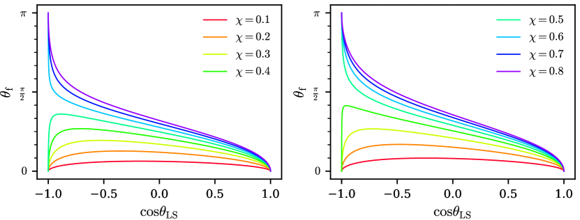
Figure 1: Evolution of the final spin inclination $\theta_{\mathrm{f}}$ with the inclination of the initial spin of the binary $\chi$. The left hand panel shows binaries with a mass ratio $q=6$, while the right hand panel shows those with mass ratio $q=8$. The aligned-spin limit transitions from $\theta_{\mathrm{f}}=0$ to $\theta_{\mathrm{f}}=\pi$ when $\chi\sim 0.55$ for $q=6$ and $0.42$ for $q=8$– when the aligned component of the final spin is zero, as shown in Fig. 2. This transition is now captured in the modeling of the merger-ringdown precession angle $\beta$.

The precession angles that describe the rotation of the dominant multipole from the coprecessing frame into the $\mathbf{J}$-frame take the same form as described in detail in Paper I ​. In brief, during inspiral the precession angles $\alpha$ and $\beta$ are given by the MSA angles outlined in Ref. Chatziioannou et al. (2017). The angle $\beta$ is rescaled using a PN expression so that it describes the precession of the optimal emission direction, rather than the precession of the orbital plane. The rescaling expression is discussed above Eq. (43) in Paper I ​. During merger and ringdown, the angles are given by a phenomenological ansatz fit to data from NR simulations. The two regimes are connected as described in Sec. VIII of Paper I ​. The third precession angle $\gamma$ is then calculated numerically using the minimal rotation condition Boyle et al. (2011).

In this iteration of the model we have recalibrated the merger-ringdown fits against the entirety of the 80 simulations presented in Ref. Hamilton et al. (2023a). These simulations are all single-spin binaries, where the spin is placed on the larger black hole. We therefore use the two-spin mapping outlined in Sec. VII C of Paper I ​ to obtain the form of the merger-ringdown angles for two-spin systems.

We use the same phenomenological form for the merger-ringdown angles as introduced in Paper I ​. These are

$$\alpha\left(f\right)-\langle\alpha\left(f\right)\rangle={} -\left(\frac{A_{1}}{f}+\frac{A_{2}\sqrt{A_{3}}}{A_{3}+\left(f-A_{4}\right)^{2}}\right),$$ (20)

$$\beta\left(f\right)-\langle\beta\left(f\right)\rangle={} \beta\left(f\right)-B_{0}=\frac{B_{1}+B_{2}f+B_{3}f^{2}}{1+B_{4}\left(f+B_{5}\right)^{2}},$$ (21)

where the $A_{i}$ and $B_{i}$ are free coefficients. We now explicitly enforce the non-spinning and (anti-) aligned-spin limits in the expressions of these coefficients. In the case of most of these coefficients, we want the value to tend towards zero as we move into the non-precessing limit. However, $B_{0}$, which represents the overall amplitude of $\beta$ during ringdown, has a more complicated behavior in the non-precessing limit.

Consider an aligned-spin system. In this case, the optimal emission direction and the orbital angular momentum are aligned and both perpendicular to the plane of the binary. $\beta$ therefore measures the angle between the orbital angular momentum $\mathbf{L}$ and the total angular momentum $\mathbf{J}=\mathbf{L}+\mathbf{S}=\left(|\mathbf{L}|+\mathrm{sgn}\left(\mathbf{L}\cdot\mathbf{S}\right)|\mathbf{S}|\right)\mathbf{\hat{L}}$;

$$\cos\beta=\mathbf{\hat{L}}\cdot\mathbf{\hat{J}}={} \mathrm{sgn}\left(|\mathbf{L}|+\mathrm{sgn}\left(\mathbf{L}\cdot\mathbf{S}\right)|\mathbf{S}|\right).$$ (22)

It is therefore obvious that when the spin of the binary is aligned with the orbital angular momentum, we have $\beta=0$. However, in the case that the spin and the orbital angular momentum are anti-aligned, if $|\mathbf{L}|>|\mathbf{S}|$, then $\beta=0$ as before, but if $|\mathbf{L}|<|\mathbf{S}|$ then $\beta=\pi$.

For us to be able to apply this intuition to precessing systems, we would need to know the magnitude of the orbital angular momentum just prior to merger. Since this is a poorly defined quantity in the non-linear regime, it is not possible to directly infer the behavior of $\beta$ as it tends towards the anti-aligned-spin limit. Instead, we use the estimate of the final spin direction, relative to the direction of the orbital angular momentum.

Figure 2: Variation of the value of initial binary spin $\chi$ at which the aligned component of the final spin goes to zero. Shown in dotted black are configurations with $q=8,6,4$, shown from left to right. Capturing the correct limiting behavior of $\beta$ is therefore particularly important to model precessing systems with higher mass ratio.

The final spin for a precessing binary is calculated by combining the aligned component $\chi_{\mathrm{f}}^{\parallel}$ obtained from numerical fits for aligned-spin binaries and the in-plane component $\chi_{\mathrm{f}}^{\perp}$, which is assumed to be conserved throughout the evolution of the binary. We use the aligned-spin fits given in Ref. Jiménez-Forteza et al. (2017) with the aligned-spin component given by our single-spin mapping: $\chi_{1}^{\parallel}=\chi\cos\theta_{\mathrm{LS}}$; $\chi_{2}^{\parallel}=0$. The inclination of the final spin relative to the orbital angular momentum just prior to merger is then given by

$$\cos\theta_{\mathrm{f}}={} \frac{\chi_{\mathrm{f}}^{\parallel}}{\chi_{\mathrm{f}}},$$ (23)

where

$$\chi_{\mathrm{f}}={} \sqrt{\left(\chi_{\mathrm{f}}^{\parallel}\right)^{2}+\left(\left(\frac{q}{1+q}\right)^{2}\chi_{\mathrm{f}}^{\perp}\right)^{2}}.$$ (24)

For an aligned spin binary, we find $\chi_{f}=|\chi_{\mathrm{f}}^{\parallel}|$ so $\cos\theta_{\mathrm{f}}=\pm 1$ and so recover the correct limit. We find the transition in limiting behavior occurs when $\chi_{\mathrm{f}}^{\parallel}=0$. This is demonstrated in Figs. 1 and 2. The mean value of $\beta$ in the merger-ringdown regime, $B_{0}$ is modeled as a perturbation on top of the final spin inclination.

Having now established the correct limiting behavior of the precession angles, the coefficients in Eqs. (20) and (21) are given by

$$A_{1}={} \chi\sin\theta_{\mathrm{LS}}\left(\Lambda^{A}_{1}\right)^{2},$$ (25)

$$A_{2}={} -\chi\sin\theta_{\mathrm{LS}}\left(\Lambda^{A}_{2}\right)^{2},$$ (26)

$$A_{3}={} \left(\Lambda^{A}_{3}\right)^{2},$$ (27)

$$A_{4}={} \left(\Lambda^{A}_{4}\right)^{2},$$ (28)

$$\langle\beta\rangle=B_{0}={} \theta_{f}-\chi\sin\theta_{\mathrm{LS}}\Lambda^{B}_{0},$$ (29)

$$B_{1}={} \chi\sin\theta_{\mathrm{LS}}\exp\left(\Lambda^{B}_{1}\right),$$ (30)

$$B_{2}={} -\chi\sin\theta_{\mathrm{LS}}\exp\left(\Lambda^{B}_{2}\right),$$ (31)

$$B_{3}={} \chi\sin\theta_{\mathrm{LS}}\left(\exp\left(\Lambda^{B}_{3}\right)-200\right),$$ (32)

$$B_{4}={} \left(\Lambda^{B}_{4}\right)^{2},$$ (33)

$$B_{5}={} -\left(\Lambda^{B}_{5}\right)^{2},$$ (34)

where the $\Lambda^{X}_{i}$ are a 3-dimension polynomial expansion of the form given by

$$\Lambda^{X}_{i}={} \sum_{p=0}^{3}\sum_{q=0}^{3}\sum_{r=0}^{4}\lambda^{i}_{pqr}\eta^{p}\chi^{q}\cos^{r}\theta_{\textrm{LS}},$$ (35)

(see Eq. (50) in Paper I for reference). Further information on the values of the coefficients $\lambda^{i}_{pqr}$ can be found in Appendix A.

IV.1.2 Checks and fallback behavior for $\alpha$ and $\beta$

As has been previously noted Pratten et al. (2021), in certain parts of the parameter space, the MSA expressions used for $\alpha$ and $\beta$ during inspiral fail. In the case that these angles fail to generate, we use the next-to-next-to-leading-order (NNLO) angles Bohe et al. (2013) instead (for explicit expressions see e.g. Pratten et al. (2021)), as has been done in previous models which employ the MSA angles Pratten et al. (2021). The NNLO expressions for the inspiral angles are then treated exactly as described in the preceding subsection– i.e. rescaling, two-spin mapping and connecting to the merger-ringdown expressions.

Considering $\alpha$, as shown in e.g. the left-most panel of Fig. 5, we see physically incorrect behavior for $A_{1}<0$ ($\alpha$ would decrease as a function of frequency) or $A_{2}>0$ (the dip in $\alpha$ would have the wrong sign). As it is only a small region of parameter space in which this might happen, we enforce the conditions that $A_{1}>0$ by taking the absolute value of the coefficients with the appropriate sign. For $A_{2}$ we replace any positive values with zero. Pathological behavior occurs for $A_{3}<0$. We limit $A_{3}$ to have a value above $10^{-5}$ in order to prevent the dip from becoming unphysically narrow. Finally, in order to ensure that the dip in $\alpha$ does not become unphysically deep, we enforce the following condition; $A_{2}<-\pi^{2}\sqrt{A_{3}}$.

For $\beta$, we impose the following checks. First, we use an $\arctan$ window around $\beta$ to ensure it is bounded between $0$ and $\pi$ (see Eq. (62) and surrounding discussion in Paper I for further details). This ensures that it maintains a physically meaningful value. To ensure that $\beta$ does not become pathological, if $B_{4}\leq 175$ then we use $B_{4}=175$. We determine the correct root of $\beta$ following the prescription set out in Sec. VI D of Paper I ​. With the refitting of the coefficients, we also give an updated condition for Eq. (69) in Paper I ​. This condition now reads:

$$\frac{b}{3a}>\frac{B_{5}}{2}-\frac{2141}{90988}.$$ (36)

The ansatz for $\beta$ can take 3 possible morphologies demonstrated in Fig. (10) in Paper I ​. In the left-hand and center panels, the inflection point occurs at a higher frequency than the maximum ($f_{\mathrm{inf}}>f_{\mathrm{max}}$). In the center panel, the minimum occurs at a higher frequency than the maximum ($f_{\mathrm{min}}>f_{\mathrm{max}}$). In either case, if the maximum occurs above a cutoff frequency $f_{\mathrm{low}}$, then the connection frequency is given by Eq. (57) in Paper I ​​. Otherwise, the connection frequency is just $f_{\mathrm{low}}$, which is defined by Eq. (58) in Paper I ​. In the third case (the right hand panel) the connection frequency is defined to be

$$f_{\mathrm{c}}=\begin{cases}f_{\mathrm{min}}-0.03&{}f_{\mathrm{min}}\geq 0.06\\ \frac{3}{5}f_{\mathrm{min}}&{}f_{\mathrm{min}}<0.06\end{cases}.$$ (37)

In the cases shown in the center and right-hand panels of Fig. (10) in Paper I ​, we set the ringdown value of $\beta$ to be constant, given by the value of the merger-ringdown ansatz at that point. This occurs when $f_{\mathrm{min}}>f_{\mathrm{inf}}$. For cases like the one on the left-hand panel, we allow $\beta$ to taper to its asymptotic value. To do this we set the connection frequency to $100$.

We only evaluate rescaled inspiral $\beta$ without attaching merger-ringdown contribution in cases where: (i) The lower (inspiral-merger) connection frequency is negative. This is done by setting both connection frequencies to $100$. (ii) The lower connection frequency is less than 0.0009. (iii) The value of the merger-ringdown model of $\beta$ is negative at the lower connection frequency. (iv) We find ourselves choosing the wrong root of the expression for the merger-ringdown value of $\beta$. This is determined by identifying cases where the value of the merger-ringdown model at the lower connection frequency is greater than $5\left(\langle\beta\rangle+0.5\right)$.

IV.1.3 Outside the calibration region

Outside the calibration region, we enforce a smooth turnoff of the precession angles so that the model transitions to the inspiral expression for $\alpha$ and the PN-rescaled expression for $\beta$. This is done using a windowing function of the form of Eq. (5), which was

$$w(x)={} \frac{1}{2}\left[\cos\left(\frac{x-x_{b}}{x_{w}}\right)+1\right],$$ (38)

where $x$ is the variable to which we apply the window, $x_{b}$ is value of the variable at the boundary of the window and $x_{w}$ is the range of the values of the variable over which the window is applied. This is the same functional form as is used to turn off the coprecessing tuning outside the calibration region.

For the angles, we smoothly transition to the PN form of the angles once the mass ratio $q$ and single-spin mapped dimensionless spin magnitude $\chi$ are beyond the calibration region. The final window applied to the model is therefore a product of these two windows (i.e. $w(q)w(\chi)$). The parameters used in the two windowing functions are

$$q_{b}=8.5,{} \qquad q_{w}=3.5,$$ (39)

$$\chi_{b}=0.85,{} \qquad\chi_{w}=0.35.$$ (40)

The final expression for the angles in this transition window are

$$\alpha={} w(q)\,w(\chi)\,\alpha_{\mathrm{MR}}+\left[1-w(q)w(\chi)\right]\alpha_{\mathrm{MSA}},$$ (42)

$$\beta={} w(q)\,w(\chi)\,\beta_{\mathrm{MR}}+\left[1-w(q)w(\chi)\right]\beta_{\mathrm{PN}},$$ (43)

where $\alpha_{\mathrm{MR}}$ and $\beta_{\mathrm{MR}}$ are the phenomenological expressions for the merger-ringdown angles, $\alpha_{\mathrm{MSA}}$ is the inspiral expression for $\alpha$ and $\beta_{\mathrm{PN}}$ is the PN-rescaled expression for $\beta$.

IV.2 Final $\beta$

In addition to the fit of the angle $\beta$ in the merger-ringdown regime, which implicitly gives the value to which $\beta$ drops after merger, we find it useful to produce an independent fit of this ringdown value. The value from this independent fit is used in calculating the effective ringdown frequency via Eq. (9). This value is given by a fit

$$\beta_{\mathrm{f}}={} \theta_{f}-\chi\sin\theta_{\mathrm{LS}}\Lambda^{B}_{\mathrm{f}},$$ (44)

where $\Lambda^{B}_{\mathrm{f}}$ is given by Eq. (35). From this it can be seen that as with $\langle\beta\rangle$, we use $\theta_{\mathrm{f}}$ (shown in Fig. 1) to inform the overall shape of $\beta_{\mathrm{f}}$ and the anti-aligned-spin limit in particular. Details on the fit coefficient values is found in Appendix A.

A comparison of the final value of $\beta$ as given by Eq. (44) and that employed by other models is shown in Fig. 3. We compare here against SEOBv5 Ramos-Buades et al. (2023) (right hand panel) and TPHM Estellés et al. (2022) (middle panel) which both set the ringdown value of $\beta$ to a constant equal to the value of the inspiral angle prescription at a specified attachment time. We do not consider XPHM (MSA), where the inspiral angles are employed through merger and ringdown and do not tend to a constant value or XPHM-ST (Spin Taylor), which tends smoothly to either 0 or $\pi$ as determined by the PN treatment of the inspiral angles.

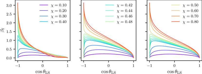
Figure 3: Comparison of $\beta_{\mathrm{f}}$ values between different models. Left: XO4a, center: TPHM, right: SEOBv5. Systems under consideration all have $q=8$.

It can clearly be seen from this figure that both SEOBv5 and TPHM tend to overestimate the ringdown value of $\beta$ since they do not capture the rapid drop in the value at merger. This difference in the values may also be partially accounted for by differences between the time-/frequency-domain values of $\beta$. However, all three models show roughly the same behavior in the antialigned-spin limit in that they tend either to 0 or $\pi$ depending on the binary configuration. The exact point at which this transition occurs differs slightly between the models depending on the approximations employed (XO4a relies on an approximation of the precessing final spin and remnant quantity fits to NR data whereas SEOBv5 and TPHM use PN information from the inspiral). These differences may cause differences when using the various models for data analysis, e.g., parameter estimation for high-mass signals.

IV.3 Additional Changes

IV.3.1 Enforcement of the Kerr limit

The XPHM model includes a check to make sure that the individual spin components do not exceed the physical Kerr limit. In our mapping of generic spins to an equivalent single-spin configuration, there are regions of parameter space where the effective single-spin magnitude exceeds one. This is fine: the parameter no longer represents the physical spin of a single black hole, but an effective spin parameter in the model. As such, the Kerr-limit test in the code to populate the IMRPhenomXPrecessionStruct is bypassed in the special case of producing equivalent single-spin precession angles for these cases.

IV.3.2 Re-mapping of $\theta_{\text{JL}}$

In LAL, the source frame is the frame instantaneously tracking the direction of the orbital angular momentum at the specified reference frequency Schmidt et al. (2017). This frame is related to the $\mathbf{J}$-frame in which the inertial waveform multipole moments are defined by the two angles $(\theta_{\text{JL}},\varphi_{\text{JL}})$, where

$$\theta_{\text{JL}} =\arccos\left(\mathbf{\hat{J}}\cdot\mathbf{\hat{L}}\right),$$ (45)

$$\varphi_{\text{JL}} =\arctan\left(\frac{S_{y}}{S_{x}}\right),$$ (46)

with components defined in the LAL source frame. The expression for $\varphi_{\text{JL}}$ follows from the fact that $\mathbf{\hat{L}}=\mathbf{\hat{z}}$ in the LAL source frame.

When modeling the $\mathbf{J}$-frame signal using our angle model, we are no longer mapping from a source frame determined by the dynamics but rather by the maximal emission direction, $\mathbf{\hat{V}}=\mathbf{\hat{z}}$, in which case the angle $\theta_{\text{JL}}$ as computed in Eq. (45) is not necessarily correct. Instead, the angle $\theta_{\text{JV}}=\beta$ should be used to map from the “maximal emission” source frame in which the spins are defined to the $\mathbf{J}$-frame.

IV.4 Mapping of precession angles to subdominant multipoles

As discussed in Sec. II, complications arise when attempting to extend the same modeling assumptions used to produce the quadrupolar precession angles to higher signal multipoles. The notion that we can simply use the $\ell=2$ Euler angles for the higher multipoles (as one can in the time domain Varma et al. (2019b)) dissolves, and we choose to instead produce a set of angles for each $(\ell,m)$-multipole included in the model.

Furthermore, as seen in Fig. 4, application of the inspiral frequency rescaling is not sufficient to capture the full frequency evolution of the higher multipole precession angles. For this example we compute the FD precession angles $(\alpha_{22},\beta_{22})$ and $(\alpha_{33},\beta_{33})$ from the the FD strain containing only $(\ell,|m|)=(2,2)$ and $(\ell,|m|)=(3,3)$ in the coprecessing frame, respectively. At low frequencies, the simple frequency rescaling with azimuthal index works well, demonstrated by the good agreement of the $\alpha_{22}(2f/3)$ and $\beta_{22}(2f/3)$ curves compared directly to $\alpha_{33}$ and $\beta_{33}$ in Fig. 4. This simple map does not work at high frequencies, where instead the high-frequency behavior of the precession angles appears to be approximately governed by a shift in the input frequency equal to the difference of the $(2,2)$- and $(3,3)$-multipole ringdown frequencies in the coprecessing frame. The transition from depending on $m$ in the inspiral to depending on $\ell$ (through the ringdown frequency scaling) in the merger and ringdown should not come as a surprise, as it follows similarly to the approximate scalings seen in the higher signal multipoles London et al. (2018).

We now discuss the specific details in mapping the tuned precession angles detailed above to the higher multipoles.

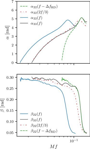
Figure 4: The $\alpha$ and $\beta$ precession angles computed from the $(q,\chi,\theta_{\text{LS}})=(8,0.6,30^{\circ})$ simulation shown in the top and bottom panels, respectively. The angles $\alpha_{\ell\ell}$ and $\beta_{\ell\ell}$ are computed from the FD strain with only $(\ell,\ell)$-multipole moments in the coprecessing frame, for $\ell\in\{2,3\}$. The red dash-dotted curves show the quadrupolar $\ell=2$ precession angles remaped using the approximate inspiral frequency scaling, whereas the green dashed curves show the quadrupolar precession angles shifted in frequency by the difference of the ringdown frequencies $\Delta f_{\text{RD}}=f_{\text{RD},33}-f_{\text{RD},22}$.

IV.4.1 $(\ell,m)$-angle frequency map

To map the tuned, dominant $(2,2)$-multipole precession angles to rotate the higher multipoles, we follow a similar approach as detailed in Ref. London et al. (2018). At low frequencies, the frequency is rescaled with respect to $m$ and the inspiral contributions to the angle functions are evaluated at the velocity

$$v=(2\pi Mf/m)^{1/3},$$ (47)

much as is done in previous precessing higher-multipole Phenom models Khan et al. (2020); Pratten et al. (2021).

At the higher frequencies of the merger and ringdown, the simple inspiral rescaling does not hold and we instead shift the frequency so that each multipole’s ringdown frequency is shifted to the $(2,2)$ ringdown frequency

$$f\rightarrow f-(f_{\text{RD},\ell m}-f_{\text{RD},22}).$$ (48)

The two regions are then connected by a linear mapping between them.

A mapping of the tuned precession angles to rotate the $(\ell,m)$-multipole coprecessing signal is created by evaluating the PNR angles using the frequency map described above, e.g.,

$$\alpha_{\ell m}(f)\equiv\alpha(f_{22}(f)),$$ (49)

with

$$f_{22}(f)=\left\{\begin{array}[]{ll}2f/m&\quad f\leq f_{\text{PN}}\\ \xi_{1}\left(f-f_{\text{PN}}\right)+\xi_{0}&\quad f_{\text{PN}}<f\leq f_{\text{MR}}\\ f-(f_{\text{RD},\ell m}-f_{\text{RD},22})&\quad f>f_{\text{MR}},\end{array}\right.$$ (50)

and linear coefficients,

$$\xi_{1} =\frac{f_{\text{MR}}-(f_{\text{RD},\ell m}-f_{\text{RD,22}})-2f_{\text{PN}}/m}{f_{\text{MR}}-f_{\text{PN}}},$$ (51)

$$\xi_{0} =2f_{\text{PN}}/m.$$ (52)

We specify the lower and upper connection frequencies, $f_{\text{PN}}$ and $f_{\text{MR}}$ respectively, based on connection frequencies defined for both PNR $\alpha$ and $\beta$,

$$f_{\text{PN}} =c_{\text{PN}}\,m\,f_{1}/2,$$ (53)

$$f_{\text{MR}} =c_{\text{MR}}\left(f_{\text{c}}+f_{\text{RD},\ell m}-f_{\text{RD,22}}\right),$$ (54)

where $f_{1}=2A_{4}/7$ and $f_{\text{c}}$ is defined in Eq. (57) of Paper I ​. The coefficients $c_{\text{PN}}$ and $c_{\text{MR}}$ are found by minimizing the joint RMS error between the NR angles and frequency-mapped PNR angles, added in quadrature, for both $\alpha$ and $\beta$ separately. The values of $c_{\text{PN}}=0.65$ and $c_{\text{MR}}=1.1$ were found to be a good initial global fit, and any further tuning with dependence on intrinsic parameters is left for future work. An example comparison of the angles $\alpha_{\ell m}$ and $\beta_{\ell m}$ against NR precession angles is shown in Fig. 5.

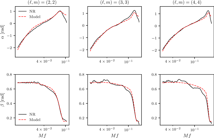
Figure 5: Comparison of the $\alpha_{\ell\ell}$ and $\beta_{\ell\ell}$ precession angles computed from the $(q,\chi,\theta_{\text{LS}})=(4,0.8,90^{\circ})$ simulation for $\ell\in\{2,3,4\}$.

We note one subtle issue with the angle frequency map. If we are to re-map the precession angles by analogy with each multipole’s frequency evolution, as described above, then for consistency the anti-symmetric (2,2) contribution would be rotated with the same angles as the (2,1) multipole, since that most closely mimics the frequency evolution of the antisymmetric (2,2) contribution Ghosh et al. (2023). We experimented with using both the (2,2) and (2,1) angles, and found no appreciable difference in the accuracy with either choice. In this version of the model we have used the (2,2) angles, but this should be reconsidered in future work.

IV.4.2 $(\ell,m)$-angle interpolation

To compute the angles for the higher multipoles as in Eq. (49) we use the cubic spline interpolant provided by the GNU Scientific Library (gsl) Galassi and Gough (2009). This construction requires us to first produce the tuned PNR precession angles $\alpha$, $\beta$, and $\gamma$ over the frequency values used in the frequency map in Eq. (50) and with appropriate frequency spacing.

Given a waveform generated between the frequency values $f_{\text{min}}$ and $f_{\text{max}}$, the frequency map in Eq. (50) potentially requires use of the tuned precession angles outside of the specified frequency range $f\in[f_{\text{min}},f_{\text{max}}]$. To see this one need only look at the mapping for low frequencies $f<f_{\text{PN}}$, where the lowest value is $f_{22}(f_{\text{min}})=f_{\text{min}}/2$ for the $(4,4)$-multipole angles. At high frequencies $f>f_{\text{MR}}$, it is possible for $f_{22}(f_{\text{max}})>f_{\text{max}}$ when mapping to the $(2,1)$-multipole, where generally $f_{\text{RD},21}<f_{\text{RD},22}$. This extension to the frequency range must be accounted for to avoid extrapolation errors in the spline evaluation.

To appropriately generate interpolants that will cover the required frequency range, we specify modified minimum and maximum frequency values, $\breve{f}_{\text{min}}$ and $\breve{f}_{\text{max}}$ respectively, between which we generate the angles. For the minimum frequency, we set $\breve{f}_{\text{min}}=2f_{\text{min}}/m$ for the largest value of $m$ contained in the list of signal multipoles desired in the waveform. To compute the maximum frequency, we specify $\breve{f}_{\text{max}}=f_{\text{max}}-(f_{\text{RD},21}-f_{\text{RD,22}})$ if the $(2,1)$-multipole is desired; otherwise we keep $\breve{f}_{\text{max}}=f_{\text{max}}$.

Finally, once we are equipped with the appropriate frequency spacing $\Delta f$ (see below), we pad the minimum and maximum frequencies by $2\Delta f$ to avoid potential extrapolation due to truncation errors. Should $\breve{f}_{\text{min}}-2\Delta f<0$, then $\breve{f}_{\text{min}}$ is close to zero and we instead take half of the minimum frequency $\breve{f}_{\text{min}}/2$.

Generation of the precession angles used to construct the cubic spline interpolants is done on a uniform frequency grid; we now describe the methods used to estimate an appropriate frequency spacing for that uniform frequency grid, following loosely the work done on frequency multibanding of the gravitational wave phasing and precession angles detailed in Refs. García-Quirós et al. (2021); Pratten et al. (2021).

We initially consider single-spin cases, or cases for which two-spin interactions are negligible, and work in units where the total mass $M=1$. In these cases, as discussed in Sec. VD of Pratten et al. (2021), the most stringent requirement on $\Delta f$ arises from the behavior of $\alpha$ in the inspiral, which at leading PN order scales with frequency as,

$$\alpha\sim\left(-\frac{5\delta}{64m_{1}}-\frac{35}{192}\right)(\pi f)^{-1}.$$ (55)

The work in García-Quirós et al. (2021) considers linear interpolation of the gravitational wave phase and amplitude, and relates in their Eq. (2.5) the frequency spacing $\Delta f$ required to produce an interpolant with a given error $R$ to the second derivative of the function being interpolated. In this work we are using cubic spline interpolants with natural boundary conditions, and we may therefore assume that the error scaling in this interpolation is approximated by Hall and Meyer (1976),

$$R(f_{*})\leq\max_{f_{0}\leq f_{*}\leq f}\frac{5}{384}\alpha^{(4)}(f_{*})\Delta f^{4},$$ (56)

for some $f_{0}<f_{*}<f$.

Solving for $\Delta f$ and using Eq. (55), we find,

$$\Delta f=4\sqrt{\frac{2}{5}}\left(\frac{3\pi R\left[1+\sqrt{1-4\eta}\right]}{7+13\sqrt{1-4\eta}}\right)^{\frac{1}{4}}(\breve{f}_{\text{min}})^{\frac{5}{4}},$$ (57)

where we have used $m_{1}=(1+\delta)/2,$ $\delta=\sqrt{1-4\eta}$, and the fact that the fourth derivative Eq. (55) will be maximized for a given set of parameters at the lowest evaluated frequency $\breve{f}_{\text{min}}$. For the purposes of mapping the higher-multipole angles, we set the default value of $R=0.01$, though this error threshold may be modified using the LALSimulation waveform flag infrastructure (see Appendix A).

While the angle model was tuned to single-spin configurations, the MSA precession angles used for frequencies covering the inspiral regime describe generic two-spin configurations and may contain oscillations induced by changes in the magintude of the total spin vector. In these cases the above frequency spacing specified by Eq. (55) may not suffice and we turn to a different method to predict the required spacing. The oscillations in the total spin magnitude are given by Chatziioannou et al. (2017),

$$S_{0}^{2}=S_{+}^{2}(t_{\text{rr}})+\left[S_{-}^{2}(t_{\text{rr}})-S_{+}^{2}(t_{\text{rr}})\right]\text{sn}[\psi(t_{\text{pr}},t_{\text{rr}}),m(t_{\text{rr}})],$$ (58)

where $S_{-}^{2}$ and $S_{+}^{2}$ are the squared magnitudes of the minimum and maximum total spin vector configurations, respectively, $t_{\text{rr}}$ is the radiation-reaction timescale, $t_{\text{pr}}\ll t_{\text{rr}}$ is the precession timescale, $\psi$ is the phase angle tracking the oscillation between $S_{-}$ and $S_{+}$, and $m=(S_{+}^{2}-S_{-}^{2})/(S_{+}^{2}-S_{3}^{2})$.

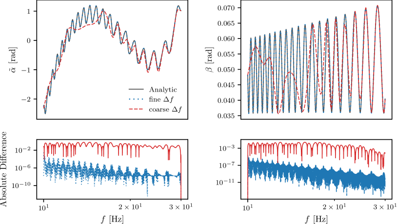
Figure 6: Comparison between the analytic evaluation of $\alpha$ and $\beta$ and two interpolants generated with different frequency resolutions, “fine $\Delta f$” from Eq. (62) and “coarse $\Delta f$” from Eq. (57), for the case detailed in Table 1. The top panels show plots of the precession angles, where we have defined $\tilde{\alpha}$ to be the difference between $\alpha$ and a quadratic polynomial fit to the analytic $\alpha$ to better facilitate visualiztion of the two-spin oscillations. The bottom panels show the absolute difference between the analytic angles and the interpolants when evaluated on the same frequency grid as the analytic angles. Here the red solid curves correspond to the difference between the analytic angles and coarsely-sampled interpolants, and the blue dashed curves show the difference between the analytic angles and finely-sampled interpolants.

The solution for $\psi$ is given by Eq. (51) of Chatziioannou et al. (2017),

$$\psi=\psi_{0}-\frac{3g_{0}\delta m}{4}v^{-3}\left(1+\psi_{1}v+\psi_{2}v^{2}\right),$$ (59)

where $\psi_{0}$ is a constant of integration, $v$ is the velocity defined in Eq. (47), and the remaining terms are defined in Chatziioannou et al. (2017). We will assume that over a small range of frequency values close to $\breve{f}_{\text{min}}$, we can approximate

$$\text{sn}[\psi(\breve{f}_{\text{min}}),m]\approx\sin(\psi^{\prime}\breve{f}_{\text{min}}),$$ (60)

where $\psi^{\prime}$ is the first derivative of Eq. (59) with respect to $f$,

$$|\psi^{\prime}|=\frac{\pi g_{0}\delta m}{4v^{6}}\left(3+2\psi_{1}v+\psi_{2}v^{2}\right).$$ (61)

Then to adequately resolve the oscillations in Eq. (60) we choose to specify a sampling rate that places four frequency points within one period of oscillation, i.e.,

$$\Delta f=\frac{1}{4|\psi^{\prime}|}.$$ (62)

This approximation handles almost all cases of two-spin oscillations. For some configurations where the minimum and maximum values of $\beta$ satisfy $0\approx\beta_{\text{min}}<\beta_{\text{max}}$ we see sweeping oscillations in $\beta$ that drop close to zero, at which point the coordinates of the rotation approach a singular point and $\alpha$ sees sharp jumps of $\pi$. To predict these cases we compute the minimum and maximum values that $\beta$ can take following Pratten et al. (2021),

$$\beta_{\text{min}} =\arctan\left(\frac{|S_{1\perp}-S_{2\perp}|}{L+S_{\parallel}}\right),$$ (63)

$$\beta_{\text{max}} =\arctan\left(\frac{S_{1\perp}+S_{2\perp}}{L+S_{\parallel}}\right),$$ (64)

where $L$ is the magnitude of the post-Newtonian orbital angular momentum used by XPHM evaluated at $\breve{f}_{\text{min}}$, $S_{\parallel}$ is the component of the total spin parallel to $\mathbf{L}$, and $S_{1,2\perp}$ are the components of $\mathbf{S}_{1}$ and $\mathbf{S}_{2}$ perpendicular to $\mathbf{L}$, respectively.

When the conditions $\beta_{\text{min}}<0.01$ and $\beta_{\text{min}}/\beta_{\text{max}}<0.55$ are both met, then we can assume that $\beta$ is oscillating sufficiently close to zero for jumps in $\alpha$ to be a potential concern. In this case, we increase the resolution by dividing $\Delta f$ in Eq. (62) by a factor of 4,

$$\Delta f=\frac{1}{16|\psi^{\prime}|}.$$ (65)

Finally, we use the minimum $\Delta f$ computed from either Eqs. (57),  (62), or (65), and require that the final choice of $\Delta f\geq 10^{-2}$ so as not to saturate available memory when generating the waveform.

Parameter	Value
$M$ [$M_{\odot}$]	34.7488472
$q$	15.1486886
$\chi_{1}$	$(-0.04585042,-0.03174999,0.65327636)$
$\chi_{2}$	$(-0.90498966,0.31916086,-0.06208559)$

Table 1: Configuration used to generate Fig. 6. The angles were produced with starting and reference frequencies of 10 Hz.

In Fig. 6 we show the impact of inadequate frequency spacing on the interpolation of the oscillating precession angles. The precession angles $\alpha$ and $\beta$ are presented in the top two panels of the figure for the configuration listed in Table 1, where the analytic evaluation of the angles with $\Delta f=1\times 10^{-3}$ Hz is shown in black solid curves. The blue dotted and red dashed lines show the results of inerpolating the analytic $\alpha$ and $\beta$ using the frequency step sizes given in Eqs. (62) ($\Delta f=0.027$ Hz) and (57) ($\Delta f=0.843$ Hz), respectively. To more clearly show the oscillatory behavior of $\alpha$, we define $\tilde{\alpha}$ to be $\alpha$ minus a quadratic polynomial fit to the analytic evaluation of $\alpha$, thereby removing the dominant $f^{2}$ growth of the angle with frequency.

Unsurprisingly, the oscillations in $\alpha$ and $\beta$ require finer frequency spacing to be accurately resolved compared to the simple leading-order-in-frequency estimate provided from Eq. (57). This can be seen quite clearly from the absolute differences between the interpolants and the analytic angles displayed in the lower panels of Fig. 6. As the period of the two-spin oscillations eventually increases enough for the coarse frequency resolution to resolve the oscillations (at roughly the highest frequencies plotted in Fig. 6), the error from the coarsely-sampled interpolation begins to drop.

V Model Performance and PE Results

We now look to assess the performance of XO4a by means of both mismatches and parameter estimation (PE). We adopt the definitions of the mismatch $\mathfrak{M}$ and precessing mismatch $\mathfrak{M}_{\text{w}}$ discussed in Sec. XI A of Paper I ​​. In computing mismatches we utilize the advanced LIGO power spectral density at design sensitivity LSC .

In Sec. V.1 we first analyze the perfomance of the underlying coprecessing XHM-CP model and also assess the impact of adding the antisymmetric contribution. We then extend our analysis to look at precessing mismatches with symmetrized $(\ell,|m|)=(2,2)$ coprecessing data in Sec. V.2 and full $\ell=2$ coprecessing data in Sec. V.3. Precessing mismatches using all available coprecessing frame multipoles and the mapped HM-angles are presented in Sec. V.4. Finally we give results from PE recoveries performed with XO4a alongside other contemporary models in Sec. V.5.

V.1 Coprecessing frame mismatches

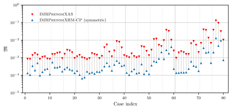
Figure 7: Mismatches $\mathfrak{M}$ computed between the symmetrized $(\ell,m)=(2,2)$ coprecessing NR data tabulated in Table I of Ref. Hamilton et al. (2021) and the symmetric $(\ell,m)=(2,2)$ coprecessing strain generated with the models XHM-CP, shown with upward pointing arrows, and XAS shown with downward pointing arrows.

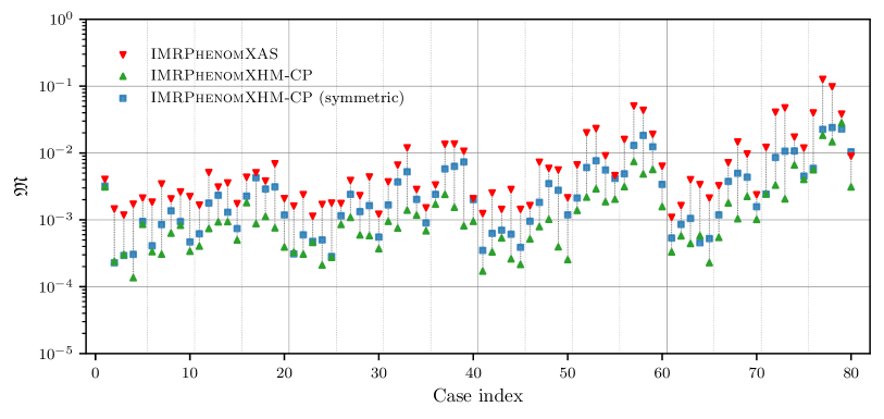
Figure 8: Mismatches $\mathfrak{M}$ computed between the full $(\ell,m)=(2,2)$ coprecessing NR data with antisymmetric contributions tabulated in Table I of Ref. Hamilton et al. (2021) and the $(\ell,m)=(2,2)$ coprecessing strain generated with the models XHM-CP, shown with upward pointing arrows, and XAS shown with downward pointing arrows. Here the NR data is not symmetrized and the antisymmetric contribution to XHM-CP is enabled. We also include the match between the full coprecessing NR and XHM-CP with the antisymmetric contributions to the model disabled, shown as blue squares. The improvement in performance achieved by the addition of the antisymmetric part to the co-precessing waveform is evident.

We start by computing mismatches between the tuned $(\ell,|m|)=(2,2)$ symmetric coprecessing model contribution to XHM-CP and the 80 NR waveforms detailed in Ref. Hamilton et al. (2023a) and compare the results to the modified aligned-spin verson of XAS used in XPHM. All mismatches in this subsection use a total mass of $100\,M_{\odot}$, starting frequency $f_{\text{min}}=\text{min}\,\left\{20\,\text{Hz},f_{\text{ref}}+5\,\text{Hz}\right\}$ and $f_{\text{max}}=1024\,\text{Hz}$.

As an initial result shown in Fig. 7, we verify that the performance improvement seen in Paper I by tuning the dominant quadrupolar contribution to the underlying coprecessing model in DCP is retained in XHM-CP. Across the calibration waveforms we see improvement in the mismatch performance over the coprecessing model used in XPHM for the dominant $(\ell,|m|)=(2,2)$ contribution. This relative improvement is maintained when comparing to the full $(\ell,m)=(2,2)$ NR coprecessing data without symmetrization, shown in Fig. 8. While the mismatches for both XHM-CP and XPHM degrade slightly in overall performance, a majority of the XHM-CP mismatches remain below $10^{-3}$. For this set of matches, the antisymmetric contributions to XHM-CP are enabled, and we optimize the matches over rotations of the in-plane spin direction, thereby optimizing over the antisymmetric phase. Figure 8 nicely demonstrates the improvement in the coprecessing model due to modeling the dominant multipole asymmetry. Notably, for about a third of the cases, mismatches $\sim$$10^{-3}$ were only attainable after adding the model of the antisymmetric waveform to the coprecessing model.

Finally in this section we remark on the performance of the higher multipole contributions to XHM-CP described in Sec. III.1.2, where no tuning has been done but the ringdown frequencies used in each multipole are modified by Eq. (9). Mismatches between individual coprecessing higher multipoles were computed for all 80 NR waveforms (except the $q=1$ configurations for the odd-$m$ multipoles, where the coprecessing contributions approximately vanish). In general the performance improvement is lower compared to the results shown in Fig. 7, which is to be expected as the full tuning to NR has not been done. On average the mismatches improve across the parameter space when using the effective ringdown frequency for each multipole, with larger improvements seen at higher mass-ratios and spin magnitudes, and we report the mean percentage improvement in the mismatches for each $(\ell,|m|)$-multipole: $(2,1)$: $0.09\%$, $(3,3)$: $0.17\%$, $(3,2)$: $0.05\%$, $(4,4)$: $0.14\%$.

We expect that explicit tuning of the higher multipoles could achieve similar levels of accuracy to that achieved for the co-precessing-frame (2,2) multipoles. However, this also requires that the model accurately capture the relative phasing between the multipoles. We will return to this point when we consider full precessing matches in Sec. V.4.

V.2 Symmetrized $h^{\mathrm{CP}}_{22}$ mismatches

We next consider the accuracy of both our underlying symmetric dominant-coprecessing-multipole and of the dominant multipole precession angles to the waveform. As described above, we have calibrated both the symmetric coprecessing (2,2) multipole and the merger-ringdown part of the precession angles $\alpha$ and $\beta$ to a set of 80 NR waveforms Hamilton et al. (2023a). In order to test the performance of this model and the validity of the approximations made, we calculate the full SNR-weighted precessing match between the $\ell=2$ multipoles of the model in the inertial frame and the 80 calibration waveforms.

To do this, we use the cleaned and symmetrized NR waveforms used in the calibration process, more details of which can be found in Paper I ​. The model data are produced by calling XO4a with only the $(2,2)$ multipole activated in the coprecessing frame and the multipole asymmetries turned off. For comparison, we also consider SEOBv5, which is also called with only the $(2,2)$ multipole activated (and natively does not include multipole asymmetries).

When calculating the match, we consider masses in the range between $100\mathrm{M}_{\odot}$ and $240\mathrm{M}_{\odot}$ at intervals of $20\mathrm{M}_{\odot}$. We calculate the match at each of the inclination values in the set $\left\{0,\pi/6,\pi/3,\pi/2\right\}$. The match is performed over the frequency range $f_{\textrm{min}}=\mathrm{max}\{20\,\mathrm{Hz},f^{\mathrm{NR}}_{\textrm{min}}+5\mathrm{Hz}\}$ to $f_{\mathrm{max}}=512$ Hz. This set up is chosen to allow for direct comparison with results in Sec. XI E in Paper I utilizing PNR.

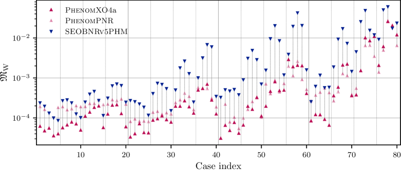
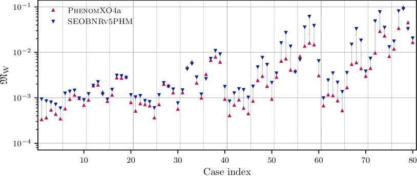
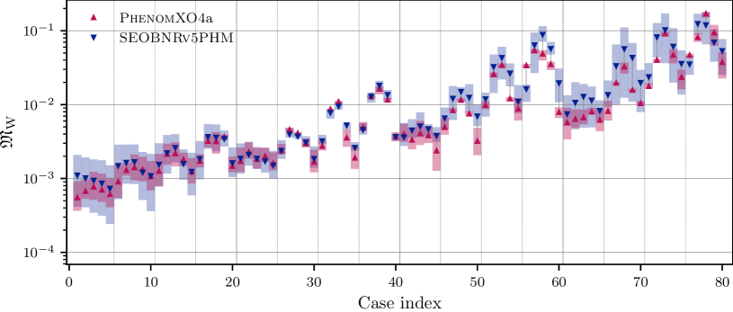
Figure 9: SNR-weighted mismatches in the $\mathbf{J}$-frame between the NR BAM waveforms and the XO4a and SEOBv5 models containing (a) only the $(2,2)$ multipole in the coprecessing frame – against symmetrized NR data (top panel) (b) all available coprecessing frame $\ell=2$ multipoles (middle panel) and (c) all available coprecessing frame multipoles up to $\ell=4$. In the top panel, a comparison with PNR is included for reference. The points are averaged over total mass and inclination; the bars show the spread with total mass.

The results of this comparison can be seen in the top panel of Fig. 9. First, we can see that the improvements to the calibration presented in this paper show an improvement of XO4a over PNR on average across the parameter space. In particular, we see an improvement in the low-spin regime due to the improved treatment of the zero-spin limit in the modeling of the precession angles. It is important to note that PNR was originally calibrated to a subset of just 40 of the numerical waveforms, whereas XO4a has been calibrated to the entire set. Fitting to just a subset of the waveforms with PNR enabled us to check that there was no overfitting or other issues. We then calibrated XO4a against the additional 40 waveforms to further improve accuracy. We note that the performance of PNR for the additional spin magnitudes of $\{0.2,0.6\}$ is consistent with the accuracy achieved for the calibration set (i.e. $\chi=[0.4,0.8]$). This indicates that the good matches seen here are not purely a consequence of comparing to the calibration set of waveforms.

We can also see the effect of the calibration on these matches when compared to SEOBv5, a recent state-of-the-art precessing model which does not calibrate precession effects to NR. XO4a performs better than SEOBv5 across the parameter space, often by an order of magnitude. A comparison for these cases with the older models XPHM and SEOBNRv4PHM can be seen in Paper I ​. We see the same improvement there when comparing a model with calibrated precession effects against those without.

V.3 $\ell=2$ mismatches

We now consider the impact of the inclusion of higher order multipoles and asymmetry on the model accuracy. We first include all $\ell=2$ coprecessing multipoles used in each model. XO4a and SEOBv5 contain the symmetric $(2,\pm 2)$ and $(2,\pm 1)$ multipoles in the coprecessing frame, and XO4a also includes the antisymmetric $(2,\pm 2)$ multipoles. The NR waveforms contain all $\ell=2$ multipoles in the inertial frame without further processing (i.e. no symmetrization). Once again we calculate the full SNR-weighted precessing match in the inertial frame. We consider systems with total mass $\{60,90,120,150\}M_{\odot}$ and inclinations $\{0,\pi/3,\pi/2,2\pi/3,\pi\}$. The match is performed over the frequency range $f_{\textrm{min}}=\mathrm{max}\{20\,\mathrm{Hz},1.35f^{\mathrm{NR}}_{\textrm{min}}\}$ to $f_{\mathrm{max}}=512$ Hz. This is a slightly different set up to that considered in the previous subsection. Since we are now considering the effect of asymmetry on the waveform, we now include inclinations greater than $\pi/2$. As we are examining a greater number of systems than in Paper I we sample the total mass parameter space less densely in order to ensure that the analysis is computationally feasible.

First we consider the performance of XO4a against the set of 80 calibration BAM waveforms, shown in the middle panel of Fig. 9. Here we show the mismatch value averaged over all masses and inclinations. Since these results have been produced using a slightly different set of choices for the total masses and inclinations, they cannot be compared directly with the results for the symmetrized $(2,2)$-only matches shown in the top panel. However, we can see that the mismatch degrades by up to an order of magnitude with the addition of the untuned $(2,1)$ multipoles in the coprecessing frame and when considering the multipole asymmetries. It is unclear which of these additions has the dominant impact on the mismatches. For systems with spin magnitude below 0.4, we see that the mismatches lie below $10^{-2}$ for all cases up to $q=8$. For systems with $q\geq 4$ and spin magnitudes above 0.4, the mismatch value starts to become notable. It is therefore important to improve the calibration of the model in this part of the parameter space. We also consider the performance of SEOBv5 against the same set of waveforms. When considering just the $\ell=2$ multipoles, XO4a still outperforms SEOBv5 in almost all cases. This improved performance is particularly significant for the higher mass ratio cases included in the dataset.

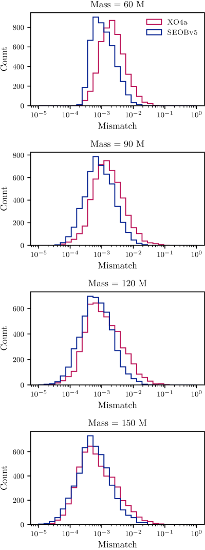
Figure 10: Mismatches between the $\ell=2$ multipoles in the $\mathbf{J}$ frame of NRSur, XO4a and SEOBv5. Considered 1024 two-spin configurations at four different total masses $\{60,90,120,150\}M_{\odot}$ and five different inclinations $\{0,\pi/3,\pi/2,2\pi/3,\pi\}$ rad.

It is worth noting here the uncertainty in the NR waveforms. The mismatch uncertainty in the BAM waveforms is estimated to be $\sim$$10^{-3}$ Hamilton et al. (2023a). We have also calculated mismatches between BAM waveforms and SXS waveforms where equivalent configurations exist, and those results are consistent with the same level of disagreement. We therefore caution against interpreting any significance to mismatch differences that are smaller than this threshold, which is in general the level of improvement between XO4a and SEOBv5 $\ell=2$ mismatch results in the middle panel of Fig. 9 until we reach the cases where $q=4$ and $\chi=0.6$ (above case 50). For example, in mismatch calculations where we replace the BAM waveforms by equivalent NRSur waveforms, we find that the relative performance of XO4a and SEOBv5 often swaps, but changes are not more than roughly $10^{-3}$.

We also consider single-spin NRSur configurations that differ from those in our calibration set, i.e., with spin magnitudes and misalignment angles in between those used for the BAM simulations. We find similar levels of mismatch to neighbouring configurations, again demonstrating that over-fitting is not a significant source of error.

We also consider the performance of these two models against a set of 1024 two-spin configurations generated using NRSur. Due to the region of validity of the surrogate model, these configurations only extend up to mass ratio $q=4$. These results are shown in Fig. 10. From this comparison we can see that in general SEOBv5 slightly outperforms XO4a. A closer inspection of the results shown in Fig. 10 reveals that the performance is roughly comparable between the two models, with a tail extending towards higher mismatches present for XO4a accounting for most of the difference. This effect is less prevalent at higher total mass, where the signal consists of mainly merger and ringdown. From this we can infer that it is likely the inspiral part of XO4a which requires the greatest improvement while the merger-ringdown part has already been accurately tuned.

There are a number of possible reasons for the different pictures of the model accuracy shown in Figs. 9 and 10. First and foremost is the presentation of the data — in Fig. 9 we average over inclination and total mass, while in Fig. 10 we do not, so extremely good/bad cases are more prominent. Secondly, the mismatch uncertainty between BAM and NRSur of $\mathcal{O}(10^{-3})$ is reflected in the performance of the models against three different “datasets.” Finally, the random sampling of the two-spin parameter space in Fig. 10 very rarely samples the large-mass-ratio large-primary-spin cases for which SEOBv5 shows poor matches in Fig. 9. The picture is however consistent when examining calibration and non-calibration cases, so we do not attribute the apparent change in performance to any overtuning of the model. From this we conclude that SEOBv5 slightly outperforms XO4a in the bulk of the parameter space, but is less accurate for more extreme configurations.

V.4 HM Mismatches

Finally, we consider the overall performance of the final model. We use the same match set up as described in the preceding section. We consider a data set consisting of the 80 calibration BAM waveforms and 1024 two-spin configurations generated using NRSur. We compare XO4a with the other contemporary time- and frequency-domain waveform models.

The results of the comparison against the 80 calibration BAM waveforms are shown in the bottom panel of Fig. 9. We can see from a direct comparison with the middle panel (which shows the mismatch results for just the $\ell=2$ multipoles) that the inclusion of the higher order multipoles further degrades the performance of both XO4a and SEOBv5, and we now see that the performance of the two models is roughly comparable.

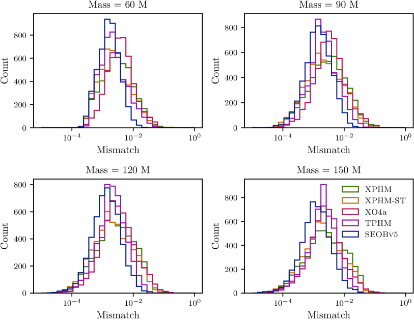
Figure 11: Mismatches between all multipoles up to $\ell=4$ in the $\mathbf{J}$ frame of NRSur and XO4a and SEOBv5. Considered 1024 two-spin configurations at four different total masses $\{60,90,120,150\}M_{\odot}$ and five different inclinations $\{0,\pi/3,\pi/2,2\pi/3,\pi\}$ rad.

To explore the $q\leq 4$ parameter space more thoroughly, we also consider the 1024 configurations generated using NRSur. The results of this study is shown in Fig. 11, from which we can see that for the systems considered in this study, SEOBv5 performs best, followed by TPHM. The frequency-domain models XPHM, with both the MSA and SpinTaylor angles, and XO4a have a tail to larger mismatches which degrade the overall performance of the model. It is our understanding, informed by comparison with Fig. 10 and of the middle and bottom panels in Fig 9, that this arises from the non-trivial nature of the relative phasing of the higher multipoles in the frequency domain, which has not yet been completely understood. Once this issue has been resolved, further tuning to the higher-order multipoles and extending the calibration to two-spin systems is expected to reproduce the improvement seen in the $(2,2)$-only and $\ell=2$ multipoles. (We note that the symmetric $\ell=2$ mismatches shown in Paper I illustrate that tuning each ingredient in a Phenom model can lead in principle to competitive accuracy to NRSurrogate models, but with far fewer input waveforms.) From Fig. 11 we can also see that the broadening of the histograms toward lower mismatches with increased total mass seen for the $\ell=2$ results is not as strong when we consider systems which include higher order multipoles.

We also consider an additional 216 single-spin cases with the spin placed on the large black hole, thus mimicking the data set against which the model was calibrated. A comparison of the performance of the model against the single-spin and two-spin cases shows that the tuning to single-spin systems is not currently the dominant source of error in XO4a, given the comparable performance presented.

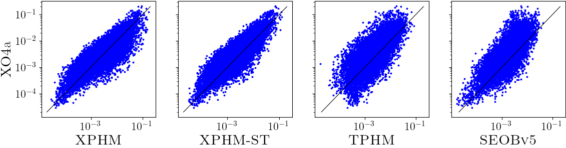
Figure 12: Mismatches between all multipoles up to $\ell=4$ in the $\mathbf{J}$ frame of NRSur7dq4 and selected models. Considered 1024 two-spin configurations at four different total masses $\{60,90,120,150\}M_{\odot}$ and five different inclinations $\{0,\pi/3,\pi/2,2\pi/3,\pi\}$ rad.

An alternative comparison of the performance of XO4a against the other models considered in this study can be seen in Fig. 12. This shows that the time domain models TPHM and SEOBv5 generally perform better than the frequency domain models, which have a roughly comparable performance. However, the improvement does not exceed a factor of $\sim$2 at best. This is consistent with our expectation of the importance of correctly modelling relative phase offsets between multipoles, which is likely incorporated more naturally in time-domain models, where the relative phases are inherited from the PN/EOB approximants.

We also considered the dependence of the mismatch on the inclination of the system. The inclination here is measured with respect to the orbital plane of the binary at the reference frequency. Since these are precessing systems, this will change throughout the evolution of the binary. However, since these systems are uniformly distributed with $q\leq 4$ $|\chi_{1,2}|<0.8$ we do not expect the precession effects to be particularly strong for the majority of these systems — for example, we do not expect to see transitional precession which would cause a strong change in the orientation of the binary during its evolution.

We observe that the spread of mismatch values is greatest for systems that are face-on and face-off at the reference frequency, i.e., both the best and the worst mismatches are seen here. This is true for all models. It is for binaries which are originally edge-on where we see the greatest difference in model performance, with SEOBv5 showing a clear shift towards lower mismatch values compared to the other models, while for originally face-on/off systems the performance of all models is much more comparable for the bulk of systems, though the Phenom models have a noticeable tail to higher mismatches.

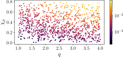
Figure 13: Dependence of the mismatches between all multipoles up to $\ell=4$ in the $\mathbf{J}$ frame of NRSur and XO4a on $q$ and $\chi_{\mathrm{p}}$. Total mass $90M_{\odot}$, averaged over inclination.

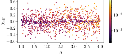
Figure 14: Dependence of the mismatches between all multipoles up to $\ell=4$ in the $\mathbf{J}$ frame of NRSur and XO4a on $q$ and $\chi_{\mathrm{eff}}$. Total mass $90M_{\odot}$, averaged over inclination.

Finally, we consider how the performance of XO4a varies across the parameter space. The dependence on the mass ratio and dominant spin effects is demonstrated in Figs. 13 and 14. From this we can clearly see that XO4a performs best at low mass ratios and low in-plane spin values, as would be expected. The worst mismatches occur for systems with in-plane spin magnitudes above $\sim$0.6, with the very worst of these seen for systems with $q>3$. The dependence on $\chi_{\mathrm{eff}}$ is much less strong, with poorer mismatches seen at all values of $\chi_{\mathrm{eff}}$. The best mismatches predominantly occur for systems with $|\chi_{\mathrm{eff}}|<0.1$.

V.5 Parameter Estimation Results

The mismatch study presented in Sec. V.4 describes the accuracy of XO4a for single points in the parameter space. Although it was found that XO4a performs best at low mass ratios and low in-plane spin values, it only gives limited insight into how XO4a performs for realistic GW applications – for example inferring the properties of the binary through Bayesian inference, e.g. Veitch et al. (2015), and identifying GWs in noise, e.g. Allen et al. (2012); Babak et al. (2013). Previous attempts to correlate the mismatch with the model’s performance for GW applications led to the indistinguishability criterion Baird et al. (2013). Here, the mismatch was shown to relate to an indistiguishability SNR, where biases in parameter estimates may be observed for GWs with SNRs larger than the indistinguishability SNR. We therefore assess the accuracy of XO4a for realistic GW applications by performing Bayesian inference on both synthetic and real GW signals, with our choice of synthetic signal informed by identifying configurations where the SNR is above the indistinguishability SNR for all models. To quantify possible systematic biases, we compare the posterior distribution obtained with XO4a with a) the distributions obtained with XPHM, XPHM-ST, TPHM and SEOBv5, and b) the true source parameters when they are known. We note that although a typical Bayesian analysis compares $\sim 10^{7}$ waveforms over a wide parameter space, we still only consider isolated GW signals. This means that we still only gain limited insight into the overall performance of XO4a over the full 15-dimensional parameter space.

The first two synthetic injections considered are generated with NRSur as it most accurately resembles numerical relativity across its calibrated parameter space Varma et al. (2019b). We injected these signals into zero noise, which reflects the expected distribution when averaged over many different noise realizations. We use the expected detector sensitivities for the advanced LIGO and advanced Virgo GW detectors Aasi et al. (2015); Acernese et al. (2014). For all cases, we perform Bayesian inference with the dynesty nested sampler Speagle (2020), employed via the Bilby parameter estimation software Ashton et al. (2019); Romero-Shaw et al. (2020). All analyses used 1000 live points along with the bilby-implemented rwalk sampling algorithm with an average of 60 accepted steps per MCMC. We consistently used uninformative and wide priors, as defined in Appendix B.1 of Ref. Abbott et al. (2019).

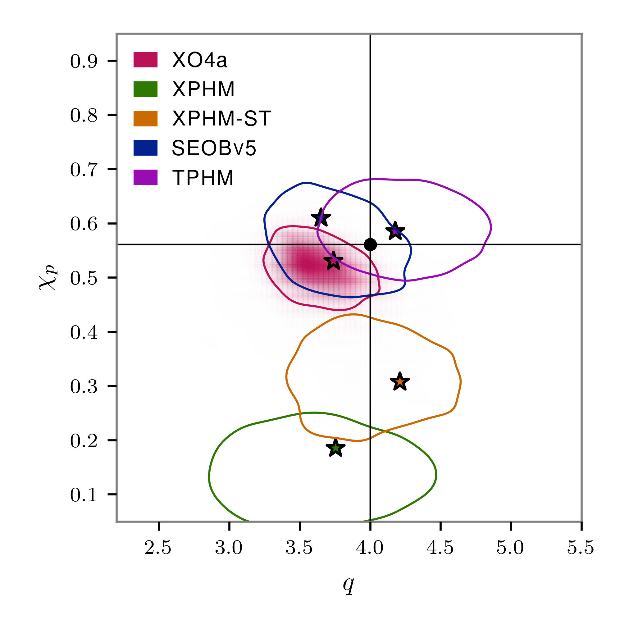
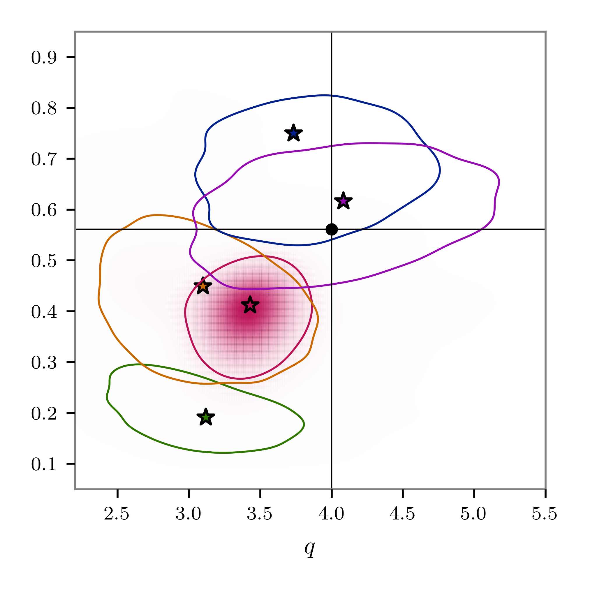
Figure 15: The two-dimensional marginalized posterior distributions for the mass ratio $q$ and effective precessing spin $\chi_{\mathrm{p}}$ when analyzing two gravitational wave signals simulated with NRSur: Left: low mass and Right: high mass. The indicated two-dimensional area shows the inferred 90% credible region, the horizontal and vertical black lines show the injected mass ratio and effective precessing spin, and the markers show the maximum likelihood position. The shaded region indicates the posterior probability density per pixel obtained with XO4a. The low and high mass simulated signals were produced for a binary black system with mass ratios $q=4$, effective spins $\chi_{\mathrm{eff}}=-0.45$, effective precessing spins $\chi_{\mathrm{p}}=0.53$, and total masses $M=60\,M_{\odot}$ and $M=120\,M_{\odot}$ respectively. The distance to the source was chosen so that the simulated signals had signal-to-noise ratio $\mathrm{SNR}=20$.

First, we analyze a synthetic GW signal for a fiducial binary black hole system with total mass $M=60\,M_{\odot}$, mass ratio $q=4$ and dimensionless spin vectors $\chi_{1}=[0.31,0.47,-0.57]$ and $\chi_{2}=[0.37,0.71,0.01]$. The effective spin parameters are $\chi_{\rm eff}=-0.45$ and $\chi_{\rm p}=0.53$. The inclination angle of the binary is set to $\iota=0.98\,\mathrm{rad}$, to emphasize the effect of higher-order multipoles and precession in the signal, and the luminosity distance is chosen to ensure a network SNR of $20$. All other extrinsic parameters are randomly chosen. We perform Bayesian inference on this specific binary configuration as we found a large variance in the match between NRSur and each of the models used in this study at the true source parameters. This is therefore a suitable case to investigate how the matches presented in Sec V.4 translate to performance with Bayesian inference. The mismatches at the true source parameters between NRSur and XPHM, XPHM-ST, XO4a, TPHM and SEOBv5 are 0.040, 0.036, 0.032, 0.018, 0.009 respectively. Based on these mismatch results we would expect only SEOBv5 to be indistinguishable from the injection with 90% confidence; SEOBv5 is the only model with an indistinguishable SNR greater than the injected value. This means that we would expect SEOBv5 to recover the injected values most accurately, with possible biases in the other models.

In Fig 15 we show the inferred two-dimensional marginalized posterior distribution for the mass ratio $q$ and effective precessing spin $\chi_{\mathrm{p}}$ with contours showing the inferred two-dimensional 90% confidence interval (hereafter simply referred to as the 90% confidence interval unless otherwise stated) and maximum likelihood samples. Although we see the general trend that a model with a larger match more accurately recovers the injected value, the trend is not trivial. For instance, although the mismatches for XO4a and both variants of XPHM are comparable and much lower than SEOBv5, the inferred 90% confidence intervals are distinctly different. We see that the inferred distribution obtained with XO4a is comparable to SEOBv5 despite the mismatch being $\sim 3.5\times$ larger. Although all models prefer $q\sim 4$, only XO4a, SEOBv5 and TPHM prefer large in-plane spins; both variants of XPHM show significant biases in the inferred $\chi_{\mathrm{p}}$ with the injected value lying significantly outside of the 90% confidence interval. Although the injected value is outside the 90% confidence region of XO4a, we see that the maximum likelihood samples for XO4a, SEOBv5 and TPHM are similarly spaced around the injected value.

Next, we investigate XO4a’s performance when the total mass of the fiducial binary black hole is increased from $M=60\,M_{\odot}$ to $M=120\,M_{\odot}$. In Fig 15 we see that TPHM recovers the injected values most accurately, with the injected parameters lying within the $50\%$ confidence interval. Judging solely on the inferred 90% confidence interval, we see that SEOBv5 is the next best performing model, with the injected values lying within the 90% confidence interval. All other models show more significant biases, with the injected values lying outside of the inferred posterior distribution. When inspecting the maximum likelihood positions, we see that TPHM recovers a value close to the injected system, while SEOBv5 and XO4a are similarly distributed. We note that the posterior obtained with XO4a is significantly tighter than the other models, which is why it lies outside the 90% confidence region. Assuming that the 90% c onfidence interval scales linearly with SNR Cutler and Flanagan (1994); Poisson and Will (1995) (this approximation is valid in the strong-signal limit), we would expect SEOBv5 to no longer recover the injected value within 90% confidence for a signal with SNR $\sim 22$. When comparing the posterior distributions for the low and high mass cases, we see that for all models the inferred posterior distributions widen. This is expected as more massive binaries merge at lower frequencies, meaning that they have significantly fewer cycles within sensitive region of the detectors and consequently less information to break well known degeneracies. We also see that only XO4a prefers lower in-plane spins, with all other models preferring larger spins than their lower mass counterparts.

In general, we have shown that we cannot rely solely on the point-by-point match results to conclude whether a given model is accurate enough to recover the source properties with Bayesian inference. This is particularly highlighted by the fact that although XO4a’s mismatch for the low mass synthetic injection is $\sim 3.5\times$ larger than SEOBv5, the inferred posterior distribution is comparable. We stress that the matches presented in Sec V.4 are essentially draws from the likelihood surface, and therefore a single point estimate of the true values is not sufficient to understand the full likelihood, and consequently the model’s performance across the full parameter space. This issue may be solved in the future by identifying a more informative mapping between the mismatch and potential biases in parameter estimates, or by sampling over the waveform model and using a parameter space dependent prior that describes the match manifold Hoy (2022). While waveform systematics will likely be an issue for loud GW signals with large mass ratios and in-plane spins, where all models report relatively large mismatches to NR, current estimates for the underlying distribution of black holes implies that this will not be an issue for the majority of observed signals Abbott et al. (2023b).

Although we have only shown results for two synthetic injections, we analysed a further 100 injections with XO4a. We randomly drew binary parameters from a given prior distribution, while ensuring that the duration of each signal is less than 4 seconds. We injected each synthetic signal into Gaussian noise colored by the expected detector sensitivities for the advanced LIGO and advanced Virgo GW detectors, and then performed Bayesian inference with XO4a. When comparing the inferred posterior distributions against the injected values on a population level, we obtain the expectations from a Gaussian likelihood.

Finally, we investigate XO4a’s performance when analyzing real gravitational wave candidates. We analyzed GW150914_095045 Abbott et al. (2016a, b), GW190412_053044 (hereafter GW190412) Abbott et al. (2020a) and GW190814_211039 Abbott et al. (2020b). We focus our attention on GW190412 as the models used in the original LIGO-Virgo-KAGRA analysis Khan et al. (2020); Ossokine et al. (2020) gave conflicting parameter estimates; this is most strikingly shown in the inferred mass ratio and effective aligned spin posterior distributions, see Fig. 2 in Abbott et al. (2020a). Although not discussed in detail, we note that the inferred posteriors for GW150914_095045 and GW190814_211039 were recovered as expected, and we refer the reader to Refs. Colleoni et al. (2021); Islam et al. (2021b) for additional analyses of GW190412 which investigated potential model systematics.

GW190412 was the first GW event observed by the LIGO-Virgo-KAGRA collaboration with confidently unequal component masses, evidence for the $(\ell,|m|)=(3,3)$ multipole and marginal evidence for precession Abbott et al. (2020a); Hoy et al. (2022); Colleoni et al. (2021); Islam et al. (2021b). Consequently, models with more accurate precession dynamics will give a more accurate reflection of the multipole structure of the observed GW and will more likely return unbiased parameter estimates.

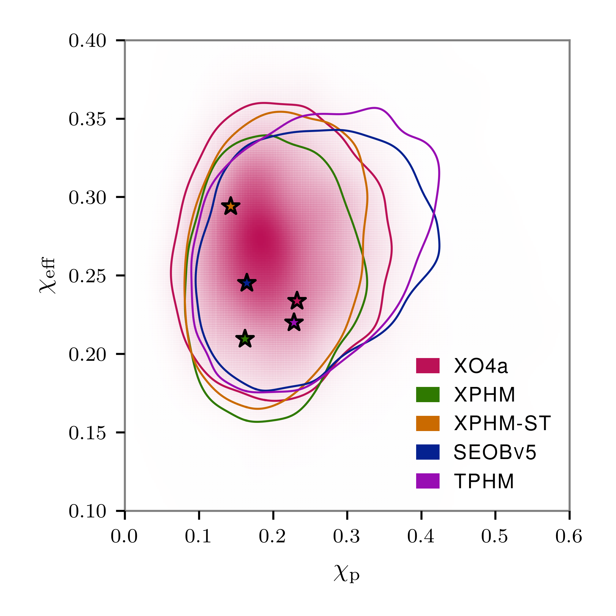
Figure 16: The two-dimensional marginalized posterior distributions for the effective precessing and aligned spin, $\chi_{\mathrm{p}}$ and $\chi_{\mathrm{eff}}$ respectively, when analyzing GW190412. The indicated two-dimensional area shows the inferred 90% credible region and the markers show the maximum likelihood position. The shaded region indicates the posterior probability density per pixel obtained with XO4a.

To analyze GW190412, we use the strain data released by the Gravitational Wave Open Science Center (GWOSC) Abbott et al. (2021c) and the publicly released power spectral densities and calibration envelopes included in the GWTC-2.1 data release Abbott et al. (2021b); Collaboration and Collaboration (2022). Although the original LIGO-Virgo-KAGRA analysis employed a highly parallelized version of Bilby Smith et al. (2020), we use the standard configuration, as described above. All settings were chosen to match the original LIGO-Virgo-KAGRA analysis.

In Fig 16 we show the inferred two-dimensional marginalized posterior distribution for the effective precessing and aligned spin, $\chi_{\mathrm{p}}$ and $\chi_{\mathrm{eff}}$ respectively. We see that although SEOBv5 and TPHM recover a marginally tighter posterior for $\chi_{\mathrm{eff}}$ with slightly more support for larger $\chi_{\mathrm{p}}$, in general all models show excellent agreement for the bulk of the posterior. When comparing maximum likelihood samples, we see that all models approximately agree, but we note that XO4a and TPHM prefer more precession, $\chi_{\mathrm{p}}\sim 0.23$ compared to other models $\chi_{\mathrm{p}}\sim 0.15$, and XPHM with the Spin Taylor precession angles prefers larger aligned spins. Importantly, the two-dimensional 90% contours contain the maximum likelihood samples for all models.

In a typical GW Bayesian analysis, the likelihood is evaluated $\sim 10^{7}$ times. Having a waveform model that not only accurately describes the GW emitted from a binary merger, but also quick to evaluate, is therefore crucial for GW analyses. We find that the full XO4a waveform can be faster to evaluate close to equal mass, and takes longer to evaluate at highly asymmetric masses where the period of two-spin oscillations becomes more comparable to the orbital period. At worst the waveform generation is a factor of $\sim\!2$ slower than XPHM. To check likelihood evaluation time we randomly drew $10^{6}$ points from a standard prior distribution and evaluated the likelihood for each point. We find that on average XO4a is $1.6\times$ and $1.2\times$ slower than XPHM and XPHM with the Spin Taylor precession angles respectively, $8.3\times$ faster than SEOBv5 and $3.4\times$ faster than TPHM. More information about waveform timing is available from the authors upon request.

VI Conclusions

To date, analytic or semi-analytic binary-black-hole waveform models available for analysis of LVK observations have not included any input from fully general-relativistic results (i.e., NR simulations) for precession effects through the merger and ringdown, or the antisymmetric contribution to the signal multipoles. A model that included NR tuning for the dominant symmetric $\ell=2$ contribution, PNR, was presented in Paper I ​. For this model to be used in analysis of real GW signals, it would ideally be extended to include sub-dominant multipoles. In lieu of a full NR tuning to the higher multipoles, the purpose of this work was to incorporate the precision dominant-multipole modeling of PNR into a state-of-the-art higher-multipole model infrastructure, XPHM, and to apply an approximate extension of the merger-ringdown precession dynamics to higher multipoles, and include a model for the antisymmetric contribution Ghosh et al. (2023), to make a series of recent advances in precession modeling Hamilton et al. (2021, 2023b); Ghosh et al. (2023) available for GW signal analysis.

In this first extension of the PNR approach to higher multipoles, we have not performed additional tuning to the higher multipoles, but have instead applied an approximate extension of the (2,2) results by (1) applying a model of the effective ringdown frequency to the coprecessing-frame higher multipoles, as described in Ref. Hamilton et al. (2023b) and Sec. III.1.2, and (2) extending the frequency-domain precession angles for the higher multpoles beyond the SPA prescription used in earlier models, to apply a frequency shift (rather than scaling) through the merger and ringdown, as described in Sec. IV.4. In addition, we have incorporated a model of the antisymmetric contribution to the coprecessing-frame (2,2) multipoles, as described in Ref. Ghosh et al. (2023) and Sec. III.2. We have also made several improvements to the tuning of the precession angles, and, given the smooth behavior of the PNR model across the tuning parameter space, have retuned the model to use both the 40 calibration waveforms used in the original PNR model, plus an additional 40 waveforms that were previously used for validation; all NR waveforms are publicly available and discussed in Ref. Hamilton et al. (2023a).

As in the original PNR model, we find a significant improvement in accuracy over all other models, if we consider only the symmetric (2,2) contribution to the coprecessing frame. If we also consider the antisymmetric contribution in the coprecessing frame then, as we might expect, the accuracy of all symmetric models degrades. Our inclusion of a model for the antisymmetric contribution restores much of the accuracy.

For the full precessing model, the accuracy is limited by the higher multipoles, and we find that the overall accuracy of all of the state-of-the-art models that we consider is comparable; in some measures XO4a does slightly better than others (the NR comparison in Fig. 9, which extends up to $q=8$), while in other measures the SEOBv5 model is more accurate (e.g., mismatch histograms as shown in Figs. 11). We expect that the most significant error in the XO4a higher multipoles is in the relative time and phase offsets between the different multipoles, which we have not explicitly checked or modeled. This may be a problem common to all frequency-domain models, since we find in parameter-estimation tests that the time-domain models SEOBv5 and TPHM show less parameter bias, despite including no precession tuning through merger and ringdown, and (in the case of TPHM) no clear advantage in mismatch comparisons.

As noted in Sec. II, some of the advantages of the “twist-up” procedure of modeling precessing-binary signals are lost when we move beyond the dominant multipole in the frequency domain. If we consider the frequency-domain multipoles in the QA frame, these will neither approximate those from a non-precesing binary in the inspiral, nor exhibit the simple structure of non-precessing-binary multipoles. Convsersely, if we wish to use non-precessing-binary multipoles in the coprecessing frame (as we do here) then we do not have a well-defined prescription for the precession angles. In this work we have been guided by the precession angles we calculate from considering only the $\ell=2$ multipoles, then the $\ell=3$ multipoles, and so on. We do not have a procedure to determine the “correct” angles, against which we could check our model. In future one must either find a way around these issues in order to produce accurate frequency-domain models.

Assuming that there is a way to move beyond these fundamental issues in frequency-domain modeling, XO4a needs to be improved in several ways: we need to model two-spin effects and the relative time and phase shifts between the higher multipoles. We also see that even the symmetric (2,2) coprecessing-frame modeling needs to be improved for configurations with high mass ratios and high spins. As noted in Paper I ​, besides potential improvements in the ansätze to model the precession angles, one may also need to introduce an intermediate frequency region (and make use of longer NR waveforms), and model the evolution of the direction of $\hat{\mathbf{J}}$.

If we look more generally at the suite of state-of-the-art waveform models, we are less concerned with which is most accurate; the differences in accuracy vary significantly across the parameter space, and no model is significantly and consistently more accurate than any other. Of far more interest is that none are sufficiently accurate for upcoming observations. If we make the conservative accuracy requirement that the mismatch must be lower than $\sim$$1/\rho^{2}$ for an SNR of $\rho$ Baird et al. (2013), then at $\rho=30$ we require a mismatch accuracy below $\sim$$10^{-3}$, and at $\rho=40$ we require mismatch uncertainties below $\sim$$10^{-4}$. This is a conservative estimate, but given that the typical mismatch uncertainty is above $10^{-3}$ for all precessing-binary models, a dramatic increase in accuracy is needed. The possible exceptions are the NR surrogate models, but these are currently limited to high-mass binaries. As such it is possible that systematic errors due to model innacuracy will be an issue for the loudest (and therefore most interesting) signals in O4, and almost certainly in future observing runs, unless there is a significant (i.e., order of magnitude) increase in overall accuracy of the state-of-the-art models.

We also require a more complete understanding of the uncertainties in NR waveforms, both as input to models as for validation, and a more robust methods to quantify the impact of model uncertainties on parameter measurements. It is well known that the indistinguishability SNR is a conservative measure of waveform accuracy, and this is illustrated in Sec. V.5, where we see that mismatch error of each model at the true parameters does not reflect the relative performance of each model in parameter recovery. Given that model accuracy is likely to be an important issue for the most interesting observations, there is an urgent need for better methods to quantify the measurement uncertainties that will result from modelling errors.

VII Acknowledgements

We the authors of this work would like to thank Angela Borschers, Rossella Gamba, Cecilio García-Quirós, Lucy Thomas, and Frank Ohme for their tireless efforts and assistance during the IMRPhenomXO4a code review, and Tousif Islam for insighful comments about the manuscript. We also express thanks to Antoni Ramos-Buades , Héctor Estellés, and Cecilio García-Quirós for their guidance in utilizing pySEOBNR.

JT, SG, PK, CH and MH were supported in part by Science and Technology Facilities Council (STFC) grant ST/V00154X/1 and European Research Council (ERC) Consolidator Grant 647839. JT also acknowledges support from the NASA LISA Preparatory Science grant 20-LPS20-0005. EH was supported in part by Swiss National Science Foundation (SNSF) grant IZCOZ0-189876 and by the UZH Postdoc Grant (Forschungskredit). LL was supported at King’s College London by Royal Society University Research Grant URF\R1\211451; and at the University of Amsterdam by the GRAPPA Prize. SG was also supported from the Max Planck Society’s Independent Research Group program. PK was also supported by the GW consolidated grant: STFC grant ST/V005677/1. CH thanks the UKRI Future Leaders Fellowship for support through the grant MR/T01881X/1. EH was also supported in part by the Universitat de les Illes Balears (UIB); the Spanish Agencia Estatal de Investigación grants PID2022-138626NB-I00, PID2019-106416GB-I00, RED2022-134204-E, RED2022-134411-T, funded by MCIN/AEI/10.13039/501100011033; the MCIN with funding from the European Union NextGenerationEU/PRTR (PRTR-C17.I1); Comunitat Autonòma de les Illes Balears through the Direcció General de Recerca, Innovació I Transformació Digital with funds from the Tourist Stay Tax Law (PDR2020/11 - ITS2017-006), the Conselleria d’Economia, Hisenda i Innovació grant numbers SINCO2022/18146 and SINCO2022/6719, co-financed by the European Union and FEDER Operational Program 2021-2027 of the Balearic Islands; the “ERDF A way of making Europe”.

The catalogue of numerical simulations against which this model was calibrated were performed on the DiRAC@Durham facility, managed by the Institute for Computational Cosmology on behalf of the STFC DiRAC HPC Facility (www.dirac.ac.uk). The equipment was funded by BEIS capital funding via STFC capital grants ST/P002293/1 and ST/R002371/1, Durham University and STFC operations grant ST/R000832/1. In addition, several of the simulations used in this work were performed as part of an allocation graciously provided by Oracle to explore the use of our code on the Oracle Cloud Infrastructure.

The authors are additionally grateful for computational resources provided by the LIGO laboratory and supported by National Science Foundation Grants PHY-0757058 and PHY-0823459, which were used to perform the match comparisons presented in this paper.

Most parameter estimation analyses were performed on the Sciama High Performance Compute (HPC) cluster, which is supported by the ICG, SEPNet and the University of Portsmouth. Additional parameter estimation and further analyses were performed on the supercomputing facilities at Cardiff University operated by Advanced Research Computing at Cardiff (ARCCA) on behalf of the Cardiff Supercomputing Facility and the HPC Wales and Supercomputing Wales (SCW) projects. We acknowledge the support of the latter, which is part-funded by the European Regional Development Fund (ERDF) via the Welsh Government. In part the computational resources at Cardiff University were also supported by STFC grant ST/I006285/1.

This research has made use of data or software obtained from the Gravitational Wave Open Science Center (gwosc.org), a service of the LIGO Scientific Collaboration, the Virgo Collaboration, and KAGRA. This material is based upon work supported by NSF’s LIGO Laboratory which is a major facility fully funded by the National Science Foundation, as well as the Science and Technology Facilities Council (STFC) of the United Kingdom, the Max-Planck-Society (MPS), and the State of Niedersachsen/Germany for support of the construction of Advanced LIGO and construction and operation of the GEO600 detector. Additional support for Advanced LIGO was provided by the Australian Research Council. Virgo is funded, through the European Gravitational Observatory (EGO), by the French Centre National de Recherche Scientifique (CNRS), the Italian Istituto Nazionale di Fisica Nucleare (INFN) and the Dutch Nikhef, with contributions by institutions from Belgium, Germany, Greece, Hungary, Ireland, Japan, Monaco, Poland, Portugal, Spain. KAGRA is supported by Ministry of Education, Culture, Sports, Science and Technology (MEXT), Japan Society for the Promotion of Science (JSPS) in Japan; National Research Foundation (NRF) and Ministry of Science and ICT (MSIT) in Korea; Academia Sinica (AS) and National Science and Technology Council (NSTC) in Taiwan.

Appendix A LALSuite Waveform Implementation

In this section we provide a brief description of the waveform parameters available for using in XO4a and the locations of the specific fit coefficients mentioned throughout the text.

In Table 2 we present the tuning parameters for the coprecessing tuning outlined in Sec. III.1.1 and listed in Eq. (4). These variables are presented alongside their names in the LAL code and the associated XAS parameter they modify. The final values of these fit coefficients are available within the file LALSimIMRPhenomX_PNR_deviations.c in LALSuite LIGO Scientific Collaboration (2018).

$u_{k}$	Name in LAL code	XAS parameter ($\lambda_{k}$)
$u_{0}$	MU1	pAmp->v1RD
$u_{1}$	MU2	pAmp->gamma3
$u_{2}$	MU3	V2
$u_{5}$	NU4	pPhase->cL
$u_{6}$	NU5	pWF->fRING
$u_{7}$	NU6	pWF->fDAMP
$u_{8}$	ZETA1	pPhase->b4
$u_{9}$	ZETA2	pPhase->b1

Table 2: Deviation variables for tuning of the $(\ell,|m|)=(2,2)$ multipole moment: Changes are made within LALSimIMRPhenomX_internals.c and LALSimIMRPhenomX_precession.c at or shortly after the definition of related structure parameters.

The fit coefficients for the tuned precession angles discussed in Sec. IV.1.1, along with the fit coefficients for the $\beta_{\text{f}}$ fit detailed in Sec. IV.2, may be found in the file LALSimIMRPhenomX_PNR_coefficients.c in LALSuite. All results in this paper were produced with the coefficients found in the git hash: 08b90494b3a4a7dc966ca108e6c98eaa3f6e18a7.

In Table 3 we show the available waveform parameter flags used to modify the behavior of IMRPhenomXO4a present in LALSimulation, along with a description of the behavior that each parameter controls. One should note that, at present, enabling PhenomXAntisymmetricWaveform also requires enabling PhenomXPNRUseTunedAngles for the antisymmetric contributions to be present, otherwise an error is raised upon waveform generation.

Parameter name in LAL code	Description	Values	Default
PhenomXPNRUseTunedAngles	Enables tuned precession angles in XPHM framework.	0,1	0
PhenomXPNRUseTunedCoprec	Enables tuned $(\ell,m)=(2,2)$ coprecessing model in XPHM framework.	0,1	0
PhenomXPNRInterpTolerance	Sets the interpolation residual error threshold $R$ detailed in Eq. (57).	Float	0.01
PhenomXAntisymmetricWaveform	Enables the antisymmetric contribution to the $(\ell,m)=(2,\pm 2)$ coprecessing multipole.	0,1	0

Table 3: The available waveform parameters added to XPHM to activate the various contributions that make up the XO4a model, coded in LALSimulation as IMRPhenomXO4a. Currently PhenomXAntisymmetricWaveform only activates when the flag is enabled and PhenomXPNRUseTunedAngles is also activated.

References

- Abbott et al. (2018) B. P. Abbott et al. (KAGRA, LIGO Scientific, Virgo, VIRGO), Living Rev. Rel. 21, 3 (2018), arXiv:1304.0670 [gr-qc] .
- Aasi et al. (2015) J. Aasi et al. (LIGO Scientific), Class. Quant. Grav. 32, 074001 (2015), arXiv:1411.4547 [gr-qc] .
- Acernese et al. (2015) F. Acernese et al. (VIRGO), Class. Quant. Grav. 32, 024001 (2015), arXiv:1408.3978 [gr-qc] .
- Akutsu et al. (2021) T. Akutsu et al. (KAGRA), PTEP 2021, 05A101 (2021), arXiv:2005.05574 [physics.ins-det] .
- Abbott et al. (2019) B. P. Abbott et al. (LIGO Scientific, Virgo), Phys. Rev. X 9, 031040 (2019), arXiv:1811.12907 [astro-ph.HE] .
- Abbott et al. (2021a) R. Abbott et al. (LIGO Scientific, Virgo), Phys. Rev. X 11, 021053 (2021a), arXiv:2010.14527 [gr-qc] .
- Abbott et al. (2021b) R. Abbott et al. (LIGO Scientific, VIRGO), (2021b), arXiv:2108.01045 [gr-qc] .
- Abbott et al. (2023a) R. Abbott et al. (LIGO Scientific Collaboration, Virgo Collaboration, and KAGRA Collaboration), Phys. Rev. X 13, 041039 (2023a), arXiv:2111.03606 [gr-qc] .
- Nitz et al. (2023) A. H. Nitz, S. Kumar, Y.-F. Wang, S. Kastha, S. Wu, M. Schäfer, R. Dhurkunde, and C. D. Capano, Astrophys. J. 946, 59 (2023), arXiv:2112.06878 [astro-ph.HE] .
- Venumadhav et al. (2020) T. Venumadhav, B. Zackay, J. Roulet, L. Dai, and M. Zaldarriaga, Phys. Rev. D 101, 083030 (2020), arXiv:1904.07214 [astro-ph.HE] .
- Mehta et al. (2023) A. K. Mehta, S. Olsen, D. Wadekar, J. Roulet, T. Venumadhav, J. Mushkin, B. Zackay, and M. Zaldarriaga, (2023), arXiv:2311.06061 [gr-qc] .
- Husa et al. (2016) S. Husa, S. Khan, M. Hannam, M. Pürrer, F. Ohme, X. Jiménez Forteza, and A. Bohé, Phys. Rev. D 93, 044006 (2016), arXiv:1508.07250 [gr-qc] .
- Khan et al. (2016) S. Khan, S. Husa, M. Hannam, F. Ohme, M. Pürrer, X. Jiménez Forteza, and A. Bohé, Phys. Rev. D 93, 044007 (2016), arXiv:1508.07253 [gr-qc] .
- Hannam et al. (2014) M. Hannam, P. Schmidt, A. Bohé, L. Haegel, S. Husa, F. Ohme, G. Pratten, and M. Pürrer, Phys. Rev. Lett. 113, 151101 (2014), arXiv:1308.3271 [gr-qc] .
- London et al. (2018) L. London, S. Khan, E. Fauchon-Jones, C. García, M. Hannam, S. Husa, X. Jiménez-Forteza, C. Kalaghatgi, F. Ohme, and F. Pannarale, Phys. Rev. Lett. 120, 161102 (2018), arXiv:1708.00404 [gr-qc] .
- Dietrich et al. (2019) T. Dietrich, A. Samajdar, S. Khan, N. K. Johnson-McDaniel, R. Dudi, and W. Tichy, Phys. Rev. D 100, 044003 (2019), arXiv:1905.06011 [gr-qc] .
- Khan et al. (2020) S. Khan, F. Ohme, K. Chatziioannou, and M. Hannam, Phys. Rev. D 101, 024056 (2020), arXiv:1911.06050 [gr-qc] .
- Thompson et al. (2020) J. E. Thompson, E. Fauchon-Jones, S. Khan, E. Nitoglia, F. Pannarale, T. Dietrich, and M. Hannam, Phys. Rev. D 101, 124059 (2020), arXiv:2002.08383 [gr-qc] .
- Pratten et al. (2020) G. Pratten, S. Husa, C. Garcia-Quiros, M. Colleoni, A. Ramos-Buades, H. Estelles, and R. Jaume, Phys. Rev. D 102, 064001 (2020), arXiv:2001.11412 [gr-qc] .
- García-Quirós et al. (2020) C. García-Quirós, M. Colleoni, S. Husa, H. Estellés, G. Pratten, A. Ramos-Buades, M. Mateu-Lucena, and R. Jaume, Phys. Rev. D 102, 064002 (2020), arXiv:2001.10914 [gr-qc] .
- Pratten et al. (2021) G. Pratten et al., Phys. Rev. D 103, 104056 (2021), arXiv:2004.06503 [gr-qc] .
- Estellés et al. (2022) H. Estellés, M. Colleoni, C. García-Quirós, S. Husa, D. Keitel, M. Mateu-Lucena, M. d. L. Planas, and A. Ramos-Buades, Phys. Rev. D 105, 084040 (2022), arXiv:2105.05872 [gr-qc] .
- Taracchini et al. (2014) A. Taracchini et al., Phys. Rev. D 89, 061502 (2014), arXiv:1311.2544 [gr-qc] .
- Pan et al. (2014) Y. Pan, A. Buonanno, A. Taracchini, L. E. Kidder, A. H. Mroué, H. P. Pfeiffer, M. A. Scheel, and B. Szilágyi, Phys. Rev. D 89, 084006 (2014), arXiv:1307.6232 [gr-qc] .
- Cotesta et al. (2018) R. Cotesta, A. Buonanno, A. Bohé, A. Taracchini, I. Hinder, and S. Ossokine, Phys. Rev. D 98, 084028 (2018), arXiv:1803.10701 [gr-qc] .
- Ossokine et al. (2020) S. Ossokine et al., Phys. Rev. D 102, 044055 (2020), arXiv:2004.09442 [gr-qc] .
- Matas et al. (2020) A. Matas et al., Phys. Rev. D 102, 043023 (2020), arXiv:2004.10001 [gr-qc] .
- Pompili et al. (2023) L. Pompili et al., (2023), arXiv:2303.18039 [gr-qc] .
- Ramos-Buades et al. (2023) A. Ramos-Buades, A. Buonanno, H. Estellés, M. Khalil, D. P. Mihaylov, S. Ossokine, L. Pompili, and M. Shiferaw, (2023), arXiv:2303.18046 [gr-qc] .
- Blackman et al. (2017) J. Blackman, S. E. Field, M. A. Scheel, C. R. Galley, D. A. Hemberger, P. Schmidt, and R. Smith, Phys. Rev. D 95, 104023 (2017), arXiv:1701.00550 [gr-qc] .
- Varma et al. (2019a) V. Varma, S. E. Field, M. A. Scheel, J. Blackman, L. E. Kidder, and H. P. Pfeiffer, Phys. Rev. D 99, 064045 (2019a), arXiv:1812.07865 [gr-qc] .
- Varma et al. (2019b) V. Varma, S. E. Field, M. A. Scheel, J. Blackman, D. Gerosa, L. C. Stein, L. E. Kidder, and H. P. Pfeiffer, Phys. Rev. Research. 1, 033015 (2019b), arXiv:1905.09300 [gr-qc] .
- Islam et al. (2021a) T. Islam, V. Varma, J. Lodman, S. E. Field, G. Khanna, M. A. Scheel, H. P. Pfeiffer, D. Gerosa, and L. E. Kidder, Phys. Rev. D 103, 064022 (2021a), arXiv:2101.11798 [gr-qc] .
- Hamilton et al. (2021) E. Hamilton, L. London, J. E. Thompson, E. Fauchon-Jones, M. Hannam, C. Kalaghatgi, S. Khan, F. Pannarale, and A. Vano-Vinuales, Phys. Rev. D 104, 124027 (2021), arXiv:2107.08876 [gr-qc] .
- Hamilton et al. (2023a) E. Hamilton, E. Fauchon-Jones, M. Hannam, C. Hoy, C. Kalaghatgi, L. London, J. E. Thompson, D. Yeeles, S. Ghosh, S. Khan, P. Kolitsidou, and A. Vano-Vinuales, (2023a), arXiv:2303.05419 [gr-qc] .
- Hamilton et al. (2023b) E. Hamilton, L. London, and M. Hannam, Phys. Rev. D 107, 104035 (2023b), arXiv:2301.06558 [gr-qc] .
- Ghosh et al. (2023) S. Ghosh, P. Kolitsidou, and M. Hannam, (2023), arXiv:2310.16980 [gr-qc] .
- Schmidt et al. (2012) P. Schmidt, M. Hannam, and S. Husa, Phys. Rev. D 86, 104063 (2012), arXiv:1207.3088 [gr-qc] .
- Khan et al. (2019) S. Khan, K. Chatziioannou, M. Hannam, and F. Ohme, Phys. Rev. D 100, 024059 (2019), arXiv:1809.10113 [gr-qc] .
- Chatziioannou et al. (2017) K. Chatziioannou, A. Klein, N. Cornish, and N. Yunes, Phys. Rev. Lett. 118, 051101 (2017), arXiv:1606.03117 [gr-qc] .
- Colleoni et al. (2024) M. Colleoni et al., (2024), in preparation.
- Yu et al. (2023) H. Yu, J. Roulet, T. Venumadhav, B. Zackay, and M. Zaldarriaga, Phys. Rev. D 108, 064059 (2023), arXiv:2306.08774 [gr-qc] .
- Ajith et al. (2011) P. Ajith et al., Phys. Rev. Lett. 106, 241101 (2011), arXiv:0909.2867 [gr-qc] .
- Santamaria et al. (2010) L. Santamaria et al., Phys. Rev. D 82, 064016 (2010), arXiv:1005.3306 [gr-qc] .
- Schmidt et al. (2015) P. Schmidt, F. Ohme, and M. Hannam, Phys. Rev. D 91, 024043 (2015), arXiv:1408.1810 [gr-qc] .
- LIGO Scientific Collaboration (2018) LIGO Scientific Collaboration, “LIGO Algorithm Library - LALSuite,” free software (GPL) (2018).
- Wette (2020) K. Wette, SoftwareX 12, 100634 (2020).
- Schmidt et al. (2011) P. Schmidt, M. Hannam, S. Husa, and P. Ajith, Phys. Rev. D 84, 024046 (2011), arXiv:1012.2879 [gr-qc] .
- Pekowsky et al. (2013) L. Pekowsky, R. O’Shaughnessy, J. Healy, and D. Shoemaker, Phys. Rev. D 88, 024040 (2013), arXiv:1304.3176 [gr-qc] .
- Ramos-Buades et al. (2020) A. Ramos-Buades, P. Schmidt, G. Pratten, and S. Husa, Phys. Rev. D 101, 103014 (2020), arXiv:2001.10936 [gr-qc] .
- O’Shaughnessy et al. (2011) R. O’Shaughnessy, B. Vaishnav, J. Healy, Z. Meeks, and D. Shoemaker, Phys. Rev. D 84, 124002 (2011), arXiv:1109.5224 [gr-qc] .
- Boyle et al. (2011) M. Boyle, R. Owen, and H. P. Pfeiffer, Phys. Rev. D 84, 124011 (2011), arXiv:1110.2965 [gr-qc] .
- London and Fauchon-Jones (2019) L. London and E. Fauchon-Jones, Class. Quant. Grav. 36, 235015 (2019), arXiv:1810.03550 [gr-qc] .
- Jiménez-Forteza et al. (2017) X. Jiménez-Forteza, D. Keitel, S. Husa, M. Hannam, S. Khan, and M. Pürrer, Phys. Rev. D 95, 064024 (2017), arXiv:1611.00332 [gr-qc] .
- Arun et al. (2009) K. G. Arun, A. Buonanno, G. Faye, and E. Ochsner, Phys. Rev. D 79, 104023 (2009), [Erratum: Phys.Rev.D 84, 049901 (2011)], arXiv:0810.5336 [gr-qc] .
- Boyle et al. (2014) M. Boyle, L. E. Kidder, S. Ossokine, and H. P. Pfeiffer, (2014), arXiv:1409.4431 [gr-qc] .
- Kalaghatgi and Hannam (2021) C. Kalaghatgi and M. Hannam, Phys. Rev. D 103, 024024 (2021), arXiv:2008.09957 [gr-qc] .
- Bruegmann et al. (2008) B. Bruegmann, J. A. Gonzalez, M. Hannam, S. Husa, and U. Sperhake, Phys. Rev. D 77, 124047 (2008), arXiv:0707.0135 [gr-qc] .
- Kolitsidou et al. (2023) P. Kolitsidou, J. E. Thompson, and M. Hannam, (2023), in preparation.
- Hannam et al. (2022) M. Hannam et al., Nature 610, 652 (2022), arXiv:2112.11300 [gr-qc] .
- Varma et al. (2022) V. Varma, S. Biscoveanu, T. Islam, F. H. Shaik, C.-J. Haster, M. Isi, W. M. Farr, S. E. Field, and S. Vitale, Phys. Rev. Lett. 128, 191102 (2022), arXiv:2201.01302 [astro-ph.HE] .
- Chatziioannou et al. (2017) K. Chatziioannou, A. Klein, N. Yunes, and N. Cornish, Phys. Rev. D 95, 104004 (2017), arXiv:1703.03967 [gr-qc] .
- Bohe et al. (2013) A. Bohe, S. Marsat, G. Faye, and L. Blanchet, Class. Quant. Grav. 30, 075017 (2013), arXiv:1212.5520 [gr-qc] .
- Schmidt et al. (2017) P. Schmidt, I. W. Harry, and H. P. Pfeiffer, (2017), arXiv:1703.01076 [gr-qc] .
- Galassi and Gough (2009) M. Galassi and B. Gough, GNU Scientific Library: Reference Manual, GNU manual (Network Theory, 2009).
- García-Quirós et al. (2021) C. García-Quirós, S. Husa, M. Mateu-Lucena, and A. Borchers, Class. Quant. Grav. 38, 015006 (2021), arXiv:2001.10897 [gr-qc] .
- Hall and Meyer (1976) C. A. Hall and W. Meyer, Journal of Approximation Theory 16, 105 (1976).
- (68) LSC, “LIGO Document T1800044-v5,” https://dcc.ligo.org/LIGO-T1800044/public.
- Veitch et al. (2015) J. Veitch et al., Phys. Rev. D 91, 042003 (2015), arXiv:1409.7215 [gr-qc] .
- Allen et al. (2012) B. Allen, W. G. Anderson, P. R. Brady, D. A. Brown, and J. D. E. Creighton, Phys. Rev. D 85, 122006 (2012), arXiv:gr-qc/0509116 .
- Babak et al. (2013) S. Babak et al., Phys. Rev. D 87, 024033 (2013), arXiv:1208.3491 [gr-qc] .
- Baird et al. (2013) E. Baird, S. Fairhurst, M. Hannam, and P. Murphy, Phys. Rev. D 87, 024035 (2013), arXiv:1211.0546 [gr-qc] .
- Acernese et al. (2014) F. Acernese, M. Agathos, K. Agatsuma, D. Aisa, N. Allemandou, A. Allocca, J. Amarni, P. Astone, G. Balestri, G. Ballardin, et al., Classical and Quantum Gravity 32, 024001 (2014).
- Speagle (2020) J. S. Speagle, Mon. Not. Roy. Astron. Soc. 493, 3132 (2020), arXiv:1904.02180 [astro-ph.IM] .
- Ashton et al. (2019) G. Ashton et al., Astrophys. J. Suppl. 241, 27 (2019), arXiv:1811.02042 [astro-ph.IM] .
- Romero-Shaw et al. (2020) I. M. Romero-Shaw et al., Mon. Not. Roy. Astron. Soc. 499, 3295 (2020), arXiv:2006.00714 [astro-ph.IM] .
- Cutler and Flanagan (1994) C. Cutler and E. E. Flanagan, Phys. Rev. D 49, 2658 (1994), arXiv:gr-qc/9402014 .
- Poisson and Will (1995) E. Poisson and C. M. Will, Phys. Rev. D 52, 848 (1995), arXiv:gr-qc/9502040 .
- Hoy (2022) C. Hoy, Phys. Rev. D 106, 083003 (2022), arXiv:2208.00106 [gr-qc] .
- Abbott et al. (2023b) R. Abbott et al. (KAGRA, VIRGO, LIGO Scientific), Phys. Rev. X 13, 011048 (2023b), arXiv:2111.03634 [astro-ph.HE] .
- Abbott et al. (2016a) B. P. Abbott et al. (LIGO Scientific, Virgo), Phys. Rev. Lett. 116, 061102 (2016a), arXiv:1602.03837 [gr-qc] .
- Abbott et al. (2016b) B. P. Abbott et al. (LIGO Scientific, Virgo), Phys. Rev. Lett. 116, 241102 (2016b), arXiv:1602.03840 [gr-qc] .
- Abbott et al. (2020a) R. Abbott et al. (LIGO Scientific, Virgo), Phys. Rev. D 102, 043015 (2020a), arXiv:2004.08342 [astro-ph.HE] .
- Abbott et al. (2020b) R. Abbott et al. (LIGO Scientific, Virgo), Astrophys. J. Lett. 896, L44 (2020b), arXiv:2006.12611 [astro-ph.HE] .
- Colleoni et al. (2021) M. Colleoni, M. Mateu-Lucena, H. Estellés, C. García-Quirós, D. Keitel, G. Pratten, A. Ramos-Buades, and S. Husa, Phys. Rev. D 103, 024029 (2021), arXiv:2010.05830 [gr-qc] .
- Islam et al. (2021b) T. Islam, S. E. Field, C.-J. Haster, and R. Smith, Phys. Rev. D 103, 104027 (2021b), arXiv:2010.04848 [gr-qc] .
- Hoy et al. (2022) C. Hoy, C. Mills, and S. Fairhurst, Phys. Rev. D 106, 023019 (2022), arXiv:2111.10455 [gr-qc] .
- Abbott et al. (2021c) R. Abbott et al. (LIGO Scientific, Virgo), SoftwareX 13, 100658 (2021c), arXiv:1912.11716 [gr-qc] .
- Collaboration and Collaboration (2022) L. S. Collaboration and V. Collaboration, “GWTC-2.1: Deep Extended Catalog of Compact Binary Coalescences Observed by LIGO and Virgo During the First Half of the Third Observing Run - Parameter Estimation Data Release,” (2022), LIGO Laboratory and Advanced LIGO are funded by the United States National Science Foundation (NSF) as well as the Science and Technology Facilities Council (STFC) of the United Kingdom, the Max-Planck-Society (MPS), and the State of Niedersachsen/Germany for support of the construction of Advanced LIGO and construction and operation of the GEO600 detector. Additional support for Advanced LIGO was provided by the Australian Research Council. Virgo is funded, through the European Gravitational Observatory (EGO), by the French Centre National de Recherche Scientifique (CNRS), the Italian Istituto Nazionale di Fisica Nucleare (INFN) and the Dutch Nikhef, with contributions by institutions from Belgium, Germany, Greece, Hungary, Ireland, Japan, Monaco, Poland, Portugal, Spain.
- Smith et al. (2020) R. J. E. Smith, G. Ashton, A. Vajpeyi, and C. Talbot, Mon. Not. Roy. Astron. Soc. 498, 4492 (2020), arXiv:1909.11873 [gr-qc] .