$m_{B}$ and $f_{B^{(\star)}}$ in $2+1$ flavour QCD from a combination of continuum limit static and relativistic results

Abstract

We present preliminary results for B-physics from a combination of non-perturbative results in the static limit with relativistic computations satisfying $am_{\mathrm{heavy}}\ll 1$. Relativistic measurements are carried out at the physical b-quark mass using the Schrödinger Functional in a $0.5\ \mathrm{fm}$ box. They are connected to large volume observables through step scaling functions that trace the mass dependence between the physical charm region and the static limit, such that B-physics results can be obtained by interpolation; the procedure is designed to exactly cancel the troublesome $\alpha_{s}(m_{\mathrm{heavy}})^{n+\gamma}$ corrections to large mass scaling. Large volume computations for both static and relativistic quantities use CLS $N_{f}=2+1$ ensembles at $m_{u}=m_{d}=m_{s}$, and with five values of the lattice spacing down to $0.039$ fm. Our preliminary results for the b-quark mass and leptonic decay constants have competitive uncertainties, which are furthermore dominated by statistics, allowing for substantial future improvement. Here we focus on numerical results, while the underlying strategy is discussed in a companion contribution [1].

1 Introduction

Fundamental processes involving heavy quarks are crucial to explore indirect searches of new physics beyond the Standard Model (SM). In this context, a precise non-perturbative determination of B-physics observables is essential to probe new phenomena that may manifest themselves as subtle deviations from the theoretical predictions.

We have further developed a methodology first proposed in [2], where a static computation $m_{h}\to\infty$ was combined with a relativistic one $m_{h}<m_{b}$ in order to reach the physical b-quark scale by interpolation while controlling cutoff effects in each step of the computation. Our approach, detailed in [1], consists in building suitable quantities with a continuum limit and a simple behavior in $1/m_{h}$ in order to perform the interpolation between the two sets of results. The design principle is a complete cancellation of renormalisation and matching factors in the static theory. The latter diverge in the static limit, thus posing serious difficulties to control systematic uncertainties.

Our strategy requires a set of finite volume ensembles, from $L_{1}=2L_{0}\approx 0.5\ \mathrm{fm}$ where we reach the relativistic b-quark scale, to $L_{2}\approx 1.0\ \mathrm{fm}$, where we perform both static and relativistic measurements. We cover a range of heavy quark masses that starts below the charm region and extends up to or above the bottom quark mass, while the light quark masses are set to zero in finite volume. In $L_{2}$, as we double the box size and the lattice spacing, discretisation effects increase significantly above $m_{b}/2$. Eventually we make contact with Nature by connecting to the large volume $SU(3)$ symmetric point $m_{u}=m_{d}=m_{s}$ through CLS ensembles [3, 4, 5, 6]. Different volumes are connected by step scaling [7, 8, 2].

2 b-quark mass

We extract the b-quark mass from the step scaling chain [1]

$$m_{b}^{\mathrm{RGI}}=\frac{1}{L_{\mathrm{ref}}}\frac{y_{B}-\rho_{m}(u_{2},y_{B})-\sigma_{m}(u_{1},y_{2})}{\pi_{m}(u_{1},y_{1})},$$ (1)

where we define the Step Scaling Functions (SSF)

$$\sigma_{m}(u_{1},y_{2})=L_{\mathrm{ref}}[m_{H}(L_{2})-m_{H}(L_{1})],\qquad\rho_{m}(u_{1},y_{2})=L_{\mathrm{ref}}[m_{B}-m_{H}(L_{2})],$$ (2)

made dimensionless in units of a length-scale $L_{\mathrm{ref}}$. We specify the different volumes of size $L_{i}^{4}$ in terms of the running couplings $u_{i}=\bar{g}^{2}(L_{i})$ of [9, 10],

$$u_{0}=3.949,\;u_{1}=5.862(27),\;u_{2}=11.252(83)\,,$$ (3)

while the heavy-light meson masses $y_{i}=L_{\mathrm{ref}}m_{H}(L_{i})$ in units of $L_{\mathrm{ref}}$ are used as proxies for the b-quark mass. They are determined recursively from the large volume physical input according to

$$y_{B}\equiv L_{\mathrm{ref}}m_{\overline{B}},\qquad y_{2}=y_{B}-\rho_{m}(u_{2},y_{B}),\qquad y_{1}=y_{2}-\sigma_{m}(u_{1},y_{2}),$$ (4)

where $m_{\overline{B}}=\frac{2}{3}m_{B}+\frac{1}{3}m_{B_{s}}=5308.5(2)\ \mathrm{MeV}$ denotes the flavour averaged combination of $B$ and $B_{s}$ meson masses [11] used to fix the physical b-quark mass. This is the natural choice at the symmetric point ($M_{\pi}=M_{K}\approx 415\ \mathrm{MeV}$ [12]). Finally, $\pi_{m}(u_{1},y_{1})$ in Eq. (2) is the ratio

$$\pi_{m}(u_{1},y_{1})=\frac{m_{H}(L_{1})}{m_{b}^{\mathrm{RGI}}}=\frac{y_{1}}{L_{\mathrm{ref}}m_{b}^{\mathrm{RGI}}},$$ (5)

used to convert pseudo-scalar masses to RGI quark masses,

$$m_{h}^{\mathrm{RGI}}=h(L_{0})\frac{Z(g_{0}^{2})Z_{A}(g_{0}^{2})}{Z_{P}(g_{0}^{2},L_{0})}(1+b_{m}(g_{0}^{2})am_{q,h})m_{q,h},$$ (6)

with $m_{q,h}$ the bare subtracted quark mass. The renormalisation constants $Z_{A}$, $Z_{P}$, $Z$ and $b_{m}$ have been determined specifically for our bare coupling range [10, 13], while the non-perturbative RG running factor $h(L_{0})=1.4744(85)$ has been computed using the results of [14].

We now move to the numerical results for the SSFs. In our practical implementation we set $L_{\mathrm{ref}}=4L_{0}=L_{2}$.

2.1 $L_{2}$ to $L_{\mathrm{CLS}}$ step scaling functions

This first step connects the finite volume $L_{2}$ with vanishing sea quark masses to the large volume CLS ensembles at the symmetric point. Bare couplings were tuned such that $\bar{g}^{2}(L_{2})=11.27$ (a preliminary value at the start of the project) within a sufficient precision $\Delta\bar{g}^{2}=0.1$ for $L_{2}/a=12,\ldots,32$. This results in $\beta\in[3.4,3.97]$ overlapping well with CLS ensembles. Short interpolations of $L/a=f(\tilde{g}_{0}^{2})$ to the CLS improved bare parameters $\tilde{g}_{0}^{2}$ (see [15, 16] for the definition) are required to match the two sets of data. Next finite volume and infinite volume heavy-light pseudo-scalar masses are computed at a suitably chosen set of bare heavy quark masses $a\tilde{m}_{\mathrm{q},h}$. For each (non-integer) resolution $a/L$ all heavy-light quantities are then interpolated to common improved bare parameters $\tilde{g}_{0}^{2},a\tilde{m}_{\mathrm{q},i}$ and these are interpolated again to a set of $\{y^{\mathrm{targ}}\}$ (defined in large volume). For each $y^{\mathrm{targ}}$ we then have finite volume and infinite volume masses for the same improved bare parameters at each resolution $a/L_{2}$.

This yields the relativistic SSFs at finite lattice spacing,

$$R_{m}(u_{2},y^{\mathrm{targ}},a/L_{2})=L_{2}[(m_{H})_{\mathcal{S}_{m}}-(m(L_{2}))_{\mathcal{S}_{0}}]\,.$$ (7)

The static ones are obtained in the same way but do not need an interpolation to a fixed $y^{\mathrm{targ}}$. Here $\mathcal{S}_{0}$ and $\mathcal{S}_{m}$ denote the massless and massive Lines of Constant Physics (LCP) defined in [1] and connected by the common improved bare coupling $\tilde{g}_{0}^{2}$ as just explained.

The extrapolation to $\rho(u,y)=R_{m}(u,y,0)$ is performed with the fit ansatz

$$R_{m}=p_{0}+p_{1}(a/L_{2})^{2},\qquad R_{m}^{\mathrm{stat}}=s_{0}+s_{1}(a/L_{2})^{2}.$$ (8)

Cutoff effects are compatible with a linear dependence on $a^{2}$, cf. Fig. 1. For the relativistic $R_{m}(u_{2},y^{\mathrm{targ}}_{i},a/L_{2})$ we include only data with $am_{h}^{\mathrm{RGI}}<0.8$ in the fit and in the static theory we drop the two coarsest lattice spacings. The improvement coefficient $c_{A}^{\mathrm{stat}}$ is needed for O($a$) improvement of $R_{m}^{\mathrm{stat}}$. However, $c_{A}^{\mathrm{stat}}$ is not yet known for the Lüscher-Weisz gauge action. We currently estimate it by the 1-loop $c_{A}^{\mathrm{stat}}$ of the Wilson gauge action [17] and assign a $200\%$ error.

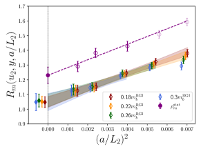
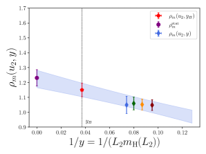
Figure 1: Left: continuum limit extrapolation for the relativistic (diamonds) and static (circles) SSF connecting the volume $L_{2}\to\mathrm{CLS}$. Right: interpolation between the static and relativistic continuum SSF to the target b-quark scale $y_{B}$.

We then interpolate the continuum results for $\rho_{m}(u_{2},y^{\mathrm{targ}})$ and $\rho_{m}^{\mathrm{stat}}(u_{2})$ to the physical point $y=y_{B}=26.87(18)$ through the functional form

$$\rho_{m}=t_{0}+t_{1}y^{-1}+t_{2}y^{-2},$$ (9)

where $t_{i}$ are fit parameters. The interpolation is shown on the right plot of Fig. 1. In this case, the quadratic term is not needed in the fit and we set $t_{2}=0$. At the physical point we deduce

$$\rho_{m}(u_{2},y_{B})=1.152(45)\,,\quad\to\quad y_{2}=25.72(19).$$ (10)

2.2 $L_{1}$ to $2L_{1}$ step scaling functions

In the second step of the computation we determine the SSF $\sigma_{m}(u_{1},y_{2})$ connecting the finite volumes $L_{1}$ and $L_{2}=2L_{1}$, generated at common values of the inverse coupling in the range $\beta\in[3.65,4.25]$. The relativistic measurements were directly performed at equal values of all bare parameters, including the heavy quark masses from the charm region up to the bottom quark mass. Therefore, interpolations are only needed to common $\{y^{\mathrm{targ}}\}$ but not in $am_{q.h}$.

In analogy with Eq. (7) we define the finite-$a$ SSFs,

$$\Sigma_{m}(u_{1},y,a/L_{2})=L_{2}[m_{H}(L_{2})-m(L_{1})]\big{|}_{\mathcal{S}_{0}},\qquad\Sigma_{m}^{\mathrm{stat}}(u_{1},a/L_{2})=L_{2}[E^{\mathrm{stat}}(L_{2})-E^{\mathrm{stat}}(L_{1})]\big{|}_{\mathcal{S}_{0}},$$ (11)

used to extract the continuum $\sigma_{m}(u_{1},y)$ and $\sigma_{m}^{\mathrm{stat}}(u_{1})$. We parametrise the lattice spacing dependence as in Eq. (8). Fig. 2 suggests a good control over cutoff effects. Nonetheless, we impose the same cuts on the data entering the fits as before. It is worth noticing that in the static sector we employ two different static actions named HYP1 and HYP2 [18, 19] to further constrain the continuum limit.

The physical point is then reached by interpolating $\sigma_{m}(u_{1},y)$ and $\sigma_{m}^{\mathrm{stat}}(u_{1})$ to $y=y_{2}=25.72(19)$, c.f. Fig. 2. We quote as result

$$\sigma_{m}(u_{1},y_{2})=1.058(49)\,,\quad\to\quad y_{1}=24.66(19).$$ (12)

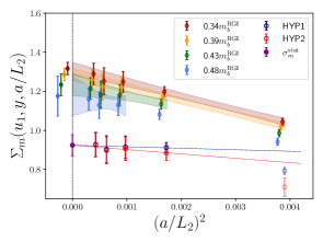
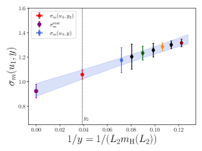
Figure 2: Left: continuum limit extrapolation for the relativistic (diamonds) and static (circles) SSF connecting the volume $L_{1}\to L_{2}=2L_{1}$. In the relativistic regime we show only a subset of the available heavy masses to improve readability. In the static theory we make use of two different actions $\mathrm{HYP}1$ and $\mathrm{HYP}2$ to constrain the continuum limit. Right: interpolation between static and relativistic continuum SSF to the physical point $y_{2}$. The colour code is the same in both plots.

2.3 Relativistic QCD in $L_{1}$

Finally, we compute the function $\Pi_{m}(u_{1},y_{1},a/L)$, the finite $a$ approximant to $\pi$, Eq. (5), in the volume $L_{1}\approx 0.5\ \mathrm{fm}$. Here we simulate very fine lattice spacings $0.008\ \mathrm{fm}\leq a\leq 0.02\ \mathrm{fm}$, directly around $y_{B}$. Again we assume a linear dependence on $a^{2}$ to parametrise the cutoff effects at quark masses between $0.9m_{b}$ and $1.1m_{b}$. The continuum extrapolation together with the following linear interpolation in $y$ to the physical point $y_{1}$ are shown in Fig. 3. We observe a remarkably weak dependence on the lattice spacing. To a significant part this is due to the use of a massive scheme for $Z$ and $b_{\mathrm{m}}$ [20].

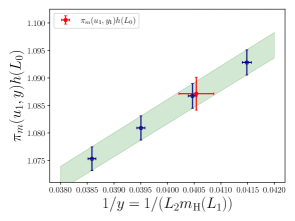
Figure 3: Left: continuum extrapolation of $\Pi_{m}(u_{1},y,a/L_{1})$ at four different masses around the b-quark region in the finite volume $L_{1}$. A fifth available coarsest lattice spacing is excluded from the fit. Right: interpolation to the target b-quark scale $y_{1}$.

We can now evaluate Eq. (2) to quote our preliminary result

$$m_{b}^{\mathrm{RGI}}(N_{f}=3)=6.608(49)\ \mathrm{GeV}\ [0.7\%]\,,$$ (13)

where we remind the reader that the input is the SU(3) symmetric point in the sea sector. Given experience with very small deviations to that point (see Fig. 4 in [21] and Fig. 8 in [22]), we quote no extra uncertainty but are planning to extend the computation to the physical point in $m_{\pi}$ and $m_{K}$ in the future.

We also quote the b-quark mass in the $\overline{\mathrm{MS}}$ scheme in the $N_{f}=4$ theory,

$$\overline{m}_{b}^{(4)}(\overline{m}_{b})=4.174(30)(12)_{\Lambda}\ \mathrm{GeV},$$ (14)

where the second error arises from $\Lambda^{(3)}_{\overline{\mathrm{MS}}}=341(12)\ \mathrm{MeV}$ [23]. We refer to Fig. 4 for a comparison of our result with other studies and for a summary of the error budget of the computation.

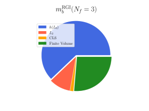
Figure 4: Left: comparison of our results for $\overline{m}_{b}(\overline{m}_{b})$ with FLAG averages and results from other collaborations. For $N_{f}=2+1+1$ [24] the determinations [25, 26, 27, 28, 29, 30, 31] contribute to the average. For $N_{f}=2+1$ [24] results, converted to $N_{f}=4$, are taken from: HPQCD10 [32], HPQCD 13B [33], Maezawa 16 [34], Petreczky [35]. Only the green filled points contribute to the FLAG average. For $N_{f}=2$ [36] the values contributing to the average are: [37, 38, 39]; they are of course not converted to the $N_{f}=4$ theory. The PDG value [11] is converted from their $N_{f}=5$ result to $N_{f}=4$. Right: contribution to the variance of $m_{b}^{\mathrm{RGI}}$. The dominant error source comes from the non-perturbative running factor $h(L_{0})$ [14], followed by the finite volume measurements and the reference scale $L_{\mathrm{ref}}=L_{2}\approx 1.0\ \mathrm{fm}$. Other contributions arising from CLS ensembles are by far subleading at present.

3 $B^{(\star)}$ leptonic decays

As discussed in [1], our strategy is also suited for the extraction of decay constants, using the already determined quark mass proxies $y_{i}$. Here we present results for the vector meson decay constant $f_{B^{\star}}$, which in our strategy plays a crucial role in a precise determination of $b\to u$ semi-leptonic decays, and the pseudo-scalar $f_{B}$, used as a relevant crosscheck of our strategy. Given the axial-vector and vector heavy-light currents $A_{\mu},V_{\mu}$, we define the dimensionless observable used to build the SSF as

$$\Phi_{A_{0}(\vec{V})}(u,y)=\ln\bigg{(}\frac{L_{\mathrm{ref}}^{3/2}}{\sqrt{2}}\hat{f}_{B^{(\star)}}\bigg{)},\qquad\hat{f}_{B^{(\star)}}=\sqrt{m_{B^{(\star)}}}f_{B^{(\star)}},$$ (15)

where in the finite volume the matrix elements are constructed from correlation functions with Schrödinger functional boundary conditions [40, 41, 1]. The step scaling chain takes the form

$$\ln\bigg{(}\frac{L_{\mathrm{ref}}^{3/2}}{\sqrt{2}}\hat{f}_{B^{(\star)}}\bigg{)}=\Phi_{A_{0}(\vec{V})}(u_{1},y_{1})+\sigma_{A_{0}(\vec{V})}(u_{1},y_{2})+\rho_{A_{0}(\vec{V})}(u_{2},y_{B}),$$ (16)

in terms of the SSFs

$$\sigma_{A_{0}(\vec{V})}(u_{1},y) = \Phi_{A_{0}(\vec{V})}(u_{2},y)-\Phi_{A_{0}(\vec{V})}(u_{1},y),$$ (17)

$$\rho_{A_{0}(\vec{V})}(u_{2},y) = \Phi_{A_{0}(\vec{V})}(y)-\Phi_{A_{0}(\vec{V})}(u_{2},y).$$ (18)

Their lattice approximants $\Sigma,R$ use the same LCPs as before and we take their continuum limits in the exact same way. In Fig. 5 the interpolations for $\sigma_{A_{0}(\vec{V})}$ and $\rho_{A_{0}(\vec{V})}$ to the known $y_{2}$ and $y_{B}$ are shown, again with a second order polynomial in $1/y$. It is worth noting that in the $m_{h}\to\infty$ limit spin symmetry means that vector and pseudo-scalar share the same step scaling functions: $\sigma^{\mathrm{stat}}_{A_{0}}=\sigma^{\mathrm{stat}}_{\vec{V}}$ and $\rho^{\mathrm{stat}}_{A_{0}}=\rho^{\mathrm{stat}}_{\vec{V}}$.

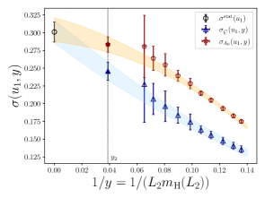
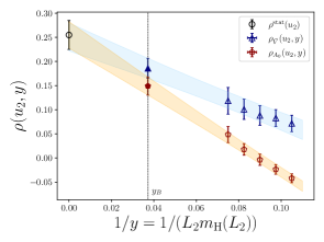
Figure 5: Interpolation to the target b-quark scale for the step $L_{1}\to L_{2}$ (left) and $L_{2}\to\mathrm{CLS}$ (right). Blue triangles and red pentagons correspond to the vector and pseudo-scalar meson decays relativistic SSF, respectively, while the black circles are the shared static $\sigma^{\mathrm{stat}}$ and $\rho^{\mathrm{stat}}$.

For the flavour averaged combinations we arrive at preliminary results

$$f_{\overline{B}}=205.4(4.7)\ \mathrm{MeV}\ [2.2\%],\qquad f_{\overline{B}^{\star}}=207.0(5.4)\ \mathrm{MeV}\ [2.6\%].$$ (19)

We observe that all the steps involved in the computation contribute significantly to the $f_{\overline{B}^{(\star)}}$ error budget, and increased precision can be reached with additional statistics. In contrast to the quark mass, now also our 200% error for $c_{A}^{\mathrm{stat}}$ plays a significant role.

An additional interesting quantity that we can extract with our strategy is the ratio $f_{{\overline{B}}^{\star}}/f_{\overline{B}}$. The latter is obtained from the step scaling chain

$$\ln\bigg{(}\frac{\hat{f}_{\overline{B}}}{\hat{f}_{{\overline{B}}^{\star}}}\bigg{)}=\Phi_{A_{0}/\vec{V}}(u_{1},y_{1})+\sigma_{A_{0}/\vec{V}}(u_{1},y_{2})+\rho_{A_{0}/\vec{V}}(u_{2},y_{B}),$$ (20)

where we use the ratio between pseudo-scalar and vector matrix elements and $\sigma_{A_{0}/\vec{V}}=\sigma_{A_{0}}-\sigma_{\vec{V}}$, etc. We report the interpolation results to the target $y_{i}$ in Fig. 6. Here we have $\rho_{A_{0}/\vec{V}}^{\mathrm{stat}}=\sigma_{A_{0}/\vec{V}}^{\mathrm{stat}}=0$, imposing a strong constraint on the interpolation formula. Our preliminary result,

$$f_{\overline{B}^{\star}}/f_{\overline{B}}=0.999(19)\ [1.9\%]\,,$$ (21)

happens to be in agreement with the static value of one, but it is derived from individual pieces with few percent $1/m$ corrections which cancel only in the final quantity. A comparison with other determinations is shown in Fig. 7.

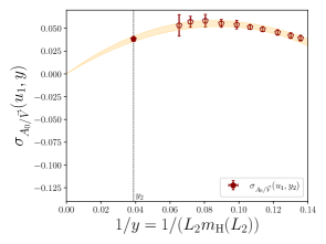
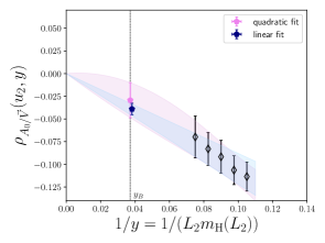
Figure 6: Interpolation of the ratio $f_{\overline{B}}/f_{{\overline{B}}^{\star}}$ to the target b-quark scale for the steps $L_{1}\to L_{2}$ (left) and $L_{2}\to\mathrm{CLS}$ (right). On the right plot we show results from both a linear and quadratic fit. We use the latter in our determination as conservative choice.

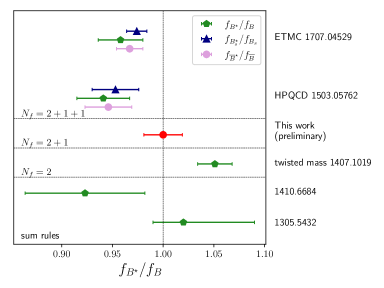
Figure 7: Results comparison for the ratio between vector and pseudo-scalar meson decays. Blue triangles correspond to $f_{B_{s}^{\star}}/f_{B_{s}}$, green pentagons to $f_{B^{\star}}/f_{B}$, while pink circles show the flavour averaged combination of the ratio $f_{{\overline{B}}^{\star}}/f_{\overline{B}}$. Starting from the bottom, results are taken from: [42, 43, 44, 45, 46].

4 Conclusion and Outlook

We have demonstrated the applicability of the strategy presented in [1] by combining static and relativistic computations in the continuum to reach the physical b-quark mass by interpolation. We presented preliminary results for the RGI b-quark mass, pseudo-scalar and vector meson decay constants, demonstrating the potential of this approach to achieve high-precision results with minimal assumptions.

Looking ahead, the future trajectory of this research involves extending computations to lighter pion mass ensembles, to reach the physical point also in this variable. Furthermore, ongoing efforts are directed towards determining the $c_{A}^{\mathrm{stat}}$ improvement coefficient for the Lüscher-Weisz gauge action. Studies of systematic effects related to the variations of the functional forms used for the continuum-limit extrapolation [47, 48, 49] and for the interpolation to the target b-quark scale, as well as different definitions of the finite volume observables, will be considered.

We note that the result for the vector meson decay constant can be employed for a precise determination of the $b\to u$ semi-leptonic form factor $f_{\perp}$ as pointed out in [1]. All finite volume step scaling quantities are extrapolated to the continuum limit and do not need to be repeated with discretisations used for the form factor computations. An accurate knowledge of these quantities is required to deepen our knowledge of the SM and to test for new physics phenomena.

References

- [1] R. Sommer et al., PoS LATTICE2023 (2023) 268.
- [2] D. Guazzini, R. Sommer and N. Tantalo, JHEP 01 (2008) 076 [0710.2229].
- [3] M. Bruno et al., JHEP 02 (2015) 043 [1411.3982].
- [4] M. Bruno, T. Korzec and S. Schaefer, Phys. Rev. D 95 (2017) 074504 [1608.08900].
- [5] D. Mohler, S. Schaefer and J. Simeth, EPJ Web Conf. 175 (2018) 02010 [1712.04884].
- [6] D. Mohler and S. Schaefer, Phys. Rev. D 102 (2020) 074506 [2003.13359].
- [7] J. Heitger and R. Sommer, Nucl. Phys. B Proc. Suppl. 106 (2002) 358 [hep-lat/0110016].
- [8] G. M. de Divitiis, M. Guagnelli, R. Petronzio et al., Nucl. Phys. B 675 (2003) 309 [hep-lat/0305018].
- [9] M. Dalla Brida, P. Fritzsch, T. Korzec et al., Phys. Rev. D 95 (2017) 014507 [1607.06423].
- [10] P. Fritzsch, J. Heitger and S. Kuberski, PoS LATTICE2018 (2018) 218 [1811.02591].
- [11] P. A. Zyla et al., PTEP 2020 (2020) 083C01.
- [12] M. Bruno, M. Dalla Brida, P. Fritzsch et al., Phys. Rev. Lett. 119 (2017) 102001 [1706.03821].
- [13] S. Kuberski, , Standard Model parameters in the heavy quark sector from three-flavor lattice QCD, Ph.D. thesis, "U. Münster", 2020.
- [14] I. Campos, P. Fritzsch, C. Pena et al., Eur. Phys. J. C 78 (2018) 387 [1802.05243].
- [15] M. Lüscher, S. Sint, R. Sommer et al., Nucl. Phys. B 478 (1996) 365 [hep-lat/9605038].
- [16] T. Bhattacharya, R. Gupta, W. Lee et al., Phys. Rev. D 73 (2006) 034504 [hep-lat/0511014].
- [17] A. Grimbach, D. Guazzini, F. Knechtli et al., JHEP 03 (2008) 039 [0802.0862].
- [18] A. Hasenfratz and F. Knechtli, Phys. Rev. D 64 (2001) 034504 [hep-lat/0103029].
- [19] M. Della Morte, S. Dooling, J. Heitger et al., JHEP 05 (2014) 060 [1312.1566].
- [20] P. Fritzsch, J. Heitger and S. Kuberski, , Heavy valence Wilson fermions with effective mass-improvement, to be published, 2024.
- [21] J. Heitger, F. Joswig and S. Kuberski, JHEP 05 (2021) 288 [2101.02694].
- [22] A. Bussone, A. Conigli, J. Frison et al., 2309.14154.
- [23] M. Bruno, M. D. Brida, P. Fritzsch et al., Phys. Rev. Lett. 119 (2017) 102001.
- [24] Y. Aoki et al., Eur. Phys. J. C 82 (2022) 869 [2111.09849].
- [25] D. Hatton, C. T. H. Davies, J. Koponen et al., Phys. Rev. D 103 (2021) 114508 [2102.09609].
- [26] A. Bazavov et al., Phys. Rev. D 98 (2018) 054517 [1802.04248].
- [27] P. Gambino, A. Melis and S. Simula, Phys. Rev. D 96 (2017) 014511 [1704.06105].
- [28] A. Bussone et al., Phys. Rev. D 93 (2016) 114505 [1603.04306].
- [29] B. Colquhoun, R. J. Dowdall, C. T. H. Davies et al., Phys. Rev. D 91 (2015) 074514 [1408.5768].
- [30] A. Bussone et al., Nucl. Part. Phys. Proc. 273-275 (2016) 1638 [1411.0484].
- [31] B. Chakraborty, C. T. H. Davies, B. Galloway et al., Phys. Rev. D 91 (2015) 054508 [1408.4169].
- [32] C. McNeile, C. T. H. Davies, E. Follana et al., Phys. Rev. D 82 (2010) 034512.
- [33] A. J. Lee, C. J. Monahan, R. R. Horgan et al., Phys. Rev. D 87 (2013) 074018.
- [34] Y. Maezawa and P. Petreczky, Phys. Rev. D 94 (2016) 034507.
- [35] P. Petreczky and J. H. Weber, Phys. Rev. D 100 (2019) 034519.
- [36] S. Aoki et al., Eur. Phys. J. C 77 (2017) 112 [1607.00299].
- [37] N. Carrasco et al., JHEP 03 (2014) 016 [1308.1851].
- [38] F. Bernardoni et al., Phys. Lett. B 730 (2014) 171 [1311.5498].
- [39] P. Dimopoulos et al., JHEP 01 (2012) 046 [1107.1441].
- [40] M. Lüscher, R. Narayanan, P. Weisz et al., Nucl. Phys. B 384 (1992) 168 [hep-lat/9207009].
- [41] S. Sint, Nucl. Phys. B 421 (1994) 135 [hep-lat/9312079].
- [42] P. Gelhausen, A. Khodjamirian, A. A. Pivovarov et al., Phys. Rev. D 88 (2013) 014015 [1305.5432].
- [43] W. Lucha, D. Melikhov and S. Simula, EPJ Web Conf. 80 (2014) 00046 [1410.6684].
- [44] D. Becirevic, A. Le Yaouanc, A. Oyanguren et al., 1407.1019.
- [45] B. Colquhoun, C. T. H. Davies, R. J. Dowdall et al., Phys. Rev. D 91 (2015) 114509 [1503.05762].
- [46] V. Lubicz, A. Melis and S. Simula, Phys. Rev. D 96 (2017) 034524 [1707.04529].
- [47] N. Husung, P. Marquard and R. Sommer, Eur. Phys. J. C 80 (2020) 200 [1912.08498].
- [48] N. Husung, P. Marquard and R. Sommer, Phys. Lett. B 829 (2022) 137069 [2111.02347].
- [49] N. Husung, Eur. Phys. J. C 83 (2023) 142 [2206.03536].