Liquid Surfaces with Chaotic Capillary Waves Exhibit an Effective Surface Tension

Abstract

The influence of chaotic capillary waves on the time-averaged shape of a liquid volume is studied experimentally and theoretically. In that context, a liquid film containing a stable hole is subjected to Faraday waves. The waves induce a shrinkage of the hole compared to the static film, which can be described using the Young-Laplace equation by incorporating an effective capillary length. In the regime of chaotic Faraday waves, the presented theory explains the hole shrinkage quantitatively, linking the effective capillary length to the wave energy. The effect of chaotic Faraday waves can be interpreted as a dynamic surface force that acts against surface tension.

Out-of-equilibrium liquid surfaces exhibit very rich and intriguing dynamics. A common way to excite dynamic modes on a liquid surface is to vibrate a liquid volume. The mean (time-averaged) free surface of a vibrated liquid volume can take shapes that are significantly different from that in equilibrium [1, 2]. Further, by vibrating a liquid, its stability behavior can be influenced and unstable modes can be eliminated in specific parameter regimes. For example, the Rayleigh-Taylor instability of superposed liquids can be suppressed by vibrating the system normal to the interface [3], or a liquid bridge arranged vertically between two disks can be stabilized by vibrating the upper disk [4]. Vibrating an entire liquid volume is not the only way to excite dynamic modes on a liquid surface. Surprisingly, when exposing a sessile drop to ultrasound, capillary waves are observed on the surface of the drop that have a much lower frequency than the excitation source [5, 6]. A few attempts have been made to explain the nonlinearities that cause the corresponding energy transfer from high to low frequency modes [7, 8].

A classical configuration used to create capillary waves on a liquid is to vibrate a liquid pool at a comparatively low frequency of a few 100 Hz or smaller. Above a critical acceleration amplitude, so-called Faraday waves are observed  [9, 10], a phenomenon that has been studied intensely during the past decades. The classical configuration, however, gives little information about how such surface waves can affect the time-averaged shape of a liquid volume. Corresponding information can be obtained when a drop is deposited on a liquid pool that is vibrated, such that Faraday waves can be excited on the drop surface, while the surface of the pool remains below the excitation threshold [11, 12]. Two regimes are observed: A quasi-steady regime in which the drop takes a new (time-averaged) equilibrium shape and a second unsteady regime in which the drop shape exhibits large variations in time. One fundamental challenge related to capillary waves is the question whether the complex dynamics of such systems can be captured by simplified theoretical descriptions. In the simplest case, important aspects of the dynamics would be captured by mapping the system to a stationary equilibrium system with effective parameters. An important step in that direction was made by Welch et al. who studied chaotic Faraday waves on a liquid pool [13, 14]. They showed that a probe immersed in the liquid behaves as if the liquid has an effective temperature and viscosity. These quantities are tunable via the frequency and amplitude of the shaker.

In the present work, we consider a similar situation as in [13], but focus on surface properties of the liquid instead of bulk properties. Specifically, we will show that a liquid volume on which chaotic Faraday waves are excited behaves as if it possesses an effective surface tension that can be tuned via the frequency and amplitude of the shaker. In that context, the dynamic system can be mapped to a static equilibrium system that is described by the Young-Laplace equation. Consider a bounded film of water on a horizontal surface. In this configuration we can create a defect or hole in the liquid film that is stable [15]. Above a critical radius we can vary the size of the hole by changing the liquid volume inside the container [16]. Using a superhydrophobic substrate [17] we obtain a rather thick film ($h\approx\qty{5}{\milli}$) that is very sensitive to disturbances by external forces. This makes it an ideal candidate to study the effect of capillary waves on the time-averaged shape of the free-surface. When subjecting this system to vertical vibrations, as shown in Fig. 1, we see concentric patterns of boundary waves for low excitation amplitudes. When surpassing a critical amplitude we see Faraday waves that become more chaotic with increasing amplitude. The time-averaged diameter of the hole shrinks continuously with increasing amplitude.

Figure 1: Stable holes in vibrated liquid films shrinking with increasing excitation amplitude. The plot on the left shows the normalized time-averaged hole diameter as a function of the dimensionless acceleration amplitude and corresponds to the images on the right. The error bars show the standard deviation for subsequent measurements. $f_{\mathrm{ex}}=\qty{170}{}$, $d_{\mathrm{static}}$=24.6 and $a_{\mathrm{max}}=\qty{68.36}{\per\square}$.

In a second set of experiments we keep the vibration amplitude constant and instead slowly add liquid to the film. The resulting hole diameter is shown in Fig. 2. Remarkably, the dynamic system evolves very similarly as the static one. The hole shrinks with increasing volume. Using the Young-Laplace equation we can describe how the hole in the static film should evolve in this $d$-$V$-space. Comparing the Young-Laplace model with the experimental results it seems as if the dynamic system behaves as if it has an effective capillary length. In combination with the results shown in Fig. 1 it is natural to assume that the effective capillary length also depends systematically on the wave dynamics. This raises two important questions: How exactly is this effective capillary length related to the wave dynamics, and is there a physically meaningful interpretation of it?

Figure 2: Evolution of the hole diameter with liquid volume in the film. The black and magenta curves show experimental data obtained from a static film and a vibrated one, respectively. Thin gray lines represent numerical solutions of the Young-Laplace equation for different capillary lengths. $f_{\mathrm{ex}}=\qty{116}{}$, $A_{\mathrm{ex}}\omega_{\mathrm{ex}}=\qty{0.056}{\per}$

To answer these questions, we start with the well established model for the static axisymmetric configuration, similar as in [16]. The pressure jump across the gas-liquid interface is described by the Young-Laplace equation and balances the hydrostatic pressure inside the liquid film

$$-\sigma\left(\diff{\phi}{s}+\frac{\sin{\phi}}{r} =-\rho gz+\Delta p_{0},$$ (1)

where surface tension, mass density and gravity are denoted by $\sigma$, $\rho$ and $g$, respectively. The radial and vertical coordinates are $r$ and $z$, where $z(r)$ describes the liquid surface. The arc-length coordinate along the liquid surface is denoted by $s$, the local inclination angle of the surface by $\phi$. Additionally, we have $\mathrm{d}r/\mathrm{d}s=\cos{\phi}$ and $\mathrm{d}z/\mathrm{d}s=\sin{\phi}$. The Laplace pressure at the solid surface ($z=0$) is denoted by $\Delta p_{0}$. The boundary conditions are $\phi|_{s=0}=\theta$, $r|_{s=0}=r_{0}$, $z|_{s=0}=0$ and $z|_{r=R}=z_{R}$, where $\theta$, $r_{0}$, and $R$ are the contact angle, hole radius and container radius, respectively. The latter boundary condition corresponds to pinning the liquid film to a sharp edge at the perimeter (c.f. Fig. 1). The problem can be non-dimensionalized to depend only on the contact angle and the capillary length $l_{c}=\sqrt{\sigma/\rho g}$.

To describe the dynamics of the film with capillary waves, we introduce an effective capillary length $l_{c}^{\mathrm{eff}}$ and aim at modeling its time-averaged configuration using a static surrogate system described by equation 1. For simplicity, we neglect the second curvature term $\sin(\phi)/r$ in equation 1, which is justified for holes that are large compared to the film height. As a consequence, we can resort to a 2D liquid puddle, as shown in Fig. 3. The liquid puddle height $h$ depends on the hydrostatic pressure inside the film, surface tension and the contact angle. Balancing the forces in horizontal direction gives

$$h=\sqrt{2(1-\cos{\theta})\cdot l_{c}^{\>2}}$$ (2)

for the static liquid puddle [18]. In order to apply this model to the dynamic system with capillary waves, we need to compute the effective capillary length. We introduce a horizontal force $S_{\mathrm{rad}}$ (c.f. Fig. 3 A) that acts in addition to surface tension, far away from the meniscus, and represents the dynamic contribution of the waves. Considering the horizontal force balance at the liquid surface, we obtain a modified expression for the capillary length:

$$l_{c}^{\mathrm{eff}}=\sqrt{l_{c}^{2}-\frac{S_{\mathrm{rad}}}{\rho g(1-\cos{\theta})}}.$$ (3)

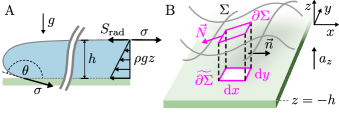
Figure 3: Liquid puddle model introducing the effective capillary length (A), and control volume in the deformed liquid film considered to compute $S_{\mathrm{rad}}$ (B). Only forces that act in the horizontal direction are shown.

Next, we study how $S_{\mathrm{rad}}$ depends on the waves in the liquid film. Analyses on the excess momentum flux in capillay wave systems have been performed before, e.g. by Longuet-Higgins and Stewart [19]. In analogy to the pressure that electromagnetic waves exert onto surfaces, this additional momentum flux is often called radiation pressure or radiation stress in the anisotropic case. This radiation pressure can be related to the area specific energy contained in the waves. This is explained in detail in the Supplementary Material [20]. The most important steps in the calculation of $S_{\mathrm{rad}}$ are outlined in the following.

We consider the system shown in Fig. 3 B that is based on an infinitely extended film. We parameterize the surface $\Sigma$ by a height function $z=\eta(x,y,t)$ that describes the displacement relative to the static film for which we have $z=0$. The liquid film is subject to a time-harmonic vertical acceleration

$$a_{z}=-g+A_{\mathrm{ex}}\omega_{\mathrm{ex}}^{2}\cos{\left(\omega_{\mathrm{ex}}t\right)}.$$ (4)

We assume that the induced waves are chaotic such that

$$\left\langle\eta(x,y,t)\right\rangle_{t}=0,$$ (5)

where $\langle\cdot\rangle_{t}$ denotes local time averaging over a period much larger than a wave period. Further, we assume that for the dynamic system $\partial/\partial{}t\left\langle\cdot\right\rangle_{t}=0$ holds for all field quantities. Therefore, for the dynamic system the time-averaged momentum flux into the volume shown in Fig. 3 B is zero. Assuming the flow to be inviscid, the $x$-momentum balance over the control volume reads

$$0=\left\langle\>\int\displaylimits_{\partial V}\left(\rho uvn_{y}+\rho u^{2}n_{x}+pn_{x}\right)\mathop{}\!\mathrm{d}A-\int\displaylimits_{\partial\Sigma}\sigma N_{x}\mathop{}\!\mathrm{d}s\right\rangle_{t},$$ (6)

where $u,v$ denote the $x,y$-components of the velocity field, respectively, $p$ pressure, $n_{x},n_{y}$ the components of the outward unit normal vector on the control volume, and $N_{x}$ is the $x$-component of the tangent unit vector at the liquid surface normal to $\partial\Sigma$. Assuming the waves and the velocity field to be statistically isotropic in the horizontal plane the shear-stress contribution from the first term in the integral vanishes. It also implies that we do not loose generality by examining only the $x$-direction. Using the small angle approximation for the liquid surface we obtain $N_{x}=\cos\left(\partial\eta/\partial x\right)$ and $\mathrm{d}y=\cos\left(\partial\eta/\partial y\right)\mathrm{d}s$. Splitting the integration over $\partial{}V$ into one over the time-independent line $\widetilde{\partial\Sigma}$ (c.f. Fig. 3B) and the film height, we pull the time averaging in equation 6 under the time-independent line integral, giving

$$0=\int\displaylimits_{\widetilde{\partial\Sigma}}\left\langle\Phi_{\mathrm{dyn}}\right\rangle_{t}n_{x}\mathop{}\!\mathrm{d}{}\tilde{s}$$ (7)

where

$$\left\langle\Phi_{\mathrm{dyn}}\right\rangle_{t}=\left\langle\>\int_{-h}^{\eta}\left(\rho u^{2}+p\right)\mathop{}\!\mathrm{d}z-\sigma\frac{\cos{\left(\frac{\partial\eta}{\partial x}\right)}}{\cos{\left(\frac{\partial\eta}{\partial y}\right)}}\right\rangle_{t}$$ (8)

is the height integrated, time averaged horizontal momentum flux per unit area. We define the radiation pressure $S_{\mathrm{rad}}$ as the difference in horizontal momentum flux between the time-averaged dynamic system and the static system

$$\begin{split}S_{\mathrm{rad}}\coloneqq&\left\langle\Phi_{\mathrm{dyn}}\right\rangle_{t}-\left(\int_{-h}^{0}-\rho gz\mathop{}\!\mathrm{d}z-\sigma\right).\end{split}$$ (9)

Exploiting the separation of timescales between the oscillation period and the chaotic motion of the wave patterns, we can assume standing waves. Then we have $\left\langle\cos(\partial\eta/\partial x)/\cos(\partial\eta/\partial y)\right\rangle_{t}=1$. To further simplify equation 9, we split the pressure integral in two at $z=\eta_{\mathrm{min}}=\min{(\eta(x,y,t))}$. Then equation 9 becomes $S_{\mathrm{rad}}=S_{\mathrm{rad}}^{(1)}+S_{\mathrm{rad}}^{(2)}$ with

$$\begin{split}S_{\mathrm{rad}}^{(1)}\coloneqq&\left\langle\int_{-h}^{\eta}\rho u^{2}\mathop{}\!\mathrm{d}z\right\rangle_{t}+\int_{-h}^{\eta_{\mathrm{min}}}\left(\left\langle p\right\rangle_{t}+\rho gz\right)\mathop{}\!\mathrm{d}z\end{split}$$ (10)

and

$$\begin{split}S_{\mathrm{rad}}^{(2)}\coloneqq&\left\langle\int_{\eta_{\mathrm{min}}}^{\eta}p\mathop{}\!\mathrm{d}z\right\rangle_{t}+\int_{\eta_{\mathrm{min}}}^{0}\rho gz\mathop{}\!\mathrm{d}z.\end{split}$$ (11)

We employ a time-averaged vertical momentum balance to reformulate $\left\langle p\right\rangle_{t}$. Further, we assume that $\eta$ does not have a significant frequency component at $\omega_{\mathrm{ex}}$, that the flow is curl-free and that velocity gradients close to the interface are small, such that the pressure inside the first integral of equation 11 is $p=\rho g(\eta-z)-\sigma\kappa$, where we define the sign of the curvature $\kappa$ so that $\kappa<0$ when the liquid film is locally convex. Equations 10 and 11 can then be rewritten as

$$\begin{split}S_{\mathrm{rad}}^{(1)}=&\left\langle\int_{-h}^{\eta}\rho u^{2}\mathop{}\!\mathrm{d}z\right\rangle_{t}-\int_{-h}^{\eta_{\mathrm{min}}}\rho\left\langle w^{2}\right\rangle_{t}\mathop{}\!\mathrm{d}z\end{split}$$ (12)

and

$$\begin{split}S_{\mathrm{rad}}^{(2)}=&\frac{1}{2}\rho g\left\langle\eta^{2}\right\rangle_{t}-\sigma\left\langle\kappa\eta\right\rangle_{t},\end{split}$$ (13)

respectively. For standing waves, the correlation term in equation 13 containing the curvature and film height can be related to the wave number as $\left\langle\kappa\eta\right\rangle_{t}=k^{2}\left\langle\eta\right\rangle_{t}/2$. We can now see that $S_{\mathrm{rad}}^{(2)}$ is equal to the potential energy of the waves. Assuming equipartition between kinetic and potential energy  [21], we have $S_{\mathrm{rad}}^{(1)}\ll S_{\mathrm{rad}}^{(2)}$. Introducing the Bond number $Bo=\rho g/\sigma k^{2}$ and neglecting $S_{\mathrm{rad}}^{(1)}$, we finally arrive at

$$S_{\mathrm{rad}}=\frac{1}{2}\rho g\left\langle\eta^{2}\right\rangle_{t}\left(1+Bo^{-1}\right)=\frac{E}{2},$$ (14)

where $E$ is the total wave energy per unit area. For $Bo^{-1}\gg 1$, the main contribution to the radiation pressure stems from the term $\sigma\left\langle\kappa\eta\right\rangle_{t}$ in equation 13, i.e. the fact that that pressure fluctuations close to the interface caused by the Laplace pressure are locally correlated with the height of the liquid film. We can trace the origin of the radiation pressure further back to equation 11, showing that for $|\eta_{\mathrm{min}}|/h\ll 1$, this contribution is restricted to regions close to the surface. Correspondigly, we interpret the radiation pressure as a dynamic surface force that acts against surface tension. The model presented above implies the possibility to predict the hole shrinkage in the vibrated liquid film solely based on the wave energy. For the experimental validation we choose a frequency range of $\qty{100}{}\leq f_{\mathrm{ex}}\leq\qty{200}{}$, with velocity amplitudes of $0\leq A_{\mathrm{ex}}\omega_{\mathrm{ex}}<\qty{65}{\milli\per}$. This effectively avoids radial oscillation modes and splashing waves, and covers the interval of the expected applicability of our theory. Using the inviscid dispersion relation $\omega^{2}=\tanh{(kh)}\left(gk+(\sigma k^{3})/\rho\right),$ we obtain $Bo^{-1}>8$ for all subharmonic waves. The damping parameter for subharmonic waves is $\gamma=2\nu k_{0}^{2}/\omega_{0}<0.01$. The normalized supercritical amplitude is $\varepsilon\coloneqq(A_{\mathrm{ex}}\omega_{\mathrm{ex}}^{2}-a_{c})/a_{c}<4$, where $a_{c}$ is the critical amplitude. We determine $S_{\mathrm{rad}}$ in two independent ways: First, we follow our hypothesis that we can infer the radiation pressure based on the hole shrinkage. We image the hole in the liquid film from above and determine the diameter of the hole. We record the hole diameter for different amplitudes, frequencies and liquid volumes. Then we estimate the effective capillary lengths of the vibrated systems using a Bayesian hierarchical model involving the Young-Laplace equation via variational inference. Using equation 3, this gives an estimate for $S_{\mathrm{rad}}$ including credibility intervals. Second, we measure the potential energy of the waves and relate it to $S_{\mathrm{rad}}$ via equation 14. To obtain the potential energy we employ a spectral method, which is necessary since a substantial amount of wave energy is found at frequencies above the subharmonic mode. Using a laser sheet triangulation sensor we record a time series of the film height $\eta(x_{0},y_{0},t)$ and determine its power spectral density $\left\langle\eta_{\omega}^{2}\right\rangle_{t}$. Similarly as in [22, 23, 24], we obtain the wave energy spectrum $E_{\omega}$ by

$$E_{\omega}=\rho g\left\langle\eta_{\omega}^{2}\right\rangle_{t}\left(1+Bo^{-1}\right).$$ (15)

The resulting energy spectrum for one parameter combination is shown in figure 4. Via the dispersion relation, the Bond number is a function of $\omega$. The wave energy is given as

$$E=\frac{1}{2\pi}\int_{0}^{\omega_{\mathrm{cut}}}E_{\omega}\mathop{}\!\mathrm{d}\omega.$$ (16)

Weak capillary wave turbulence theory predicts a scaling of $E_{\omega}\propto f^{-3/2}$ (c.f. Fig. 4) [25]. Therefore, the disregarded energy beyond $\omega_{\mathrm{cut}}=\qty{1440}{}$ introduces a relatively small error. For details on the wave energy measurement, the experimental setup and estimation on $S_{\mathrm{rad}}$ the reader is referred to the Supplementary Material [20] (see also references [17, 21, 26, 27, 28, 23, 25, 19] therein).

Figure 4: Experimental results for the area-specific wave energy. The colormap shows the spatially resolved energy spectrum of the vibrated film with a hole at the center. The vertical axis indicates different measurement positions along the radial direction. At the top, the spatially averaged wave spectrum is shown. The blue line indicates the scaling prediction from capillary wave turbulence theory. The total spatially resolved wave energy $E$ is shown on the right. $f_{\mathrm{ex}}=\qty{170}{}$, $A_{\mathrm{ex}}\omega_{\mathrm{ex}}=\qty{57}{\milli\per}$

Fig. 5 shows how $S_{\mathrm{rad}}$ (obtained from hole shrinkage) correlates with $E$.

Figure 5: Comparison between measurement of $S_{\mathrm{rad}}$ via wave energy and estimation of $S_{\mathrm{rad}}$ according to our hypothesis on hole shrinkage. The symbols represent the experimental data, with the marker size and color indicating the hole diameter and excitation frequency, respectively. The error bars correspond to the $\qty{95}{}$ highest posterior density interval (HDPI), see Supplementary Material for details [20]. The magenta line indicates the theoretical prediction. The area left of the dashed line corresponds to boundary waves for which the theory is not applicable.

The prediction according to equation 14 is indicated by the magenta line. As expected, we do not find agreement for low wave energies, where we only have harmonic boundary waves, so that the theory is not applicable. However, when surpassing energies at which Faraday waves start to emerge, we see an increasing agreement between theory and experiments. At large wave energies of $E>\qty{5}{\milli\per}$ we see excellent quantitative agreement. In accordance with the theory, the experimental data do not show any systematic dependency on the hole size (c.f. marker size in Fig. 5) or frequency (c.f. color grading in Fig. 5). The experimental range extends up to wave energies of $E\approx\qty{15}{\milli\per}$ i.e. a radiation pressure of $S_{\mathrm{rad}}\approx\qty{7.5}{\milli\per}$. This corresponds to an effective reduction of the surface tension of more than $\qty{10}{}$. Using this upper bound for the energy and $Bo^{-1}>8$, we obtain $\sqrt{2\left\langle\eta^{2}\right\rangle_{t}}/h<0.11$. Thus, we interpret $S_{\mathrm{rad}}$ as a dynamic surface force. In conclusion, we presented a theory that connects the dynamics of a vibrated liquid film to its static behavior. The surface waves on the film cause a radiation pressure than can be understood as an effective contribution to surface tension. We conducted experiments that are in quantitative agreement with the theory within its expected range of validity. As surface tension can play a pivotal role in the stability of liquid volumes, our findings could explain the stabilizing or destabilizing effects of capillary waves. More generally, the concept of an effective surface tension of vibrated liquids could open the door to far-reaching analogies, such as Marangoni stresses that arise due to variations of the wave energy.

I Acknowledgements

We wish to acknowledge the help by Matthias Weigold, TU Darmstadt, who provided the Laser triangulation sensor for the wave energy measurement. Funding by the Deutsche Forschungsgemeinschaft (DFG, German Research Foundation), Project IDs 459970814, 459970841 and 455566770 is greatly acknowledged. S.B. likes to thank Salar Jabbary Farrokhi for helpful discussions.

References

- Beyer et al. [2001] K. Beyer, I. Gawriljuk, M. Günther, I. Lukovsky, and A. Timokha, Zeitschrift für angewandte Mathematik und Mechanik ZAMM 81, 261 (2001).
- Gavrilyuk et al. [2004] I. Gavrilyuk, I. Lukovsky, and A. Timokha, Zeitschrift für angewandte Mathematik und Physik ZAMP 55, 1015 (2004).
- Wolf [1970] G. Wolf, Physical Review Letters 24, 444 (1970).
- Haynes et al. [2018] M. Haynes, E. Vega, M. Herrada, E. Benilov, and J. Montanero, Journal of Colloid and Interface Science 513, 409 (2018).
- Qi et al. [2008] A. Qi, L. Y. Yeo, and J. R. Friend, Physics of Fluids 20 (2008).
- Tan et al. [2010] M. K. Tan, J. R. Friend, O. K. Matar, and L. Y. Yeo, Physics of Fluids 22 (2010).
- Blamey et al. [2013] J. Blamey, L. Y. Yeo, and J. R. Friend, Langmuir 29, 3835 (2013).
- Zhang et al. [2023] S. Zhang, J. Orosco, and J. Friend, Langmuir 39, 3699 (2023).
- Faraday [1830] M. Faraday, Proceedings of the Royal Society of London 3, 49 (1830).
- Benjamin and Ursell [1954] T. B. Benjamin and F. J. Ursell, Proceedings of the Royal Society of London. Series A. Mathematical and Physical Sciences 225, 505 (1954).
- Pucci et al. [2011] G. Pucci, E. Fort, M. B. Amar, and Y. Couder, Physical Review Letters 106, 024503 (2011).
- Pucci [2015] G. Pucci, International Journal of Non-Linear Mechanics 75, 107 (2015).
- Welch et al. [2016] K. J. Welch, A. Liebman-Peláez, and E. I. Corwin, Proceedings of the National Academy of Sciences 113, 10807 (2016).
- Welch et al. [2014] K. J. Welch, I. Hastings-Hauss, R. Parthasarathy, and E. I. Corwin, Physical Review E 89, 042143 (2014).
- Sharma and Ruckenstein [1990] A. Sharma and E. Ruckenstein, Journal of Colloid and Interface Science 137, 433 (1990).
- Lv et al. [2018] C. Lv, M. Eigenbrod, and S. Hardt, Journal of Fluid Mechanics 855, 1130 (2018).
- Gupta et al. [2016] R. Gupta, V. Vaikuntanathan, and D. Sivakumar, Colloids and Surfaces A: Physicochemical and Engineering Aspects 500, 45 (2016).
- Gennes et al. [2004] P.-G. Gennes, F. Brochard-Wyart, D. Quéré, et al., Capillarity and Wetting Phenomena: Drops, Bubbles, Pearls, Waves (Springer, 2004).
- Longuet-Higgins and Stewart [1964] M. S. Longuet-Higgins and R. Stewart, in Deep Sea Research and Oceanographic Abstracts, Vol. 11 (Elsevier, 1964) pp. 529–562.
- See Supplemental Material [2023] See Supplemental Material, for details on the experimental setup, the wave energy measurement, the estimation on the radation pressure and the derivation of how it depends on the wave energy, which includes refs. [17, 21, 26, 27, 28, 23, 25, 19], http://www.placeholder.de (2023).
- Galtier [2021] S. Galtier, Geophysical & Astrophysical Fluid Dynamics 115, 234 (2021).
- Berhanu and Falcon [2013] M. Berhanu and E. Falcon, Physical Review E 87, 033003 (2013).
- Deike et al. [2014] L. Deike, M. Berhanu, and E. Falcon, Physical Review E 89, 023003 (2014).
- Berhanu et al. [2018] M. Berhanu, E. Falcon, and L. Deike, Journal of Fluid Mechanics 850, 803 (2018).
- Zakharov and Filonenko [1967] V. Zakharov and N. Filonenko, Journal of Applied Mechanics and Technical Physics 8, 37 (1967).
- Hatatani et al. [2022] M. Hatatani, Y. Okamoto, D. Yamamoto, and A. Shioi, Scientific Reports 12, 14141 (2022).
- Huang et al. [2021] E. Huang, A. Skoufis, T. Denning, J. Qi, R. R. Dagastine, R. F. Tabor, and J. D. Berry, Journal of Open Source Software 6, 2604 (2021).
- Przadka et al. [2012] A. Przadka, B. Cabane, V. Pagneux, A. Maurel, and P. Petitjeans, Experiments in Fluids 52, 519 (2012).