The anomaly of the CMB power with the latest Planck data
Abstract
The lack of power anomaly is an unexpected feature observed at large angular scales in the CMB maps by the COBE, WMAP and Planck satellites. This signature, which consists in a missing of power with respect to that predicted by the CDM model, might hint at a new cosmological phase before the standard inflationary era. The main point of this paper is taking the latest Planck polarisation data into account to investigate how CMB polarisation improves the understanding of this feature. With this aim, we apply to the last Planck data, both PR3 (2018) and PR4 (2020) releases, a new class of estimators able to evaluate this anomaly considering temperature and polarisation data both separately and in a jointly way. This is the first time that the PR4 dataset is used to study this anomaly. In order to critically evaluate this feature, taking into account the residuals of known systematic effects present in the Planck datasets, we analyse the cleaned CMB maps using different combinations of sky masks, harmonic range and binning on the CMB multipoles. Our analysis shows that the estimator based only on temperature data confirms the presence of a lack of power with a lower-tail-probability (LTP), depending on the component separation method, and , for PR3 and PR4 respectively. To our knowledge the for the PR3 dataset is the lowest one present in the literature obtained from Planck 2018 data considering the Planck confidence mask. We find significant differences between these two datasets when polarisation is taken into account. However, we also show that for the PR3 dataset the inclusion of the subdominant polarisation information provides estimates which are less likely accepted in a CDM cosmological model than the only-temperature analysis on the whole harmonic-range considered.
1 Introduction
The CMB anomalies are unexpected features observed at large angular scale in the CMB maps (above a few degrees), as observed by the COBE, WMAP and Planck satellites, that deviate from the CDM cosmological model with a statistical significance typically around 2-3 C.L.. These anomalies are not all independent and a certain degree of correlation exists [1]. In particular, the maps of temperature anisotropies exhibit low variance [2], a lack of correlation on the largest angular scales [3], a preference for odd parity modes [4], a hemispherical power asymmetry [5, 6], an alignment between various low multipole moments [7], an alignment between those low multipole moments and the motion and geometry of the Solar System [8], and an unexpected large cold spot in the Southern hemisphere [9]. Historically, the first observed anomalous feature, already within the COBE data, was the smallness of the quadrupole moment. It confirmed to be low when WMAP released its data [10]. However it was also shown that cosmic variance allows for such a small value. Another discovery in the first release of WMAP [10] was that the angular two-point correlation function, at angular scales larger than 60 degrees is unexpectedly close to zero, where a non-zero correlation signal was expected. This feature had already been observed by COBE [11], and was confirmed by WMAP and Planck.
Here we focus on the lack of power anomaly, an intriguing feature that seems to be correlated with a low quadrupole, although it cannot be explained by a lack of quadrupole power alone. This anomaly consists in a missing of power with respect to that predicted by CDM model. An early fast-roll phase of the inflaton could naturally explain such a lack of power, see e.g. [12, 13, 14, 15, 16]: this anomaly might then witness at a new cosmological phase before the standard inflationary era (see e.g. [17, 18, 19]). The explanations for these large-scale CMB features are three: they could have cosmological origins [12], they could be artifacts of astrophysical foregrounds and instrumental systematics or they could be statistical flukes. WMAP and Planck agree well on this feature, so it is very hard, albeit not impossible, to attribute this anomaly to instrumental effects. Moreover it is also difficult to believe that a lack of power could be generated by residuals of astrophysical emission, since the latter is not expected to be correlated with the CMB and therefore an astrophysical residual should increase the total power rather than decreasing it. In addition, in the case of a positive correlation between CMB photons and extra-galactic foregrounds, as seen in [20], a correction for this effect would increase the discrepancy with the model, confirming the CMB lack of power [21]. Hence, it appears natural to accept this as a real feature present in the CMB pattern.
This effect has been studied with the variance estimator in WMAP data [2, 22, 23] and in Planck 2013 [24], Planck 2015 [25] and Planck 2018 [26] data, measuring a lower-tail-probability (LTP) of the order of few per cent. Such a percentage can become even smaller, below , once only regions at high Galactic latitude are taken into account [23]. However, with only the observations based on the temperature map, this anomaly is not statistically significant enough to be used to claim new physics beyond the standard cosmological model. In the previous work [27] the former statement was revisited by also considering polarisation data. The authors proposed a new one-dimensional estimator for the lack of power anomaly capable of taking both temperature and polarisation into account jointly. By applying this estimator on Planck 2015 data (PR2), they found the probability that a random realisation is statistically accepted decreases by a factor two when the polarisation is taken into account. Moreover, they have forecasted that future CMB polarisation data at low- might increase the significance of this anomaly.
The main point here is to deeply investigate how CMB polarisation improves the understanding of this feature, expanding on [27]. With this aim, we apply to the latest Planck data, both PR3 (2018) and PR4 (2020) releases, a new class of estimators, defined starting by the mathematical framework assessed in [27], able to evaluate this anomaly considering temperature and polarisation data both separately and in a jointly way. Up to now lack of power has never been studied with PR4 dataset. As far as we know, [26], [28], and [29] are the only studies which investigate the CMB anomalies with the PR3 dataset, and [6] with the both PR3 and PR4 datasets. As described in [30], compared to the previous releases, the PR3 but in particular the PR4 data really better describe the component in polarisation of CMB: in fact PR3 and PR4 show reduced levels of noise and systematics at all angular scales and an improved consistency across frequencies, particularly in polarisation [30]. In order to critically evaluate this feature, taking into account the residuals of known systematic effects presents in the Planck datasets, we consider the cleaned CMB maps (data and end-to-end simulations) studying different combinations of sky-masks, harmonic range and binning on the CMB multipoles.
The paper is organised as follows: in Section 2 we introduce our new class of estimators for evaluating the lack of power; in Section 3 we describe the datasets and the simulations employed; in Section 4 we present the results on Planck PR3 and PR4 data; conclusions are drawn in Section 5. In addition, in appendix A we give the full derivation of our joint estimator, in appendix B we enter more in details about the transfer function which affects the PR4 polarised signal at the largest angular scales and in appendix C we show the application to latest Planck sevem datasets of the estimator for the lack of power developed in [27].
2 Mathematical Framework
In this section we start briefly recalling the definitions of the normalised angular power spectra (NAPS)[27], then we show how to combine them to derive a new class of estimators for the lack of power, based on the usual definition of the variance of a power spectra in the harmonic space.
2.1 Normalised Angular Power Spectra (NAPS)
In [27], starting from the usual equations employed to simulate temperature and E-mode CMB maps, it has been defined the normalised angular power spectra (henceforth NAPS) and as:
| (2.1) | |||||
| (2.2) | |||||
where is defined as:
| (2.3) |
One can interpret , and as the CMB APS estimated from a CMB experiment under realistic circumstances, i.e. including noise residuals, incomplete sky fraction, finite angular resolution and also residuals of systematic effects. While the spectra , and represent the underlying theoretical model. The expected values for NAPS are:
| (2.4) |
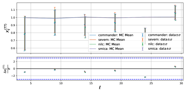
for each . Therefore, the advantage of using NAPS, instead of the standard APS, is that they are dimensionless and similar amplitude numbers. For these reasons they can be easily combined to define 1-D estimators in harmonic space, which depend on temperature, E-mode polarisation and their cross-correlation. In [27], the authors combined the NAPS and to define an optimal, i.e. with minimum variance, estimator called . This estimator, which could be interpreted as a dimensionless normalised mean power, jointly combines the temperature and polarisation data to evaluate the lack of power. In appendix C it is shown its application on the latest Planck dataset.
Finally, here we define two new NAPS:
| (2.5) | |||||
| (2.6) |
with the expected values equal to one. The NAPS and , which depend only on the EE and TE CMB spectra respectively, allow one to define specific estimators able to test the lack of power taking into account only the E-modes and only their cross-correlation with the temperature.
2.2 Variance-based estimators
The idea is to look for estimators sensitive to the variance which are linear in the observed NAPS and also minimum variance.
Starting from the usual definition of the variance of a power spectra, we define the joint estimator , based on the NAPS and :
| (2.7) |
where and are appropriate coefficients associated to each NAPS. Taking the ensemble average of Eq. (2.7) we get:
| (2.8) | |||||
The choice of the value for the constant is totally arbitrary. Thus, its expectation value reads
| (2.9) |
regardless the maximum multipole considered in the analysis.
It is possible to prove that the signal-to-noise ratios of the two NAPS ( and ) are different even in the cosmic variance limit case: therefore one might wonder which are the best coefficients, and , that make the estimator optimal, i.e. with minimum variance. Applying the method of the Lagrange multipliers to minimise the variance of , keeping fixed its expected value (see appendix A for the full derivation), we find that:
| (2.10) | |||||
| (2.11) |
where and are the variances of and respectively, and their covariance:
| (2.12) |
The quantity is defined as:
| (2.13) |
Moreover, in order to evaluate the contribution of each NAPS, we build four analogous optimal estimators which take into account , , and separately:
| (2.14) | |||||
| (2.15) | |||||
| (2.16) | |||||
| (2.17) |
with:
| (2.18) |
where refers to , , or . Their expected values are:
| (2.19) |
regardless the maximum multipole considered in the analysis.
2.3 Implemented formalism
The final expressions of the optimal estimators, given in Eqs. (2.7), (2.14),(2.15), (2.16) and (2.17), are obtained starting from the NAPS at single-, Eqs. (2.1),(2.2),(2.5) and(2.6). However, to reduce any possible correlation effect between different multipoles arising from using a sky mask, we are going to apply a binning on the CMB multipoles.
We estimate the binned expressions of the NAPS by applying the standard operator (see e.g. [31]) 111For a set of bins, indexed by , with respective boundaries , where and mean the lower and the higher multipole in the bin , one can define the binning operator as follows: (2.23) where stands for the minimum multipole considered, which for the CMB it is typically .:
| (2.24) | |||||
| (2.25) | |||||
| (2.26) | |||||
| (2.27) |
Now we use these modified versions of the NAPS to recompute the expressions of the estimators. In particular, the joint estimator becomes:
| (2.28) |
with:
| (2.29) | |||||
| (2.30) | |||||
| (2.31) |
In Eqs. (2.28) and (2.31), for each bin , is defined as:
| (2.32) |
with the number of multipoles included in the bin .
Analogously the binned versions of the estimators , , and are:
| (2.33) | |||||
| (2.34) | |||||
| (2.35) | |||||
| (2.36) |
with:
| (2.37) |
where refers to , , or .
The binned versions of the estimators, as defined in Eqs.(2.28), (2.33), (2.35) and (2.36), will be actually applied to the dataset described in the following section.
For the sake of brevity, in the following, we do not show the results for and for since they provide qualitatively similar results to and respectively, showing that the dominant contribution in the -objects comes from the EE spectra.
3 Planck Datasets
We make use of the CMB-cleaned maps, data and end-to-end simulations, provided by the latest Planck releases, both PR3 (2018) [32] and PR4 (2020) referred also as NPIPE [30]. In order to separate the sky maps into their contributing signals and to clean the CMB maps from foregrounds, the Planck team used for the PR3 dataset, data and simulations, all the four official component separation methods commander, nilc, sevem and smica [33], while for the NPIPE maps it has been applied only the commander and sevem [30] pipelines. To test the robustness of our analysis we perform our estimators, on each Planck 2018 and 2020 pipeline.
The PR3 Monte Carlo (MC) simulations, referred as FFP10, see e.g. [26], are an updated version of the full focal plane simulations described in [34]. The FFP10 dataset contains the most realistic simulations the Planck collaboration provides to characterise its 2018 data. They consist of 999 CMB maps extracted from the current Planck CDM best-fit model, which are beam smoothed and contain residuals of beam leakage [34]. These maps are complemented by 300 instrumental noise simulations for the full mission and for the two data splits: odd-even (OE) rings and the two half-mission (HM) data. These noise simulations, which are provided for each frequency channel, also include residual systematic effects as beam leakage again, ADC non linearities, thermal fluctuations (dubbed 4K fluctuations), band-pass mismatch and others [35]. The FFP10 simulations are processed through the component separation algorithms in the same way as data.
The NPIPE maps represent an evolution of the PR3 dataset: compared to the latter, the PR4 dataset provides a really better description of the CMB polarisation component, showing reduced levels of noise and systematics at all angular scales and improving consistency across frequencies [30]. In addition to the data, it is also provided 400 and 600 MC simulations respectively for commander 222Note that in the case of commander, 400 MC simulation are provided for the Q,U maps. For the temperature only 100 simulated maps are produced and just for the full mission. and for sevem. While the NPIPE commander team provides the signal-plus-noise simulations, the NPIPE sevem team has released separetely the only-signal and only-noise simulated maps for both the detectors-splits, referred as detector A and detector B (or simply A and B). Note that in the NPIPE A and B data splits the systematic effects between the sets are expected to be uncorrelated [30]. However, we remark that PR4 polarisation data at the largest angular scale are affected by a transfer function which reduces the power of the polarised signal (see section 4.3 from [30]). Therefore to ensure fidelity of the science results, we correct for the transfer function the values of the theoretical power spectra TE and EE which enter in the equation of NAPS, (2.2),(2.5) and (2.6), for more details see appendix B and Fig 15.
3.1 Large angular scale maps and power spectra
In our analysis for the PR3 dataset we use the odd-even (OE) splits for both data and FFP10 simulations for all the four Planck component separation methods. Combining the first 300 CMB realisations with the two different OE splits of 300 noise maps we build two MC sets of 300 signal plus noise simulations which do contain also residuals of known systematic effects. For the PR4 dataset we use sevem maps, data and 600 MC simulations, divided in detector A-B splits. In order to use the NPIPE commander products, since the simulated maps for detector-splits are not available for this component separation method in temperature, we build a hybrid set, and we refer to it as hybrid. In particular, we consider the sevem temperature maps and commander polarisation maps, splitted in detector A and detector B, to build the TQU data map with the corresponding 400 MC simulated maps.
PR3 and PR4 maps, available from the Planck Legacy Archive333https://www.esa.int/Planck (PLA), are provided at HEALPix444https://healpix.sourceforge.net [36] resolution , with a Gaussian beam with . Since we are interested in large angular scales, the full resolution maps are downgraded in the harmonic space to lower resolution , according to:
| (3.1) |
where superscripts and stand for input (full resolution) and output (low resolution) maps, respectively; the coefficient is the Gaussian beam and the HEALPix pixel window functions. At the end of the procedure, the harmonic coefficients are used to build maps at resolution with a Gaussian beam with , which corresponds to 2.4 times the pixel size.
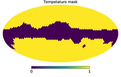
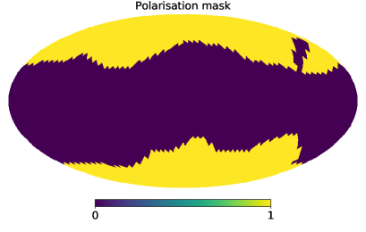
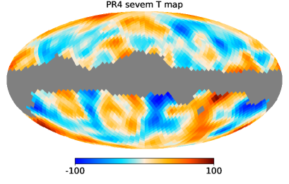
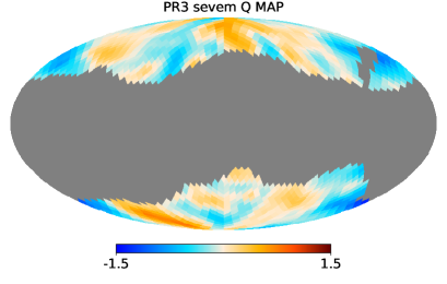
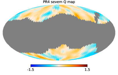
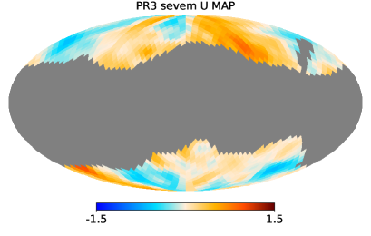
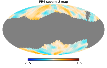
We apply the Planck confidence mask to the temperature maps, while we use a combination of the polarisation confidence mask and the galactic sky mask, provided by Planck, for the polarisation maps. Figure 1 shows the T (left) and P (right) masks at resolution which leave uncovered the and of the sky, respectively. These masks are obtained applying to the full resolution masks 555The masks at resolution are available from the Planck Legacy Archive (PLA). the same downgrading procedure used with the CMB maps and setting a threshold of 0.8 666All the pixels with a value below the threshold are set to 0, while the remaining ones are set to 1. Note that the choice of a larger mask for the polarisation maps is motivated by the fact that using the confidence mask we obtained significant differences in the EE data spectra between different pipelines, most likely due to the impact of the foreground residuals. However, as it is possible to note in the following from Figures 5 and 6, this is not the case if we use the mask in Figure 1. In Figure 2 it is displayed the sevem maps at resolution for both Planck releases.

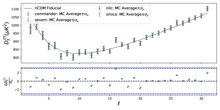
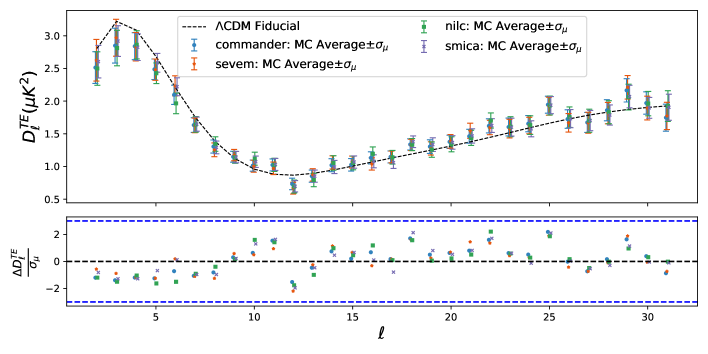
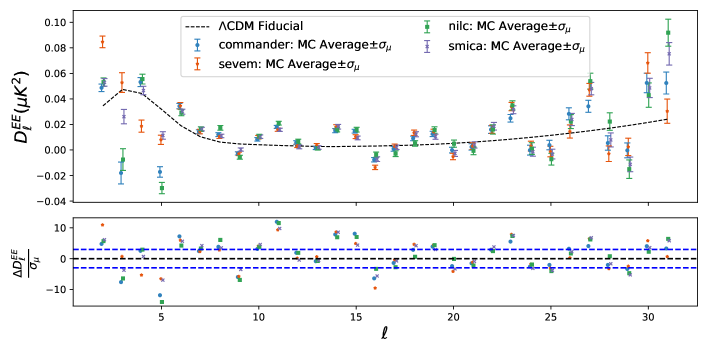
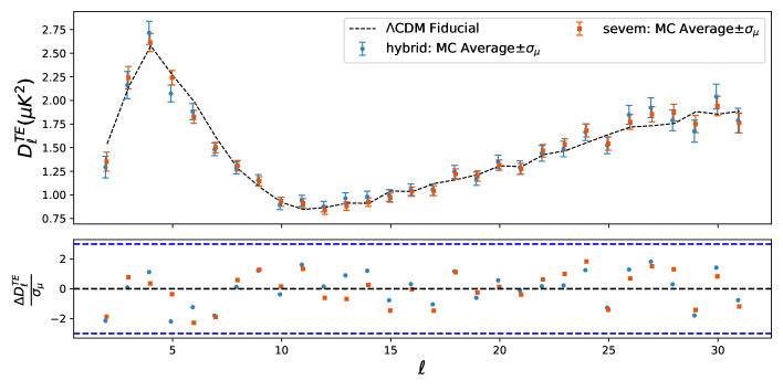
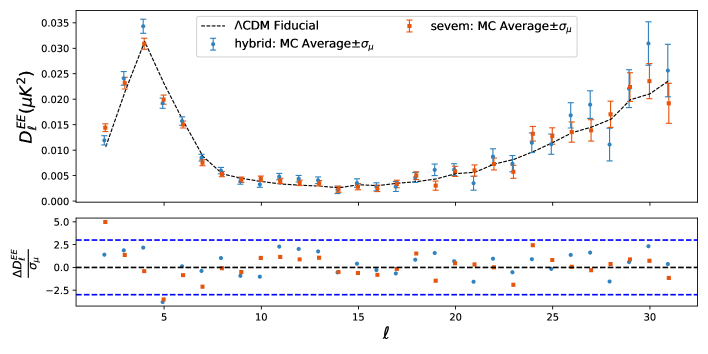
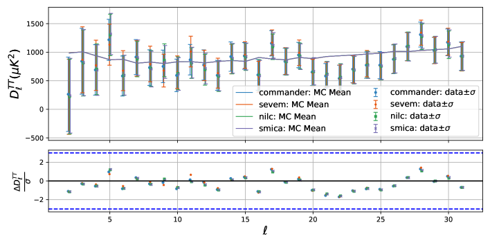
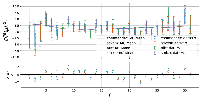
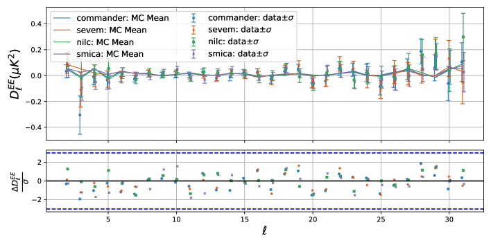
From these maps we estimate the six CMB spectra in cross-mode over the considered sky fraction, in the harmonic range , with the Quadratic-Maximum-Likelihood (QML) estimator ECLIPSE 777https://github.com/CosmoTool/ECLIPSE [37]. Such approach allows us to reduce the residuals of systematic effects and noise bias in the auto-spectra. Figures 3 and 4 characterise the distributions of the TT, TE, EE power spectra obtained from the PR3 and PR4 MC simulations, respectively. In each panel of these figures, the upper box shows the comparison of the MC mean with as error bar of the mean, with respect to the fiducial power spectra. The lower box displays the fluctuations from the theoretical model of the mean in units of . As theoretical model we take into account the Planck 2018 fiducial spectrum [26], defined by the following parameters: , , , , , , , , where . Note that for the PR4 dataset, the TE and EE fiducial spectra have been properly corrected for the NPIPE transfer function (see appendix B). These figures give us information on the systematic effects present in the end-to-end simulations. In particular, for TT and TE spectra the MC mean follows the fiducial for both releases. However, for the case of EE, we find significant deviations for PR3, reflecting the presence of systematics. Conversely, the EE spectrum for PR4 follows, for almost the full range of considered multipoles, the fiducial model, showing the improvement of the PR4 dataset with regard to the level of systematics.

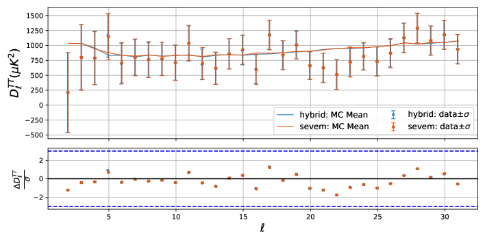
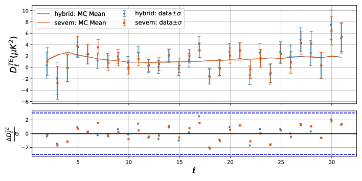
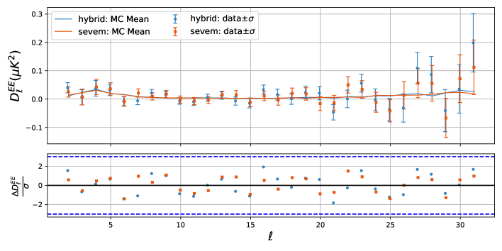
Finally, Figures 5 and 6 show the TT (upper panel), TE (middle panel), EE (lower panel) CMB power spectra obtained from the PR3 and PR4 data as a function of , for . For each plot, in the upper box the points represent the values of the , where , obtained from the data with the standard deviation of the MC distribution as error bar, while the dashed horizontal lines stand for the mean of the MC simulations. Each panel displays also a lower box where for each it is shown the distance of the estimates from the MC mean in units of . From these figures it is possible to note that the data follow in general the mean of the simulations, indicating that the systematics are well characterised in the simulations for both the datasets.
4 Analysis Results
4.1 NAPS with Planck dataset
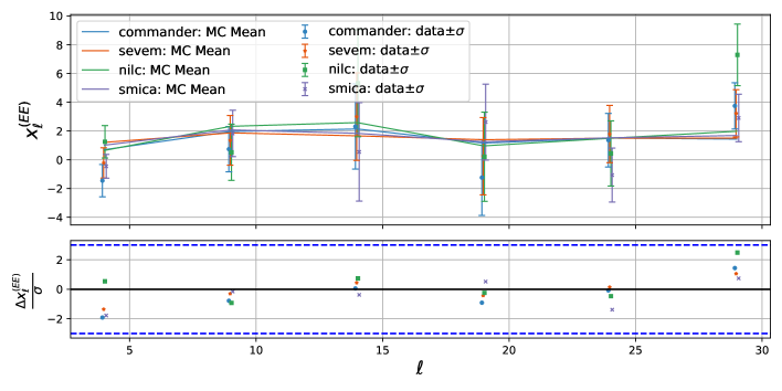
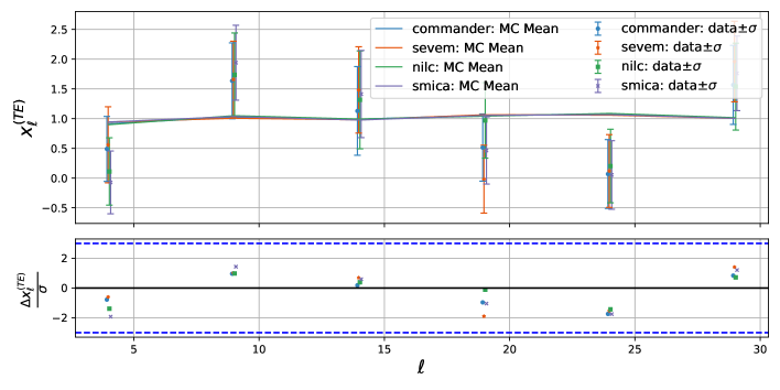
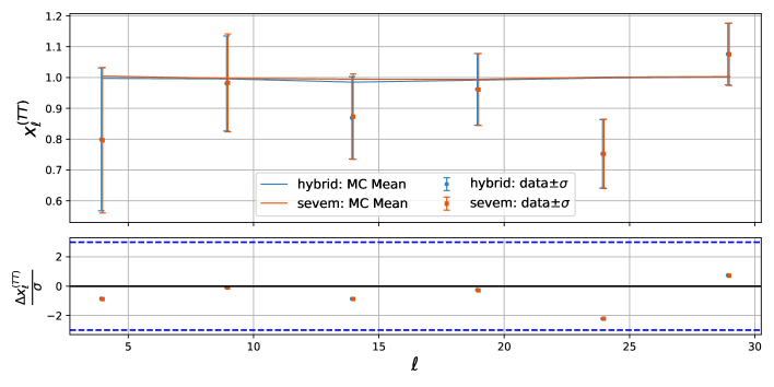
Starting from the angular spectra, computed in the previous section, we build the NAPS, Eqs. (2.24),(2.26) and (2.27), for each MC simulation and for the data, in the harmonic range . In order to reduce any possible correlation effect between different multipoles arising from the mask, we have studied different combinations of binning schemes on the CMB multipoles, choosing a constant bin of . In Figures 7 and 8 the values of the NAPS (upper panel), (middle panel) and (lower panel) are shown for the PR3 and PR4 dataset, respectively. In each panel the upper box displays the values of the data along with the standard deviation of the MC distribution. Each panel displays also a lower box where for each it is shown the distance between the data and the MC mean in units of the uncertainties of the estimates themselves. For both PR3 and PR4, the data follow in general the mean of the simulations, which is around the expected value of 1. However, it is interesting to note the reduction in the estimated error of the binned NAPS for – obtained as the dispersion of the simulations – in PR4. This reflects the improvement in noise and systematics in PR4 with respect to the previous data release.


4.2 Variance-based estimators
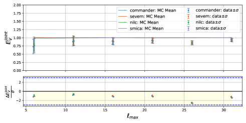
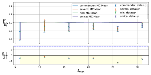
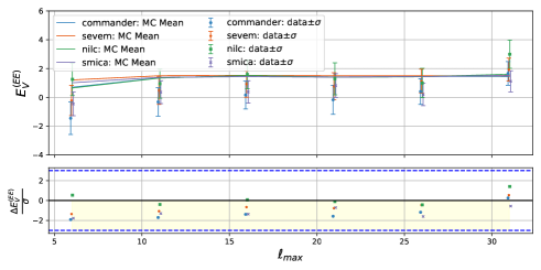
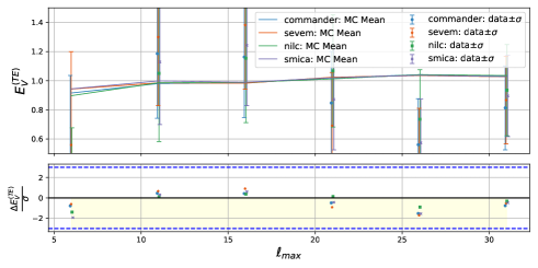
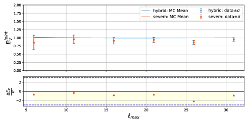
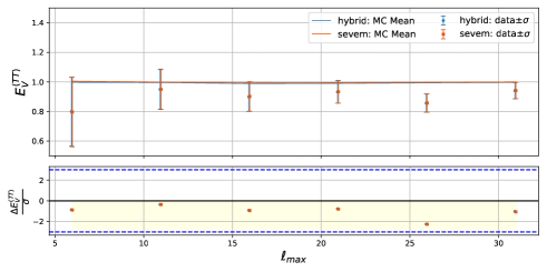
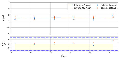
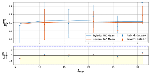
Figures 9 and 10 show (first row), (second row), (third row), (fourth row), defined in Eqs. (2.28), (2.33), (2.35) and (2.36), when applied on the PR3 and PR4 dataset respectively, as a function of the maximum multipole considered in the analysis. In each panel the upper box displays for all the pipelines the values of the data with the standard deviation of the distribution of the simulations as error bars, together with the mean of the MC distribution (solid lines). In the lower panel for each it is shown the difference between the data and the MC mean in units of standard deviation of the MC distribution. If the points are inside the yellow region it means that we are observing less power with respect to that predicted by the model. Note that by applying , , and on PR3 and PR4 dataset, all the values for the first two estimators and the majority for the last two are in the yellow regions. Therefore the Planck data seem to present less power than that expected from the scenario.
In order to quantify the statistical significance of this feature we consider the lower-tail-probability (LTP), defined as:
| (4.1) |
where is the number of simulations with a value equal or smaller than the data value and is the total number of simulations. Thus, Eq.(4.1) provides the probability to obtain a value as low as the data. However, this analysis is limited by the number of MC simulations we have. In particular, we are not able to distinguish between for the PR3 dataset and between and for the hybrid and sevem PR4 pipelines 888We remark that we have 300 simulations for the PR3 pipelines and 400 and 600 simulations for the hybrid and sevem PR4 pipelines, respectively.. If the LTP has a value smaller than the ones aforementioned it just means that the data is lower than all the simulations.
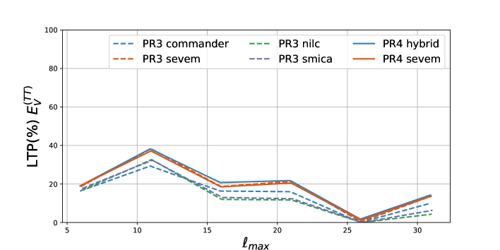
Figure 11 displays the computed for the (upper panel), (middle panel) and (lower panel), applied on the PR3 (dashed lines) and PR4 (solid lines) dataset as a function of .
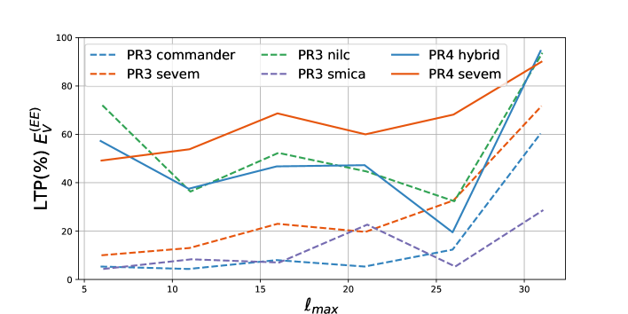
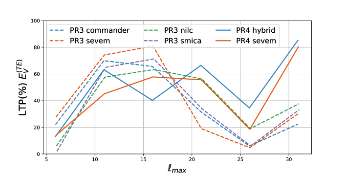
From these plots it is possible to note that:
-
•
with the estimator based only on temperature data, , we find well compatible results between different pipelines and between PR3 and PR4 dataset. The minimum of the LTP is reached at : we confirm the presence of a lack of power with a LTP (PR3) and (PR4), see table 1. To our knowledge, the probability for the PR3 dataset is the lowest one present in the literature obtained from this dataset considering the Planck confidence mask (see Figure 1). Note that, as it has been shown in [22, 23], this anomaly tends to become less significant with increasing sky coverage: in the previous works [25, 26] a LTP below the was measured only when high-latitude galactic regions were taken into account;
-
•
we find significant differences between PR3 and PR4 dataset when polarisation is taken into account through the estimators and . These differences are most likely due to a combination of two factors which are out of our control: a different level of systematics between the PR3 and PR4 dataset and the transfer function which impacts on the PR4 dataset. In fact PR4 data, with respect to PR3 release, better describe the component in polarisation of CMB, providing reduced levels of noise and systematics at all angular scales. However, on the other hand the PR4 polarisation at the largest angular scales are affected by the transfer function which cut the power of the polarised signal, reducing their contribution at those scales;
-
•
note that the estimator based only on EE power spectrum, , at very large scales may exhibit a hint of lack of power when applied to the PR3 data. In particular for the commander and smica pipelines the LTP is for , smaller than the values we get with the estimator based only on temperature data.
Figure 12 displays the computed for the when applied on the PR3 (dashed lines) and PR4 (solid lines) dataset as a function of .
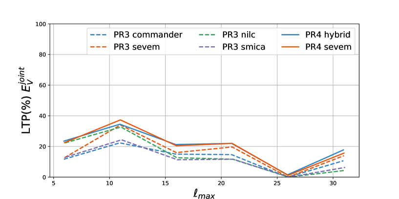
We find well compatible results between different pipelines and between PR3 and PR4 dataset. The trend of the LTP is very similar to the one obtained from , reaching the minimun at (see table 1). Furthermore, for the PR3 dataset, the LTP is smaller than the one measured with at each scale, except for the nilc pipeline. In particular at , applying on the PR3 dataset, we find that no simulation has a value as low as the data for all the pipelines.
| LTP () at | ||||||
|---|---|---|---|---|---|---|
| PR3 | PR4 | |||||
| commander | nilc | sevem | smica | hybrid | sevem | |
In Figure 13 we plot and (see equations (2.29) and (2.30)) as a function of for the PR3 (dashed lines) and PR4 dataset (solid lines) for the sevem pipeline999Similar results are found for all the other pipelines.. Note how for goes to zero because of the noise level in polarisation.
 |
Moreover this plot tells us that in this estimator the largest scales weight much more than small scales, for both the NAPS.
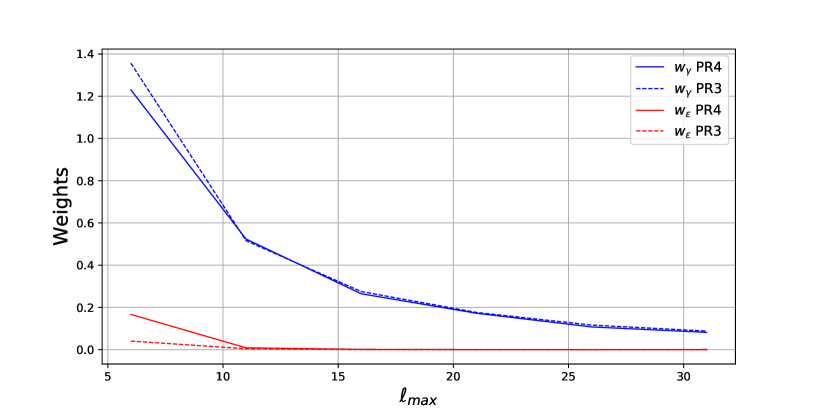
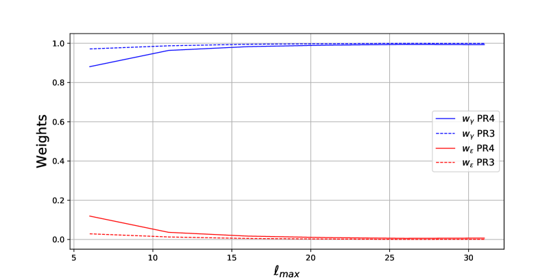
In order to better evaluate the impact of polarisation and temperature data on we define the following weights
| (4.2) | |||||
| (4.3) |
such that for every . For , where the LTP is minimum, we find that polarised PR3 data contribute at the level of to the building of . This value increases to for PR4 polarised data at the same maximum multipole. The behaviour of and for each for the sevem PR3 (dashed lines) and PR4 dataset (solid lines) is given in Figure 14. Even if the contribution of polarisation increases using PR4 data by a factor , the joint analysis is still limited by the noise in Planck polarisation. However, for the PR3 dataset it is interesting to note how the inclusion of the subdominant polarisation part in the analysis makes the LTP of smaller than the one of for the whole harmonic range considered.
5 Conclusions
In this paper we evaluated the lack of power anomaly present at large angular scales of the CMB map considering the latest Planck data, both PR3 (2018) and PR4 (2020) releases. Up to now lack of power has never been studied with PR4 dataset. In particular, our aim was to deeply investigate how CMB polarisation improves the understanding of this anomaly, expanding on the previous work [27].
We have defined and applied on the latest Planck data releases in the harmonic range , a new class of optimised estimators, see Eqs. (2.7), (2.14), (2.15),(2.16) and (2.17), able to test this signature considering temperature and polarisation data both separately and in a jointly way. In order to critically evaluate this feature, taking into account the residuals of known systematic effects present in the Planck datasets, we have considered the cleaned CMB maps (data and end-to-end simulations). Moreover, with the aim of reducing any possible correlation effect between different multipoles arising from the sky mask, we have binned the CMB multipoles with . The main outcomes of this analysis are listed below.
-
1.
The estimator based only on temperature data has confirmed the presence of a lack of power with a LTP (PR3) and (PR4). Note that the for the PR3 dataset is the lowest LTP present in the literature obtained from Planck 2018 data considering the confidence sky mask.
-
2.
We found significant differences between PR3 and PR4 datasets when polarisation is taken into account, most likely due to a combination of two factors: a different level of systematics between the PR3 and PR4 dataset and the transfer function which impacts the PR4 data. However, we have also shown that when the estimator based only on EE power spectrum, , is applied to the PR3 data, and in particular to the commander and smica pipelines, at very large scale we found a LTP for , smaller than the probability we got with the estimator based only on temperature data. Although this behaviour is not statistically significant, it is interesting to note that could point in the direction of a lack of power in large scales also for polarisation. Future observations, such as those from the LiteBIRD satellite, will help to shed light on this result.
-
3.
Considering the joint estimator, , the statement of the LTP is very similar to the one of the probability we got from . At , where the LTP reaches its minimum, we found that the polarised PR3 data contribute at the level of to the total information budget of the estimator. This value increases to for the PR4 polarised data at the same maximum multipole, see Figure 14. Even if the contribution of polarisation increases using PR4 data by factor , the joint analysis is still limited by the noise in Planck polarisation. However, for the PR3 dataset it is interesting to note that the inclusion of polarisation information through the joint estimator has provided estimates which are less likely accepted in a CDM model than the corresponding only-temperature version of the same estimator. In particular, at , we found that no simulation has a value as low as the data for all the pipelines.
Acknowledgements
We thank J.D. Bilbao-Ahedo, C. Gimeno-Amo, A. Gruppuso, R. Keskitalo and P.Vielva, for valuable advice and comments. MB would like to thank the Angela Della Riccia Foundation for the financial support provided under the ADR fellowship 2022 and 2023. We acknowledge partial financial support from the grant PID2019-110610RB-C21 funded by MCIN/AEI/ and from the Red de Investigación RED2022-134715-T funded by MCIN/AEI/10.13039/5011000011033. This research used resources of the National Energy Research Scientific Computing Center (NERSC), a U.S. Department of Energy Office of Science User Facility located at Lawrence Berkeley National Laboratory, operated under Contract No. DEAC02-05CH11231. This work based on observations obtained with Planck (https://www.esa.int/Planck), an ESA science mission with instruments and contributions directly funded by ESA Member States, NASA, and Canada. Some of the results in this paper have been derived using the HEALPix [36] package and ECLIPSE 101010https://github.com/CosmoTool/ECLIPSE code [37].
References
- [1] J. Jones, C.J. Copi, G.D. Starkman and Y. Akrami, The Universe is not statistically isotropic, 2310.12859.
- [2] C. Monteserin, R.B. Barreiro, P. Vielva, E. Martinez-Gonzalez, M.P. Hobson and A.N. Lasenby, A low CMB variance in the WMAP data, Mon. Not. Roy. Astron. Soc. 387 (2008) 209 [0706.4289].
- [3] D.J. Schwarz, C.J. Copi, D. Huterer and G.D. Starkman, CMB Anomalies after Planck, Class. Quant. Grav. 33 (2016) 184001 [1510.07929].
- [4] K. Land and J. Magueijo, Is the Universe odd?, Phys. Rev. D 72 (2005) 101302 [astro-ph/0507289].
- [5] H.K. Eriksen, F.K. Hansen, A.J. Banday, K.M. Gorski and P.B. Lilje, Asymmetries in the Cosmic Microwave Background anisotropy field, Astrophys. J. 605 (2004) 14 [astro-ph/0307507].
- [6] C. Gimeno-Amo, R.B. Barreiro, E. Matínez-González and A. Marcos-Caballero, Hemispherical Power Asymmetry in intensity and polarization for Planck PR4 data, 2306.14880.
- [7] A. de Oliveira-Costa, M. Tegmark, M. Zaldarriaga and A. Hamilton, The Significance of the largest scale CMB fluctuations in WMAP, Phys. Rev. D 69 (2004) 063516 [astro-ph/0307282].
- [8] C. Copi, D. Huterer, D. Schwarz and G. Starkman, The Uncorrelated Universe: Statistical Anisotropy and the Vanishing Angular Correlation Function in WMAP Years 1-3, Phys. Rev. D 75 (2007) 023507 [astro-ph/0605135].
- [9] P. Vielva, E. Martinez-Gonzalez, R.B. Barreiro, J.L. Sanz and L. Cayon, Detection of non-Gaussianity in the WMAP 1 - year data using spherical wavelets, Astrophys. J. 609 (2004) 22 [astro-ph/0310273].
- [10] WMAP collaboration, First year Wilkinson Microwave Anisotropy Probe (WMAP) observations: Preliminary maps and basic results, Astrophys. J. Suppl. 148 (2003) 1 [astro-ph/0302207].
- [11] G. Hinshaw, A.J. Banday, C.L. Bennett, K.M. Gorski, A. Kogut, C.H. Lineweaver et al., 2-point correlations in the COBE DMR 4-year anisotropy maps, Astrophys. J. Lett. 464 (1996) L25 [astro-ph/9601061].
- [12] C.R. Contaldi, M. Peloso, L. Kofman and A.D. Linde, Suppressing the lower multipoles in the CMB anisotropies, JCAP 07 (2003) 002 [astro-ph/0303636].
- [13] J.M. Cline, P. Crotty and J. Lesgourgues, Does the small CMB quadrupole moment suggest new physics?, JCAP 09 (2003) 010 [astro-ph/0304558].
- [14] C. Destri, H.J. de Vega and N.G. Sanchez, The pre-inflationary and inflationary fast-roll eras and their signatures in the low CMB multipoles, Phys. Rev. D 81 (2010) 063520 [0912.2994].
- [15] M. Cicoli, S. Downes and B. Dutta, Power Suppression at Large Scales in String Inflation, JCAP 12 (2013) 007 [1309.3412].
- [16] E. Dudas, N. Kitazawa, S.P. Patil and A. Sagnotti, CMB Imprints of a Pre-Inflationary Climbing Phase, JCAP 05 (2012) 012 [1202.6630].
- [17] A. Gruppuso and A. Sagnotti, Observational Hints of a Pre–Inflationary Scale?, Int. J. Mod. Phys. D 24 (2015) 1544008 [1506.08093].
- [18] A. Gruppuso, N. Kitazawa, N. Mandolesi, P. Natoli and A. Sagnotti, Pre-Inflationary Relics in the CMB?, Phys. Dark Univ. 11 (2016) 68 [1508.00411].
- [19] A. Gruppuso, N. Kitazawa, M. Lattanzi, N. Mandolesi, P. Natoli and A. Sagnotti, The Evens and Odds of CMB Anomalies, Phys. Dark Univ. 20 (2018) 49 [1712.03288].
- [20] H.E. Luparello, E.F. Boero, M. Lares, A.G. Sánchez and D.G. Lambas, The cosmic shallows – I. Interaction of CMB photons in extended galaxy haloes, Mon. Not. Roy. Astron. Soc. 518 (2022) 5643 [2206.14217].
- [21] F.K. Hansen, E.F. Boero, H.E. Luparello and D.G. Lambas, A possible common explanation for several cosmic microwave background (CMB) anomalies: A strong impact of nearby galaxies on observed large-scale CMB fluctuations, 2305.00268.
- [22] M. Cruz, P. Vielva, E. Martinez-Gonzalez and R.B. Barreiro, Anomalous variance in the WMAP data and Galactic Foreground residuals, Mon. Not. Roy. Astron. Soc. 412 (2011) 2383 [1005.1264].
- [23] A. Gruppuso, P. Natoli, F. Paci, F. Finelli, D. Molinari, A. De Rosa et al., Low Variance at large scales of WMAP 9 year data, JCAP 07 (2013) 047 [1304.5493].
- [24] Planck collaboration, Planck 2013 results. XXIII. Isotropy and statistics of the CMB, Astron. Astrophys. 571 (2014) A23 [1303.5083].
- [25] Planck collaboration, Planck 2015 results. XVI. Isotropy and statistics of the CMB, Astron. Astrophys. 594 (2016) A16 [1506.07135].
- [26] Planck collaboration, Planck 2018 results. VII. Isotropy and Statistics of the CMB, Astron. Astrophys. 641 (2020) A7 [1906.02552].
- [27] M. Billi, A. Gruppuso, N. Mandolesi, L. Moscardini and P. Natoli, Polarisation as a tracer of CMB anomalies: Planck results and future forecasts, Phys. Dark Univ. 26 (2019) 100327 [1901.04762].
- [28] C. Chiocchetta, A. Gruppuso, M. Lattanzi, P. Natoli and L. Pagano, Lack-of-correlation anomaly in CMB large scale polarisation maps, JCAP 08 (2021) 015 [2012.00024].
- [29] R. Shi et al., Testing Cosmic Microwave Background Anomalies in E-mode Polarization with Current and Future Data, Astrophys. J. 945 (2023) 79 [2206.05920].
- [30] Planck collaboration, intermediate results. LVII. Joint Planck LFI and HFI data processing, Astron. Astrophys. 643 (2020) A42 [2007.04997].
- [31] E. Hivon, K.M. Gorski, C.B. Netterfield, B.P. Crill, S. Prunet and F. Hansen, Master of the cosmic microwave background anisotropy power spectrum: a fast method for statistical analysis of large and complex cosmic microwave background data sets, Astrophys. J. 567 (2002) 2 [astro-ph/0105302].
- [32] Planck collaboration, Planck 2018 results. I. Overview and the cosmological legacy of Planck, Astron. Astrophys. 641 (2020) A1 [1807.06205].
- [33] Planck collaboration, Planck 2018 results. IV. Diffuse component separation, Astron. Astrophys. 641 (2020) A4 [1807.06208].
- [34] Planck collaboration, Planck 2015 results. XII. Full Focal Plane simulations, Astron. Astrophys. 594 (2016) A12 [1509.06348].
- [35] Planck collaboration, Planck 2018 results. III. High Frequency Instrument data processing and frequency maps, Astron. Astrophys. 641 (2020) A3 [1807.06207].
- [36] K.M. Górski, E. Hivon, A.J. Banday, B.D. Wandelt, F.K. Hansen, M. Reinecke et al., HEALPix - A Framework for high resolution discretization, and fast analysis of data distributed on the sphere, Astrophys. J. 622 (2005) 759 [astro-ph/0409513].
- [37] J.D. Bilbao-Ahedo, R.B. Barreiro, P. Vielva, E. Martínez-González and D. Herranz, ECLIPSE: a fast Quadratic Maximum Likelihood estimator for CMB intensity and polarization power spectra, JCAP 07 (2021) 034 [2104.08528].
Appendix A Computation of the coefficients for the joint estimator
We use the method of the Lagrange multipliers to minimise the variance of the joint estimator , keeping fixed its expected value. This can be achieved by requiring that:
| (A.1) |
for each maximum multipole . Note that the choice of the value for the constant is totally arbitrary. Replacing the definition of , see equation (2.7), in the expression of , we obtain:
| (A.2) | |||||
where the cross-terms among different multipoles go exactly to zero in the full sky case. Here we have defined as:
| (A.3) |
and its variance is:
| (A.4) |
Because of Eq. (A.2), the minimisation of is equivalent to minimise each . As it is customary in the Lagrange multiplier method, for each multipole we introduce a new variable
| (A.5) |
known as the Lagrange multiplier, and minimise the function which is defined as:
| (A.6) |
This is equivalent to minimise the variance of on the constraint given by equation (A.1). Therefore we compute the partial derivatives with respect to the coefficients , and and set them to be zero:
| (A.7) | |||||
| (A.8) | |||||
| (A.9) |
Solving the equations we get:
| (A.10) | |||
| (A.11) | |||
| (A.12) |
Substituting the definition of variable in Eq.(A.12), we get:
| (A.13) |
Appendix B Transfer function for PR4 dataset
The PR4 sevem dataset provides the simulations divided in signal and noise maps, therefore we are able to obtain the E-mode transfer function from the MC simulations as:
| (B.1) |
where at the numerator we have the cross-mode EE spectra obtained from a signal map and a signal plus noise map, while at the denominator is present the EE auto-spectra of the signal component. We compute for all the 600 MC simulations for both the detector splits (A and B). Then we take into account the average over the MC simulations, getting the mean transfer function for detector A, , and one for detector B, . The PR4 commander dataset does not provide the simulations divided in signal and noise maps, therefore we cannot compute the transfer function by ourselves. However in [30], the E-mode transfer function over 60% of the sky is provided for this pipeline.
In Figure 15 it is shown the comparison between the E-mode transfer function provided by the commander team (blue solid line), and the we compute from the sevem detector A maps for three different cases of sky-coverage: full-sky (green dashed line), Planck polarisation common mask (orange solid line) and extended mask used in this work, right panel of Figure 1 (violet dashed line).
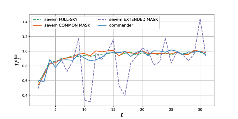
It is possible to note that the commander and both the sevem computed considering full-sky and the Planck common mask are very similar. The sevem computed considering the extended mask is very noisy but follows the behaviour of the one computed with the standard mask. For this reason we apply the last one to the theoretical power spectra.
We correct for these transfer functions the values of theoretical power spectra TE and EE which enter in the equation of NAPS (2.2), (2.5) and (2.6). In the NAPS computed for the sevem dataset we apply the following correction:
| (B.2) | |||||
| (B.3) |
while for the commander dataset
| (B.4) | |||||
| (B.5) |
where is the E-mode transfer function provided for commander by the Planck team.
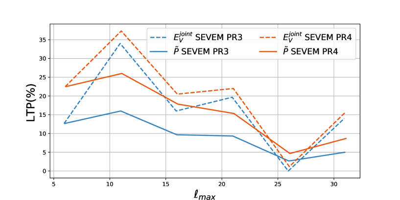
Appendix C Comparison with previous estimator
In this appendix we show the application to latest Planck sevem datasets of the joint estimator for the lack of power developed in [27]. We combined the NAPS and to define the optimal, i.e. with minimum variance, estimator as:
| (C.1) |
with:
| (C.2) | |||||
| (C.3) |
where and are the variance of and respectively, and is their covariance
| (C.4) |
The coefficients and are obtained with the method of the Lagrange multipliers by minimising the variance of , at each , on the constraint . The estimator could be interpreted as a dimensionless normalised mean power, which jointly combines the temperature and polarisation data, with an expectation value of:
| (C.5) |
regardless of the value of .
Now we apply this estimator on the PR3 and PR4 sevem dataset, MC simulations and data, in the harmonic range , considering a constant bin of . Figure 16 displays the computed for the applied on the PR3 (blue solid line) and PR4 (orange solid line) sevem datasets as a function of . Moreover it is also shown the comparison with the computed with both the datasets, PR3 (blue dashed line) and PR4 (orange dashed line) sevem datasets. Both the estimators when applied to the PR3 dataset provide estimates which are less likely accepted in a CDM model than when applied to the PR4 dataset. Moreover, it is interesting to note that the trends of these two estimators are similar, showing peaks and valleys for the same values of .