The Next Generation Deep Extragalactic Exploratory Public Near-Infrared Slitless Survey Epoch 1 (NGDEEP-NISS1): Extra-Galactic Star-formation and Active Galactic Nuclei at 0.5 $<$ z $<$ 3.6

Abstract

The Next Generation Deep Extragalactic Exploratory Public (NGDEEP) survey program was designed specifically to include Near Infrared Slitless Spectroscopic observations (NGDEEP-NISS) to detect multiple emission lines in as many galaxies as possible and across a wide redshift range using the Near Infrared Imager and Slitless Spectrograph (NIRISS). To date, the James Webb Space Telescope (JWST) has observed 50$\%$ of the allocated orbits (Epoch 1) of this program (NGDEEP-NISS1). Using a set of independently developed calibration files designed to deal with a complex combination of overlapping spectra, multiple position angles, and multiple cross filters and grisms, in conjunction with a robust and proven algorithm for quantifying contamination from overlapping dispersed spectra, NGDEEP-NISS1 has achieved a 3$\sigma$ sensitivity limit of 2 $\times$ 10^-18 erg/s/cm². We demonstrate the power of deep wide field slitless spectroscopy (WFSS) to characterize the dust content, star-formation rates, and metallicity ([OIII]/H$\beta$) of galaxies at $1<z<3.5$. Further, we identify the presence of active galactic nuclei (AGN) and infer the mass of their supermassive black holes (SMBHs) using broadened restframe MgII and H$\beta$ emission lines. The spectroscopic results are then compared with the physical properties of galaxies extrapolated from fitting spectral energy distribution (SED) models to photometry alone. The results clearly demonstrate the unique power and efficiency of WFSS at near-infrared wavelengths over other methods to determine the properties of galaxies across a broad range of redshifts.

1 Introduction

A critical component to maximizing surveys of emission line of galaxies is the balance among efficiency, depth, and resolving targets sufficiently to fully characterize their physical properties. Purely photometric surveys may be the most efficient method in terms of depth and sensitivity versus time required, but their accuracy in determining redshifts, dust, metallicity, stellar ages, etc. are highly dependent upon the input models used to match and fit the observed data, the methods and assumptions which go into such modeling, and a sufficient number of filters to properly sample the spectral energy distributions (SEDs) of galaxies. As more filters are used, the efficiency of such surveys lessens. Spectroscopy is the gold standard and should always be used to verify redshifts, and other galaxy properties. However, spectroscopic observations are not without complications. Extracting parameters from objects beyond the local Universe can be extremely time expensive, even with the largest apertures. At wavelengths beyond 0.8 $\mu$m, such observations are further complicated by telluric sky emission and atmospheric absorption, as well as thermal contributions from the sky and instruments at longer near-infrared wavelengths. Further, the nuts and bolts of standard spectroscopic observations, such as slit alignment, constructing multi-object-slit masks to efficiently maximize a survey field, maximizing multi-fiber placement, or the various complexities of integral field unit observations (field of view, wavelength coverage, spectral resolution, etc) can hinder the depth and efficiencies of such observations.

Wide field slitless spectroscopy (WFSS) provides a balance between the limitations of purely photometric surveys and the complexities of standard types of spectroscopic observations. Such techniques are neither new, nor novel (See Pirzkal et al., 2017b, for a brief review). WFSS disperses the light of every object observed in the field of view (FOV), thus eliminating the problems of slit loss, misplaced fibers, etc.. The spectral resolution (R) of WFSS is significantly less than standard spectroscopy (R$\simeq$ 10s-100 versus $>>$ few hundred) but it is sufficient to measure important characteristics beyond just redshift, such as metallicity, dust, and even detect active galactic nuclei (AGN). One downside to WFSS is that spectral contamination can occur from overlapping spectra produced by sources in close proximity to each other, and/or from multiple orders dispersed across the detector. However, with careful planning (e.g. observations taken with different orientations on-sky and/or using orthogonally crossed dispersers) and careful forward modeling of contamination (e.g. EM2D, MAP2D, see Pirzkal & Ryan, 2017; Pirzkal et al., 2018, for details), one can reduce the impacts of spectral contamination. Moving beyond Earth’s atmosphere alleviates the impact of telluric absorption and emission lines and the limitations of limited atmospheric transparency windows in the near-infrared. Observations from the Hubble Space Telescope (HST) are still impacted from Earth glow in certain orientations (Brammer et al., 2014; Pirzkal & Ryan, 2020; Pirzkal et al., 2017b; Simons et al., 2023) and along with the James Webb Telescope (JWST Gardner et al., 2023) may still be affected by thermal contributions from the instruments and telescope itself, but at levels significantly less than ground-based observations.

NGDEEP-NISS1 (The Next Generation Deep Extragalactic Exploratory Public Near-Infrared Slitless Spectroscopic survey 1) follows a legacy of programs using space-based WFSS deep surveys of the $\approx 3^{\prime}\times 3^{\prime}$ Hubble Ultra Deep Field (HUDF, Beckwith et al., 2006), specifically the Grism ACS Program for Extragalactic Science (GRAPES, Pirzkal et al., 2004) the Probing Evolution And Reionization Spectroscopically (PEARS, Pirzkal et al., 2009), which both used the the optical (0.4$\mu$m $<$$\lambda$$<$ 1$\mu$m) Advanced Camera for Surveys (ACS), and later the Faint Infrared Grism Survey (FIGS, Pirzkal et al., 2017b) using the Wide Field Camera 3 (WFC3), with an emphasis on the near-infrared camera, which extended coverage to 1.6$\mu$m. The programs cited above come in addition to WFSS programs that, while shallower, covered larger areas such as WISPS (Atek et al., 2010), 3DHST (Brammer et al., 2012; Momcheva et al., 2016), and CLEAR (Simons et al., 2023). Until the launch of JWST, space-based WFSS surveys at longer wavelengths were not possible. NGDEEP-NISS was designed specifically to take advantage of the capabilities of JWST’s Near Infrared Imager and Slitless Spectrograph (NIRISS Doyon et al., 2023), which covers a wavelength range 1$\mu$m $<$ $\lambda$ $<$ 2.3$\mu$m (using the three cross filters F115W, F150W, and F200W) over a 2′.2 $\times$ 2′.2 FOV, with a spectral resolution of R$\simeq$ 150. The goals of the program include the study of emission line galaxies at higher redshifts, detecting faint emission lines, and leveraging the wide wavelength range to detect multiple emission lines which allows for more robust scientific analysis of galaxy properties such as gas metallicity, the Balmer decrement (internal dust extinction), BPT diagrams (the Baldwin, Phillips & Terlevich star-formation versus AGN diagnostic, Baldwin et al., 1981), among other parameters, for galaxies over the redshift range of 1 $<$ z $<$ 3.5. For a more in-depth overview of NGDEEP, the reader is referred to Bagley et al. (2023). Further, the angular spatial resolution of NIRISS (0.09-0.1″), in combination with four distinct orientations (two orthogonal grisms used at two position angles on the sky) allows for NGDEEP-NISS observations to be used to construct two-dimensional spatial maps of galaxies as a function of wavelength. That is, for each resolved source in the field, one can resolve individual areas of emission beyond the nucleus and map the presence and intensity of star-formation, which helps to further constrain the evolutionary history of these systems.

As of now, exactly half of the NGDEEP-NIRISS observations have been obtained in February 2023, using two grisms but at a single orientation on the sky, and has achieved an average sensitivity of 1.88 $\times$ 10^-18 erg/s/cm² (for a 3$\sigma$ detection, see Table 1 for more details). This paper presents the first look at NGDEEP-NISS1. The goals of this paper are: 1) showcase the quality of the NGDEEP-NISS1 data and how it compares to how pre-launch expectations; 2) show how NGDEEP-NISS1 emission line measurements of extincion and star-formation rates differ from the same properties obtained from fitting spectral energy distributions (SEDs) to photometry alone; and 3) explore the redshift evolution of the population of star forming galaxies at $1<z<3.5$.

All calculations in this paper assume $H_{0}=67.3\ km\ s^{-1}Mpc^{-1}$ and $\Omega_{M}=0.315$, $\Omega_{\Lambda}=0.685$ (Planck Collaboration et al., 2014). All magnitudes are given in the $AB$ system (Oke & Gunn, 1983).

2 Data Reduction and Analysis

2.1 Pipeline and Catalogs

We started by using the rate files STScI (Space Telescope Science Institute) Pipeline Stage 1 products to perform the bias subtraction, dark current correction, and on-the-ramp fitting to produce partially calibrated slope images. The pipeline Stage 2 calwebb_image2 was used for all data, including WFSS observations in order to populate the world coordinate system (WCS) of each image using assign_wcs, and apply the appropriate imaging filter flat-field using flat_field. We used the STScI pipeline version 1.9.4, CRDS version 11.16.20 and the CRDS context file jwst_1041.pmap, which were the most up to date at the time. These steps were performed in order to be able to produce 1D fully calibrated spectra using an implementation of the SBE (Simulation Based Extraction) technique detailed in Pirzkal et al. (2017b) from partially calibrated WFSS observations in units of DN/s.

Part of the process of selecting and extracting WFSS data requires the presence of a field image. This image (or images) is (are) used to match the dispersed light to its source. For the NGDEEP-NISS1 data, four sets of images were used. First, a catalog of source candidates to extract was generated from SExtractor (Bertin & Arnouts, 1996) using an HST CANDELS (Grogin et al., 2011) F160W GOODS-S master mosaic, which was first astrometrically corrected to match the GAIA Data Release 3 (DR3) catalog. See Koekemoer et al. (2011) and Section 2.2 of Leung et al. (2023) for more details regarding its creation. Next, a second set of mosaicked fields were created from the NGDEEP-NISS1 images in each of the F115W, F150W, and F200W filters. These imaging observations were taken during the same pointing of the JWST WFSS observations and represent a 1:1 match between objects and their dispersed light. These mosaics were created using the JWST Level 3 pipeline. However, these were not corrected to match the astrometry from the GAIA DR3 catalog, as this would break the relative alignment between the NGDEEP-NISS imaging and NGDEEP-NISS WFSS data. Instead, sources were detected in each of the individual (F115W, F150W, and F200W) NGDEEP-NISS mosaics. An affine transformation (shift and rotation) was then derived between each mosaic and the HST F160W GOODS-S master mosaic. Thus, the coordinates of any of the pixels in the master moasic could be accurately (to within $<0.1$ pixel) mapped onto the individual NGDEEP-NISS mosaics, and thus by extension, onto the individual WFSS observations.

2.2 Photometry

NIRISS WFSS were used in conjunction with photometry of the HUDF from HST/ACS (F435W, F606W, F775W, F814W, and F850LP filters), HST/WFC3-IR (F105W, F125W, F140W, and F160W filters), and JWST/NIRISS imaging (F115W, F150W, and F200W filters), for a total of 12 bands which span a range of observed wavelengths from 0.4 to 2.5$\mu$m. The analysis and methods for constructing the mosaic images and measuring the photometric data can be found in Leung et al. (2023). The photometric data were used exclusively to calculate stellar masses, star-formation histories, and SEDs. They were also used to determine metallicities, extinction values and dust corrections, and redshifts. These values were then compared to those determined directly from WFSS data. The masses derived from photometry were also used to correct [NII] contamination from ${\rm H\alpha\ \lambda 6565}$ for generating BPT diagrams.

2.3 WFSS Extraction and Calibration

Following the method described in (Pirzkal & Ryan, 2017), the dispersed WFSS observations were fully simulated using the object pixel coordinates from the master mosaic and the pixel level photometry of the individual F115W, F150W, and F200W mosaics: For every galaxy, a defined smooth spectral energy distribution (SED) was generated for each imaging pixel of the galaxy, which could then be dispersed numerically to produce an accurate and smooth simulation of the source in each individual NGDEEP-NISS WFSS dataset. The initial simulations using the official STScI NIRISS WFSS calibration files (based on commissioning data and some Cycle 1 observations) showed large offsets (as much as 2 pixels, or $\approx 90\AA$ in the dispersion direction) between the expected and measured positions of dispersed spectral traces in the observations. These errors were too large to quantitatively and rigorously correct the contamination from overlapping spectra or to produce accurate observed wavelengths of emission lines when using different grisms and cross filters. Further, these errors create spurious features which could be misidentified or misinterpreted as real physical results.

Since NGDEEP-NISS combines multiple spectra, obtained using two cross filters, different grisms, and two orientations on the sky, the official STScI calibration products, with a precision on the order of 1 to 2 pixels, proved inadequate for our needs. Therefore, a new set of calibration files for the NIRISS WFSS mode were derived for the F115W, F150W, and F200W imaging cross filters with the GR150R and G150C grims to bring the calibration uncertainties down to about 0.2 pixel, both in terms of trace location and shape as well as wavelength calibration. This work followed the methodology used to calibrate the HST/WFC3 WFSS mode (See Pirzkal et al., 2016, 2017a, for details). Appendix B provides quantitative comparisons regarding the accuracy achieved from these calibrations, and the improvement in accuracy reached by the NGDEEP-NISS calibration when compared to the STScI NIRISS WFSS calibration. All of the work described in this paper, including simulations and extractions, used the improved NGDEEP-NISS calibrations. These calibrations will be made publicly available as a service to the community.

Similarly to what was done in Pirzkal et al. (2017b), full 2D simulations were used to estimate and subtract the background from individual WFSS observations, and to provide quantitative estimates of the WFSS contamination resulting from overlapping dispersed spectra. First, individual rectified 2D spectra were generated from each observation. Next, these were subsequently combined to produce deep, rectified 2D spectra, from which fully calibrated 1D spectra could be generated using an optimal extraction method closely based on (Horne, 1986). Then, for each source, 6 individual spectra were generated using the GR150R and GR150C grisms, combined with the F115W, F150W, and F200W cross filters. GR150R and GR150C are identical grisms but oriented perpendicularly. Figures 1 and 2 show examples of 2D rectified spectra, as well as the final, calibrated 1D spectra. Multiple emission lines such as ${\rm[OII]\lambda\lambda 3726,3729}$, ${\rm H\beta\ \lambda 4863}$, ${\rm H\alpha\ \lambda 6565+[NII]\lambda\lambda 6550,6585}$, ${\rm[OIII]\ \lambda\lambda 4960,5008}$, are clearly detected in both figures. Spectra of similar quality have been extracted out to z $\sim$ 3.

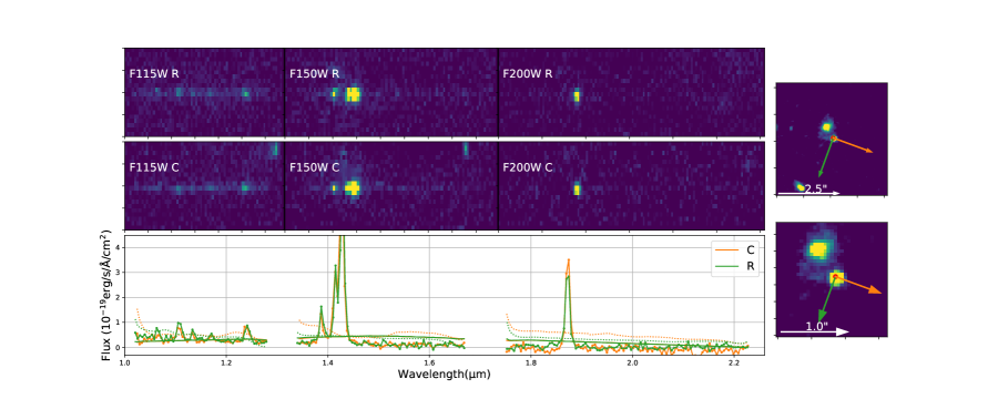
Figure 1: An example spectrum of one of the NGDEEP-NISS1 sources (ID $\#$33273). The rightmost panels show two views of the field image, the top is a larger field of view 5$\arcsec$ $\times$ 5$\arcsec$ arcseconds in size, the bottom is a zoom-in 2$\arcsec$ $\times$ 2$\arcsec$ in size. The color arrows show the directions of the light dispersed by the G150C (orange) and G150R (green) grisms. Prominent emission lines are seen with the F115W, F150W, and F200W cross filters (Rows 1 and 2: left, center, and right, respectively) used in conjunction with the GR150C (Row 1 and in orange in the bottom plot) and GR150R (Row 2 and in green in the bottom plot) NIRISS grisms. This source has a magnitude of $m_{AB,F160W}=24.8$ and is at z=1.85. The dotted lines show the contamination estimates which were subtracted from the observed spectra. The initial models, estimated using photometry, are also plotted (solid smooth lines). No continuum was subtracted from these spectra.

2.4 Emission lines detection and fitting

The final 1D extracted spectra were visually inspected and a set of 144 sources with easily identifiable emission lines (${\rm H\alpha\ \lambda 6565+[NII]\lambda\lambda 6550,6585}$+ ${\rm[SII]\ \lambda\lambda 6718,6733}$, and/or ${\rm[OIII]\ \lambda\lambda 4960,5008}$+${\rm H\beta\ \lambda 4863}$) were selected. The identification and initial fitting of these emission line in the 1D spectra allowed for the determination of accurate spectroscopic redshifts for each of the sources. The line selection was limited to manual identification of ${\rm H\alpha\ \lambda 6565+[NII]\lambda\lambda 6550,6585}$+${\rm[SII]\ \lambda\lambda 6718,6733}$, and/or ${\rm[OIII]\ \lambda\lambda 4960,5008}$+${\rm H\beta\ \lambda 4863}$ lines and their observed wavelengths in the extracted spectra. The requirement for this was that the emission lines should be identifiable in both the GR150R and GR150C grisms. Once a redshift for each source was set, the lines were subsequently fit, and the fluxes of emission lines estimated.

It is important to note that the initial line identifications used to determine redshifts are only a starting point. The excellent spatial resolution of NIRISS WFSS allows for resolved spectra to be measured spatially across resolved or partially-resolved sources. This allows one to detect extra-nuclear emission lines resulting from star-forming regions or outflows potentially related to AGN. As demonstrated in Pirzkal et al. (2018) for HST/WFC3 WFSS, such shifts must be carefully accounted for, including the impact from self-contamination (e.g. multiple emission line sources along the dispersion axis, with each source dispersing light on top of each other). That is, each position angle should be extracted and 1D spectra generated separately. In the case of NIRISS, in addition to each position angle, each orthogonal grism must be treated individually. This can be used to construct spatially resolved 2D spectra of targets when obtaining spectra at multiple position angles and/or orthogonal grisms. Figure 2 shows an example of a spatially resolved target and the resulting G150C and G150R 2D dispersed spectra, along with the 1D spectrum extracted from each grism. Also shown are postage stamp images of the targets at two different fields of view. Overplotted on the postage stamp images are lines showing the dispersion direction for each grism. Since the position of the source of the dispersed light is different in each grism (or contains multiple sources), the resulting spectra will produce an apparent wavelength shift. Further, if an object is resolved, or partially resolved and has any ellipticity, then any differences in the full width at half maximum (FWHM) of the source between the orthogonal grisms will produce a significant shift.

Therefore, all measurements of the emission line fluxes were made by fitting all emission lines simultaneously in each of the 6 available spectra (two orthogonal grisms for each of the three filters). This was done using a single flux value for each emission line, but allowing the FWHM of the lines, and the continuum to vary in each of the 6 spectra. The continuum emission was modelled as a second order polynomial. Finally, in order to account for shifts between the GR150R and GR150C spectra caused by extra-nuclear located emission line regions, a linear offset (in wavelength) between the GR150R and GR150C spectra were included. The GR150R observed wavelengths were used as the fiducial (ths is arbitrary, and the G150C could also be used as the fiducial spectra). A custom line fitting code to perform these measurements were developed using Bilby (Ashton & Talbot, 2021) with the Dynesty (Speagle, 2020) sampler, which are an implementation of Markov-Chain Monte Carlo (MCMC) analysis. This approach leveraged all of the available information which allowed for an estimate of the emission line fluxes’ posteriors, with reliable confidence regions, and realistic error estimates. For the purposes of this paper, all emission lines selected were those with $SNR>2$. Figures 3 and 4 show the final 1D spectra generated from the two orthogonal grisms plotted in each of Figures 1 and 2. Figure 5 shows a stacked image of all the emission lines spectra ($SNR\ >$ 2) discussed in this paper, ordered by redshift.

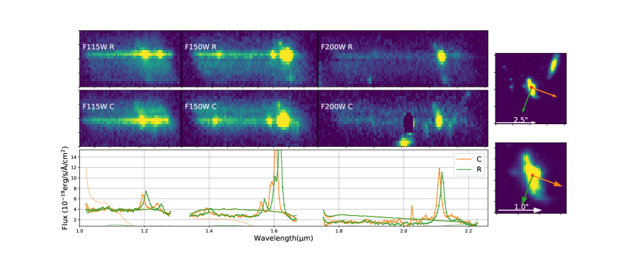
Figure 2: Similar to Figure 1 (colors and lines have the same meaning), however, this spectra of an NGDEEP-NISS1 target (ID$\#$35875) demonstrates the offset between the orthogonal grisms which is due the presence of off-nuclear, spatially resolved star-formation. This offset produces different observed wavelengths being assigned to emission lines in the R and C grisms. Simply combining or averaging the two orthogonal grisms without taking this into account could lead to spurious scientific conclusions. The host galaxy is a $m_{AB,F160W}=22.48$ at z=2.23. The blackened pixels in the bottom dispersed figure represents data masked due to contamination which cannot be corrected.

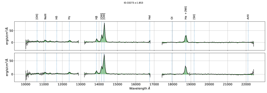
Figure 3: Fits to the continuum and emission lines of the source shown in Figure 1. The measured spectra are shown in black while we show the emission line fits in green. Prominent emission lines are indicated using vertical lines.

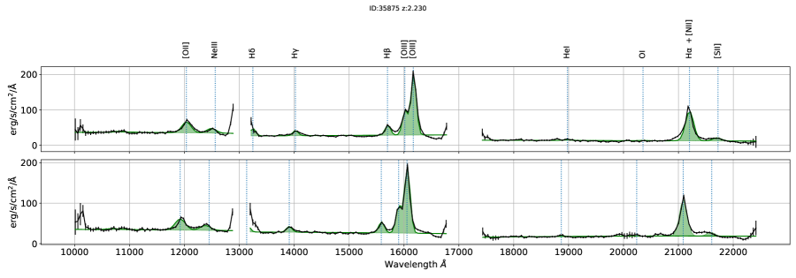
Figure 4: Fits to the continuum and emission lines of the source shown in Figure 2

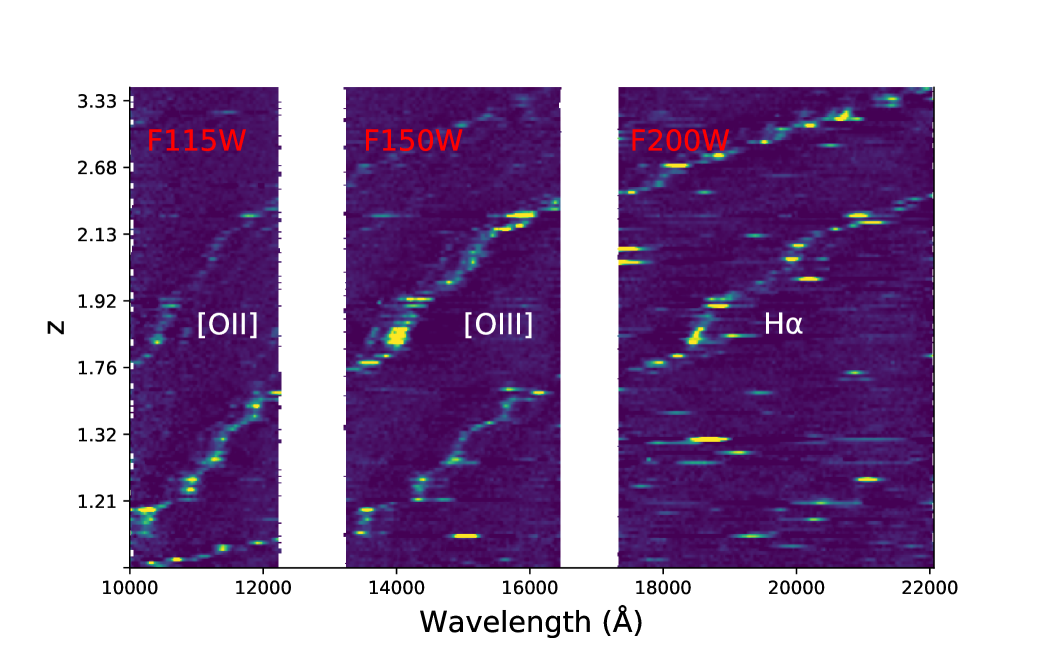
Figure 5: Stacked 1D NGDEEP-NISS1 spectra, ordered as a function of redshift. The [OII], [OIII], and ${\rm H\alpha}$ lines are indicated. Lines other than [OII], [OIII], and ${\rm H\alpha}$ are present in this figure. A list of these lines are presented in Table 2 and will be addressed in more detail in future papers.

3 Results

The results presented here represent the first set of data obtained with NGDEEP-NISS1. The goal of this paper is to present first results, not a comprehensive or in-depth analysis from the data. But more importantly, it is to demonstrate the capabilities of carefully calibrated WFSS data from NIRISS and what physical parameters can be determined from these data. Results are also presented from combining NGDEEP-NISS1 data with ancillary and complimentary photometric data. The NIRISS WFSS data are used exclusively to calculate star-formation rates (SFR), extinction values and dust corrections using the Balmer decrement (e.g. Struve & Schwede, 1931; Baker & Menzel, 1938a; Miller & Mathews, 1972), and of course, redshift determinations. The quality of the NGDEEP-NISS1 data is such, that AGN candidates have been identified via the BPT diagram and another z $\sim$ 3.18 candidate identified from broadened emission lines for which an estimate of the black hole mass has been made. In each sub-section below we detail the various physical parameters which can be extracted from the NGDEEP-NISS1  data and serve as an example of the power of deep NIRISS/WFSS observations with JWST. In all the work shown in this paper, asymmetrical error bars were estimated by using the full posterior distributions of the measured emission line fluxes and the full posteriors were furthermore propagated throughout any computation made in order to derive realistic error estimates.

3.1 Emission Lines Fluxes

Table 1 lists the calculated $3\sigma$ and $5\sigma$ flux limits based on the data shown in Figure 6. On average, NGDEEP-NISS1 reaches down to $1.8\ (3.3)\times 10^{-18}\ erg/s/cm^{2}$ at the $3\ (5)\sigma$ level. Figure 6 also shows the predicted SNR from the 2D simulations (Created as part of the NGDEEP proposal design), as well as from the JWST Exposure Time Calculator (ETC) 2.0 (Adjusted to account for the data having half the depth of our final goal). Overall, NGDEEP-NISS1 matches the pre-launch expectations well, although it is slightly less sensitive in the F115W filter than in the F150W and F200W filters. Table 2 lists the number of emissions lines ($SNR>2$) identified so far in the NGDEEP-NISS1 data as part of this initial sample while Table 4 lists the individual measured emission line fluxes for the current sample. Figure 7 shows the distribution of rest-frame equivalent width for the oxygen and hydrogen lines.

Table 1: NGDEEP-NISS1 Emission Line Flux Limits

Filter	$5\sigma$ flux limit	$3\sigma$ flux limit
	${\rm 10^{-18}\ erg/s/cm^{2}}$	${\rm 10^{-18}\ erg/s/cm^{2}}$
F115W	4.17	2.17
F150W	2.69	1.49
F200W	2.83	1.56
ALL	3.33	1.84

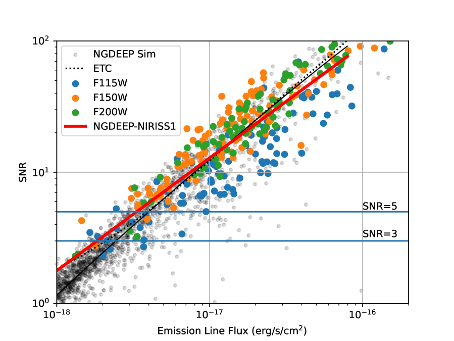
Figure 6: Signal to noise (SNR) of the NGDEEP-NISS1 emission lines as a function of emission line flux. Shown are emission lines detected using the F115W (blue), F150W (orange), and F200W (green) cross filters, as well as a polynomial fit to the data. The F150W and F200W data achieve similar sensitivities, while the F115W data are somewhat noisier. Also plotted are the SNRs of our pre-launch simulated data (black points), the fit to this data (red line). These are then compared with the estimates using the JWST ETC 2.0 (black dotted line).

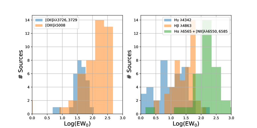
Figure 7: The rest-frame equivalent widths (EW) of the ${\rm[OII]\lambda\lambda 3726,3729}$ and ${\rm[OIII]\ \lambda}$5008 emission lines (Left panel) and of the ${\rm H\alpha\ \lambda 6565+[NII]\lambda\lambda 6550,6585}$, ${\rm H\beta\ \lambda 4863}$, and ${\rm H\gamma\ \lambda 4342}$ emission lines in NGDEEP-NISS1

Table 2: NGDEEP-NISS1 Emission Lines

Line	Number	Average Line Flux
Identified	of Galaxies	${\rm 10^{-18}\ erg/s/cm^{2}}$
${\rm[NeIV]\lambda}$2439	3	6.16 $\pm$ 1.80
${\rm MgII\lambda}$2799	2	15.87 $\pm$ 5.05
${\rm[NeV]\lambda\lambda}$3347	10	2.78 $\pm$ 0.26
${\rm[NeV]\lambda\lambda}$3427	10	2.40 $\pm$ 5.65
${\rm[OII]\lambda\lambda 3726,3729}$	80	7.13 $\pm$ 0.13
${\rm[NeIII]\lambda\lambda}$3869	46	3.03 $\pm$ 0.11
${\rm[NeIII]\lambda\lambda}$3890	28	1.86 $\pm$ 0.07
${\rm[NeIII]\lambda\lambda}$3967	40	2.51 $\pm$ 0.30
${\rm H\gamma\lambda\lambda}$4342	48	3.26 $\pm$ 0.74
${\rm H\beta\ \lambda 4863}$	122	5.24 $\pm$ 0.09
${\rm[OIII]\lambda\lambda}$4960	113	7.84 $\pm$ 0.11
${\rm[OIII]\lambda}$5008	123	21.65 $\pm$ 0.24
${\rm HeI\lambda}$5876	42	2.60 $\pm$ 1.04
${\rm[OI]\lambda\lambda}$6302	28	2.64 $\pm$ 0.52
${\rm H\alpha\ \lambda 6565+[NII]\lambda\lambda 6550,6585}$	104	17.14 $\pm$ 0.28
${\rm[SII]\lambda\lambda}$6718	42	6.91 $\pm$ 0.23
${\rm[SII]\lambda\lambda}$6732	12	4.71 $\pm$ 1.01
${\rm[ArIII]\lambda\lambda}$7753	15	2.26 $\pm$ 2.81
${\rm[SIII]\lambda\lambda}$9069	25	3.35 $\pm$ 0.22
${\rm[SIII]\lambda\lambda}$9531	23	7.21 $\pm$ 0.93
${\rm HeI\lambda}$10830	4	5.54 $\pm$ 1.67
${\rm P\gamma\lambda}$12821	2	4.80 $\pm$ 1.39

Note. — Number of individual emission lines ($\sigma>2$) measured in NGDEEP-NISS1. For each emission line, we also list the mean and standard deviation of the sample of measured fluxes.

3.2 Spectral Energy Distribution Analysis

In addition to using the NGDEEP-NISS1 to determine physical parameters of the sample, the photometric data from HST (ACS and WFC3-IR) and JWST/NRISS observations across 12 filters were used to construct SEDs, and from those, estimates of stellar mass, star-formation histories (ages and rates), and internal extinction from dust. The estimates and associated errors for these properties were determined using Prospector (Johnson et al., 2021) because it provides a convenient way to combine complex stellar population models (Flexible Stellar Population Synthesis, FSPS, Conroy et al., 2009, 2010) with a forward modelling method to constrain physical model parameters. As a check on the results from Propsector, a comparison was made with the same properties obtained from Code Investigating GALaxy Emission (Cigale, Burgarella et al., 2005; Noll et al., 2009; Boquien et al., 2019). While CIGALE is based more on a sparser and finite grid approach to fitting observed photometric measurements to synthetic models, it allowed for a sanity check to be made on the physical parameters derived from photometric SEDs. The only non-photometric data used as an input were the redshifts measured from the WFSS data, and remained fixed during the analysis. Dust content, metallicity, and mass were all allowed to vary. A delayed exponential star formation history was used for this analysis (${\rm SFR(t)\propto t\times e^{-t/\tau}}$). Initially, a Charlot & Fall (2000) dust model was used, although various dust models were tested. Figure 8 shows an example of the photometric SEDs generated from both Prospector and CIGALE for one source in the sample ($m_{AB,F160W}=22.48$ galaxy at z=2.23). The figure shows both the HST and JWST photometry plotted along with the best matched SEDs, and the photometry in the same filters as estimated from the SEDs and input paramters. Figure 8 also shows the maximum a posteriori (MAP) models for the spectra shown in Figure 2.

Tables 6 and 7 lists some of the physical parameters for each of the NGDEEP-NISS galaxies, as determined using Prospector and Cigale, respectively. Both approaches resulted in consistent results but we note that the Prospector derived stellar masses were on average, half of the Cigale estimates. To reflect the true uncertainties in stellar masses, upon which some of our results depend, the average of the Prospector and Cigale stellar mass estimates were used, along with the associated errors from that combination.

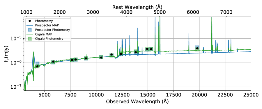
Figure 8: Prospector and Cigale maximum a posteriori fits for the source (ID$\#$35875) shown in Figure 2. The stellar mass of this object is $\approx 1.5\times 10^{10}\ M_{\sun}$ with a stellar age of $\approx 0.178$ Gyr old.

3.3 Emission line Ratios

3.3.1 [NII] contamination of the observed ${\rm H\alpha\ \lambda 6565}$ fluxes

The low resolution of the NIRISS WFSS makes it impossible to separate ${\rm[NII]\ \lambda\lambda 6550,6585}$ emission from nearby ${\rm H\alpha\ \lambda 6565}$. However, one can apply a statistical correction to the 104 measured ${\rm H\alpha\ \lambda 6565+[NII]\lambda\lambda 6550,6585}$ fluxes to derive intrinsic ${\rm H\alpha\ \lambda 6565}$ fluxes. Faisst et al. (2018) derived an empirical correction based on the ${\rm[OIII]\ \lambda\lambda 4960,5008}$, ${\rm H\beta\ \lambda 4863}$, and stellar masses:

$$\begin{gathered}M(Log([NII]/H\alpha),z)=3.696\ \xi+3.236\ \xi^{-1}+0.729\ \xi^{-2}+14.928+0.156(1+z)^{2}\\ \xi=Log([NII]/H\alpha)+0.138-0.042(1+z)^{2}\end{gathered}$$ (1)

This relation was only calibrated up to z=2.5. While statistical in nature, it provides a more nuanced approach than simply assuming a fixed correction (e.g. 30%) or based solely on the observed ${\rm H\alpha\ \lambda 6565+[NII]\lambda\lambda 6550,6585}$ flux since it has now been demonstrated that the amount of ${\rm[NII]\ \lambda\lambda 6550,6585}$ flux is correlated with stellar mass and redshift (Faisst et al., 2018). Using this approach, it is estimated that the contribution of ${\rm[NII]\ \lambda\lambda 6550,6585}$ in the sample is relatively small ($8\pm 11$% of the ${\rm H\alpha\ \lambda 6565}$ flux), as shown in Figure 9. In the rest of this paper, all of the quoted ${\rm H\alpha\ \lambda 6565}$ fluxes have been corrected for [NII] contamination.

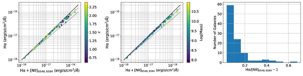
Figure 9: The estimates of the ${\rm H\alpha\ \lambda 6565}$ emission line fluxes after being statistically corrected for ${\rm[NII]\ \lambda\lambda 6550,6585}$ contamination following Faisst et al. (2018). We plot observed versus corrected fluxes, color coded as a function of redshift (mass) in the left (right) panel. The right most panel shows the ${\rm[NII]\ \lambda\lambda 6550,6585}$ contamination as a fraction of ${\rm H\alpha\ \lambda 6565}$ flux.

3.3.2 Correcting for Extinction

One can directly infer the effect of dust for a fraction of the galaxies by comparing the observed Balmer line flux ratios to their canonical values. For the purposes of this paper, Case B is used because it is generally assumed that in typical star-forming regions no Lyman $\alpha$ photons escape, and all are rescattered. A Case B ratio of 2.86 was used for H$\alpha$/H$\beta$ and a ratio of 0.47 was used for H$\gamma$/H$\beta$ assuming a typical electron temperature of $T_{e}=10^{4}K$ and an electron density of $n_{e}=10^{2}\ cm^{-3}$ (Osterbrock, 1989). For the NGDEEP-NISS1 sample, 73 out of 91 sources have $H\alpha$ and $H\beta$ line fluxes consistent with Case B recombination, and 24 out of 45 sources have $H\gamma$ and $H\beta$ emission line fluxes consistent with Case B recombination. Figures 10 and 11 show the measured values of the Balmer line ratios ${\rm H\alpha\ \lambda 6565}$/${\rm H\beta\ \lambda 4863}$ and ${\rm H\gamma\ \lambda 4342}$/${\rm H\beta\ \lambda 4863}$Ṫhis analysis comes with a caveat. While the use of “universal” dust laws (e.g. Calzetti, LMC, SMC, etc) may be somewhat empirically successful in the local Universe, it is far from clear that blanket use of these corrections to all galaxies is warranted or justified (Witt & Gordon, 2000; Salim & Narayanan, 2020, and references therein). Further, the application of such laws to more distant (e.g. z $>>$ 1) objects may not be appropriate either. Although it is likely that many of the objects in the NGDEEP-NISS1 sample are dusty, the distribution of dust (uniform or clumpy), as well as the grain sizes and their composition have yet to be directly characterized or inferred, let alone demonstrated to be the same or similar to galaxies in the local Universe. In this section, calculations of ${\rm A_{V}}$ using the Balmer decrement method are presented purely as a means to compute an average dust content in these objects and to qualitatively compare the sample to previous works as well as to illustrate the limitations of this approach.

As these figures demonstrate, 30% of the 91 sources with a SNR $>2$ for both ${\rm H\alpha\ \lambda 6565}$ and ${\rm H\beta\ \lambda 4863}$ emission lines are observed to have ratios lower than the Case B value of 2.86. Moreover, 47% of sources with ${\rm H\gamma\ \lambda 4342}$ and ${\rm H\beta\ \lambda 4863}$ show ${\rm H\gamma\ \lambda 4342}$/${\rm H\beta\ \lambda 4863}$ values below 0.47. The vast majority of the sample shows ratios incompatible with Case B and any “universal” dust law. This result is not correlated with SNR or other factors related to the quality of the data. For example, Figures 3 and 4 clearly show detected ${\rm H\alpha\ \lambda 6565+[NII]\lambda\lambda 6550,6585}$, ${\rm H\beta\ \lambda 4863}$ , and ${\rm H\gamma\ \lambda 4342}$, but have ${\rm H\alpha\ \lambda 6565}$/${\rm H\beta\ \lambda 4863}$ ratios that are either below 2.86 ($2.74^{+0.04}_{-0.11}$ and $3.15^{+0.03}_{-0.08}$, respectively) or ${\rm H\gamma\ \lambda 4342}$/Hb that are above 0.47 ($+0.56^{0.02}_{-0.06}$ and $0.50^{+0.01}_{-0.02}$,respectively). Figure 12 shows the distribution of Balmer line ratios for 28 sources for which there are $H\alpha$, $H\beta$. and $H\gamma$ emission lines. As this Figure demonstrates, most of these line ratios are observed to be inconsistent with a ”universal” dust law and a Case B photo-ionization model.

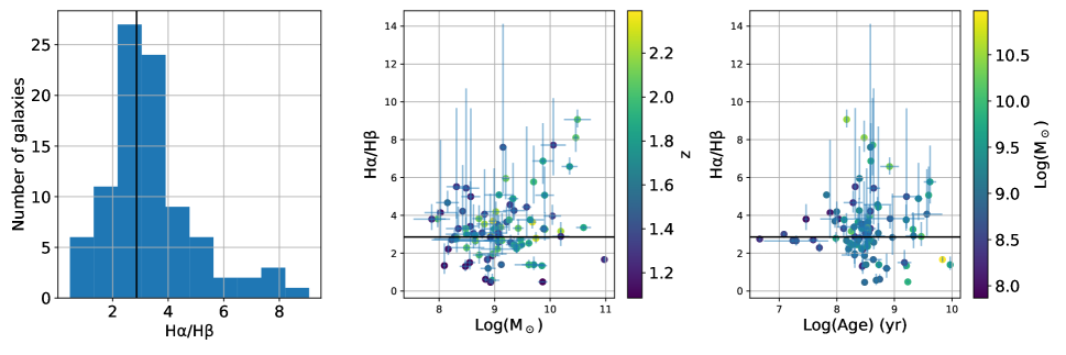
Figure 10: Left Panel: Distribution of ${\rm H\alpha\ \lambda 6565}$/${\rm H\beta\ \lambda 4863}$ lines. Middle Panel: ${\rm H\alpha\ \lambda 6565}$/${\rm H\beta\ \lambda 4863}$ as a function of stellar mass, and color coded by redshift. Right Panel: ${\rm H\alpha\ \lambda 6565}$/${\rm H\beta\ \lambda 4863}$ as a function of stellar ages, and color coded by stellar mass. We show the canonical Case B line ratio in all panels using a solid black line at a value of 2.86.

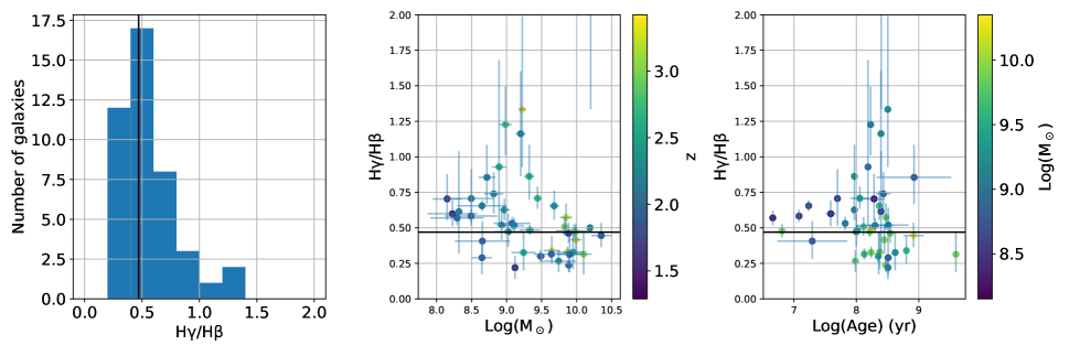
Figure 11: Left Panel: Distribution of ${\rm H\gamma\ \lambda 4342}$/${\rm H\beta\ \lambda 4863}$ lines. Middle Panel: ${\rm H\gamma\ \lambda 4342}$/${\rm H\beta\ \lambda 4863}$ as a function of stellar mass, and color coded by redshift. Right Panel: ${\rm H\gamma\ \lambda 4342}$/${\rm H\beta\ \lambda 4863}$  as a function of stellar ages, and color coded by stellar mass. We show the canonical Case B line ratio in all panels using a solid black line at a value of 0.47.

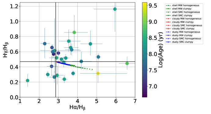
Figure 12: Values of the Balmer line ratios ${\rm H\alpha\ \lambda 6565}$/${\rm H\beta\ \lambda 4863}$ and ${\rm H\gamma\ \lambda 4342}$/${\rm H\beta\ \lambda 4863}$ for the sample of NGDEEP-NISS1 galaxies with measured line fluxes for these three emissions. We also plot line ratios for these emission lines when applying a variety of ”universal” dust laws with values of $0<\tau_{V}<2$, taken from Witt & Gordon (2000), and which include different dust geometries.

For objects which appear to be consistent with Case B recombination, one can use the relations from Osterbrock (1989) to estimate the amount of extinction in the 64 galaxies using the observed ${\rm H\beta\ \lambda 4863}$ line fluxes and the estimates of the intrinsic ${\rm H\alpha\ \lambda 6565}$ line fluxes as described in the previous Section, as well as the 24 galaxies with ${\rm H\beta\ \lambda 4863}$4861 and $H\gamma\ \lambda 4341$ line fluxes. The C00 extinction curve and the equations were used (Domínguez et al., 2013):

$$A_{\lambda}=\kappa(\lambda)E(B-V)$$ (2)

with

$$E(B-V)={2.5\over{\kappa(\lambda_{H\beta})-\kappa(\lambda_{H\alpha})}}Log[{(H\alpha/H\beta)_{obs}\over 2.86}]$$ (3)

or

$$E(B-V)={2.5\over{\kappa(\lambda_{H\beta})-\kappa(\lambda_{H\gamma})}}Log[{(H\gamma/H\beta)_{obs}\over 0.47}]$$ (4)

and for the adopted C00 extinction curve ($\kappa(\lambda)$),

$$\kappa(V)=R_{V}=4.05\pm 0.8\\$$ (5)

$${2.5\over{\kappa(\lambda_{H\beta})-\kappa(\lambda_{H\alpha})}}=1.91\pm 1.66\\$$ (6)

$${2.5\over{\kappa(\lambda_{H\beta})-\kappa(\lambda_{H\gamma})}}=-4.76\pm 10.3\\$$ (7)

The left panel of Figure 13 shows the distribution of empirically derived ${\rm A_{V}}$ values using the Balmer decrement method. The center panel of this Figure shows ${\rm A_{V}}$ as a function of stellar mass (as estimated using Prospector and Cigale, see Section 3.2 for details) color coded by redshift. The right panel compares ${\rm A_{V}}$ with stellar ages (as estimated using Prospector and Cigale) and color coded by mass. The figure shows no evidence for a dependence of ${\rm A_{V}}$ on stellar mass. However, the right panel does show a correlation between ${\rm A_{V}}$ and stellar ages, with increased ${\rm A_{V}}$ as age increases.

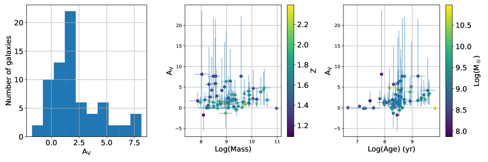
Figure 13: Left Panel: Extinction (${\rm A_{V}}$) values derived using our estimated ${\rm H\alpha\ \lambda 6565}$ and measured ${\rm H\beta\ \lambda 4863}$  assuming a Case B scenario and an intrinsic Balmer line ratio of 2.86. Middle Panel: ${\rm A_{V}}$ as a function of stellar mass, color coded by redshift. Right Panel: ${\rm A_{V}}$ as a function of stellar ages, color coded by stellar mass.

Figure 14 shows a comparison between ${\rm A_{V}}$ measured from the Balmer ratio with ${\rm A_{V}}$ inferred from SED fitting as explained in Section 3.2. The latter are expected to be representative of the dust content in the host galaxies as a whole, while the estimates derived using emission line flux measurements are for the spectroscopically identified star forming regions. Further, Figure 14 shows smaller values of ${\rm A_{V}}$ for star forming regions measured using the Balmer lines than for the host galaxies as a whole (using Prospector). Quantitatively, the difference is $\frac{{{\rm A_{V}}}(SED)}{{{\rm A_{V}}}({{\rm H\alpha\ \lambda 6565}}/{{\rm H\beta\ \lambda 4863}})}=0.59^{+0.05}_{-0.04}$ (when only considering the 19 objects with $\sigma>2$ Balmer decrement derived values of ${\rm A_{V}}$). A similar result was demonstrated by Papovich et al. (2022). In the rest of this paper, all of the emission line fluxes quoted are dust corrected based on the spectroscopic estimates of ${\rm A_{V}}$ (where available). For objects without usable Balmer lines, or those that clearly violate Case B, the Prospector derived values of ${\rm A_{V}}$ are used and corrected by the factor $0.59^{+0.05}_{-0.04}$.

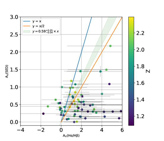
Figure 14: Balmer decrement derived estimates of ${\rm A_{V}}$, indicative of the dust content in individual star forming regions, versus photometry derived values of ${\rm A_{V}}$  indicative of the dust content of the galaxies as a whole, color coded by redshift. We observe that $\frac{A_{V}(SED)}{{{\rm A_{V}}}({{\rm H\alpha\ \lambda 6565}}/{{\rm H\beta\ \lambda 4863}})}=0.59^{+0.05}_{-0.04}$ .

3.4 Star Formation Rates

The instantaneous star formation rates of galaxies in the sample were estimated directly from the dust corrected ${\rm H\alpha\ \lambda 6565}$ emission line fluxes (Kennicutt & Evans, 2012). As shown in Figure 15, the NGDEEP-NISS1 galaxies are typically forming stars at a rate of 0.1 to 1 ${\rm M_{\sun}/yr}$. The star formation rates derived using Prospector with the photometric measurements (${\rm SFR_{SED}}$) are compared to the star formation rates derived directly from the WFSS. Figure 15 shows these two estimates color coded by stellar mass (left panel) and redshift (right panel). The two sets of estimates are consistent between the approaches. 15 shows that many values are roughly consistent (to within a factor $\simeq$ 2), however the Prospector estimated SFR appear to be significantly over-estimated for sources at z $\gtrapprox$ 1.6. Figure 15 also shows linear fits of ${\rm SFR_{SED}}$ vs ${\rm SFR_{H\alpha}}$. There is no strong trend detected as a function of stellar mass as shown in Figure 16.

Figure 16 shows the Whitaker et al. (2012) SFR-Mass relations computed at z=1 and z=2 using photometric measurements from the NEWFIRM Medium-Band Survey. The NGDEEP-NISS1 sample are also plotted. However, NGDEEP-NISS1 achieves fainter emission line flux sensitivity, and thus extends down to lower SFR and smaller stellar masses. Figure 16 demonstrates that most of the NGDEEP-NISS1 objects fall well below the relation derived for z=1.75. yet the median redshift of the 51 NGDEEP-NISS1 objects plotted is $\approx 1.72\pm 0.39$. We derive a relation between SFR and stellar mass with a slope of $0.71\pm 0.03$ over the mass range of $10^{7}<M_{\sun}<10^{11}$ using only the NGDEEP-NISS1. In comparison, the Whitaker et al. (2012) relation predicts slopes between 0.39 and 0.55 over the redshift ranges shown and for masses $>5\times 10^{9}\ M_{\sun}$ .

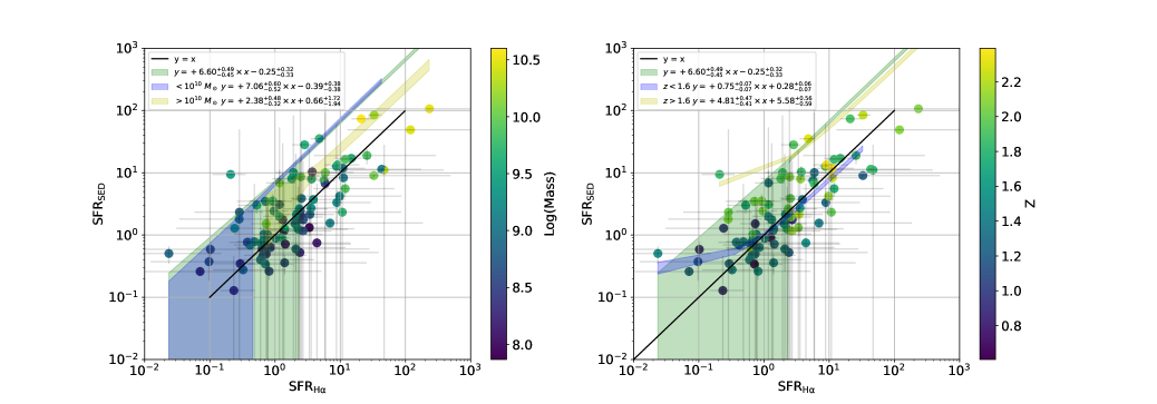
Figure 15: Star formation rates as estimated using broad band photometry with Prospector versus our de-reddened, ${\rm[NII]\ \lambda\lambda 6550,6585}$ decontaminated ${\rm H\alpha\ \lambda 6565}$ results. Larger points are used for objects that were dust corrected using the Balmer decrement. The left panel shows measurements color coded by mass while the right panel shows them color coded by redshift.

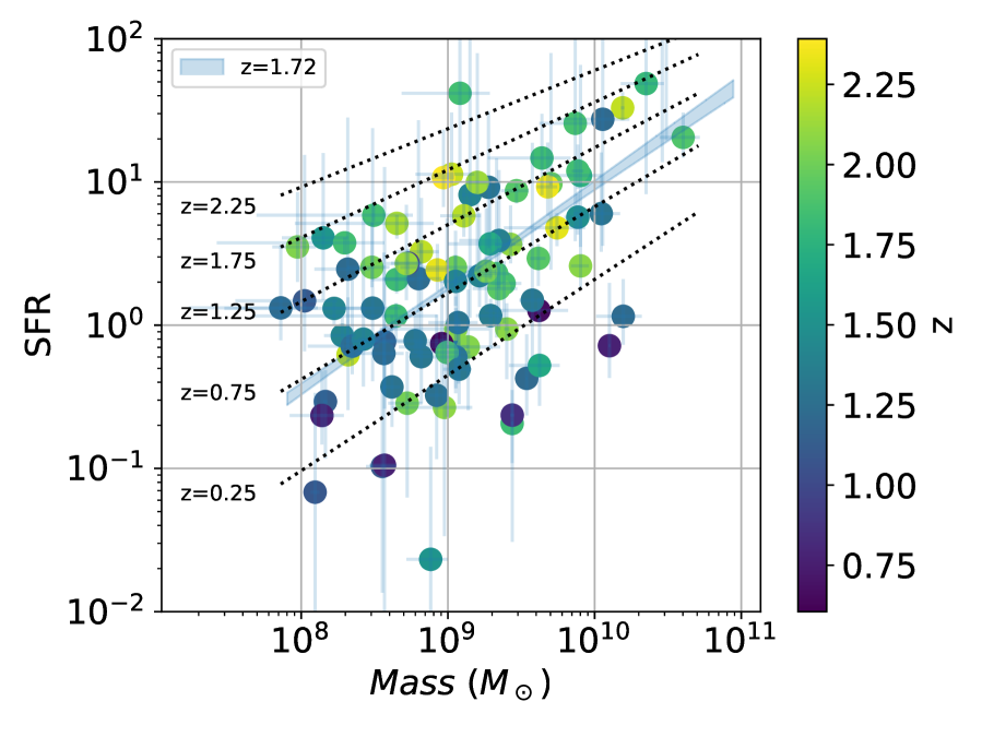
Figure 16: The NGDEEP-NISS1 star formation rate estimates as a function of stellar mass. Plotted in the figure are relations from Whitaker et al. (2012), derived from the NEWFIRM Medium-Band Survey are also shown. A linear fit and its 68% confidence region for the NGDEEP-NISS1 sample (51 sources at $z=1.72\pm 0.29$) is shown in blue. The NGDEEP-NISS1 data have a median redshift of z$\simeq$ 1.72$\pm$0.39 but fall well below the z$=$1.75 relation from Whitaker et al. (2012).

3.5 [OIII]/$H\beta$

Another interesting diagnostic enabled by deep spectroscopy is the ${\rm[OIII]\ \lambda\lambda 4960,5008}$/${\rm H\beta\ \lambda 4863}$ or ${\rm[OIII]\ \lambda}$5008/${\rm H\beta\ \lambda 4863}$  ratio. This has long been used (Baldwin et al., 1981) to separate normal galaxies with HII star forming regions, planetary nebulae, and galaxies that are strongly photo-ionized, either by an active galactic nucleus or from ionizing shocks produced by massive young stars. As shown in Kewley et al. (2013), the ${\rm[OIII]\ \lambda}$5008/${\rm H\beta\ \lambda 4863}$ ratio of star forming galaxies increases as a function of redshift, and is typically greater than 0.6 at $z>1.5$. NGDEEP-NISS1 allows us to examine the ${\rm[OIII]\ \lambda}$5008/${\rm H\beta\ \lambda 4863}$ ratio at higher redshifts, up to, and beyond Cosmic Noon ($z\approx 2$). Nominally, one could use the R23 method (e.g. Pagel et al., 1979; Pagel & Edmunds, 1981) to estimate the gas metallicity of some of our sources, this method uses emission line fluxes over a wavelength range that spans 0.3 to 0.5 $\mu m$. R23 therefore is more sensitive to dust corrections, whereas the ${\rm[OIII]\ \lambda\lambda 4960,5008}$/${\rm H\beta\ \lambda 4863}$ or ${\rm[OIII]\ \lambda}$5008/${\rm H\beta\ \lambda 4863}$ are relatively close in wavelength and hence significantly less affected by variations in dust.

Figure 17 shows the NGDEEP-NISS1 values of ${\rm[OIII]\ \lambda}$5008/${\rm H\beta\ \lambda 4863}$ with $\sigma>2$ as a function of redshift. Also plotted are the shallower measurements obtained from archival WFC3 G102 and G141 data for comparison (Pirzkal et al., 2018, Pirzkal et al., in prep), also restricted to $\sigma>2$ and which are in good agreement with our new JWST observations but cover the lower redshift range of $0.8<z<2$. Using the NGDEEP-NISS1 measurements, we detect a significant increase in the ${\rm[OIII]\ \lambda}$5008/${\rm H\beta\ \lambda 4863}$ line ratio as a function of redshift. Using this, a linear fit was made to the data. The fit (including accounting for all errors), between $1<z<3.5$ is: $Log(\frac{[OIII]}{H\beta})=0.09^{+0.01}_{-0.01}\times z+0.49^{+0.01}_{-0.01}$. This corresponds to an average increase of the [OIII] to $H\beta$ line flux ratio of nearly 23% per unit redshift (i.e. 1–2 Gyr).

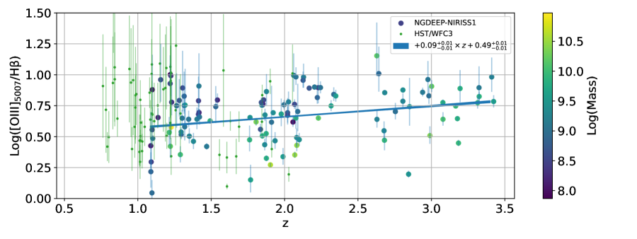
Figure 17: NGDEEP-NISS1 ${\rm[OIII]\ \lambda}$5008/${\rm H\beta\ \lambda 4863}$ as a function of redshift shown, color coded by stellar mass. We show the distribution from the lower redshift but noisier HST/WFC3 G102 and G141 measurements in green. A linear fit to the NGDEEP-NISS1 data and its 68% confidence region are shown in blue.

3.6 BPT

Cross correlating the master source catalog to the Luo et al. (2017) Chandra 7Ms X-ray catalog, four of the NGDEEP-NISS1 sources (IDs $\#$27914, 28858,30372, 32038) are detected in the X-ray by Luo et al. (2017) with X-ray luminosities of $2.71\times 10^{42},5.69\times 10^{41},6.15\times 10^{41},1.01\times 10^{44}$ erg/s, respectively. Sources 28858 and 32038 are identified as AGN dominated, while the other two sources are characterized as star-forming dominated galaxies.

While individual, resolved measurements of the [NII] line fluxes for the NGDEEP-NISS1 galaxies are not possible due to the limitations of the NIRISS spectral resolution, we can use the statistically based ${\rm H\alpha\ \lambda 6565}$/${\rm[NII]\ \lambda}$6584-to-mass relation from Faisst et al. (2018) (see Section 3.3.1), combined with the stellar mass estimates derived from the SED fitting. Using the redshift dependent relation of Kewley et al. (2013):

$$Log([OIII]/H\beta)=\frac{0.61}{Log([NII]/H\alpha)-0.02-0.1833\times z)}+1.2+0.03\times z$$ (8)

while using Equation 1 to estimate the corrected $Log([NII]/H\alpha$) from the stellar mass estimates, NGDEEP-NISS1 sources with measured ${\rm[OIII]\ \lambda}$5008/${\rm H\beta\ \lambda 4863}$ line fluxes are plotted on a BPT diagram shown in Figure 18. This figure shows both a typical BPT diagram (left panel) and and a version which uses stellar mass in place of $Log([NII]/H\alpha$) (right panel) and includes all sources for which there is stellar mass estimate. The right panel in 18 is similar to the Mass Excitation (MEx) diagnostic developed in Juneau et al. (2011), which is applicable to sources out to z $\simeq$ 1 and Juneau et al. (2014), which extended the relation to z $\simeq$ 2. The sources plotted in 18 are limited to objects at $z<2.5$  due to the redshift limitations of the computed lines from Kewley et al. (2013), as well as the redshift upper limits for the correction from Faisst et al. (2018).

Three (IDs $\#$ 27914, 28858, 30372) of the four known X-ray sources are plotted on the left panel of Figure 18. The fourth know X-ray source (32038) is at z $=$ 3.18, which places ${{\rm H\alpha\ \lambda 6565}}$ beyond the spectroscopic limits of the NGDEEP-NISS1 sample. We note the two known X-ray sources identified as star formaing galaxies in Luo et al. (2017) also reside in the star forming region of the BPT diagram, while the known AGN (ID $\#$ 28858) is also identified as AGN dominated.

The NGDEEP-NISS1 spectra of the fourth source (ID $\#$ 32038), show the hallmarks of an AGN dominated object. ${\rm H\beta\ \lambda 4863}$ and MgII emission lines are not only detected, but appear significantly broader than the other emission lines visible in the spectra of this source. We note that there is no shift in the observed wavelengths of the emission lines when observed with the GR150R and GR150C grisms and that the physical source of the emission is therefore located at the center of the source, as determined by SExtractor. The ${\rm H\beta\ \lambda 4863}$ line has a measured FWHM of $92\pm 3.4\AA$ for the average of the GR150R and GR150C grisms. The average FWHM of the ${\rm[OIII]\ \lambda}$5008 line is $46\pm 0.94\AA$, which is very close to the nominal resolution of the NIRISS grisms. This corresponds to a dispersion velocity of $1191\pm 57\ km/s$, consistent with what would be expected from an AGN. Taking the measured F200W flux of $1.816\pm 0.023\ \mu Jy$, or a non-dust corrected luminosity of $9.91\pm 0.13\times 10^{44}\ erg/s$, and using the relation from Wang et al. (2009), leads to a black hole mass estimate of $1.71\pm 0.63\times 10^{8}\ M_{\sun}$. Using the MgII line, which shows a broadened profile of $2259\pm 24\ km/s$, a line luminosity of $8.94\pm 0.11\times 10^{44}erg/s$ and a F115W flux of $964\pm 24\mu Jy$ produces a black hole mass estimate of $1.38\pm 1.02\times 10^{8}\ M_{\sun}$. Due to the lack of ${\rm H\alpha\ \lambda 6565}$ (due to redshift) and the absence of detectable ${\rm H\gamma\ \lambda 4342}$ emission, a dust correction cannot be applied, therefore the black hole mass estimates are taken as a lower limit. A full spectrum of this source, combining the GR150R and GR150C spectra, is shown in Figure 19.

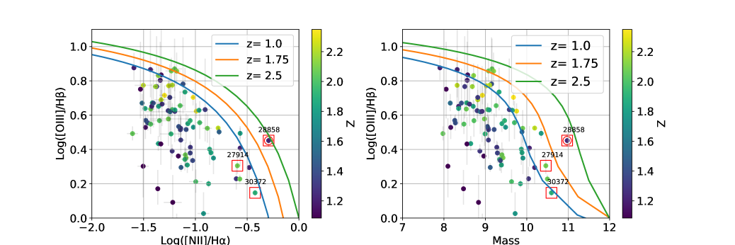
Figure 18: NGDEEP-NISS1 BPT Diagram where we use the Faisst et al. (2018) statistical relation between stellar mass and [NII]/H$\alpha$ ratio (Left Panel) and simply as a function of stellar mass (Right Panel), for NGDEEP-NISS1 sources at $z<2.5$. Previously known X-ray sources from Luo et al. (2017) are marked using red squares. Objects from NGDEEP-NISS1 which are a above the relation of Kewley et al. (2013), computed at their individual redshifts are marked using red circles. The three colored lines are the Kewley et al. (2013) computed at the redshifts of 1.0, 1.75, and 2.5.

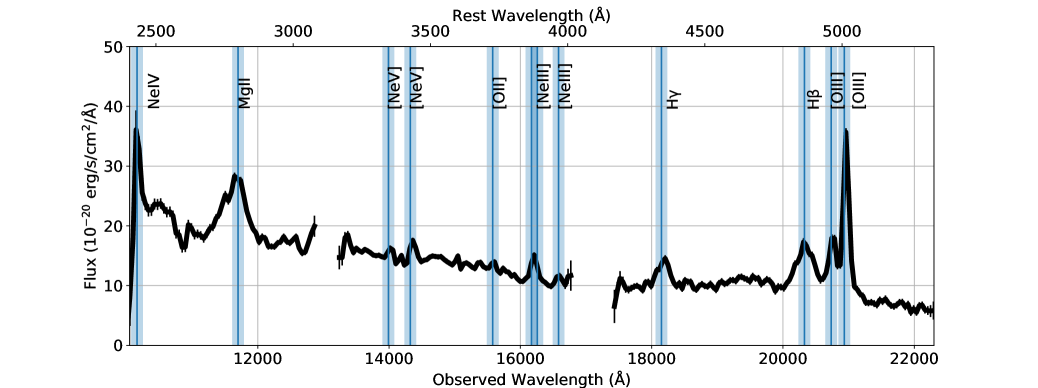
Figure 19: NGDEEP-NISS1 spectrum of source 32038, an AGN dominated galaxy at z=3.18. This source is a known X-ray emitter (Luo et al., 2017) and NGDEEP-NISS1 shows that its MgII and H$\beta$ emission lines are significantly broadened. This object is not shown in Figure 18 as we do not have an ${\rm H\alpha\ \lambda 6565}$ flux for this source. We estimate an outflow velocity of 2000km/s for this source and derive a central black hole mass of $\approx 10^{8}\ M_{\odot}$.

4 Conclusion & Discussion

This work demonstrates a first look at the extracted NIRISS WFSS spectra obtained as part of the NGDEEP-NISS project. Although only half of the allocated observations have been obtained, the results confirm the power of JWST in conjunction with NIRISS WFSS to probe the characteristics of emission line galaxies out to moderate redshifts, including leveraging the improved spectral resolution which allows for the detection of AGN and obtaining mass estimates of SMBHs at z $>$ 3. The paper presents two distinct sets of results. The first, presents an analysis and demonstration of the need for careful extraction, calibration, and analysis of NIRISS WFSS data as outlined in 2.3 and with additional details provided in Appendix B. These results show that the improved calibrations can obtain an accuracy of better than 0.25 pixels for the geometric trace and 10$\AA$ or better for the wavelength calibration (equivalent to one-quarter of a resolution element, on average) regardless of location of the dispersed objects within the field of view. The standard calibration files produce errors 2-3 pixels along the trace, and $\simeq$ 90-120$\AA$ in wavelength-space. Further, this paper establishes a methodology for using these improved calibrations to avoid potential pitfalls when dealing with resolved or partially resolved objects by taking into account the inherent differences in the properties of the GR150C and GR150R grisms. As shown in 3, a number of the scientific results, such as detecting individual star-forming regions within galaxies at z $>$ 1, or obtaining direct mass estimates for a SMBH at z $>$ 3, could not be achieved without the factor of 5-10$\times$ improvement from these new calibrations and methods. Appendix B further quantitatively demonstrates these improvements. As a service to the community, these calibration files are made publicly available and it is hoped that the details provided here will be useful for improving the data products produced from previous and future NIRISS WFSS observations.

The second set of results presented in this paper focus on the science which can be achieved with the NIRISS WFSS observations. The improved spectral and spatial resolution obtained from the G150R and G150C grisms have made it possible to detect multiple emission lines not only from a single galaxy, but from multiple positions within galaxies. The WFSS observations have been used to: characterize star-formation rates, estimate dust corrections using the Balmer decrement, demonstrate a redshift evolution in the ratio of ${\rm[OIII]\ \lambda}$5008/${\rm H\beta\ \lambda 4863}$  compare the correlation of SFR with stellar mass over redshift between NGDEEP-NISS1 other surveys, and ascertain whether the emission line galaxies in the sample are star-formation or AGN dominated using BPT and MEx diagnostics. The last result demonstrates a particularly useful survey and diagnostic power of the NIRISS WFSS data, namely that the instrument has sufficient spectral resolution to detect the presence of AGN and estimate the masses of SMBHs at sensitivies and redshifts beyond what has previously been possible. Further, the paper has demonstrated the power of WFSS observations relative to using photometry alone to constrain the physical parameters of galaxies.

While a number of results shown in the paper have either been consistent with similar works at lower redshift, or at least demonstrated similar correlations, but with scale and depth differences (e.g. SFR vs stellar mass), one interesting result raises questions about the efficacy of certain assumptions. As noted in 3.3.2, the use of the Balmer decrement to constrain and correct for the presence of dust has produced a significant number of sources which appear to violate Case B recombination. Some first hints of this were seen in Matharu et al. (2023). While there exist a number of possible explanations for such violations, one possibility, which has been raised in other surveys such as MOSDEF (Shapley et al., 2022), early release science results from NIRISS (Matharu et al., 2023) etc, is poor signal to noise or significant errors in measuring the fluxes of ${\rm H\alpha\ \lambda 6565}$  ${\rm H\beta\ \lambda 4863}$  etc. Although NGDEEP-NISS has only obtained half of its allocated observations, the SNR of objects which violate Case B are significantly high (e.g. SNR $>$ 10-20). For example, Source 36292, a $z=2.17$ galaxy with a Prospector estimated stellar age of a few million years and a mass of $10^{8}M_{\odot}$  for example, has ${\rm H\alpha\ \lambda 6565+[NII]\lambda\lambda 6550,6585}$, ${\rm H\beta\ \lambda 4863}$, and and ${\rm H\gamma\ \lambda 4342}$ emission lines with SNR of 54, 30, and 19, respectively. These lines are well detected in both GR150R and GR150C and yet result in a ratio of ${\rm H\alpha\ \lambda 6565}$/ ${\rm H\beta\ \lambda 4863}$ of $2.67\pm 0.1$ and ${\rm H\gamma\ \lambda 4342}$/ ${\rm H\beta\ \lambda 4863}$ of $0.65\pm 0.04$.

Another explanation presented in previous works, is to apply an absorption correction to the values of ${\rm H\alpha\ \lambda 6565}$  ${\rm H\beta\ \lambda 4863}$  ${\rm H\gamma\ \lambda 4342}$  etc. The assumption is that in addition to the star-forming regions, there exists a significant (luminosity weighted) stellar population which exhibit Balmer absorption lines. When viewed along the line of sight, these absorption lines contaminate the measured emission lines. Since the spectral resolution of the NIRISS observations are either too poor to detect the absorption lines, or the absorption lines are too faint to be detected relative to the already faint continuum, a emperical correction (e.g. Groves et al., 2012) should be applied to the measured values. It is usually assumed that Balmer absorption should remain very low for stellar population that are less than 1 Gyr old. Yet, galaxies in the NGDEEP-NISS1 sample typically have stellar ages that are only a few hundred million years (see 10 and 11, Source 36292 as noted above).

This suggests that the cause of the violations is more likely to be related to the physical nature of the galaxies themselves. We may be witnessing scenarios in which neither Case A, nor Case B are appropriate to use for dust corrections. Modified versions of Case A and B, namely Case C or Case D (Baker & Menzel, 1938b; Ferland, 1999; Luridiana et al., 2009; Scarlata, 2023), in which the assumption is that neither all of Lyman $\alpha$ photons escape nor are all absorbed. Case C and D suggest that HII regions may contain non-uniformly distributed dust which further scatters and absorbs photons. Such an analysis is deferred to subsequent papers, but we raise the possibility that Case C or Case D may be more appropriate for galaxies with formation histories unlike those in the local Universe. The second epoch of NGDEEP-NISS with the resulting deeper data, and addition of two more position angles should help examine in more details in a follow up paper. Full forward modeling 2D maps will allow us to determine whether there are significant morphological issues in the host galaxies that affect how we currently measure our emission line fluxes.

Appendix A Tables

=2in

Table 3: Dust and contamination corrected emission lines and spectroscopically derived properties

ID	z	H$\alpha$	H$\beta$	[OIII]$\lambda\lambda 4960$	OIII$\lambda\lambda 5008$	[OII]	E(B-V)	Av	SFR(H$\alpha$)
		$10^{-19}erg/s/cm^{2}$	$10^{-19}erg/s/cm^{2}$	$10^{-19}erg/s/cm^{2}$	$10^{-19}erg/s/cm^{2}$	$10^{-19}erg/s/cm^{2}$	mag	mag	M${}_{\sun}/yr$
26465	1.30	$177.76^{+4.73}_{-4.64}$	$107.06^{+8.45}_{-8.30}$		$351.54^{+12.17}_{-12.45}$		$0.06^{+0.02}_{-0.02}$	$6.38^{+12.29}_{-5.46}$	$1.18^{+0.12}_{-0.09}$
27581	2.68		$38.70^{+7.53}_{-7.00}$	$48.99^{+6.37}_{-6.21}$	$114.52^{+7.02}_{-7.03}$	$69.83^{+5.25}_{-5.29}$	$0.58^{+0.65}_{-0.52}$	$6.49^{+7.72}_{-4.56}$
27914	2.08	$537.91^{+8.29}_{-8.21}$	$66.43^{+6.49}_{-6.66}$	$39.00^{+6.55}_{-7.20}$	$178.28^{+9.53}_{-9.00}$	$199.36^{+13.36}_{-14.48}$	$0.90^{+0.76}_{-0.79}$	$2.86^{+6.37}_{-2.49}$	$119.82^{+1456.31}_{-106.85}$
28858	1.23	$374.29^{+6.58}_{-6.45}$	$225.31^{+19.59}_{-19.36}$		$850.80^{+25.45}_{-26.59}$		$0.22^{+0.05}_{-0.05}$	$0.33^{+0.56}_{-0.25}$	$3.47^{+0.90}_{-0.61}$
29659	3.32		$15.30^{+4.87}_{-4.97}$	$41.61^{+5.13}_{-4.81}$	$120.45^{+6.50}_{-6.54}$	$40.43^{+6.41}_{-5.87}$	$0.23^{+0.59}_{-0.26}$	$0.03^{+0.14}_{-0.11}$
30372	1.90	$1000.27^{+6.64}_{-7.05}$	$298.01^{+9.49}_{-9.63}$	$364.01^{+12.06}_{-12.02}$	$557.62^{+11.71}_{-11.98}$	$587.63^{+19.58}_{-21.52}$	$0.13^{+0.13}_{-0.12}$		$21.00^{+10.32}_{-6.21}$
32038	3.18		$109.10^{+5.62}_{-5.87}$	$121.77^{+5.25}_{-5.34}$	$306.02^{+6.11}_{-6.06}$	$14.55^{+3.47}_{-3.40}$	$-0.08^{+0.08}_{-0.14}$	$7.64^{+14.18}_{-5.58}$
33017	2.07	$89.55^{+5.57}_{-5.52}$	$39.15^{+3.42}_{-3.46}$	$93.75^{+3.51}_{-3.40}$	$225.49^{+4.21}_{-4.32}$	$21.39^{+7.44}_{-7.10}$	$0.21^{+0.04}_{-0.04}$	$1.35^{+1.68}_{-0.98}$	$2.90^{+0.74}_{-0.52}$
33273	1.85	$300.78^{+5.58}_{-5.58}$	$109.43^{+3.41}_{-3.36}$	$254.58^{+3.61}_{-3.59}$	$635.79^{+4.34}_{-4.45}$	$31.22^{+7.65}_{-7.50}$	$-0.02^{+0.03}_{-0.06}$		$3.73^{+0.35}_{-0.59}$
34323	1.09	$150.39^{+6.25}_{-5.91}$	$115.98^{+26.64}_{-25.01}$	$68.20^{+10.34}_{-12.06}$	$228.41^{+14.64}_{-12.24}$		$0.01^{+0.01}_{-0.01}$	$-2.65^{+1.99}_{-2.83}$	$0.56^{+0.03}_{-0.02}$
34389	1.09	$48.72^{+7.69}_{-6.08}$	$79.74^{+23.78}_{-23.18}$	$38.24^{+15.68}_{-16.05}$	$130.96^{+17.68}_{-17.07}$		$0.00^{+0.00}_{-0.00}$	$5.88^{+11.07}_{-4.82}$	$0.18^{+0.03}_{-0.02}$
35250	1.69	$28.79^{+9.44}_{-9.15}$					$0.19^{+0.24}_{-0.18}$	$-2.17^{+1.64}_{-2.18}$	$0.52^{+0.66}_{-0.25}$
35875	2.23	$1239.91^{+12.07}_{-12.44}$	$392.48^{+7.57}_{-7.76}$	$842.90^{+8.00}_{-7.91}$	$1752.73^{+9.77}_{-9.49}$	$633.01^{+16.36}_{-16.24}$	$0.08^{+0.08}_{-0.07}$		$33.14^{+10.16}_{-6.40}$
36241	3.33		$79.36^{+7.09}_{-6.83}$	$191.44^{+7.29}_{-7.29}$	$529.35^{+9.46}_{-9.35}$	$148.07^{+8.15}_{-8.46}$	$-0.11^{+0.14}_{-0.26}$	$-0.25^{+0.49}_{-0.77}$
36292	2.17	$298.18^{+5.00}_{-5.30}$	$111.56^{+3.98}_{-3.66}$	$326.91^{+4.03}_{-4.05}$	$870.40^{+4.93}_{-5.09}$	$45.11^{+5.54}_{-5.31}$	$0.17^{+0.04}_{-0.03}$	$1.34^{+1.93}_{-0.98}$	$9.64^{+1.97}_{-1.39}$
37266	3.42		$46.95^{+5.21}_{-5.09}$	$116.51^{+6.06}_{-5.78}$	$284.90^{+8.53}_{-8.18}$	$47.64^{+7.40}_{-7.19}$	$-0.11^{+0.14}_{-0.26}$	$2.07^{+2.76}_{-1.49}$
38883	0.76	$96.06^{+8.37}_{-8.00}$					$0.17^{+0.23}_{-0.16}$		$0.23^{+0.26}_{-0.09}$

Note. — Full table is available online

Table 4: Measured emission line fluxes.

ID	Line	Reshift	Flux	${\rm EW_{0}}$
			$10^{-19}erg/s/cm^{2}$	$\AA$
34323	${\rm H\beta\ \lambda 4863}$	1.09	$115.98_{-25.01}^{+26.64}$	$-116.20_{-55.46}^{+33.55}$
34323	${\rm[OIII]\ \lambda\lambda}$4959	1.09	$68.20_{-12.06}^{+10.34}$	$-91.58_{-14.15}^{+13.85}$
34323	${\rm[OIII]\ \lambda}$5006	1.09	$228.41_{-12.24}^{+14.64}$	$-308.07_{-19.68}^{+18.25}$
34323	${\rm H\alpha\ \lambda 6565+[NII]\lambda\lambda 6550,6585}$	1.09	$159.08_{-6.25}^{+6.61}$	$-289.68_{-10.92}^{+10.45}$
34323	${\rm[SII]\ \lambda\lambda}$6716	1.09	$11.12_{-4.92}^{+5.02}$	$-20.94_{-7.93}^{+7.97}$
34323	${\rm[ArIII]\ \lambda\lambda}$7753	1.09	$13.31_{-4.69}^{+4.83}$	$-32.69_{-9.76}^{+9.82}$
34323	${\rm[SIII]\ \lambda\lambda}$9069	1.09	$16.05_{-6.47}^{+7.13}$	$-56.10_{-20.61}^{+20.22}$
34323	${\rm[SIII]\ \lambda\lambda}$9531	1.09	$20.10_{-6.84}^{+6.62}$	$-84.20_{-23.46}^{+23.86}$
34389	${\rm H\beta\ \lambda 4863}$	1.09	$79.74_{-23.18}^{+23.78}$	$-78.71_{-23.87}^{+21.12}$
34389	${\rm[OIII]\ \lambda\lambda}$4959	1.09	$38.24_{-16.05}^{+15.68}$	$-41.20_{-14.77}^{+15.97}$
34389	${\rm[OIII]\ \lambda}$5006	1.09	$130.96_{-17.07}^{+17.68}$	$-140.41_{-16.42}^{+15.42}$
34389	${\rm[OI]\ \lambda\lambda}$6302	1.09	$56.54_{-22.73}^{+23.14}$	$-48.09_{-18.85}^{+19.03}$
34389	${\rm H\alpha\ \lambda 6565+[NII]\lambda\lambda 6550,6585}$	1.09	$52.65_{-6.58}^{+8.31}$	$-77.81_{-10.19}^{+9.13}$
33017	${\rm[OII]\lambda\lambda 3726,3729}$	2.07	$21.39_{-7.10}^{+7.44}$	$-87.99_{-27.91}^{+25.55}$
33017	${\rm[NeIII]\ \lambda\lambda}$3890	2.07	$14.97_{-6.89}^{+7.77}$	$-61.80_{-26.39}^{+25.92}$
33017	${\rm H\gamma\ \lambda\lambda}$4342	2.07	$27.60_{-7.23}^{+7.49}$	$-89.02_{-25.63}^{+22.45}$
33017	${\rm H\beta\ \lambda 4863}$	2.07	$39.15_{-3.46}^{+3.42}$	$-135.20_{-9.58}^{+11.07}$
33017	${\rm[OIII]\ \lambda\lambda}$4959	2.07	$93.75_{-3.40}^{+3.51}$	$-332.53_{-10.84}^{+10.32}$
33017	${\rm[OIII]\ \lambda}$5006	2.07	$225.49_{-4.32}^{+4.21}$	$-806.12_{-15.18}^{+14.77}$
33017	${\rm[OI]\ \lambda\lambda}$6302	2.07	$18.09_{-4.40}^{+4.32}$	$-130.29_{-26.51}^{+26.33}$
33017	${\rm H\alpha\ \lambda 6565+[NII]\lambda\lambda 6550,6585}$	2.07	$93.98_{-5.79}^{+5.84}$	$-877.71_{-51.45}^{+50.28}$
37266	${\rm[OII]\lambda\lambda 3726,3729}$	3.42	$47.64_{-7.19}^{+7.40}$	$-306.26_{-41.95}^{+40.46}$
37266	${\rm H\gamma\ \lambda\lambda}$4342	3.42	$16.00_{-4.21}^{+4.09}$	$-88.26_{-18.56}^{+19.89}$
37266	${\rm H\beta\ \lambda 4863}$	3.42	$46.95_{-5.09}^{+5.21}$	$-247.00_{-24.35}^{+22.92}$
37266	${\rm[OIII]\ \lambda\lambda}$4959	3.42	$116.51_{-5.78}^{+6.06}$	$-612.35_{-30.21}^{+28.12}$
37266	${\rm[OIII]\ \lambda}$5006	3.42	$284.90_{-8.18}^{+8.53}$	$-1771.41_{-54.32}^{+51.79}$
38883	${\rm H\alpha\ \lambda 6565+[NII]\lambda\lambda 6550,6585}$	0.76	$100.41_{-8.37}^{+8.75}$	$-292.55_{-22.27}^{+21.61}$
27581	${\rm[NeV]\ \lambda\lambda}$3427	2.68	$22.31_{-8.44}^{+8.85}$	$-36.69_{-12.13}^{+12.53}$
27581	${\rm[OII]\lambda\lambda 3726,3729}$	2.68	$69.83_{-5.29}^{+5.25}$	$-87.23_{-5.98}^{+5.66}$
27581	${\rm[NeIII]\ \lambda\lambda}$3869	2.68	$13.59_{-4.15}^{+4.25}$	$-15.78_{-4.04}^{+4.44}$
27581	${\rm H\gamma\ \lambda\lambda}$4342	2.68	$12.67_{-4.16}^{+4.23}$	$-15.11_{-4.09}^{+4.28}$
27581	${\rm H\beta\ \lambda 4863}$	2.68	$38.70_{-7.00}^{+7.53}$	$-52.52_{-9.13}^{+7.99}$
27581	${\rm[OIII]\ \lambda\lambda}$4959	2.68	$48.99_{-6.21}^{+6.37}$	$-66.62_{-8.07}^{+7.66}$
27581	${\rm[OIII]\ \lambda}$5006	2.68	$114.52_{-7.03}^{+7.02}$	$-158.51_{-8.58}^{+8.62}$
27581	${\rm HeI\ \lambda}$5876	2.68	$17.14_{-5.38}^{+5.58}$	$-36.29_{-10.60}^{+10.23}$
36241	${\rm[OII]\lambda\lambda 3726,3729}$	3.33	$148.07_{-8.46}^{+8.15}$	$-332.67_{-16.34}^{+16.17}$
36241	${\rm H\gamma\ \lambda\lambda}$4342	3.33	$45.67_{-6.35}^{+6.37}$	$-96.07_{-11.02}^{+11.24}$
36241	${\rm H\beta\ \lambda 4863}$	3.33	$79.36_{-6.83}^{+7.09}$	$-164.30_{-13.10}^{+13.15}$
36241	${\rm[OIII]\ \lambda\lambda}$4959	3.33	$191.44_{-7.29}^{+7.29}$	$-393.43_{-13.66}^{+13.43}$
36241	${\rm[OIII]\ \lambda}$5006	3.33	$529.35_{-9.35}^{+9.46}$	$-1088.25_{-17.21}^{+17.41}$
29659	${\rm[OII]\lambda\lambda 3726,3729}$	3.32	$40.43_{-5.87}^{+6.41}$	$-232.64_{-32.21}^{+31.68}$
29659	${\rm H\beta\ \lambda 4863}$	3.32	$15.30_{-4.97}^{+4.87}$	$-82.64_{-23.16}^{+22.29}$
29659	${\rm[OIII]\ \lambda\lambda}$4959	3.32	$41.61_{-4.81}^{+5.13}$	$-231.68_{-22.66}^{+23.39}$
29659	${\rm[OIII]\ \lambda}$5006	3.32	$120.45_{-6.54}^{+6.50}$	$-676.98_{-27.72}^{+31.88}$
26465	${\rm H\beta\ \lambda 4863}$	1.30	$107.06_{-8.30}^{+8.45}$	$-147.48_{-10.48}^{+10.48}$
26465	${\rm[OIII]\ \lambda}$5006	1.30	$351.54_{-12.45}^{+12.17}$	$-502.31_{-16.35}^{+17.18}$
26465	${\rm HeI\ \lambda}$5876	1.30	$13.12_{-5.39}^{+5.27}$	$-26.18_{-9.66}^{+9.10}$
26465	${\rm[OI]\ \lambda\lambda}$6302	1.30	$23.37_{-4.26}^{+3.94}$	$-49.87_{-7.47}^{+7.96}$
26465	${\rm H\alpha\ \lambda 6565+[NII]\lambda\lambda 6550,6585}$	1.30	$191.90_{-5.01}^{+5.11}$	$-457.72_{-10.69}^{+10.32}$
26465	${\rm[SIII]\ \lambda\lambda}$9069	1.30	$18.86_{-6.41}^{+7.12}$	$-86.49_{-28.63}^{+26.92}$
26465	${\rm[SIII]\ \lambda\lambda}$9531	1.30	$21.38_{-7.14}^{+8.52}$	$-116.48_{-36.16}^{+37.29}$
35250	${\rm HeI\ \lambda}$5876	1.69	$59.20_{-7.88}^{+7.85}$	$-94.80_{-10.63}^{+10.61}$
35250	${\rm H\alpha\ \lambda 6565+[NII]\lambda\lambda 6550,6585}$	1.69	$33.12_{-10.53}^{+10.87}$	$-68.68_{-18.56}^{+19.24}$
35250	${\rm[SII]\ \lambda\lambda}$6716	1.69	$142.23_{-16.05}^{+13.37}$	$-274.91_{-22.46}^{+27.55}$
35250	${\rm[ArIII]\ \lambda\lambda}$7753	1.69	$26.20_{-10.35}^{+11.26}$	$-75.19_{-27.48}^{+28.20}$

Note. — Full table is available online

=2in

Table 5: Emission line galaxy photometric measurements.

ID	RA	DEC	F435W	F606W	F775W	F814W	F850LP	F105W	F125W	F140W	F160W	F115W	F150W	F200W
	deg	deg	nJy	nJy	nJy	nJy	nJy	nJy	nJy	nJy	nJy	nJy	nJy	nJy
26465	53.147728	-27.804064	$169.6\pm 1.5$	$175.6\pm 1.0$	$199.7\pm 1.0$	$230.2\pm 4.3$	$315.9\pm 1.9$	$392.0\pm 5.7$	$411.5\pm 6.0$	$419.1\pm 24.2$	$428.0\pm 7.6$	$414.8\pm 6.3$	$491.6\pm 9.7$	$466.2\pm 9.4$
27581	53.156369	-27.799041	$182.8\pm 0.5$	$331.0\pm 0.3$	$367.3\pm 0.2$	$370.0\pm 4.2$	$391.2\pm 0.5$	$406.1\pm 0.7$	$494.3\pm 0.6$	$650.3\pm 0.1$	$822.2\pm 0.5$	$444.3\pm 9.6$	$863.4\pm 17.6$	$1132.7\pm 19.8$
27914	53.169713	-27.797083	$153.5\pm 0.7$	$262.7\pm 0.4$	$362.0\pm 0.3$	$414.5\pm 4.6$	$519.0\pm 0.6$	$767.1\pm 0.9$	$1378.3\pm 0.7$	$1739.8\pm 0.2$	$2000.3\pm 0.6$	$1121.2\pm 13.8$	$2012.4\pm 24.9$	$3389.8\pm 33.8$
28858	53.149184	-27.793051	$187.9\pm 0.6$	$306.2\pm 0.4$	$757.8\pm 0.3$	$982.8\pm 5.9$	$1587.7\pm 0.7$	$2843.9\pm 1.0$	$4095.4\pm 0.7$	$4988.5\pm 0.2$	$5981.7\pm 0.6$	$3832.8\pm 39.9$	$6094.4\pm 71.9$	$9297.6\pm 94.8$
29659	53.153112	-27.792459	$35.2\pm 0.3$	$97.1\pm 0.2$	$127.2\pm 0.1$	$129.3\pm 2.1$	$122.1\pm 0.2$	$121.3\pm 0.4$	$126.1\pm 0.3$	$127.9\pm 0.1$	$153.4\pm 0.2$	$125.0\pm 7.4$	$156.0\pm 11.9$	$292.9\pm 12.6$
30372	53.149325	-27.788593	$695.8\pm 0.6$	$1078.2\pm 0.4$	$1493.9\pm 0.3$	$1588.3\pm 4.6$	$1909.9\pm 0.6$	$2648.8\pm 0.9$	$3609.4\pm 0.7$	$4128.1\pm 0.2$	$4527.4\pm 0.6$	$3462.7\pm 21.7$	$4743.2\pm 36.3$	$6402.3\pm 42.0$
32038	53.178500	-27.784102	$188.7\pm 0.5$	$647.8\pm 0.3$	$585.7\pm 0.2$	$821.8\pm 4.3$	$641.0\pm 0.5$	$998.4\pm 0.8$	$1194.3\pm 0.6$	$1472.8\pm 0.1$	$1386.7\pm 0.5$	$964.3\pm 11.3$	$1158.3\pm 18.6$	$1816.3\pm 23.3$
33017	53.167466	-27.781899	$90.5\pm 0.4$	$101.7\pm 0.2$	$98.5\pm 0.2$	$103.8\pm 2.9$	$99.5\pm 0.3$	$117.6\pm 0.6$	$156.7\pm 0.4$	$236.5\pm 0.1$	$281.6\pm 0.3$	$142.9\pm 5.2$	$286.9\pm 9.8$	$216.6\pm 8.9$
33273	53.153440	-27.781108	$161.5\pm 0.1$	$160.0\pm 0.1$	$148.5\pm 0.0$	$154.5\pm 0.8$	$155.8\pm 0.1$	$168.8\pm 0.1$	$176.8\pm 0.1$	$339.8\pm 0.0$	$400.9\pm 0.1$	$176.7\pm 5.9$	$434.6\pm 10.7$	$241.8\pm 9.2$
34323	53.146655	-27.777558	$209.2\pm 0.9$	$221.3\pm 0.6$	$282.1\pm 0.4$	$310.1\pm 6.3$	$348.2\pm 1.0$	$386.3\pm 1.2$	$370.8\pm 0.9$	$382.6\pm 0.2$	$357.8\pm 0.8$	$407.6\pm 9.6$	$443.8\pm 14.5$	$440.0\pm 15.1$
34389	53.144302	-27.777234	$180.2\pm 1.1$	$193.3\pm 0.7$	$282.7\pm 0.5$	$323.4\pm 7.6$	$438.9\pm 1.2$	$456.3\pm 1.7$	$472.4\pm 1.4$	$477.3\pm 0.3$	$486.0\pm 1.2$	$513.2\pm 9.7$	$566.9\pm 15.0$	$587.6\pm 14.9$
35250	53.159595	-27.774640	$109.6\pm 1.0$	$139.1\pm 0.6$	$182.3\pm 0.4$	$203.2\pm 7.7$	$220.0\pm 1.0$	$348.7\pm 1.5$	$534.2\pm 1.1$	$554.5\pm 0.3$	$544.9\pm 1.0$	$483.4\pm 9.3$	$647.4\pm 15.2$	$779.9\pm 16.2$
35875	53.154482	-27.771513	$695.5\pm 0.3$	$1106.5\pm 0.2$	$1278.7\pm 0.1$	$1341.7\pm 2.7$	$1491.0\pm 0.3$	$1618.5\pm 0.4$	$2300.6\pm 0.3$	$2665.4\pm 0.1$	$3605.8\pm 0.3$	$2176.5\pm 15.5$	$3701.5\pm 30.8$	$3873.4\pm 29.8$
36241	53.162851	-27.771691	$72.1\pm 1.1$	$202.9\pm 0.6$	$288.6\pm 0.5$	$284.0\pm 8.8$	$316.8\pm 1.1$	$301.7\pm 1.5$	$320.8\pm 1.2$	$321.9\pm 0.3$	$399.9\pm 1.1$	$320.9\pm 5.5$	$407.0\pm 9.0$	$814.0\pm 10.5$
36292	53.147838	-27.771442	$288.5\pm 0.5$	$265.3\pm 0.3$	$241.0\pm 0.2$	$241.3\pm 3.7$	$249.8\pm 0.6$	$236.8\pm 0.8$	$266.9\pm 0.6$	$526.0\pm 0.2$	$657.2\pm 0.6$	$271.9\pm 7.1$	$626.1\pm 14.6$	$338.1\pm 11.7$
37266	53.165945	-27.767997	$42.0\pm 0.8$	$121.7\pm 0.5$	$168.8\pm 0.3$	$159.4\pm 6.1$	$179.1\pm 0.8$	$171.3\pm 1.0$	$171.6\pm 0.8$	$178.3\pm 0.2$	$189.3\pm 0.7$	$178.1\pm 8.2$	$227.2\pm 13.0$	$422.2\pm 15.1$
38883	53.167361	-27.762843	$71.6\pm 0.4$	$96.2\pm 0.3$	$145.7\pm 0.2$	$164.5\pm 3.5$	$201.7\pm 0.4$	$172.9\pm 1.1$	$194.1\pm 0.9$	$175.5\pm 0.5$	$174.3\pm 0.8$	$240.1\pm 4.0$	$238.8\pm 6.3$	$216.7\pm 8.9$

Note. — Full table is available online

Table 6: Prospector derived parameters.

ID	z	Log(Massp)	Z	Avp	Agep	$\tau_{p}$	SFRp
		Log(M☉)	Log(O/H)	mag	Gyr	Gyr	M${}_{\sun}/yr$
26465	1.30	8.82	$10.43^{+0.08}_{-0.08}$	0.16	$0.43^{+0.14}_{-0.14}$	$0.13^{+0.07}_{-0.07}$	$0.76^{+0.76}_{-0.75}$
27581	2.68	9.78	$10.66^{+0.00}_{-0.00}$	0.67	$0.24^{+0.00}_{-0.00}$	$0.10^{+0.00}_{-0.00}$	$19.34^{+0.20}_{-0.19}$
27914	2.08	10.41	$10.66^{+0.00}_{-0.00}$	1.49	$0.30^{+0.00}_{-0.00}$	$0.10^{+0.00}_{-0.00}$	$48.96^{+0.63}_{-0.64}$
28858	1.23	10.99	$10.22^{+0.00}_{-0.00}$	0.54	$6.84^{+0.07}_{-0.07}$	$1.27^{+0.01}_{-0.01}$	$1.95^{+0.12}_{-0.12}$
29659	3.32	9.24	$9.49^{+0.00}_{-0.00}$	0.42	$0.30^{+0.01}_{-0.01}$	$0.10^{+0.00}_{-0.00}$	$3.31^{+0.18}_{-0.18}$
30372	1.90	10.72	$8.47^{+0.00}_{-0.00}$	1.45	$0.33^{+0.00}_{-0.00}$	$0.10^{+0.00}_{-0.00}$	$73.62^{+0.30}_{-0.30}$
32038	3.18	9.57	$8.47^{+0.00}_{-0.00}$	1.61	$0.01^{+0.00}_{-0.00}$	$0.10^{+0.00}_{-0.00}$	$1132.49^{+24.21}_{-24.34}$
33017	2.07	7.92	$9.89^{+0.00}_{-0.00}$	0.51	$0.05^{+0.00}_{-0.00}$	$15.73^{+50.76}_{-50.91}$	$3.56^{+22.49}_{-22.58}$
33273	1.85	7.38	$9.49^{+0.00}_{-0.00}$	0.26	$0.00^{+0.00}_{-0.00}$	$0.11^{+0.01}_{-0.01}$	$10.33^{+2.52}_{-2.58}$
34323	1.09	8.36	$10.13^{+0.03}_{-0.03}$	0.03	$0.28^{+0.01}_{-0.01}$	$0.10^{+0.01}_{-0.01}$	$0.54^{+0.05}_{-0.04}$
34389	1.09	8.88	$9.48^{+0.04}_{-0.04}$	0.00	$0.56^{+0.01}_{-0.01}$	$0.10^{+0.00}_{-0.00}$	$0.17^{+0.01}_{-0.01}$
35250	1.69	9.76	$8.87^{+0.03}_{-0.03}$	0.91	$1.22^{+0.14}_{-0.14}$	$0.44^{+0.10}_{-0.10}$	$3.01^{+0.80}_{-0.80}$
35875	2.23	10.18	$9.00^{+0.00}_{-0.00}$	1.17	$0.18^{+0.00}_{-0.00}$	$0.10^{+0.00}_{-0.00}$	$84.66^{+0.13}_{-0.13}$
36241	3.33	9.75	$9.49^{+0.00}_{-0.00}$	0.57	$0.30^{+0.01}_{-0.01}$	$0.10^{+0.00}_{-0.00}$	$10.59^{+1.06}_{-1.02}$
36292	2.17	7.92	$9.49^{+0.00}_{-0.00}$	0.42	$0.02^{+0.00}_{-0.00}$	$5.36^{+35.71}_{-34.79}$	$11.60^{+136.45}_{-137.62}$
37266	3.42	9.75	$8.47^{+0.00}_{-0.00}$	0.00	$0.63^{+0.00}_{-0.00}$	$0.10^{+0.00}_{-0.00}$	$0.64^{+0.01}_{-0.01}$
38883	0.76	8.28	$9.33^{+0.02}_{-0.02}$	0.30	$3.09^{+0.30}_{-0.30}$	$41.58^{+56.76}_{-59.55}$	$0.13^{+0.33}_{-0.34}$

Note. — Full table is available online

Table 7: Cigale derived parameters.

ID	z	Log(Massc)	$\tau_{c}$	Agec	Zc	Av(BC)c	Av(ISM)c	SFRc
		Log(M☉)	Gyr	Gyr	Log(O/H)	mag	mag	M${}_{\sun}/yr$
26465	1.30	8.91	2.00	1.00	8.07	0.25	0.20	1.71
27581	2.68	10.08	5.00	2.00	8.37	0.25	0.20	13.32
27914	2.08	10.51	1.00	1.00	8.07	1.53	1.20	56.30
28858	1.23	10.97	1.00	5.00	8.77	0.76	0.60	4.52
29659	3.32	9.00	0.50	0.25	8.07	0.25	0.20	7.83
30372	1.90	10.44	5.00	0.50	8.77	1.02	0.80	128.41
32038	3.18	10.17	5.00	0.25	8.07	0.76	0.60	134.16
33017	2.07	8.73	5.00	0.50	8.07	0.25	0.20	2.53
33273	1.85	8.57	5.00	0.25	6.47	0.25	0.20	3.39
34323	1.09	8.57	5.00	0.50	8.77	0.25	0.20	1.71
34389	1.09	8.79	0.50	0.50	8.07	0.51	0.40	2.07
35250	1.69	9.41	0.50	0.50	8.07	1.02	0.80	8.78
35875	2.23	10.20	2.00	0.50	8.77	0.51	0.40	70.62
36241	3.33	9.93	1.00	1.00	8.07	0.25	0.20	14.86
36292	2.17	8.91	5.00	0.25	6.47	0.25	0.20	7.43
37266	3.42	9.51	5.00	0.50	6.47	0.51	0.40	15.13
38883	0.76	7.91	5.00	0.25	8.07	0.76	0.60	0.74

Note. — Full table is available online

Appendix B JWST NIRISS NGDEEP-NISS1 Calibration

At the time of the NGDEEP-NISS1 observations, using the available STScI JWST NIRISS WFSS calibration (which we refer to as the default calibration in the rest of this paper), the location of the traces were typically 1-2 pixels off, limiting our ability to accurately model and subtract WFSS contamination. No field dependence to the shape of the traces were calibrated and only the center most part of the field of view was calibrated. The wavelength solution was determined at the center of the field and did not include any field dependence either. The extractions based on the default calibration products therefore did not allow us to properly combine R and G grisms, which is something that can only be done if both grisms have been both calibrated accurately over the entire field of view and if they have been calibrated consistently. However, Commissioning and Cycle 1 observations of stellar calibrators (PID 01089 using P330-E and WD1657+343 for trace geometry and flux calibrations, and PID 01510 using LMC PN58 for wavelength calibration) were obtained and during the course of these observations, the calibrator objects were placed at different positions in the detector so that we could derive the field dependence of the NIRISS WFSS grisms dispersion.

In this Appendix, we describe the NGDEEP-NISS  spectral traces and wavelength calibration of the dispersion of the NIRISS R and C grisms when using the F115W, F150W, and F200W filters. We also show the accuracy of the trace geometry, and wavelength calibration we derived. This work follows the methodology used in the past to calibrate the Hubble Space Telescope Advanced Camera for Surveys (ACS), and the Wide Field Camera 3 (WFC3). Those previous efforts were documented in the form of Instrument Science Reports (ISRs, e.g. Pirzkal et al. (2016, 2017a)). In this work, we processed all uncalibrated JWST data using the STScI Pipeline Stage 1 and Stage 2, to produce RATE files (in units of DN/s) that were bias and dark subtracted, on-the-ramp fitted, flat-fielded using the appropriate imaging filter, and with a fully populated world coordinate system. The pipeline Stage 2 was also used to produced CAL imaging files which were combined into deep cosmic ray free mosaics using Stage 3 of the STScI JWST pipeline. Note that some of the calibrators saturated in these exposures making it impossible to measure their positions accurately (i.e. $<0.1$ pixel accuracy). We instead measured the accurate positions of other non saturated stars in the fields, matched those to the expected positions derived using the GAIA DR3 catalog to finally compute an affine transformation between the GAIA DR3 and each of our mosaic reference frames. The position of the saturated calibrator were then simply computed by applying our derived affine transformation to the GAIA DR3 coordinates of these sources. We found that this approach worked well and provided better than 0.1 pixel accuracy.

B.1 Trace Geometry

As for previous WFSS mode (e.g. HST/ACS. HST/WFC3. HST/UVIS), all characteristics of the dispersing element are determined with respect to the position of the light emitting object in the field of view, in pixel coordinates ($x_{0},y_{0}$). For each combination of grism and cross filter, and using data from PID 01089, we typically were able to identify a dozen stars across the detector in the associated direct imaging, each dithered using a 4 point small dither pattern. After identifying the appropriate spectra order in the associated WFSS data, we proceeded to fit a Gaussian profile plus a linear continuum background in the cross dispersion direction while doing this along the entire length of the spectral order. As shown in Figure 20, the NIRISS WFSS traces have a relatively strong field dependence to both the cross dispersion offset between the source location ($x_{0},y_{0}$) and the average cross dispersion position of the trace on the detector. The variability of the later is also shown in the right Panel of Figure 20. Following the methodology described in Pirzkal et al. (2017a), we found that a second order polynomial with a 2nd order field dependence modelled the observation well. We performed the calibration for all 6 combinations of grisms (GR150R, GR150C) and filters (F115W, F150W, F200W) used by NGDEEP-NISS. While the residuals from the default reference files lead to large differences between predicted and measured positions of the +1, +2, +3, and -1 orders which are on the order of several pixels, our NGDEEP-NISS calibration predicts the location of the traces to within a fraction of a pixel (Typically $<0.25pixel$, all over the detector. Figures 21 to 26 show the increased accuracy of the NGDEEP-NISS trace calibration compared to what was officially available. Table 8 summarizes the average difference between measured and predicted location of the traces when using the default calibration and the NGDEEP-NISS calibration. Note that there is a known dependence on the tilt of the dispersed spectra and the filter wheel position (FWCPOS) and the NGDEEP calibration products accounted for this.

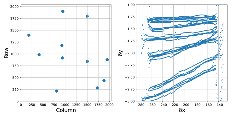
Figure 20: NGDEEP-NISSNIRISS Trace measurements using PID 01089 observations using the GRISM R crossed with the F200W imaging filter. The shape of traces were measured across the entire detector (Left Panel) and variation in the geometry of the spectral traces are readily visible in the Right Panel.

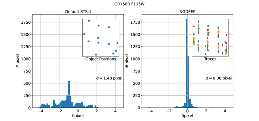
Figure 21: Comparison of the official NIRISS calibration and the NGDEEP-NISS calibration we adopted in this work when using the GR150C grism with the F115W filter. The left panel shows the histogram of the difference between measured and predicted location of the +1,+2,+3,-1 spectral orders. The inset of the Left Panel shows where calibration sources were located within the field of view of the instrument. The Right Panel shows the same histogram but computed using our NGDEEP-NISS calibration. The inset of the Right Panel shows where the +1,+2,+3,-1 order traces were located on the detector. .

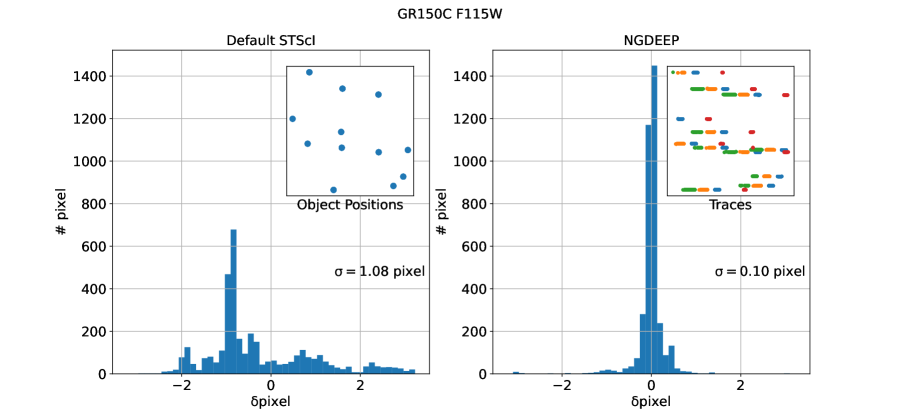
Figure 22: Same as Figure 21 but for the GR150R grism with the F115W filter.

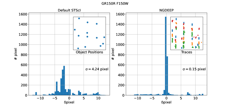
Figure 23: Same as Figure 21 but for the GR150R grism with the F150W filter.

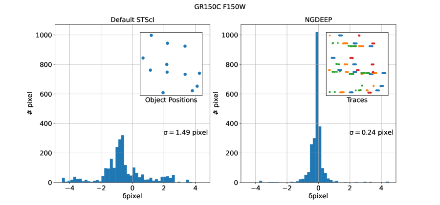
Figure 24: Same as Figure 21 but for the GR150C grism with the F150W filter.

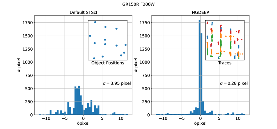
Figure 25: Same as Figure 21 but for the GR150R grism with the F200W filter.

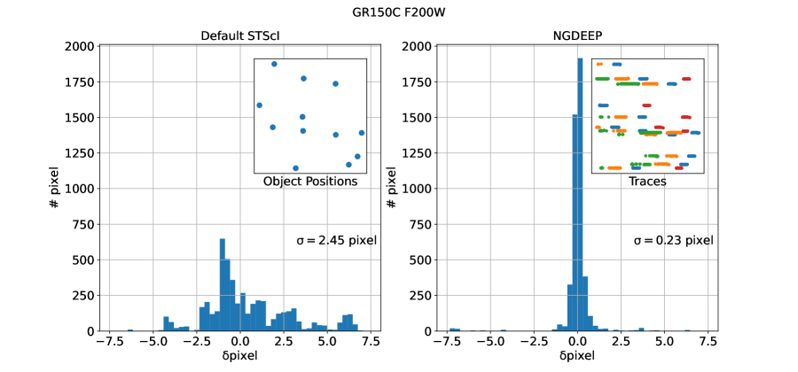
Figure 26: Same as Figure 21 but for the GR150C grism with the F200W filter.

Table 8: NGDEEP-NISS Calibration of Trace Geometry Residuals

GRISM	Filter	Default	NGDEEP-NISS
		${\rm Pixel}$	${\rm Pixel}$
GR150R	F115W	1.40	0.08
GR150R	F150W	4.08	0.15
GR150R	F200W	3.15	0.28
GR150C	F115W	0.90	0.10
GR150C	F150W	1.49	0.24
GR150C	F200W	3.15	0.28

B.2 Wavelength Calibration

NIRISS observed a wavelength calibrator (LMC PN58) at 9 positions across the detector, covering the a large part of the field of view. We extracted the NIRISS spectra of the target and proceeded to measure the location of the emission line along the spectral traces. A global field dependent solution can be determined by comparing the the observed positions along the traces to the fiducial wavelengths of the emission lines. As the NIRISS spectra have a limited wavelength range, we fit a single wavelength solution across the three cross filters we used, covering the weavelength range of $1<\mu m<2.2$. The fiducial wavelengths of the lines were obtained using NIRSPEC MOS observations of the target. We fit a 1st order polynomial with a 2nd order field dependence as this type of polynomial allowed us to derive solutions that reduced the residuals of the fit to a small fraction of a pixel, typically better than $20\AA$ or half of a pixel. This in contrast to the default calibration products which, even when extracting these spectra using the improved trace calibration described in the previous section, showed residuals getting progressively worse a the longer wavelengths on the order of several pixels/resolution elements or more ($\approx 20--120\AA$). Figures 27 and 28 show the differences between expected and predicted wavelengths along the traces of the R and G grisms. In summary, the NGDEEP-NISS wavelength calibration of the NIRISS grisms is typically within $\approx 10\AA$ which is approximately a quarter of a resolution element and therefore on a similar scale as the trace calibration described in the previous section. There is a significant amount of field dependence to the wavelength calibration as shown by the large spread of errors when using the default NIRISS WFSS calibration.

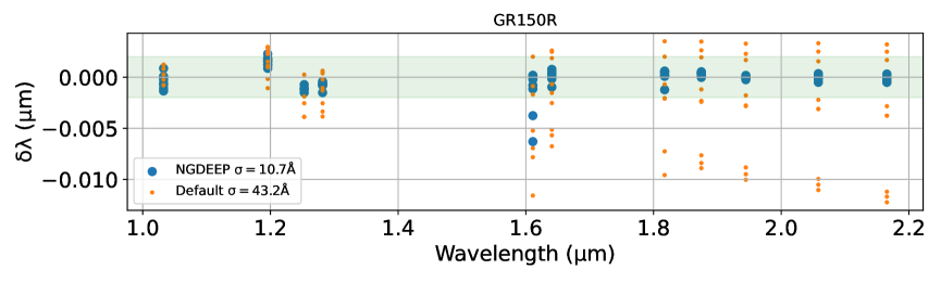
Figure 27: Difference in computed emission line wavelengths in observations of PN58 using the NGDEEP-NISS wavelength solution (blue) and the default available calibration (orange) when using the GR150R grism.

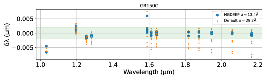
Figure 28: Same as Figure 27 but for the GR150C grism

References

- Ashton & Talbot (2021) Ashton, G., & Talbot, C. 2021, MNRAS, 507, 2037
- Atek et al. (2010) Atek, H., Malkan, M., McCarthy, P., et al. 2010, ApJ, 723, 104
- Bagley et al. (2023) Bagley, M. B., Pirzkal, N., Finkelstein, S. L., et al. 2023, arXiv e-prints, arXiv:2302.05466
- Baker & Menzel (1938a) Baker, J. G., & Menzel, D. H. 1938a, ApJ, 88, 52
- Baker & Menzel (1938b) —. 1938b, ApJ, 88, 52
- Baldwin et al. (1981) Baldwin, J. A., Phillips, M. M., & Terlevich, R. 1981, Publications of the Astronomical Society of the Pacific, 93, 5
- Beckwith et al. (2006) Beckwith, S. V. W., Stiavelli, M., Koekemoer, A. M., et al. 2006, AJ, 132, 1729
- Bertin & Arnouts (1996) Bertin, E., & Arnouts, S. 1996, A&AS, 117, 393
- Boquien et al. (2019) Boquien, M., Burgarella, D., Roehlly, Y., et al. 2019, A&A, 622, A103
- Brammer et al. (2014) Brammer, G., Pirzkal, N., McCullough, P., & MacKenty, J. 2014, Time-varying Excess Earth-glow Backgrounds in the WFC3/IR Channel, Instrument Science Report WFC3 2014-03, 14 pages
- Brammer et al. (2012) Brammer, G. B., van Dokkum, P. G., Franx, M., et al. 2012, ApJS, 200, 13
- Burgarella et al. (2005) Burgarella, D., Buat, V., & Iglesias-Páramo, J. 2005, MNRAS, 360, 1413
- Charlot & Fall (2000) Charlot, S., & Fall, S. M. 2000, ApJ, 539, 718
- Conroy et al. (2009) Conroy, C., Gunn, J. E., & White, M. 2009, ApJ, 699, 486
- Conroy et al. (2010) Conroy, C., White, M., & Gunn, J. E. 2010, ApJ, 708, 58
- Domínguez et al. (2013) Domínguez, A., Siana, B., Henry, A. L., et al. 2013, ApJ, 763, 145
- Doyon et al. (2023) Doyon, R., Willott, C. J., Hutchings, J. B., et al. 2023, PASP, 135, 098001
- Faisst et al. (2018) Faisst, A. L., Masters, D., Wang, Y., et al. 2018, ApJ, 855, 132
- Ferland (1999) Ferland, G. J. 1999, PASP, 111, 1524
- Gardner et al. (2023) Gardner, J. P., Mather, J. C., Abbott, R., et al. 2023, PASP, 135, 068001
- Grogin et al. (2011) Grogin, N. A., Kocevski, D. D., Faber, S. M., et al. 2011, ApJS, 197, 35
- Groves et al. (2012) Groves, B., Brinchmann, J., & Walcher, C. J. 2012, MNRAS, 419, 1402
- Horne (1986) Horne, K. 1986, PASP, 98, 609
- Johnson et al. (2021) Johnson, B. D., Leja, J., Conroy, C., & Speagle, J. S. 2021, ApJS, 254, 22
- Juneau et al. (2011) Juneau, S., Dickinson, M., Alexander, D. M., & Salim, S. 2011, ApJ, 736, 104
- Juneau et al. (2014) Juneau, S., Bournaud, F., Charlot, S., et al. 2014, ApJ, 788, 88
- Kennicutt & Evans (2012) Kennicutt, R. C., & Evans, N. J. 2012, ARA&A, 50, 531
- Kewley et al. (2013) Kewley, L. J., Maier, C., Yabe, K., et al. 2013, ApJ, 774, L10
- Koekemoer et al. (2011) Koekemoer, A. M., Faber, S. M., Ferguson, H. C., et al. 2011, ApJS, 197, 36
- Leung et al. (2023) Leung, G. C. K., Bagley, M. B., Finkelstein, S. L., et al. 2023, ApJ, 954, L46
- Luo et al. (2017) Luo, B., Brandt, W. N., Xue, Y. Q., et al. 2017, ApJS, 228, 2
- Luridiana et al. (2009) Luridiana, V., Simón-Díaz, S., Cerviño, M., et al. 2009, ApJ, 691, 1712
- Matharu et al. (2023) Matharu, J., Muzzin, A., Sarrouh, G. T. E., et al. 2023, ApJ, 949, L11
- Miller & Mathews (1972) Miller, J. S., & Mathews, W. G. 1972, ApJ, 172, 593
- Momcheva et al. (2016) Momcheva, I. G., Brammer, G. B., van Dokkum, P. G., et al. 2016, ApJS, 225, 27
- Noll et al. (2009) Noll, S., Burgarella, D., Giovannoli, E., et al. 2009, A&A, 507, 1793
- Oke & Gunn (1983) Oke, J. B., & Gunn, J. E. 1983, ApJ, 266, 713
- Osterbrock (1989) Osterbrock, D. E. 1989, Astrophysics of gaseous nebulae and active galactic nuclei
- Pagel & Edmunds (1981) Pagel, B. E. J., & Edmunds, M. G. 1981, ARA&A, 19, 77
- Pagel et al. (1979) Pagel, B. E. J., Edmunds, M. G., Blackwell, D. E., Chun, M. S., & Smith, G. 1979, MNRAS, 189, 95
- Papovich et al. (2022) Papovich, C., Simons, R. C., Estrada-Carpenter, V., et al. 2022, ApJ, 937, 22
- Pirzkal et al. (2017a) Pirzkal, N., Hilbert, B., & Rothberg, B. 2017a, Trace and Wavelength Calibrations of the UVIS G280 +1/-1 Grism Orders, Instrument Science Report WFC3 2017-20, 15 pages
- Pirzkal & Ryan (2017) Pirzkal, N., & Ryan, R. 2017, A more generalized coordinate transformation approach for grisms, Instrument Science Report WFC3 2017-01 (v.1), 9 pages
- Pirzkal & Ryan (2020) —. 2020, The Dispersed infrared background in WFC3 G102 and G141 observations, Instrument Science Report WFC3 2020-4, 32 pages
- Pirzkal et al. (2016) Pirzkal, N., Ryan, R., & Brammer, G. 2016, Trace and Wavelength Calibrations of the WFC3 G102 and G141 IR Grisms, Instrument Science Report WFC3 2016-15, 25 pages
- Pirzkal et al. (2004) Pirzkal, N., Xu, C., Malhotra, S., et al. 2004, ApJS, 154, 501
- Pirzkal et al. (2009) Pirzkal, N., Burgasser, A. J., Malhotra, S., et al. 2009, ApJ, 695, 1591
- Pirzkal et al. (2017b) Pirzkal, N., Malhotra, S., Ryan, R. E., et al. 2017b, ApJ, 846, 84
- Pirzkal et al. (2018) Pirzkal, N., Rothberg, B., Ryan, R. E., et al. 2018, ApJ, 868, 61
- Planck Collaboration et al. (2014) Planck Collaboration, Ade, P. A. R., Aghanim, N., et al. 2014, A&A, 571, A30
- Salim & Narayanan (2020) Salim, S., & Narayanan, D. 2020, ARA&A, 58, 529
- Scarlata (2023) Scarlata, C. 2023, Private Communication
- Shapley et al. (2022) Shapley, A. E., Sanders, R. L., Salim, S., et al. 2022, ApJ, 926, 145
- Simons et al. (2023) Simons, R. C., Papovich, C., Momcheva, I. G., et al. 2023, ApJS, 266, 13
- Speagle (2020) Speagle, J. S. 2020, MNRAS, 493, 3132
- Struve & Schwede (1931) Struve, O., & Schwede, H. F. 1931, Physical Review, 38, 1195
- Wang et al. (2009) Wang, J.-G., Dong, X.-B., Wang, T.-G., et al. 2009, ApJ, 707, 1334
- Whitaker et al. (2012) Whitaker, K. E., van Dokkum, P. G., Brammer, G., & Franx, M. 2012, ApJ, 754, L29
- Witt & Gordon (2000) Witt, A. N., & Gordon, K. D. 2000, ApJ, 528, 799