Scalable and hyper-parameter-free non-parametric covariate shift adaptation with conditional sampling

Abstract

Many existing covariate shift adaptation methods estimate sample weights to be used in the risk estimation in order to mitigate the gap between the source and the target distribution. However, non-parametrically estimating the optimal weights typically involves computationally expensive hyper-parameter tuning that is crucial to the final performance. In this paper, we propose a new non-parametric approach to covariate shift adaptation which avoids estimating weights and has no hyper-parameter to be tuned. Our basic idea is to label unlabeled target data according to the $k$-nearest neighbors in the source dataset. Our analysis indicates that setting $k=1$ is an optimal choice. Thanks to this property, there is no need to tune any hyper-parameters, unlike other non-parametric methods. Moreover, our method achieves a running time quasi-linear in the sample size with a theoretical guarantee, for the first time in the literature to the best of our knowledge. Our results include sharp rates of convergence for estimating the joint probability distribution of the target data. In particular, the variance of our estimators has the same rate of convergence as for standard parametric estimation despite their non-parametric nature. Our numerical experiments show that proposed method brings drastic reduction in the running time with accuracy comparable to that of the state-of-the-art methods.

1 Introduction

Traditional machine learning methods assume that the source data distribution $P$ and the target data distribution $Q$ are identical. However, this assumption can be violated in practice when there is a distribution shift (Chen et al., 2022) between them. Various types of shift have been studied in the literature, and one of the most common scenarios is covariate shift (Shimodaira, 2000) in which there is a shift in the input distribution: $P_{X}\neq Q_{X}$ while the conditional distribution of the output variable given the input variable is the same: $P_{Y\>|\>X}=Q_{Y\>|\>X}$, where $X$ is the input and $Y$ is the output variable. The goal of covariate shift adaptation is to adapt a supervised learning algorithm to the target distribution using labeled source data and unlabeled target data.

A standard approach to covariate shift is weighting source examples (Shimodaira, 2000). Many studies focused on improving the weights (Huang et al., 2006; Gretton et al., 2008; Yamada et al., 2013; Kanamori et al., 2009; Sugiyama et al., 2007, 2008; Aminian et al., 2022). We refer the reader to Section 5 for more details of related work. Since we rarely know the model for how the input distributions can be shifted a priori, non-parametric methods are particularly useful for covariate shift adaptation. Some of the existing methods allow one to use non-parametric models through kernels. However, such kernel-based methods take at least quadratic times in computing kernel matrices. Some methods further need to solve linear systems and take cubic times in the sample size unless one resorts to approximations (Williams and Seeger, 2000; Le et al., 2013). Moreover, their performance is often sensitive to the choice of hyper-parameters of the kernel. Typically, one performs a grid search $K$-fold cross-validation for selecting the hyper-parameters, which amplifies the running time by roughly $K\lvert\Gamma\rvert$, where $\Gamma$ is the set of candidates for the hyper-parameters. Moreover, the criterion for the hyper-parameter selection is not obvious either because we do not have access to the labels for the target data. One can use weighted validation scores using the labeled source data with importance sampling, but it is not straightforward to choose what weights to be used for the cross-validation when we are choosing weights.

In this paper, we propose a non-parametric covariate shift adaptation method that is scalable and has no hyper-parameter. Our idea is to generate synthetic labels for unlabeled target data using a non-parametric conditional sampler constructed from source data. Under the assumption of covariate shift, the target data attached with the generated labels behave like labeled target data. This sampling technique allows any supervised learning method to be applied simply to the generated data to produce a model already adapted to the target distribution.

We can use various sampling methods for the synthetic labeling part. In particular, we show that a $k$-nearest neighbor ($k$-NN) method achieves an excellent theoretical estimation performance, and, more importantly, our error bounds suggest that $k=1$ is the most favorable. This fact allows us to simply set $k=1$ and circumvent the cumbersome hyper-parameter tuning while providing computational efficiency at the same time. This is in contrast to the application of $k$-NN to standard density estimation, classification, or regression problems, in which we typically need to let $k$ grow in a polynomial rate in the sample size in order to achieve a good balance in the bias-variance trade-off. This analysis of ours leads to a non-parametric yet computationally efficient method: our $1$-NN-based algorithm takes only a quasi-linear time $\mathcal{O}((n+m)\log n)$ on average using the optimized $k$-d tree (Bentley, 1975; Friedman et al., 1977), where $n$ and $m$ are the source and the target sample size, respectively. We confirm the computational efficiency of the proposed method through experiments.

In summary, the key contributions of this paper are the following. (i) Our method is non-parametric. It does not introduce a model in covariate shift adaptation so that it will have a minimum impact on the model trained for the downstream task. (ii) Our method is fast. Adaptation only takes a quasi-linear time. (iii) There is no hyper-parameter to be tuned. (iv) The proposed method only incurs an error of order $\mathcal{O}_{p}\left({(k/n)^{1/d}+1/\sqrt{n}+1/\sqrt{m}}\right)$, where $d$ is the data dimentionality, for which we provide a non-asymptotic analysis.

2 Problem setup

In Section 1, we briefly introduced the setup of covariate shift adaptation that we consider in this paper. In this section, we will define the problem more formally.

Let $\mathcal{X}$ and $\mathcal{Y}$ be measurable spaces. Let $P\equiv P_{X,Y}$ and $Q\equiv Q_{X,Y}$ be probability distributions defined on $\mathcal{X}\times\mathcal{Y}$. Throughout the paper, we assume that $P$ and $Q$ admit the decomposition

$$P=P_{Y\>|\>X}P_{X}\quad\text{and}\quad Q=Q_{Y\>|\>X}Q_{X},$$

where $P_{Y\>|\>X=x}$ and $Q_{Y\>|\>X=x}$ are probability distributions defined on $\mathcal{Y}$ for each $x\in\mathcal{X}$. Here, $P_{X}$ and $Q_{X}$ are the marginal distributions of $X$ when $(X,Y)$ is distributed with $P$ and $Q$, respectively. We shall simply call $P_{Y\>|\>X}$ (or $Q_{Y\>|\>X}$) the conditional distribution of $Y$ given $X$.

Definition 1 (Source sample, source distribution).

For each integer $n\geq 1$, let $(X_{i},Y_{i})_{i=1}^{n}$ be a collection of independent identically distributed random variables with $P$. We refer to $(X_{i},Y_{i})_{i=1}^{n}$ as a (labeled) source sample and $P$ as a source distribution.

Definition 2 (Target sample, target distribution).

For each integer $m\geq 1$, let $(X^{*}_{i})_{i=1}^{m}$ be a collection of independent identically distributed random variables with $Q$. We refer to $(X^{*}_{i})_{i=1}^{m}$ as an (unlabeled) target sample and $Q$ as a target distribution.

Definition 3 (Covariate shift).

Covariate shift is a situation in which the source and the target distribution have different marginal distributions for $X$ while sharing a common conditional distribution:

1. $P_{Y\>|\>X}=Q_{Y\>|\>X}$, $P_{X}$- and $Q_{X}$-a.s., but $P_{X}\neq Q_{X}$.

This paper focuses on the following simple but versatile estimation problem under covariate shift.

Definition 4 (Mean estimation under covariate shift).

For each pair of integers $n\geq 1$, $m\geq 1$, and a known integrable function $h\colon\mathcal{X}\times\mathcal{Y}\to\mathbb{R}$, the goal of mean estimation under covariate shift is to estimate the mean of $h$ under the target distribution, $Q(h)\equiv\int h(x,y)Q(dx,dy)$, given access to the source sample $(X_{i},Y_{i})_{i=1}^{n}\sim P$ and the target sample $(X^{*}_{i})_{i=1}^{m}\sim Q_{X}$ under Assumption (C1).

For instance, when $h(x,y)=\ell(f(x),y)$ for some loss function and hypothesis function $f$, estimation of $Q(h)$ becomes risk estimation, which is the central subtask in empirical risk minimization.

3 Proposed method

The basic idea of our proposed method is to use the source sample for learning to label the target data. Specifically, using the source sample $(X_{i},Y_{i})_{i=1}^{n}$, we construct a stochastic labeling function $\hat{\texttt{S}}$ that inputs any target data point $X^{*}_{i}$ and outputs a random label $Y^{*}_{n,i}\in\mathcal{Y}$. (The subscript $n$ of $Y^{*}_{n,i}$ is for explicitly denoting the dependence on the source sample.) Once we succeed in generating labels for target data that behave like true target labels, we will be able to perform any supervised learning method directly on the target sample for the downstream task. For our mean estimation problem, we can simply average the output $h$ evaluated at the target data with the generated labels.

When do the generated labels behave like the true target labels? Let $\hat{P}_{Y\>|\>X^{*}_{i}}$ denote the probability distribution of an output $Y^{*}_{n,i}$ of $\hat{\texttt{S}}$ for input $X^{*}_{i}$. We wish to obtain $\hat{\texttt{S}}$ such that the probability distribution $\hat{Q}\equiv\hat{P}_{Y\>|\>X}Q_{X}$ of $(X^{*}_{i},Y^{*}_{n,i})$ will be a good estimate of $Q=Q_{Y\>|\>X}Q_{X}$. For this, we want $\hat{P}_{Y\>|\>X^{*}_{i}}$ to be a good estimate of $P_{Y\>|\>X^{*}_{i}}$. In fact, if $\hat{P}_{Y\>|\>X^{*}_{i}}=P_{Y\>|\>X^{*}_{i}}$, the generated sample $(X^{*}_{i},Y^{*}_{n,i})$ will follow the target distribution $Q\equiv Q_{Y\>|\>X}Q_{X}=P_{Y\>|\>X}Q_{X}$ under Assumption (C1). In this sense, our task boils down to designing a good conditional sampler for $\hat{\texttt{S}}$. Algorithm 1 describes an outline of this general framework.

Algorithm 1 Conditional-sampling Covariate-shift Adaptation (CSA)

Input: conditional sampler $\hat{\texttt{S}}$ and target sample $(X^{*}_{j})_{j=1}^{m}$.

$Y^{*}_{n,j}\leftarrow\hat{\texttt{S}}(X_{j}^{*})$ for each $j\in\{1,\dots,m\}$. // Generate a label conditioned on $X_{j}^{*}$.

return $m^{-1}\sum_{j=1}^{m}h(X^{*}_{j},Y^{*}_{n,j})$.

In this paper, we propose using a non-parametric conditional sampler $\hat{\texttt{S}}$ based on the $k$-Nearest Neighbor ($k$-NN) method in CSA, which randomly outputs one of the $k$-nearest neighbors of input $X^{*}_{j}$ in the source sample $(X_{i},Y_{i})_{i=1}^{n}$ (Algorithm 2). We refer to this $k$-NN-based CSA as $k$-NN-CSA.

Algorithm 2 $k$-Nearest Neighbor Conditional Sampler

Input: Source sample $(X_{i},Y_{i})_{i=1}^{n}$ and target input $X^{*}_{j}$.

$(i_{1},\dots,i_{k})\leftarrow\text{the indices of the $k$-nearest neighbors of $X^{*}_{j}$ in the source instances $(X_{i})_{i=1}^{n}$}$.

Pick $i^{*}\in\{i_{1},\dots,i_{k}\}$ uniformly at random.

return $Y^{*}_{n,j}:=Y^{*}_{i^{*}}$.

Computing time

Recent advances for nearest neighbor search rely on tree-search to reduce the computing time. The seminal paper by Bentley (1975) introduces the $k$-d tree method. Building such a tree requires $\mathcal{O}(n\log n)$ and once the tree is available, search for the nearest neighbor of a given point can be done in $\mathcal{O}(\log n)$ time (Friedman et al., 1977). As a consequence, the time complexity of $k$-NN-CSA is $\mathcal{O}(n\log n+km\log n)$.

4 Theoretical analysis

The theory behind our approach is now presented in a didactic way by first introducing a key decomposition and then studying separately each of the terms involved: the sampling error and the $k$-NN estimation error. We will see that $k$-NN-based CSA ($k$-NN-CSA for short) with $k=1$ admits excellent theoretical performance.

4.1 A key decomposition

For the analysis of $k$-NN-CSA, recall that $\hat{Q}=\hat{P}_{Y|X}Q_{X}$ is an estimate of the target distribution $Q=P_{Y|X}Q_{X}$ that depends on the source sample $(X_{i},Y_{i})_{i=1}^{n}$ whose probability distribution is $P$. We introduce the bootstrap sample as a collection of random variable generated according to $\hat{Q}$.

Definition 5 (Bootstrap sample).

For each $m\geq 1$ and $n\geq 1$, let $(X_{i}^{*},Y_{n,i}^{*})_{1\leq i\leq m}$ be a collection of random variables identically distributed with $\hat{Q}$ and conditionally independent given $(X_{i},Y_{i})_{i=1}^{n}$.

Let $h:\mathcal{X}\times\mathcal{Y}\to\mathbb{R}$ be a measurable function. The object of interest is the following quantity

$$\hat{Q}^{*}(h)=m^{-1}\sum_{i=1}^{m}h(X_{i}^{*},Y_{n,i}^{*}),$$

which is the CSA estimate of $Q(h)=\int h(x,y)Q(dx,dy)$ as introduced in Algorithm 1. The following decomposition is crucial in our analysis:

$$(\hat{Q}^{*}-Q)(h)=(\hat{Q}^{*}-\hat{Q})(h)+(\hat{Q}-Q)(h).$$ (1)

The first term is a sampling error which can easily be small as soon as $m$ is large. The second term represents the accuracy that we should obtain when estimating the target measure $Q$. When using the $k$-nearest neighbor algorithm to obtain $\hat{Q}$, we show that this term is of order $(k/n)^{1/d}+1/\sqrt{n}$, which differs from standard non-parametric convergence rate in $(k/n)^{1/d}+1/\sqrt{k}$.

4.2 Sampling Error

We are interested in the sampling error, i.e., $(\hat{Q}^{*}-\hat{Q})(h)$, and the aim is to show that it is of order $1/\sqrt{m}$. The analysis relies on martingale tools. Define $\mathcal{F}_{n}=\sigma((X_{1},Y_{1}),\ldots,(X_{n},Y_{n}))$. For each $1\leq i\leq m$, we have

$$\mathbb{E}[h(X_{i}^{*},Y_{n,i}^{*})\>|\>\mathcal{F}_{n}]=\hat{Q}(h).$$

This property implies that $\sum_{i=1}^{m}\{h(X_{i}^{*},Y_{n,i}^{*})-\int h(x,y)\,\hat{Q}(dx,dy)\}$ is a martingale and therefore can be analyzed using the Lindeberg-CLT conditionally on the initial sample hence fixing the distribution $\hat{Q}$. The next property is reminiscent of certain results about the bootstrap method where sampling is done with the basic empirical measure, see e.g., Van der Vaart (2000). We need this type of results without specifying the measure $\hat{Q}$ so that we can incorporate a variety of sampling schemes such as $\hat{Q}=\hat{P}_{Y\>|\>X}Q_{X}$. The proof is given in the supplementary material.

Proposition 1.

Suppose that $\hat{Q}$ satisfies the following strong law of large number: for each $h$ such that $Q(h)<\infty$, we have $\lim_{n}\hat{Q}(h)=Q(h)$ almost surely. Then, if $m:=m_{n}\to\infty$ as $n\to\infty$, we have the following central limit theorem: for each function such that $Q(h^{2})<\infty$, we have, conditionally to $\mathcal{F}_{n}$, almost surely,

$$\sqrt{m}\{\hat{Q}^{*}(h)-\hat{Q}(h)\}\leadsto\mathcal{N}(0,V)\qquad\text{as }n\to\infty,$$

where $V=\lim_{n}\{\hat{Q}(h^{2})-\hat{Q}(h)^{2}\}$.

As a corollary of the previous results, we can already deduce that if $m$ goes to $\infty$ and $\hat{Q}$ satisfies a strong law of large numbers, then $\hat{Q}^{*}(h)$ converges to $Q(h)$ provided that $Q(h^{2})$ exists. This is a general consistency result that justifies the use of any resampling distribution $\hat{Q}$ that converges to $Q$. In practical situations, it is useful to know a finite-sample bound on the error. This is the purpose of the next proposition, in which we give a non-asymptotic control of the sampling error. A proof is given in the supplementary material.

Proposition 2.

Suppose that $h$ is bounded by a constant $U_{h}>0$. Let $\delta\in(0,1)$. Then with probability greater than $1-\delta$,

$$\left|\hat{Q}^{*}(h)-\hat{Q}(h)\right|\leq\frac{U_{h}}{m}\log(2/\delta)+\sqrt{2\frac{\hat{v}_{n}}{m}\log(2/\delta)}.$$

where $\hat{v}_{n}=\hat{Q}(h^{2})-(\hat{Q}h)^{2}$.

4.3 Nearest neighbor estimate

Our aim in this section is to obtain a bound on $\hat{Q}(h)-Q(h)$ (the second term in our decomposition (1)) when $\hat{P}_{Y|X}$ is the $k$-nearest neighbor measure.

Let $x\in\mathbb{R}^{d}$ and $\lVert\cdot\rVert$ be the Euclidean norm on $\mathbb{R}^{d}$. Denote the closed ball of radius $\tau\geq 0$ around $x$ by $B(x,\tau):=\{z\in\mathbb{R}^{d}\mid\lVert x-z\rVert\leq\tau\}$. For $n\geq 1$ and $k\in\{1,\;\ldots,\;n\}$, the $k$-nearest neighbor ($k$-NN for short) radius at $x$ is denoted by $\hat{\tau}_{n,k,x}$ and defined as the smallest radius $\tau\geq 0$ such that the ball $B(x,\tau)$ contains at least $k$ points from the collection $\{X_{1},\ldots,X_{n}\}$. That is,

$$\hat{\tau}_{n,k,x}:=\inf\left\{\tau\geq 0\,:\,\sum_{i=1}^{n}1_{B(x,\tau)}(X_{i})\geq k\right\},$$

where $1_{A}(x)$ is $1$ if $x\in A$ and $0$ elsewhere. The $k$-NN estimate of $P_{Y\>|\>X}(dy\>|\>x)$ is given by

$$\hat{P}_{Y\>|\>X}(dy\>|\>x)=k^{-1}\sum_{i=1}^{n}1_{\lVert X_{i}-x\rVert\leq\hat{\tau}_{n,k,x}}\delta_{Y_{i}}(dy),$$

where $\delta_{y}(\cdot)$ is the Dirac measure at $y\in\mathcal{Y}$ defined by $\delta_{y}(A)=1_{A}(y)$ for any measurable set $A\subseteq\mathcal{Y}$. Consequently, the $k$-NN estimate of the integral $\int h(y,x)P_{Y\>|\>X}(dy\>|\>x)$ is then defined as

$$\int h(y,x)\hat{P}_{Y\>|\>X}(dy\>|\>x)=k^{-1}\sum_{i=1}^{n}1_{\|X_{i}-x\|\leq\hat{\tau}_{n,k,x}}h(Y_{i},x).$$

To obtain some guarantee on the behavior of the nearest neighbors estimate, we consider the case in which covariates $X$ admit a density with respect to the Lebesgue measure. We will need in addition that the support $S_{X}$ is well shaped and that the density is lower bounded. These are standard regularity conditions to obtain some upper bound on the $k$-NN radius.

1. The random variable $X$ admits a density $p_{X}$ with compact support $S_{X}\subset\mathbb{R}^{d}$.

2. There is $c>0$ and $T>0$ such that

   $$\lambda(S_{X}\cap B(x,\tau))\geq c\lambda(B(x,\tau)),\qquad\forall\tau\in(0,T],\,\forall x\in S_{X},$$

   where $\lambda$ is the Lebesgue measure.

3. There is $0<b_{X}\leq U_{X}<+\infty$ such that $b_{X}\leq p_{X}(x)\leq U_{X}$, for all $x\in S_{X}$.

To obtain our main result, on the estimation property of the $k$-NN measure, we need some assumptions on the target measure $Q_{X}$.

1. The probability measure $Q_{X}$ admits a bounded density $q_{X}$ with support $S_{X}$. We will take $U_{X}$ large enough such that it will also be an upper bound of $q_{X}$.

Two additional assumptions, different from the one before about $X$, will be needed to deal with the function $h$ and the probability distribution of $(Y,X)$.

1. For any $x$ in $S_{X}$,

   $$\lvert\mathbb{E}[h(Y,x)\>|\>X=x]-\mathbb{E}[h(Y,x)\>|\>X=x+u]\rvert\leq g_{h}(x)\lVert u\rVert$$

   with $\int g_{h}(x)Q_{X}(dx)<\infty$.

2. There exists $\sigma_{h}^{2}>0$ such that $\sup_{x\in S_{X}}\operatorname{Var}(h(Y,x)\>|\>X)\leq\sigma_{h}^{2}\text{ a.s.}$, where $\operatorname{Var}(h(Y,x)\>|\>X)$ is the conditional variance of $h(Y,x)$ given $X$.

In what follows, we give a control of the RMSE of $\hat{Q}h$. Let $\|X\|_{2}=\sqrt{\mathbb{E}\left(X^{2}\right)}$ and let $\Gamma(x):=\int_{0}^{\infty}u^{x-1}\exp(-u)du$ for $x>0$. Finally, we denote by $V_{d}:=\lambda(B(0,1))=\frac{\pi^{d/2}}{\Gamma(d/2-1)}$ the volume of the unit Euclidean ball in dimension $d$ for the Lebesque measure.

We give an upper-bound for the RMSE with explicit constants with respect to the dimension $d$. Additionally, we give a lower bound for the variance which has a standard parametric rate of convergence.

Proposition 3.

Suppose that (X1), (X2), (X3), (X4), (H1), and (H2) are fulfilled. We have

$$\hat{Q}h-Qh=S_{h}+B_{h}$$

where $B_{h}$ is a bias term (defined in the proof) that satisfies, for any $n\geq 1$,

$$\mathbb{E}|B_{h}|\leq 2^{\frac{2}{d+1}}\Gamma\left(\frac{1}{d}+1\right)(cb_{x}V_{d})^{-1/d}\int g_{h}(x)Q_{X}(dx)\cdot\frac{k^{1/d}}{n^{1/d}}.$$

and $S_{h}$ is a variance term (defined in the proof) that satisfies, for any $n\geq 3$ and any $k\leq n/2$,

$$C_{1}n^{-1}\leq\min_{1\leq k<n/2}\mathbb{E}\left[S_{h}^{2}\right]\leq\max_{1\leq k<(n+3)/4}\mathbb{E}\left[S_{h}^{2}\right]\leq C_{2}n^{-1},$$

where $C_{1}$ and $C_{2}$ (defined in the proof) depends on $d$, $Q_{X}$, $P_{X}$ but not on $k$ and $n$. (For the lower bound to be true the density of $Q_{X}$ is lower bounded by $b_{X}$ as for $P_{X}$ and it is assumed that the mapping $h$ does not depend on $x$, i.e. $h(y,x)=h(y)$.)

Notes.

(i) The two terms $B_{h}$ and $S_{h}$ correspond respectively to the bias term and the variance term. The upper bound obtained for the bias term is usual in $k$-NN regression analysis. However, the variance upper and lower bound are typical to our framework as they show that the variance behaves as in usual parametric estimation. Consequently, our rates of convergence are sharper than the optimal rate of convergence $n^{-\frac{1}{2+d}}$ for nonparametric estimation of Lipschitz functionals. This can be explained by the fact that several $k$-NN estimators are averaged to estimate $Qh$ which is a standard expectation and not a conditional expectation.

(ii) Since the rate of convergence of the variance term $S_{h}$ does not depend on $k$, $k$ might be chosen according to the upper bound on the bias term, which gives $k=1$. One can deduce the following convergence rates, depending on the dimension. For $d=1$, we get the rate $n^{-1/2}$. For $d=2$, both terms, $B_{h}$ and $S_{h}$, contributions coincide and we get the rate $n^{-1/2}$. For $d\geq 3$, the rate is $n^{-1/d}$.

We next give a non-asymptotic control of $\hat{Q}h-Qh$ when $h$ is a bounded function using Bernstein’s concentration inequality. This bound affords a complement with respect to the bound for the MSE. However, for technical reasons, it requires that $k$ grows at least logarithmically with respect to $n$. In our numerical experiments, we will also include the case $k=\log n$ for comparison.

Proposition 4.

Suppose that (X1), (X2), (X3), (X4), (H1), and (H2) are fulfilled. Suppose that there exists a constant $C>0$ such that $C\log n\leq k\leq n/2$ and that $h$ is bounded by $U_{h}$. Let $\delta\in(0,1/3)$. With probability greater than $1-3\delta$, we have

$$\left|\hat{Q}h-Qh\right|\leq L_{0}\left(\frac{k}{n}\right)^{1/d}+\frac{2L_{2}}{n}\log(2/\delta)+\sqrt{\frac{2L_{1}\sigma^{2}}{n}\log(2/\delta)},$$

where

$$L_{0}=\left(\frac{2}{cb_{x}V_{d}}\right)^{1/d}\int g_{h}(x)Q_{X}(dx),\quad L_{1}=\frac{4\sigma_{h}^{2}U_{X}^{2}}{b_{X}^{2}c^{2}},\quad L_{2}=\frac{4U_{h}U_{X}}{3b_{X}c}.$$

Notes.

(i) The proof needs a bound on $\sup_{x\in S_{X}}\hat{\tau}_{n,k,x}$ which is given in (Portier, 2021, Lemma 4). For this we need that $k$ grows logarithmically w.r.t. $n$ as stated in the assumptions.

(ii) The sum of the two last terms in the upper-bound, which corresponds to the variance of our estimator, is of order $1/\sqrt{n}$ and the conditional variance of $h$ appears as a multiplicative factor. Combining Proposition 2 and Proposition 4, we finally obtain that $\hat{Q}^{*}(h)-Q(h)$ is of order $1/\sqrt{m}+1/\sqrt{n}+(k/n)^{1/d}$ (up to log factors).

(iii) In Corollary 1 in the supplementary file, the upper bound given in Proposition 2 is refined using Proposition 4 that allows to (roughly speaking) replace the empirical variance by the true variance.

5 Related work

A standard approach to covariate shift problems is to use some re-weighting in order to “transfer” the source distribution with density $p_{X}$ to the target distribution with density $q_{X}$. This approach relies on the following type of estimates:

$$\hat{Q}_{w}(h)=n^{-1}\sum_{i=1}^{n}w(X_{i})h(X_{i},Y_{i}),$$

where ideally the function $w$ would take the form $q_{X}/p_{X}$. Such a choice has the nice property that the expected value $\mathbb{E}[w(X_{i})h(X_{i},Y_{i})]$ is equal to the targeted quantity $Q(h)$. This however cannot be directly computed as $p_{X}$ and $q_{X}$ are unknown in practice. There are actually different ways to estimate $w$, and our goal here is to distinguish between two leading approaches.

Plug-in

The plug-in approach is when the weights are computed using two estimates $\hat{p}_{X}$ and $\hat{q}_{X}$ in place of $p_{X}$ and $q_{X}$, respectively; i.e., simply use $\hat{w}=\hat{q}_{X}/\hat{p}_{X}$ instead $w$ in the above formula, see for instance (Shimodaira, 2000; Sugiyama et al., 2007, 2008). Note that the selection of hyper-parameters for $\hat{q}_{X}$ and $\hat{p}_{X}$ is needed and the $n$ evaluation $(\hat{q}_{X}(X_{i}),\hat{p}_{X}(X_{i}))$ might be heavy in terms of computing time.

For the sake of clarity, we focus on a specific instance of covariate shift problem in which the target probability density $q_{X}$ is known and ${\hat{p}}$ is the kernel density estimate (KDE), i.e., $\hat{p}_{X}^{KDE}(x)=(1/n)\sum_{i=1}^{n}K_{b}(x-X_{i})$, where $K_{b}$ typically is a Gaussian density with mean $0$ and variance $b^{2}$ (a hyper-parameter to be tuned). Note that such a situation does not involve any changes for our sampling procedure whereas it is clearly advantageous for the weighted approach for which one unknown, $q_{X}$, is now given. In this case, the analysis of $\hat{Q}_{w}(h)$ can be carried out using the decomposition $\hat{Q}_{\hat{w}}(h)-Q(h)=\hat{Q}_{\hat{w}}(h-Th)+\hat{Q}_{\hat{w}}(Th)-Q(h)$, with $Th(x)=\mathbb{E}[h(X,Y)|X=x]$. The first term above is a sum of centered random variable which (provided some conditions) satisfies the so-called Lindeberg condition so that the central limit theorem implies that $\sqrt{n}\hat{Q}_{\hat{w}}(h-Th)$ is asymptotically Gaussian. The second term above is more complicated and the analysis can be derived using results in Delyon and Portier (2016); Clémençon and Portier (2018). Those results assert (under some conditions) that $\hat{Q}_{\hat{w}}(Th)-Q(h)=O_{p}(nb^{d}+b)$ (in case $p_{X}$ is Lipschitz ). As a consequence, we obtain, optimizing over $b$, that $\hat{Q}_{\hat{w}}(h)-Q(h)=O_{p}(n^{-1/2}+n^{-1/(1+d)})$. This is easily compared to our bound, when $q_{X}$ is known, $n^{-1/2}+n^{-1/d}$, which is smaller than the one given before.

Direct weight estimation

Huang et al. (2006) proposed Kernel Mean Matching (KMM) for estimating the ratios of the probability density functions of the source and the target distribution. They used the estimated ratios for weighting the source sample. Gretton et al. (2008) further studied this method theoretically and empirically. Sugiyama et al. (2007, 2008) proposed a method that estimates the ratios as a function by minimizing the Kullback-Leibler divergence between the source density function multiplied by the ratio function and the target density function. The estimated function can predict ratios even outside of the source sample, which enables cross-validation for hyper-parameter tuning. Kanamori et al. (2009) proposed constrained and unconstrained least squares methods for estimating the ratio function called Least-Squares Importance Fitting (LSIF) and unconstrained LSIF (uLSIF). Yamada et al. (2013) developed its variant called Relative uLSIF (RuLISF), which replaces the denominator of the ratio with a convex mixture of the source and the target density functions to circumvent issues caused by near-zero denominators. Zhang et al. (2021) proposed a covariate shift adaptation method that directly minimizes an upper bound of the target risk in order to avoid estimation of weights. The method shows great empirical performance while it does not exactly minimize the target risk and hence the minimizer converges to a biased solution.

Other references

The idea of nonparametric sampling is a standard one in the field of texture synthesis. In particular, the choice of 1-NN resampling was often used as a fast method to generate new textures from a small sample. See Truquet (2011) for a literature review in this context. Our conditional sampling framework bears resemblance with traditional bootstrap sampling as there is random generation according to some estimated distribution. In contrast, the original bootstrap method is usually made up using draws from the standard empirical measure $(1/n)\sum_{i=1}^{n}\delta_{X_{i},Y_{i}}$. Here another distribution, $\hat{P}$, has been used to generate new samples. Moreover, our goal is totally different here. While the bootstrap technique was initially introduced for making inference, here the goal is to estimate an unknown quantity $Q(h)$ which appears in many machine learning tasks. Kpotufe and Martinet (2021) theoretically study covariate shift adaptation under the assumption that we have access to a labeled sample both from the source and the target distribution. Although they consider a $k$-nearest-neighbor-based method, it is essentially different from ours since they perform the $k$-NN method on the union of the source and the target sample. Lee et al. (2013) proposed pseudo-labeling unlabeled data in the context of semi-supervised learning. Wang (2023) uses the idea of pseudo-labeling in covariate shift adaptation. The author focuses on model selection in regression problems while we study the mean estimation that can be applied to a wider range of supervised learning problems.

6 Experiments

In this section, we present experiments using synthetic and real-world data. We test our proposed method with $k=1$ and $k=\log n$ referred to as $1$-NN-CSA and $\log n$-NN-CSA, respectively. We compare our method with the following non-parametric methods. KDE Ratio Weighting (KDER-W): the weighting method using the ratio of KDEs of $p_{X}$ and $q_{X}$ (see Section 5). KMM-W: the weighting method estimating $q_{X}/p_{X}$ using kernel mean matching. KLIEP-W: the weighting method estimating $q_{X}/p_{X}$ by minimizing the KL-divergence. RuLSIF-W: the weighting method using $q_{X}/(\alpha p_{X}+(1-\alpha)q_{X})$, where $\alpha\in[0,1]$ is a hyper-parameter. We use the default value $\alpha=0.1$. See Section 5 for brief explanations of those methods. For KMM-W, KLIEP-W, and RuLSIF-W, we used the implementations from Awesome Domain Adaptation Python Toolbox (ADAPT) (de Mathelin et al., 2021) and ran experiments on Google Colaboratory (https://colab.google). Our code and more details are in the supplementary material. Finally, we include the result for taking the average $\frac{1}{m}\sum_{i=1}^{m}h(X^{*}_{i},Y^{\circ}_{i})$ using a sample $(X^{*}_{i},Y^{\circ}_{i})_{i=1}^{m}\sim Q^{m}$ although $Y^{\circ}_{i}$ are not available in practical scenarios of our interest. We call this method OracleQ.

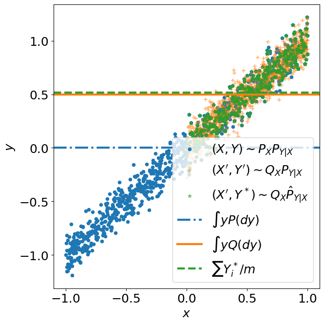
(a) Data

(b) Errors

(c) Times

Figure 2: Risk estimation experiment

Mean estimation using synthetic data We set $h$ as $h(x,y):=y$, $P_{X}$ as the uniform distribution over $[-1,1]$, $Q_{X}$ as that over $[0,1]$, and $P_{Y|X=x}$ as the normal distribution with mean $x$ and variance $0.1$. Figure 2(a) in Appendix A.8 shows an illustration of the setup. In this setup, we have $P(h)=\iint y\,P_{Y|X}(dy\>|\>x)P_{X}(dx)=0$ and $Q(h)=\iint y\,P_{Y|X}(dy\>|\>x)Q_{X}(dx)=0.5$. Note that estimation only using the source data from $P$ without covariate shift adaptation would fail to estimate $Q(h)=0.5$.

Figures 1(a)–1(b) shows the results. From Figure 1(a), we can see that $1$-NN-CSA outperforms the baseline method KDER-W and approaches OracleQ. The errors decrease roughly following power laws, where the slope of a line corresponds to the power of the convergence rate (steeper is better). We can see that $1$-NN-CSA seems to have the fastest convergence. Figure 1(b) shows the comparison in running times. $1$-NN-CSA and $\log n$-NN-CSA are much more scalable than the KDER-W.

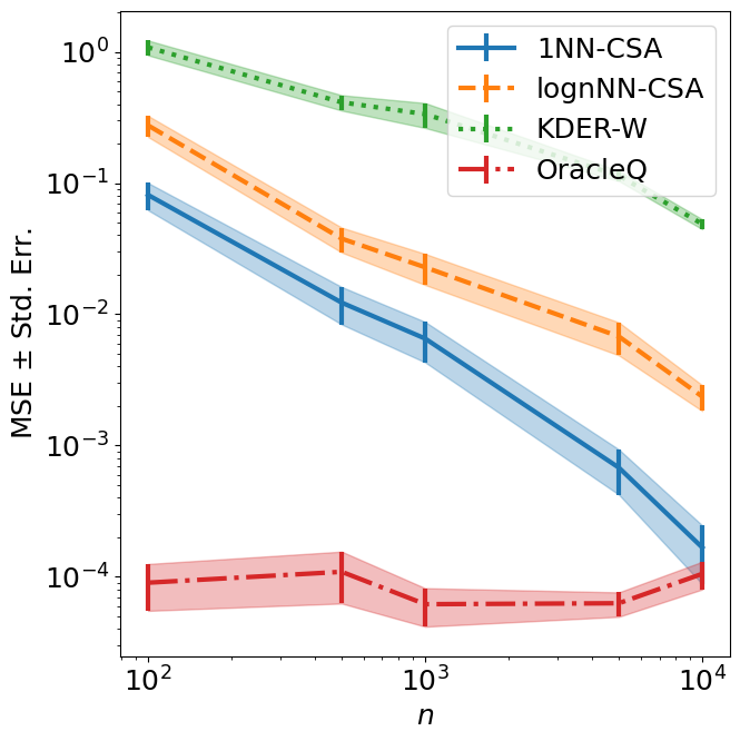
(a) Estimation errors

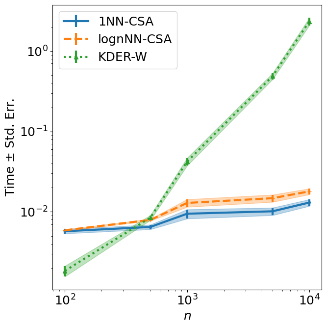
(b) Computation times

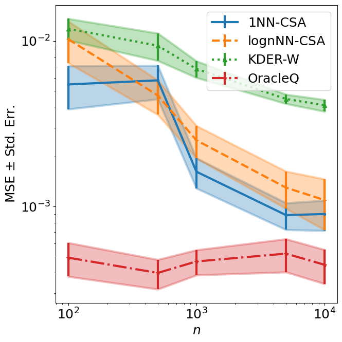
(c) Estimation errors.

(d) Computation times.

Figure 1: Results for the mean estimation (1(a)–1(b)) and risk estimation (1(c)–1(d)) experiments

Risk estimation experiment using synthetic data

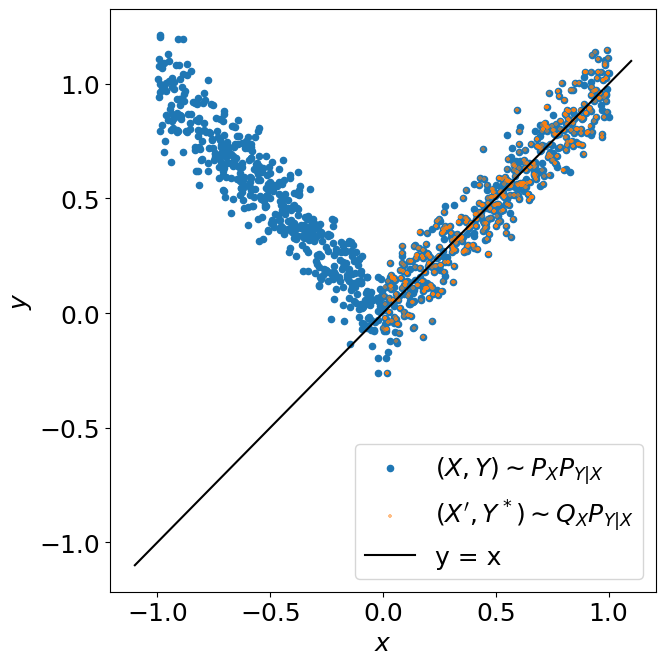
(a) Data

(b) Errors and sample size in logarithmic scale.

(c) Running times and sample size in logarithmic scale.

Figure 3: Risk estimation experiment

In this experiment, we compare the methods in the context of risk estimation of a fixed function $f_{0}$. We use the identify function $f_{0}\colon x\mapsto x$ and estimate the expected loss (i.e., risk) of $f_{0}(X)$ with the $\ell_{1}$ loss in predicting the output variable $Y$ when $(X,Y)$ follows $Q$. For this, we set $h$ as $h(x,y):=\lvert y-f_{0}(x)\rvert$, and the goal is to estimate the risk $Q(h)=\int\lvert y-f_{0}(x)\rvert Q(dx,dy)$. We use the uniform distribution over $[-1,1]$ for $P_{X}$ and that over $[0,1]$ for $Q_{X}$. We use the normal distribution with mean $\lvert x\rvert$ and variance $0.1$ for $P_{Y|X=x}$ for any $x\in\mathcal{X}:=[-1,1]$. See Figure 3(a) for an illustration of the setup. In this setup, the risks under $P_{X}$ and $Q_{X}$ are quite different because $f_{0}$ fits well in the support of $Q_{X}$ but not in that of $P_{X}$.

Figure 1(c) and Figure 1(d) show the results for the risk estimation experiment. The tendency is similar to the previous mean estimation experiment, but $1$-NN-CSA has a clearer advantage in computation time even over $\log n$-NN-CSA.

Linear regression and logistic regression experiments using benchmark datasets

We use regression benchmark datasets twonorm, diabetes, classification datasets ringnorm${}^{\ref{footnote:delve}}$, adult${}^{\ref{footnote:uci}}$, and breast_cancer${}^{\ref{footnote:uci}}$. We apply the ridge regression and the logistic regression, respectively. The evaluation metric is the coefficient of determination (denoted by $R^{2}$) for the regression tasks and the classification accuracy for classification tasks. We synthetically introduce covariate shift by subsampling test data. Refer to the supplementary material for more details.

Table 1: Coefficient of determination ($R^{2}$)/accuracy for regression/classification benchmark datasets. Larger is better for both evaluation metrics. We repeat the experiment using 50 different random sub-samples and calculate the average scores (and standard errors). The results comparable to the best in terms of Wilcoxon’s signed rank test with significance level $1\%$ are shown in bold.

	Regression ($R^{2}$)		Classification (accuracy)
	twonorm	diabetes	ringnorm	adult	breast_cancer
1NN-CSA	0.773 (0.002)	0.408 (0.009)	0.639 (0.017)	0.796 (0.012)	0.958 (0.002)
log-n-NN-CSA	0.773 (0.002)	0.408 (0.009)	0.639 (0.017)	0.796 (0.012)	0.957 (0.003)
KMM-W	0.741 (0.003)	0.456 (0.008)	0.710 (0.017)	0.789 (0.016)	0.960 (0.003)
RULSIF-W	0.741 (0.003)	0.456 (0.008)	0.729 (0.007)	0.837 (0.010)	0.963 (0.003)
KLIEP-W	0.741 (0.003)	0.456 (0.008)	0.710 (0.017)	0.789 (0.016)	0.960 (0.003)
KDE-R-W	0.521 (0.011)	0.404 (0.009)	0.585 (0.020)	0.797 (0.013)	0.956 (0.003)

Table 2: Total running times in seconds spent for the training including the hyper-parameter tuning (if any) for benchmark datasets. We repeat the experiment using 50 different random subsamples dataset and calculate the average running times (and standard errors). The results comparable to the best in terms of Wilcoxon’s signed rank test with significance level $1\%$ are shown in bold.

	twonorm	diabetes	ringnorm	adult	breast_cancer
1NN-CSA	0.002 (0.000)	0.001 (0.000)	0.003 (0.000)	0.118 (0.006)	0.001 (0.000)
log-n-NN-CSA	0.003 (0.000)	0.001 (0.000)	0.003 (0.000)	0.158 (0.006)	0.001 (0.000)
KMM-W	1.46 (0.05)	35.4 (0.5)	6.35 (1.29)	163 (5)	32.8 (0.3)
RULSIF-W	2.63 (0.15)	33.8 (0.6)	6.27 (0.27)	11.2 (0.4)	34.4 (0.6)
KLIEP-W	12.4 (0.4)	34.5 (0.5)	15.8 (0.6)	26.5 (1.1)	53.7 (0.5)
KDE-R-W	0.017 (0.001)	0.008 (0.000)	0.015 (0.001)	0.772 (0.038)	0.011 (0.000)

Table 1 shows the obtained $R^{2}$ and classification accuracies. $1$-NN-CSA performed the best for twonorm and fairly well, if not the best, for other datasets. RuLSIF showed the best performance for most datasets. Note that this method estimates biased weights and the solution does not converge to the optimal one. The times spent for adaptation are summarized in Table 2, showing that the proposed methods $1$-NN-CSA and $\log n$-NN-CSA are much faster than other methods.

7 Conclusion

We proposed a $k$-NN-based covariate shift adaptation method. We provided error bounds, which suggest setting $k=1$ is among the best choices. This resulted in a scalable non-parametric method with no hyper-parameter. For future work, it may be interesting to extend our approach with approximate nearest neighbor methods for further scalability.

Appendix A Appendix

A.1 (NEW) Preliminary results

The first preliminary result is concerned about the order of magnitude of $P_{X}(B(x,\tau))$ for which we obtain a lower bound and an upper bound.

Lemma 1.

Under (X1), (X2), and (X3), it holds, for every $x\in S_{X}$ and $\tau\in[0,T]$,

$$M_{1,d}\tau^{d}\leq P_{X}(B(x,\tau))\leq M_{2,d}\tau^{d},$$

with $M_{1,d}=cb_{x}V_{d}$ and $M_{2,d}=U_{X}V_{d}$.

Proof.

The proof of the lower bound follows from

$$P_{X}(B(x,\tau))=\int_{B(x,\tau)\cap S_{X}}p_{X}(y)dy\geq b_{X}\int_{B(x,\tau)\cap S_{X}}dy\geq b_{X}c\int_{B(x,\tau)}dy,$$

where we have used (X3) to get the first inequality and then (X2) to obtain the second one. We conclude by change of variable $y=x+\tau u$. The proof of the upper bound is similar:

$$P_{X}(B(x,\tau))=\int_{B(x,\tau)\cap S_{X}}p_{X}(y)dy\leq U_{X}\int_{B(x,\tau)\cap S_{X}}dy\leq U_{X}\int_{B(x,\tau)}dy.$$

∎

The same type of result can be obtained for $P_{X}(B(x_{1},\tau_{1})\cup B(x_{2},\tau_{2}))$ as follows.

Lemma 2.

Under (X1), (X2), and (X3), it holds, for every $(x_{1},x_{2})\in S_{X}\times S_{X}$ and $(\tau_{1},\tau_{2})\in[0,T]^{2}$,

$$\frac{1}{2}M_{1,d}(\tau_{1}^{d}+\tau_{2}^{d})\leq P_{X}(B(x_{1},\tau_{1})\cup B(x_{2},\tau_{2}))\leq M_{2,d}(\tau_{1}^{d}+\tau_{2}^{d}),$$

with $M_{1,d}=cb_{X}V_{d}$ and $M_{2,d}=U_{X}V_{d}$.

Proof.

The proof of the upper bound follows from the union bound and Lemma 1. For the lower bound, start noting that for any events $A$ and $B$, $1_{A\cup B}\geq(1_{A}+1_{B})/2$. Then the conclusion follows from Lemma 1.

∎

A.2 Proofs of the results dealing with sampling error (Section 4.2)

A.2.1 Proof of Proposition 1

The proof relies on the Lindeberg central limit theorem as given in Proposition 2.27 in Van der Vaart (2000) conditionally to $\mathcal{F}_{n}$. We need to show the two properties:

$$m^{-1}\sum_{i=1}^{m}\mathbb{E}[(h(X_{i}^{*},Y_{n,i}^{*})-\mathbb{E}[h(X_{i}^{*},Y_{n,i}^{*})\>|\>\mathcal{F}_{n}])^{2}\>|\>\mathcal{F}_{n}]\to V,$$

$$m^{-1}\sum_{i=1}^{m}\mathbb{E}[h(X_{i}^{*},Y_{n,i}^{*})^{2}1_{\{\lvert h(X_{i}^{*},Y_{n,i}^{*})\rvert>\epsilon\sqrt{n}\}}\>|\>\mathcal{F}_{n}]\to 0,$$

where each convergence needs to happen with probability $1$. Equivalently, using that $(X_{i}^{*},Y_{n,i}^{*})_{i=1,\ldots,m}$ is identically distributed according to $\hat{Q}$, we need to show that

$$\hat{Q}(h^{2})-\hat{Q}(h)^{2}\to V,$$

$$\hat{Q}(h^{2}1_{\{\lvert h\rvert>\epsilon\sqrt{n}\}})\to 0\text{ for each $\epsilon>0$}.$$

The first result is a direct consequence of the assumption. Fix $M>0$. For all $n$ sufficiently large, we have $M\leq\epsilon\sqrt{n}$, implying that

$$\hat{Q}(h^{2}1_{\{\lvert h\rvert>\epsilon\sqrt{n}\}})\leq\hat{Q}(h^{2}1_{\{\lvert h\rvert>M\}}),$$

which converges to $Q(h^{2}1_{\{\lvert h\rvert>M\}})$ by assumption. Since $Q(h^{2})$ is finite, one can choose $M$ large enough to make $Q(h^{2}1_{\{\lvert h\rvert>M\}})$ arbitrarily small.

A.2.2 Proof of Proposition 2

Set $Z_{n,i}^{*}=h\left(Y_{n,i}^{*},X_{i}^{*}\right)-\hat{Q}(h)$. We have $\left|Z_{n,i}^{*}\right|\leq 2U_{h}$ and $\mbox{Var }\left(Z_{n,i}^{*}\,\middle|\,\mathcal{F}_{n}\right)=\hat{v}_{n}$. Note that $\hat{Q}^{*}(h)-\hat{Q}(h)=\frac{1}{m}\sum_{i=1}^{m}Z_{n,i}^{*}$. Bernstein’s concentration inequality leads to

$$\mathbb{P}\left(\left|\hat{Q}^{*}h-\hat{Q}h\right|>u\,\middle|\,\mathcal{F}_{n}\right)\leq\exp\left(-\frac{1/2u^{2}m}{\hat{Q}(h^{2})-(\hat{Q}(h))^{2}+2/3U_{h}u}\right).$$

Then setting

$$\hat{u}_{h}(\delta)=\frac{4/3U_{h}}{m}\log(2/\delta)+\sqrt{2\frac{\hat{Q}h^{2}-(\hat{Q}h)^{2}}{m}\log(2/\delta)},$$

we get

$$\mathbb{P}\left(\left|\hat{Q}^{*}h-\hat{Q}h\right|>\hat{u}_{h}(\delta)\,\middle|\,\mathcal{F}_{n}\right)\leq\delta$$

and then integrate both sides to obtain

$$\mathbb{P}\left(\left|\hat{Q}^{*}h-\hat{Q}h\right|>\hat{u}_{h}(\delta)\right)\leq\delta,$$

which leads to the stated bound.

A.3 Proofs of the results dealing with the nearest neighbor estimate (Section 4.3)

A.4 Proof of Proposition 3

We start with a useful bias-variance decomposition. Introduce

$$\epsilon_{i}(x)=h(Y_{i},x)-\int h(y,x)P_{Y\>|\>X}(dy\>|\>X_{i}),$$

$$\Delta(x,X_{i})=\int h(y,x)(P_{Y\>|\>X}(dy\>|\>X_{i})-P_{Y\>|\>X}(dy\>|\>x)).$$

We have

$$\int h(y,x)(\hat{P}_{Y\>|\>X}(dy\>|\>x)-P_{Y\>|\>X}(dy\>|\>x))$$

$$=k^{-1}\sum_{i=1}^{n}\epsilon_{i}(x)1_{\{B(x,\hat{\tau}_{n,k,x})\}}(X_{i})+k^{-1}\sum_{i=1}^{n}\Delta(x,X_{i})1_{\{B(x,\hat{\tau}_{n,k,x})\}}(X_{i}).$$

Integrating with respect to $Q_{X}(dx)$, we obtain

$$(\hat{Q}-Q)(h) =B_{h}+S_{h}$$ (2)

with

$$B_{h}=k^{-1}\sum_{i=1}^{n}\int\Delta(x,X_{i})1_{\{B(x,\hat{\tau}_{n,k,x})\}}(X_{i})Q_{X}(dx),$$

$$S_{h}=k^{-1}\sum_{i=1}^{n}\int\epsilon_{i}(x)1_{\{B(x,\hat{\tau}_{n,k,x})\}}(X_{i})Q_{X}(dx).$$

The term $B_{h}$ is a bias term and the term $S_{h}$ (which has mean $0$) is a variance term.

The proof is divided into $3$ steps. The first step takes care of bounding the bias term. The second step deals with the variance upper-bound. The third step is concerned with the variance lower bound.

A.4.1 The bias

First (H1) gives that for any $X_{i}\in S_{X}\cap B(x,\hat{\tau}_{n,k,x})$ and $x\in S_{X}$,

$$\left|\Delta(x,X_{i})\right|\leq g_{h}(x)\hat{\tau}_{n,k,x}.$$

Consequently, using (X4) and the fact that $\sum_{i=1}^{n}1_{\|X_{i}-x\|\leq\hat{\tau}_{n,k,x}}=k$, we have

$$\left|k^{-1}\sum_{i=1}^{n}\int\Delta(x,X_{i})1_{\{B(x,\hat{\tau}_{n,k,x})\}}(X_{i})Q_{X}(dx)\right|\leq\int\hat{\tau}_{n,k,x}g_{h}(x)Q_{X}(dx).$$

From Lemma 3 in (Leluc et al., 2023), we have $\sup_{x\in S_{X}}\mathbb{E}[\hat{\tau}_{n,k,x}]\leq C_{d}k^{1/d}n^{-1/d}$ with $C_{d}=2^{\frac{2}{d+1}}\Gamma\left(\frac{1}{d}+1\right)(cV_{d}b_{X})^{-1/d}$ and the control of the bias is given by

$$\mathbb{E}\left[\left|B_{h}\right|\right]\leq C_{d}\int g_{h}(x)Q_{X}(dx)\cdot\frac{k^{1/d}}{n^{1/d}}.$$

A.4.2 The variance upper-bound

For the proof, we assume that $1\leq k<n/2$. We have for each $(x,x^{\prime})\in S_{X}^{2}$ and $(i,j)\in\{1,\dots,n\}^{2}$,

$$\mathbb{E}[\epsilon_{i}(x)\epsilon_{j}(y)\>|\>X_{1},\ldots,X_{n}] =\begin{cases}0&\text{ if $i\neq j$},\\ \mathbb{E}\left[\epsilon_{i}(x)\epsilon_{i}(x^{\prime})\>|\>X_{i}\right]\leq\sqrt{\mathbb{E}\left[\epsilon_{i}(x)^{2}\>|\>X_{i}\right]\mathbb{E}\left[\epsilon_{i}(x^{\prime})^{2}\>|\>X_{i}\right]}\leq\sigma_{h}^{2}&\text{ if $i\neq j$}.\end{cases}$$

For the second case, we used (H2) and the Cauchy-Schwarz inequality. As a consequence, the variance is given by

$$\mathbb{E}\left[S_{h}^{2}\right] =\mathbb{E}\left[\left(k^{-1}\sum_{i=1}^{n}\int 1_{\|X_{i}-x\|\leq\hat{\tau}_{n,k,x}}\epsilon_{i}(x)Q_{X}(dx)\right)^{2}\right]$$

$$=k^{-2}\sum_{i,j}^{n}\mathbb{E}\left[\left(\int 1_{\|X_{i}-x\|\leq\hat{\tau}_{n,k,x}}\epsilon_{i}(x)Q_{X}(dx)\right)\left(\int 1_{\|X_{j}-x^{\prime}\|\leq\hat{\tau}_{n,k,x^{\prime}}}\epsilon_{j}(x^{\prime})Q_{X}(dx^{\prime})\right)\right]$$

$$=k^{-2}\sum_{i,j}^{n}\mathbb{E}\left[\left(\int\int 1_{\|X_{i}-x\|\leq\hat{\tau}_{n,k,x}}1_{\|X_{j}-x^{\prime}\|\leq\hat{\tau}_{n,k,x^{\prime}}}\mathbb{E}\left[\epsilon_{i}(x)\epsilon_{j}(x^{\prime})\>|\>X_{1},\dots,X_{n}\right]Q_{X}(dx)Q_{X}(dx^{\prime})\right)\right]$$

$$\leq k^{-2}\sigma_{h}^{2}\sum_{i=1}^{n}\mathbb{E}\left[\int\int 1_{\|X_{i}-x\|\leq\hat{\tau}_{n,k,x}}1_{\|X_{i}-x^{\prime}\|\leq\hat{\tau}_{n,k,x^{\prime}}}Q_{X}(dx)Q_{X}(dx^{\prime})\right]$$

$$=k^{-2}\sigma_{h}^{2}\sum_{i=1}^{n}\mathbb{E}\left[\hat{Y}_{i}^{2}\right]$$

with $\hat{Y}_{i}=\int\mathds{1}_{|X_{i}-x|\leq\hat{\tau}_{n,k,x}}Q_{X}(dx)$. Note that

$$\mathbb{E}\left[\hat{Y}_{i}^{2}\right]=\int_{x}\int_{x^{\prime}}\mathbb{P}\left[|X_{i}-x|\leq\hat{\tau}_{n,k,x},|X_{i}-x^{\prime}|\leq\hat{\tau}_{n,k,x^{\prime}}\right]Q_{X}(dx)Q_{X}(dx^{\prime}).$$

The case $k\geq 2$

By definition of $\hat{\tau}_{n,k,x}$ and the fact that $\mathbb{P}\left(|X_{i}-x|=|X_{j}-x|\right)=0$, for $i\neq j$ (which is due to the independence and existence of probability densities), we have that

$$|X_{i}-x|\leq\hat{\tau}_{k,n,x}\quad\iff\quad\sum_{j\neq i}\mathds{1}_{B(x,|X_{i}-x|)}(X_{j})\leq k-1.$$

Moreover, for any set $A$ and $B$, $\lvert A\rvert\leq k-1$ and $\lvert B\rvert\leq k-1$ implies $\lvert A\cup B\rvert\leq 2(k-1)$, where $\lvert(\cdot)\rvert$ denotes the cardinality of the given set. Based on the these two facts, it follows that

$$\mathbb{P}\left[|X_{i}-x|\leq\hat{\tau}_{n,k,x},|X_{i}-x^{\prime}|\leq\hat{\tau}_{n,k,x^{\prime}}\right]$$

$$=\mathbb{P}\left[\sum_{j\neq i}\mathds{1}_{B(x,|X_{i}-x|)}(X_{j})\leq k-1,\sum_{j\neq i}\mathds{1}_{B(x^{\prime},|X_{i}-x^{\prime}|)}(X_{j})\leq k-1\right]$$

$$=\mathbb{P}\left[\sum_{j=2}^{n}\mathds{1}_{B(x,|X_{1}-x|)}(X_{j})\leq k-1,\sum_{j=2}^{n}\mathds{1}_{B(x^{\prime},|X_{1}-x^{\prime}|)}(X_{j})\leq k-1\right]$$

$$\leq\mathbb{P}\left[\sum_{j=2}^{n}\mathds{1}_{B(x,|X_{1}-x|)\cup B(y,|X_{1}-y|)}(X_{j})\leq 2(k-1)\right]$$

$$=\int_{x_{1}}\mathbb{P}\left[\sum_{j=2}^{n}\mathds{1}_{B(x,|x_{1}-x|)\cup B(y,|x_{1}-y|)}(X_{j})\leq s\right]P_{X}(dx_{1}).$$

where $s=2(k-1)$. As a consequence, we have

$$\mathbb{E}\left[\hat{Y}_{i}^{2}\right] \leq \int_{x_{1}}I(x_{1})P_{X}(dx_{1})$$

where

$$I(x_{1})=\int_{x}\int_{y}\mathbb{P}\left[\sum_{j=2}^{n}\mathds{1}_{B(x,|x_{1}-x|)\cup B(y,|x_{1}-y|)}(X_{j})\leq s\right]Q_{X}(dx)Q_{X}(dy).$$

The idea is to divide the computation of the above integral into two parts. Define $p_{x_{1}}(x,y)=\mathbb{P}\left(X_{2}\in B(x,|x-x_{1}|)\cup B(y,|y-x_{1}|)\right)$. First, we will consider the set

$$\left\{(x,y)\in(\mathbb{R}^{d})^{2}\,:\,p_{x_{1}}(x,y)<Js/(n-1)\right\}$$

and then on the complement, for which the constant $J\geq 1$ will be of crucial importance and will be chosen latter. More precisely, we decompose

$$I(x_{1})=I_{1}(x_{1})+I_{2}(x_{1}),$$

where

$$I_{1}(x_{1})=\iint_{p_{x_{1}}(x,y)<Js/(n-1)}\mathbb{P}\left[\sum_{j=2}^{n}\mathds{1}_{B(x,|x_{1}-x|)\cup B(y,|x_{1}-y|)}(X_{j})\leq s\right]Q_{X}(dx)Q_{X}(dy),$$

$$I_{2}(x_{1})=\iint_{p_{x_{1}}(x,y)\geq Js/(n-1)}\mathbb{P}\left[\sum_{j=2}^{n}\mathds{1}_{B(x,|x_{1}-x|)\cup B(y,|x_{1}-y|)}(X_{j})\leq s\right]Q_{X}(dx)Q_{X}(dy).$$

Denoting $D_{x_{1}}(x,y)=|x-x_{1}|^{d}+|y-x_{1}|^{d}$, invoking Lemma 2, we have

$$p_{x_{1}}(x,y)\leq M_{2,d}D_{x_{1}}(x,y),$$ (3)

and

$$p_{x_{1}}(x,y)\geq\frac{1}{2}\left[\mathbb{P}\left(X_{2}\in B(x,|x-x_{1}|)\right)+\mathbb{P}\left(X_{2}\in B(y,|y-x_{1}|)\right)\right]\geq\frac{1}{2}M_{1,d}D_{x_{1}}(x,y),$$ (4)

As a consequence,

$$I_{1}(x_{1}) = \iint_{p_{x_{1}}(x,y)<Js/(n-1)}\mathbb{P}\left[\sum_{j=2}^{n}\mathds{1}_{B(x,|x_{1}-x|)\cup B(y,|x_{1}-y|)}(X_{j})\leq s\right]Q_{X}(dx)Q_{X}(dy)$$

$$\leq \iint_{\frac{1}{2}M_{1,d}D_{x_{1}}(x,y)<Js/(n-1)}\mathbb{P}\left[\sum_{j=2}^{n}\mathds{1}_{B(x,|x_{1}-x|)\cup B(y,|x_{1}-y|)}(X_{j})\leq s\right]Q_{X}(dx)Q_{X}(dy).$$

Since $\frac{1}{2}M_{1,d}D_{x_{1}}(x,y)<Js/(n-1)$ implies that $\frac{1}{2}M_{1,d}\lvert x-x_{1}\rvert^{d}<Js/(n-1)$ and $\frac{1}{2}M_{1,d}\lvert y-x_{1}\rvert^{d}<Js/(n-1)$,

$$I_{1}(x_{1}) \leq \int_{\frac{1}{2}M_{1,d}|x-x_{1}|^{d}<Js/(n-1)}\int_{\frac{1}{2}M_{1,d}|y-x_{1}|^{d}<Js/(n-1)}Q_{X}(dx)Q_{Y}(dy)$$

$$\leq Q_{X}\left(\{x\in\mathbb{R}^{d}:{|x-x_{1}|^{d}<2Js/((n-1)M_{1,d})}\}\right)^{2}$$

$$\leq M_{2,d}^{2}\frac{4J^{2}s^{2}}{(n-1)^{2}M_{1,d}^{2}},$$

where the last inequality follows from the upper-bound given by Lemma 1. Remember that the probability density $q_{X}$ is bounded by $U_{X}$ as for $p_{X}$.

Now we focus on the second integral $I_{2}(x_{1})$ which is more technical. We rely on two independent lemmas, Lemma 4 and Lemma 5 stated in Section A.7. As soon as $p_{x_{1}}(x,y)\geq s/(n-1)$ and $s\leq(n-1)/2$, Lemma 4 gives

$$\mathbb{P}\left[\sum_{j=2}^{n}\mathds{1}_{B(x,|x_{1}-x|)\cup B(y,|x_{1}-y|)}(X_{j})\leq s\right]$$

$$\leq s^{-s}(n-1)^{s}\exp(s)(1-p_{x_{1}}(x,y))^{n-s-1}p_{x_{1}}(x,y)^{s}$$

$$\leq s^{-s}(n-1)^{s}\exp(s)\exp(-(n-s-1)p_{x_{1}}(x,y))p_{x_{1}}(x,y)^{s}$$

$$\leq s^{-s}(n-1)^{s}\exp(s)\exp\left(-\frac{n-s-1}{2}M_{1,d}D_{x_{1}}(x,y)\right)M_{2,d}^{s}D_{x_{1}}(x,y)^{s}$$

$$\leq C_{s}(n-1)^{s}\exp\left(-D(n-1)D_{x_{1}}(x,y)\right)D_{x_{1}}(x,y)^{s}$$

$$= C_{s}(n-1)^{s}H(D_{x_{1}}(x,y)),$$

with $C_{s}=s^{-s}\exp(s)M_{2,d}^{s}$, $D=M_{1,d}/4$ and $H(x)=\exp(-D(n-1)x)x^{s}$. Here, the third inequality follows from (3) and (4). Using (3), we obtain

$$I_{2}(x_{1}) \leq C_{s}(n-1)^{s}\int_{M_{2,d}D_{x_{1}}(x,y)\geq Js/(n-1)}H(D_{x_{1}}(x,y))Q_{X}(dx)Q_{Y}(dy)$$

$$\leq C_{s}U_{X}^{2}(n-1)^{s}\int_{M_{2,d}D_{x_{1}}(x,y)\geq Js/(n-1)}H(D_{x_{1}}(x,y))dxdy$$

$$=C_{s}U_{X}^{2}(n-1)^{s}\int_{M_{2,d}\left(|z|^{d}+|z^{\prime}|^{d}\right)\geq Js/(n-1)}H(|z|^{d}+|z^{\prime}|^{d})dzdz^{\prime}$$

$$=C_{s}U_{X}^{2}(n-1)^{s}S_{d}^{2}\int_{M_{2,d}\left(r^{d}+(r^{\prime})^{d}\right)\geq Js/(n-1)}H(r^{d}+(r^{\prime})^{d}))(rr^{\prime})^{d-1}drdr^{\prime},$$

where $S_{d}$ is the surface of the unit sphere in dimension $d$. In the last inequality, we used the spherical coordinates. See for instance Blumenson (1960) for an expression of these coordinates. By making the changes of variables $u=(n-1)r^{d}$ and $u^{\prime}=(n-1)(r^{\prime})^{d}$, then $u=(t-u^{\prime})$, and finally $v=tD$, we get

$$I_{2}(x_{1}) \leq \frac{C_{s}U_{X}^{2}S_{d}^{2}}{d^{2}(n-1)^{2}}\iint_{u+u^{\prime}\geq Js/M_{2,d},\,u>0,\,u^{\prime}>0}\exp\left(-D(u+u^{\prime})\right)\left(u+u^{\prime}\right)^{s}dudu^{\prime}$$

$$= \frac{C_{s}U_{X}^{2}S_{d}^{2}}{d^{2}(n-1)^{2}}\iint_{t\geq Js/M_{2,d},\,t-u^{\prime}>0,\,u^{\prime}>0}\exp\left(-Dt\right)t^{s}dtdu^{\prime}$$

$$= \frac{C_{s}U_{X}^{2}S_{d}^{2}}{d^{2}(n-1)^{2}}\int_{t\geq Js/M_{2,d}}\exp\left(-Dt\right)t^{s+1}dt$$

$$= \frac{U_{X}^{2}S_{d}^{2}}{d^{2}(n-1)^{2}D^{2}}\left(\frac{C_{s}}{D^{s}}\int_{v\geq DJs/M_{2,d}}\exp\left(-v\right)v^{s+1}dv\right).$$

It remains to show that in the latter bound the term within brackets does not explode as $s\rightarrow\infty$ (or equivalently, $k\rightarrow\infty$). More precisely, we need to show that, for a suitable choice of $J$,

$$C_{J}=\sup_{s\geq 1}\left(\frac{C_{s}}{D^{s}}\int_{t\geq DJs/M_{2,d}}\exp\left(-v\right)v^{s+1}dv\right)<\infty.$$ (5)

Let $\ell=DJs/M_{2,d}$ and set $\ell=\alpha s$ with $\alpha=\frac{JD}{M_{2,d}}$. We will take $J$ sufficiently large so that $2\leq\alpha$. We have by the Lemma 5,

$$\frac{C_{s}}{D^{s}}\int_{t\geq DJs/M_{2,d}}\exp\left(-v\right)v^{s+1}dv\leq\frac{C_{s}}{D^{s}}\exp(-\ell)\left(\frac{\ell^{s+1}}{1-s/\ell}\right)\leq\frac{2C_{s}}{D^{s}}\exp(-\ell)\ell^{s+1}.$$

Note that $s/\ell=1/\alpha\leq 1/2$ implies that $1/(1-s/\ell)\leq 2$. By definition of $C_{s}$ and $D^{s}$, we find

$$\frac{2C_{s}}{D^{s}}\exp(-\ell)\ell^{s+1} =2\alpha s\left(\frac{4eM_{2,d}}{M_{1,d}}\alpha\exp(-\alpha)\right)^{s}$$

$$\leq 2\alpha\left(\frac{4e^{2}M_{2,d}}{M_{1,d}}\alpha\exp(-\alpha)\right)^{s}$$

$$\leq 2\alpha\left(C^{\prime}\alpha\exp(-\alpha)\right)^{s},$$ (6)

where $C^{\prime}=4e^{2}M_{2,d}/M_{1,d}$. Now, we can set $J$ large enough so that the term $\alpha e^{-\alpha}$ is sufficiently small to make the above function of $s$ decreasing. In fact, $4C^{\prime}\leq\alpha$ implies $C^{\prime}\alpha\leq\alpha^{2}/4<(\alpha/2+1)^{2}\leq\exp(\alpha)$, hence $C^{\prime}\alpha\exp(-\alpha)<1$. Thus, it is sufficient to take

$$J\geq\frac{16e^{2}M_{2,d}^{2}}{DM_{1,d}},$$

which ensures $4C^{\prime}\leq\alpha$. For $J$ satisfying this, the right hand side of Eq. (6) is a decreasing function of $s\geq 1$ and take the maximum when $s=1$. We then obtain

$$C_{J} \leq 2\alpha(C^{\prime}\alpha\exp(-\alpha))^{1}$$

$$\leq\frac{8e^{2}M_{2,d}}{M_{1,d}}\alpha^{2}\exp(-\alpha)$$

$$\leq\frac{8e^{2}M_{2,d}J^{2}D^{2}}{M_{1,d}M_{2,d}^{2}}\exp\left(-\frac{JD}{M_{2,d}}\right),$$

for which

$$I_{2}(x_{1})\leq C_{J}\frac{U_{X}^{2}S_{d}^{2}}{d^{2}(n-1)^{2}D^{2}}.$$

Putting the two bound, on $I_{1}(x_{1})$ and $I_{2}(x_{1})$, together We then have obtained (for some $J$ fix but large enough) that

$$\mathbb{E}[\hat{Y}_{i}^{2}]\leq\left(\frac{k-1}{n-1}\right)^{2}\left(\frac{16J^{2}M_{2,d}^{2}}{M_{1,d}^{2}}+C_{J}\frac{U_{X}^{2}S_{d}^{2}}{d^{2}D^{2}(k-1)^{2}}\right)$$

implying that

$$\operatorname{Var}\left(\hat{Q}h\right)\leq\sigma^{2}\frac{n}{k^{2}}\left(\frac{k-1}{n-1}\right)^{2}\left(\frac{16J^{2}M_{2,d}^{2}}{M_{1,d}^{2}}+C_{J}\frac{U_{X}^{2}S_{d}^{2}}{d^{2}D^{2}(k-1)^{2}}\right)$$

We then have obtained that $\max_{2\leq k<n/2}\operatorname{Var}\left(\hat{Q}h\right)=O(n^{-1})$.

The case $k=1$

Consider $k=1$ and $d\geq 1$. Since the $(X_{1}\ldots,X_{n})$ are independent and identically distributed, we have that

$$\mathbb{P}\left[|X_{i}-x|\leq\hat{\tau}_{n,k,x},|X_{i}-y|\leq\hat{\tau}_{n,k,y}\right]=\mathbb{P}\left[|X_{1}-x|\leq\hat{\tau}_{n,k,x},|X_{1}-y|\leq\hat{\tau}_{n,k,y}\right].$$

Moreover, because of the existence of a density function for $X_{i}$, it holds that $|X_{1}-x|\leq\hat{\tau}_{n,k,x}$ if and only if $|X_{1}-x|<\min_{i\neq 1}|X_{i}-x|$. It follows that

$$\mathbb{E}\left[\hat{Y}_{i}^{2}\right] = \int_{x}\int_{y}\mathbb{P}\left[|X_{1}-x|<\min_{2\leq j\leq n}|X_{j}-x|,|X_{1}-y|<\min_{2\leq j\leq n}|X_{j}-y|\right]Q_{X}(dx)Q_{Y}(dx)$$

$$= \int_{x}\int_{y}\int_{x_{1}}\mathbb{P}\left[|X_{2}-x|>|x_{1}-x|,|X_{2}-y|>|X_{1}-y|\right]^{n-1}Q_{X}(dx)Q_{X}(dy)P_{X}(dx_{1})$$

$$= \int_{x}\int_{y}\int_{x_{1}}\left[1-\mathbb{P}\left(X_{2}\in B(x,|x_{1}-x|)\cup B(y,|x_{1}-y|)\right)\right]^{n-1}Q_{X}(dx)Q_{X}(dy)P_{X}(dx_{1})$$

$$= \int_{x}\int_{y}\int_{x_{1}}\left[1-p_{x_{1}}(x,y)\right]^{n-1}Q_{X}(dx)Q_{X}(dy)P_{X}(dx_{1})$$

where $p_{x_{1}}(x,y)=\mathbb{P}\left(X_{2}\in B(x,|x_{1}-x|)\cup B(y,|x_{1}-y|)\right)$. Using the inequality $1-\mathbb{P}\left(A\cup B\right)\leq\exp\left(-\mathbb{P}(A\cup B)\right)$ and (4) we get that

$$1-p_{x_{1}}(x,y)\leq\exp\left(-\frac{1}{2}M_{1,d}D_{x_{1}}(x,y)\right),$$

where $D_{x_{1}}(x,y)=|x-x_{1}|^{d}+|y-x_{1}|^{d}$. We obtain (from variable change)

$$\mathbb{E}\left[\hat{Y}_{i}^{2}\right] \leq \int_{x_{1}}\int_{x}\int_{y}\exp\left[-\frac{n-1}{2}M_{1,d}\left(|x-x_{1}|^{d}+|y-x_{1}|^{d}\right)\right]Q_{X}(dx)Q_{X}(dy)P_{X}(dx_{1})$$

$$= \int_{x_{1}}\left(\int_{x}\exp\left[-\frac{n-1}{2}M_{1,d}\left(|x-x_{1}|^{d}\right)\right]Q_{X}(dx)\right)^{2}P_{X}(dx_{1})$$

$$\leq \int_{x_{1}}U_{X}^{2}\left(\int_{\mathbb{R}^{d}}\exp\left(-\frac{n-1}{2}M_{1,d}|z|^{d}\right)dz\right)^{2}\mathbb{P}_{X}(dx_{1})$$

$$= U_{X}^{2}\left(\int_{\mathbb{R}^{d}}\exp\left(-\frac{n-1}{2}M_{1,d}|z|^{d}\right)dz\right)^{2}.$$

Set $C=M_{1,d}/2$ and recall that $S_{d}$ denotes the surface of the sphere in dimension $d$. Using the spherical coordinates as in the case $k=2$, we have

$$\int_{\mathbb{R}^{d}}\exp\left(-C(n-1)|z|^{d}\right)dz = S_{d}\int_{0}^{\infty}r^{d-1}\exp\left(-C(n-1)r^{d}\right)dr$$

$$= S_{d}\left[\frac{\exp\left(-C(n-1)r^{d}\right)}{-C(n-1)d}\right]_{0}^{\infty}$$

$$= \frac{S_{d}}{Cd(n-1)}.$$

We then get the upper bound

$$\operatorname{Var}\left(\hat{Q}h\right)\leq\frac{4U_{X}^{2}S_{d}^{2}\sigma^{2}n}{M_{1,d}^{2}d^{2}(n-1)^{2}}.$$ (7)

A.4.3 The variance lower-bound

In this part, we assume that $n\geq 3$ and $1\leq k<n/2$.

The case $k\geq 2$

Here we assume the $\sigma^{2}_{-}:=\inf_{x\in S_{X}}\operatorname{Var}\left(h(Y)|X=x\right)>0$. From previous computations, we have

$$\operatorname{Var}\left(\hat{Q}h\right)\geq\frac{\sigma^{2}_{-}}{k^{2}}\sum_{i=1}^{n}\mathbb{E}\left[\hat{Y}_{i}^{2}\right].$$

We have $\mathbb{E}\hat{Y}_{i}^{2}\geq\mathbb{E}^{2}\hat{Y}_{i}$ and we have to find a lower bound for $\mathbb{E}\hat{Y}_{i}$. For any $x_{1}\in S_{X}$, we set $p_{x_{1}}(x)=\mathbb{P}\left(X_{2}\in B(x,|x-x_{1}|)\right)$. Note that the random variable $\sum_{i=2}^{n}\mathds{1}_{B(x,|x-x_{1}|)}(X_{j})$ follows binomial distribution with parameter $(n-1,p_{x_{1}}(x))$. Then if $p_{x_{1}}(x)\leq p$ it holds that $\mathbb{P}\left(\sum_{i=2}^{n}\mathds{1}_{B(x,|x-x_{1}|)}(X_{j})\leq k-1\right)\geq\mathbb{P}\left(W_{p}\leq k-1\right)$ where $W_{p}$ follows binomial distribution with parameter $(n-1,p)$, i.e., the cdf of the binomial distribution decreases when the probability of success increases. Consequently, we have

$$\mathbb{E}\hat{Y}_{i} = \int_{x_{1}}\int_{x}\mathbb{P}\left(\sum_{i=2}^{n}\mathds{1}_{B(x,|x-x_{1}|)}(X_{j})\leq k-1\right)Q_{X}(dx)P_{X}(dx_{1})$$

$$\geq \int_{x_{1}}\int_{p_{x_{1}}(x)\leq(k-1)/(n-2)}\mathbb{P}\left(\sum_{i=2}^{n}\mathds{1}_{B(x,|x-x_{1}|)}(X_{j})\leq k-1\right)Q_{X}(dx)P_{X}(dx_{1})$$

$$\geq \mathbb{P}\left(W\leq k-1\right)\int_{x_{1}}Q_{X}\left(\{p_{x_{1}}\leq(k-1)/(n-2)\}\right)P_{X}(dx_{1})$$

where $W$ follows a binomial distribution with parameters $n-1$ and $\frac{k-1}{n-2}$. Now, using Lemma 1, $p_{x_{1}}(x)\leq M_{2,d}|x-x_{1}|^{d}$, we have that $\{p_{x_{1}}(x)\leq(k-1)/(n-2)\}$ is satisfied whenever $M_{2,d}|x-x_{1}|^{d}\leq(k-1)/(n-2)$. As a result

$$\mathbb{E}\hat{Y}_{i} \geq \mathbb{P}\left(W\leq k-1\right)\int_{x_{1}}Q_{X}\left(B(x_{1},M_{2,d}^{-1/d}(k-1)^{1/d}(n-2)^{-1/d})\right)P_{X}(dx_{1})$$

$$\geq \mathbb{P}\left(W\leq k-1\right)\frac{M_{1,d}(k-1)}{M_{2,d}(n-2)}.$$

Moreover, using Theorem $6$ in Uhlmann (1966), we have $\mathbb{P}\left(W\leq k-1\right)>1/2$ and we finally get

$$\operatorname{Var}\left(\hat{Q}h\right)\geq\frac{M_{1,d}^{2}(k-1)^{2}n}{4M_{2,d}^{2}k^{2}(n-2)^{2}}.$$ (8)

The case $k=1$

We have

$$\mathbb{E}\hat{Y}_{i} = \int_{x_{1}}\int_{x}\mathbb{P}\left(\sum_{i=2}^{n}\mathds{1}_{B(x,|x-x_{1}|)}(X_{j})=0\right)Q_{X}(dx)P_{X}(dx_{1})$$

$$\geq \int_{x_{1}}\int_{p_{x_{1}}(x)\leq 1/(n-1)}\left[1-p_{x_{1}}(x)\right]^{n-1}Q_{X}(dx)P_{X}(dx_{1})$$

$$\geq \left(1-\frac{1}{n-1}\right)^{n-1}\int_{x_{1}}Q_{X}\left(\{p_{x_{1}}\leq 1/(n-1)\}\right)P_{X}(dx_{1})$$

$$\geq \left(1-\frac{1}{n-1}\right)^{n-1}\int_{x_{1}}Q_{X}\left(B(x_{1},M_{2,d}^{-1/d}(n-1)^{-1/d})\right)P_{X}(dx_{1})$$

$$\geq \left(1-\frac{1}{n-1}\right)^{n-1}\frac{M_{1,d}}{M_{2,d}(n-1)}.$$

Using the fact that

$$\left(1-\frac{1}{n-1}\right)^{n-1}=\exp\left((n-1)\log\left(1-\frac{1}{n-1}\right)\right)\geq\frac{1}{4}$$

if $n\geq 3$, we get

$$\operatorname{Var}\left(\hat{Q}h\right)\geq\frac{M_{1,d}^{2}n}{16M_{2,d}^{2}(n-1)^{2}}.$$ (9)

From (8) and (9), we get the lower bound

$$\inf_{n\geq 3}\inf_{1\leq k<n/2}n\operatorname{Var}\left(\hat{Q}h\right)>0.$$ (10)

A.5 Proof of Proposition 4

Define

$$\overline{\tau}_{n,k}=\left(\frac{2k}{nM_{1,d}}\right)^{1/d}.$$

The following Lemma (Portier, 2021, Lemma 4) controls the size of the $k$-NN balls uniformly over all $x\in S_{X}$.

Lemma 3 (Portier (2021, Lemma 4)).

Suppose that (X1) (X2) and (X3) hold true. Then for all $n\geq 1$, $\delta\in(0,1)$ and $1\leq k\leq n$ such that $24d\log(12n/\delta)\leq k\leq T^{d}nb_{X}cV_{d}/2$ , it holds, with probability at least $1-\delta$:

$$\sup_{x\in S_{X}}\hat{\tau}_{n,k,x}\leq\overline{\tau}_{n,k}.$$

We now deal with the variance term of our estimator. The variance term of the nearest-neighbors estimator is given by $V_{n}=k^{-1}\sum_{i=1}^{n}\hat{Y}_{i}$, where

$$\hat{Y}_{i}=\int\epsilon_{i}(x)\mathds{1}_{B(x,\hat{\tau}_{n,k,x})}(X_{i})Q_{X}(dx).$$

and Set $\hat{\tau}_{k}=\sup_{x\in S_{X}}\hat{\tau}_{n,k,x}$. From our assumptions and Jensen’s inequality, we have

$$|\hat{Y}_{i}|\leq 2U_{h}M_{2,d}\hat{\tau}_{k},\quad\mbox{Var }\left(\hat{Y}_{i}|X_{1},\ldots,X_{n}\right)\leq\sigma^{2}M_{2,d}^{2}\hat{\tau_{k}}^{2d}.$$

Applying Bernstein’s inequality for i.i.d. random variables (we recall that the $Y_{i}^{\prime}s$ are independent conditionally on the $X_{i}^{\prime}s$), we get for $t>0$,

$$\mathbb{P}\left(|V_{n}|>t|X_{1},\ldots,X_{n}\right)\leq 2\exp\left(-\frac{\frac{1}{2}k^{2}t^{2}}{n\sigma^{2}M_{2,d}^{2}\hat{\tau}_{k}^{2d}+\frac{2}{3}U_{h}M_{2,d}\hat{\tau}_{k}^{d}k}\right).$$

This leads to

$$\mathbb{P}\left(|V_{n}|>t,\hat{\tau}_{k}\leq\overline{\tau}_{n,k}|X_{1},\ldots,X_{n}\right)\leq 2\exp\left(-\frac{\frac{1}{2}t^{2}n}{L_{1}\sigma^{2}+L_{2}t}\right).$$

Note that this upper-bound is not random and we get

$$\mathbb{P}\left(|V_{n}|>t,\hat{\tau}_{k}\leq\overline{\tau}_{n,k}\right)\leq 2\exp\left(-\frac{\frac{1}{2}t^{2}n}{L_{1}\sigma^{2}+L_{2}t}\right).$$ (11)

Setting

$$\widetilde{t}_{n}(\delta,h)=\frac{L_{2}}{n}\log(2/\delta)+\sqrt{\frac{L_{2}^{2}}{n^{2}}\log^{2}(2/\delta)+\frac{2L_{1}\sigma^{2}}{n}\log(2/\delta)},$$

which is smaller than

$$t_{n}(\delta,h)=L_{0}\left(\frac{k}{n}\right)^{1/d}+\frac{2L_{2}}{n}\log(2/\delta)+\sqrt{\frac{2L_{1}\sigma^{2}}{n}\log(2/\delta)}$$

we then get

$$\mathbb{P}\left(|V_{n}|>t_{n}(\delta,h)\right) \leq \mathbb{P}\left(|V_{n}|>\widetilde{t}_{n}(\delta,h),\hat{\tau}_{k}\leq\overline{\tau}_{n,k}\right)+P\left(\hat{\tau}_{k}>\overline{\tau}_{n,k}\right)$$

$$\leq 2\delta,$$

where the last inequality is a consequence of (11) and Lemma 3. Moreover, from the proof of Theorem 3 and Lemma 3, the bias part can be dominated by $L_{0}(k/n)^{1/d}$ with probability at least $1-\delta$. This concludes the proof.

A.5.1 A corollary bounding the sampling error for $k$-NN sampling

Corollary 1.

Suppose that (X1) (X2) (X3) (X4) are fulfilled and that (H1) and (H2) are fulfilled for both $h$ and $h^{2}$ and $h$ is bounded. Let $k=k_{n}$ satisfying the condition of Lemma 3 and $\delta\in(0,1/7)$ and set $s^{2}(h)=Qh^{2}-(Qh)^{2}$ and $\hat{s}^{2}(h)=\hat{Q}h^{2}-(\hat{Q}h)^{2}$. Let $\delta\in(0,1/7)$. Then with probability greater than $1-7\delta$,

$$\hat{Q}^{*}h-\hat{Q}h\leq\frac{4/3U_{h}}{m}\log(2/\delta)+\sqrt{2\frac{v^{2}_{n}(\delta,h)}{m}\log(2/\delta)}+\sqrt{2\frac{s^{2}(h)}{m}\log(2/\delta)},$$ (12)

where

$$v^{2}_{n}(\delta,h)=t_{n}(\delta,h^{2})+t_{n}(\delta,h)^{2}+2t_{n}(\delta,h)Q|h|$$

and $t_{n}(\delta,h)$ is defined in the statement of Proposition 4.

Proof.

We first use the result of Proposition 2. In particular, setting

$$\hat{u}_{h}(\delta)=\frac{4/3U_{h}}{m}\log(2/\delta)+\sqrt{2\frac{\hat{Q}h^{2}-(\hat{Q}h)^{2}}{m}\log(2/\delta)},$$

we have

$$\mathbb{P}\left(\left|\hat{Q}^{*}h-\hat{Q}h\right|>\hat{u}_{h}(\delta)\right)\leq\delta,$$

We then use the decomposition

$$\hat{Q}h^{2}-(\hat{Q}h)^{2}=s^{2}(h)+\hat{Q}h^{2}-Qh^{2}-\left(\hat{Q}h-Qh\right)^{2}-2Qh\left(\hat{Q}h-Qh\right).$$

From Proposition 4, we know that

$$\left|\hat{Q}h^{2}-Qh^{2}\right|\leq t_{n}(\delta,h^{2})$$

with probability greater than $1-3\delta$ and

$$\left|\hat{Q}h-Qh\right|\leq t_{n}(\delta,h)$$

with probability greater than $1-3\delta$. Collecting these three bounds, we easily obtain the conclusion of the second point of Corollary 1. ∎

A.6 Details of experiments

A.6.1 Synthetic data experiments

Mean estimation using synthetic data

We set $h$ as $h(x,y):=y$, $P_{X}$ as the uniform distribution over $[-1,1]$, $Q_{X}$ as that over $[0,1]$, and $P_{Y|X=x}$ as the normal distribution with mean $x$ and variance $0.1$. Figure 2(a) in Appendix A.8 shows an illustration of the setup. In this setup, we have $P(h)=\iint y\,P_{Y|X}(dy\>|\>x)P_{X}(dx)=0$ and $Q(h)=\iint y\,P_{Y|X}(dy\>|\>x)Q_{X}(dx)=0.5$. Estimation only using the source data from $P$ without covariate shift adaptation would fail to estimate $Q(h)=0.5$.

Risk estimation experiment using synthetic data

In this experiment, we compare the methods in the context of risk estimation of a fixed function $f_{0}$. We use the identify function $f_{0}\colon x\mapsto x$ and estimate the expected loss (i.e., risk) of $f_{0}(X)$ with the $\ell_{1}$ loss in predicting the output variable $Y$ when $(X,Y)$ follows $Q$. For this, we set $h$ as $h(x,y):=\lvert y-f_{0}(x)\rvert$, and the goal is to estimate the risk $Q(h)=\int\lvert y-f_{0}(x)\rvert Q(dx,dy)$. We use the uniform distribution over $[-1,1]$ for $P_{X}$ and that over $[0,1]$ for $Q_{X}$. We use the normal distribution with mean $\lvert x\rvert$ and variance $0.1$ for $P_{Y|X=x}$ for any $x\in\mathcal{X}:=[-1,1]$. See Figure 3(a) for an illustration of the setup. In this setup, the risks under $P_{X}$ and $Q_{X}$ are quite different because $f_{0}$ fits well in the support of $Q_{X}$ but not in that of $P_{X}$.

A.6.2 Benchmark data experiments

Datasets

We use the following datasets.

• twonorm: Regression dataset available from https://www.cs.utoronto.ca/~delve/data/datasets.html. We use the data random splittings provided by Mazaheri (2020).

• diabetes: Regression dataset available from https://archive.ics.uci.edu/ml/index.php (Dua and Graff, 2017).

• ringnorm: Classification dataset available from https://www.cs.utoronto.ca/~delve/data/datasets.html. We use the data random splittings provided by Mazaheri (2020).

• adult: Classification dataset available from https://archive.ics.uci.edu/ml/index.php (Dua and Graff, 2017).

• breast_cancer: Classification dataset available from https://archive.ics.uci.edu/ml/index.php (Dua and Graff, 2017).

Data splitting and sampling bias simulation

We split the original to the training and test set and simulate covariate shift by rejection sampling from the test set with rejection probability determined according to the value of a covariate. For twonorm, ringnorm, adult, breast_cancer, we follow the procedure of Sugiyama et al. (2007): we include each target data point $X_{i}$ to the target set with probability $\min(1,4X_{i,c})$ or reject it otherwise, where $X_{i,c}$ is the $c$-th attribute of $X_{i}$. For diabetes, we used a different biasing procedure for this data set because the technique of Sugiyama et al. (2007) rejects too many data points to perform our experiment for this dataset. We instead use the procedure of an example from the ADAPT package de Mathelin et al. (2021) for diabetes: for each data point $X_{i}$, we accept it with probability proportional to $\exp(-20\times\lvert X_{i,\text{age}}+0.06\rvert)$, where $X_{i,\texttt{age}}$ is the age attribute of $X_{i}$ and reject (i.e., exclude) otherwise.

Pre-processing

We use the hot-encoding for all categorical features. We center and normalize all the data using the mean and the dimension-wise standard deviation of the source set. We do the same centering and normalization for the output variables for regression datasets.

After training and prediction, we post-process the output using the inverse operation. Table 3 shows basic information about the datasets after the bias-sampling and pre-processing.

A.7 (NEW) Auxiliary results

(NOTE: The next lemma is equivalent to a result already proved in the submitted version so might be good to just refer to it.)

Lemma 4.

If $Z$ is a binomial variable with parameters $n$ and $p$ and $s$ being an integer such that $0<s<n$ and $p\geq s/n$,

$$\mathbb{P}\left(Z\leq s\right)\leq s^{-s}n^{s}\exp(s)(1-p)^{n-s}p^{s}.$$

Proof.

We have for any $\lambda>0$,

$$\mathbb{P}\left(Z\leq s\right)=\mathbb{P}\left(n-Z\geq n-s\right)\leq\exp\left(-\lambda(n-s)\right)\mathbb{E}\left[\exp\left(\lambda(n-Z)\right)\right].$$

Since $n-Z$ follows a Binomial distribution with paremeters $n$ and $q:=1-p$, we have for any $\lambda\geq 0$,

$$\mathbb{E}\left[\exp\left(\lambda(n-Z)\right)\right]=\left(\exp(\lambda)q+p\right)^{n}.$$

Setting $h(\lambda)=-\lambda(n-s)+n\log\left(\exp(\lambda)q+p\right)$, the minimal value of $h$ is obtained by setting $\exp\left(\lambda\right)=\frac{(n-s)p}{sq}$ which is greater than $1$ (in order to ensure that $\lambda\geq 0$) as soon as $p\geq s/n$. For this value of $\lambda$, we get

$$\mathbb{P}\left(Z\leq s\right)\leq s^{-s}\frac{n^{s}}{(n-s)^{n-s}}p^{s}q^{n-s}.$$

Since for any real number $x$, $1+x\leq\exp(x)$, we have

$$\frac{n^{n}}{(n-s)^{n-s}}=n^{s}\left(1+\frac{s}{n-s}\right)^{n-s}\leq n^{s}\exp(s),$$

which completes the proof of the lemma.

∎

Lemma 5.

If $\ell>m\geq 1$ with $m$ an integer, then

$$\int_{\ell}^{\infty}v^{m}\exp(-v)dv\leq\frac{\exp(-\ell)\ell^{m}}{1-m/\ell}.$$

Proof.

Using successive integration by parts, we get

$$\int_{\ell}^{\infty}v^{m}\exp(-v)dv = \exp(-\ell)\left(\ell^{m}+\sum_{j=1}^{m}\ell^{m-j}\prod_{q=0}^{j-1}(m-q)\right)$$

$$\leq \exp(-\ell)\sum_{j=0}^{m}m^{j}\ell^{m-j}$$

$$= \exp(-\ell)\ell^{m}\frac{1-m^{m+1}/\ell^{m+1}}{1-m/\ell},$$

and we conclude the proof by using the inequality $m/\ell<1$.

∎

Table 3: Basic information of the datasets

	twonorm	diabetes	ringnorm	adult	breast cancer
Input dimension $d$	20	10	20	108	9
source sample size $n$	100	150	100	1000	200
Target sample size $m$	500	150	500	1000	100

Compared methods

• $1$-NN-CSA: $\frac{1}{m}\sum_{i=1}^{m}h(X^{*}_{i},Y^{*}_{n,i})$, where $(Y^{*}_{n,i})_{i=1}^{m}$ are generated by Algorithm 2 with $k=1$.

• $\log n$-NN-CSA: $\frac{1}{m}\sum_{i=1}^{m}h(X^{*}_{i},Y^{*}_{n,i})$, where $(Y^{*}_{n,i})_{i=1}^{m}$ are generated by Algorithm 2 with $k=\log n$.

• KDE Ratio Weighting (KDER-W): the weighting method using the ratio of the kernel density estimates of $p$ and $q$ (see Section 5). Specifically, we use $\frac{1}{n}\sum_{i=1}^{n}h(X_{i},Y_{i})\cdot\frac{q(X_{i})}{\hat{p}^{\text{KDE}}(X_{i})}$, where $\hat{p}^{\text{KDE}}$ is an estimate of $p$ by the kernel density estimation (KDE). We call this method KDE-Ratio-Weighting (KDER-W). Note that we allow this baseline method to directly access the density function $q$ while our method has only access to a sample. We use the Gaussian kernel with bandwidth calculated by the Scott’s rule (Scott, 1992): $n^{-1/(d+4)}$.

• KMM-W: the weighting method estimating $q/p$ using kernel mean matching. We use the Gaussian kernel $k(x,x^{\prime})=\exp(-\gamma\lVert x-x^{\prime}\rVert^{2})$ with $\gamma$ chosen from $\{0.1,1,10,100,1000\}$ by $5$-fold cross-validation with the criterion proposed by Sugiyama et al. (2007).

• KLIEP-W: the weighting method estimating $q/p$ by minimizing the Kullback–Leibler (KL) divergence. We use the Gaussian kernel $k(x,x^{\prime})=\exp(-\gamma\lVert x-x^{\prime}\rVert^{2})$ with $\gamma$ chosen from $\{0.1,1,10,100,1000\}$ by $5$-fold cross-validation with the criterion proposed by Sugiyama et al. (2007).

• RuLSIF-W: the weighting method using $q/(\alpha p+(1-\alpha)q)$, where $\alpha\in[0,1]$ is a hyper-parameter. We use the default value $\alpha=0.1$. We use the Gaussian kernel $k(x,x^{\prime})=\exp(-\gamma\lVert x-x^{\prime}\rVert^{2})$ with $\gamma$ chosen from $\{0.1,1,10,100,1000\}$ by $5$-fold cross-validation with the criterion proposed by Sugiyama et al. (2007).

• OracleQ: For reference, we include the result for taking the average $\frac{1}{m}\sum_{i=1}^{m}h(X^{*}_{i},Y^{\circ}_{i})$ using a sample $(X^{*}_{i},Y^{\circ}_{i})_{i=1}^{m}\sim Q^{m}$ although $Y^{\circ}_{i}$ are not available in practical scenarios of our interest.

Implementations

For KMM-W, KLIEP-W, and RuLSIF-W, we use the implementations from Awesome Domain Adaptation Python Toolbox (ADAPT) (de Mathelin et al., 2021). Implementations of other methods and code for experiments can be found in the other supplementary file.

Computation

We executed our experiments on Google Colaboratory https://colab.google. The computation resources allocated for a runtime session depends on the status of their cloud at that time, but we executed all methods in the same session. This means that for each simulation, we can compare the running times of the methods in a fair manner. Also, we report the standard errors over 50 simulations, and they turn out to be very small.

A.8 More plots

A.9 Proposed method with different $k$’s

We tested our method with different $k$’s in the risk estimation experiment. Figure 4 shows the results. We can see that $k=1$ is among the best and the error increases for larger $k$.

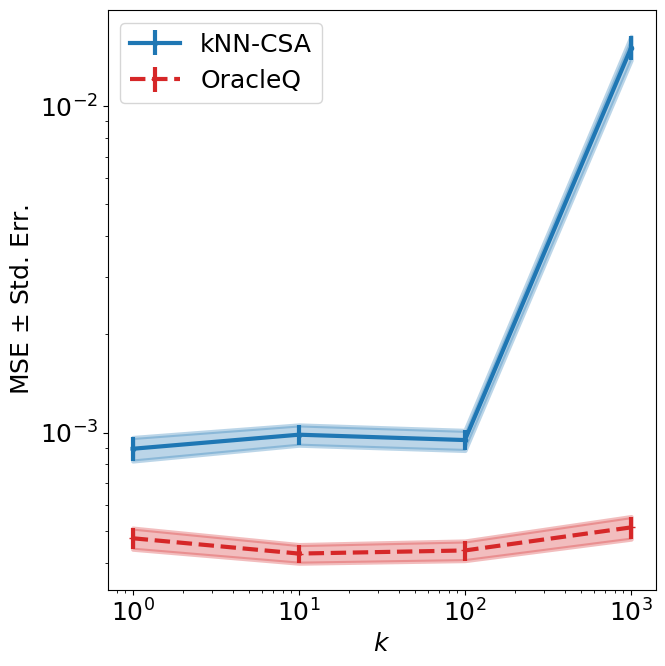
Figure 4: Proposed method with different $k$’s.

A.10 Limitation

Some papers show that the $k$-d tree slows down for high dimensional cases. One might want to use approximate nearest neighbors to overcome this issue. However, our theory assumes that the nearest neighbor method returns the exact nearest neighbors.

	Twonorm	Diabetes
1NN-S	0.055 (0.003)	3223 (283)
KMM-W	0.063 (0.005)	3107 (205)

Table 4: MSE for real-world datasets.

References

- Aminian et al. (2022) Aminian, G., M. Abroshan, M. Mahdi Khalili, L. Toni, and M. Rodrigues (2022, 28–30 Mar). An information-theoretical approach to semi-supervised learning under covariate-shift. In Proceedings of The 25th International Conference on Artificial Intelligence and Statistics, Volume 151 of Proceedings of Machine Learning Research, pp. 7433–7449. PMLR.
- Bentley (1975) Bentley, J. L. (1975). Multidimensional binary search trees used for associative searching. Communications of the ACM 18(9), 509–517.
- Blumenson (1960) Blumenson, L. (1960). A derivation of n-dimensional spherical coordinates. The American Mathematical Monthly 67(1), 63–66.
- Bogachev and Ruas (2007) Bogachev, V. I. and M. A. S. Ruas (2007). Measure theory, Volume 2. Springer Science & Business Media.
- Chen et al. (2022) Chen, L., M. Zaharia, and J. Y. Zou (2022). Estimating and explaining model performance when both covariates and labels shift. In Advances in Neural Information Processing Systems, Volume 35, pp. 11467–11479. Curran Associates, Inc.
- Clémençon and Portier (2018) Clémençon, S. and F. Portier (2018). Beating monte carlo integration: A nonasymptotic study of kernel smoothing methods. In International Conference on Artificial Intelligence and Statistics, pp. 548–556. PMLR.
- de Mathelin et al. (2021) de Mathelin, A., M. Atiq, G. Richard, A. de la Concha, M. Yachouti, F. Deheeger, M. Mougeot, and N. Vayatis (2021). ADAPT : Awesome Domain Adaptation Python Toolbox. arXiv:2107.03049 [cs.LG].
- Delyon and Portier (2016) Delyon, B. and F. Portier (2016). Integral approximation by kernel smoothing. Bernoulli 22(4), 2177–2208.
- Dua and Graff (2017) Dua, D. and C. Graff (2017). UCI machine learning repository.
- Friedman et al. (1977) Friedman, J. H., J. L. Bentley, and R. A. Finkel (1977). An algorithm for finding best matches in logarithmic expected time. ACM Transactions on Mathematical Software (TOMS) 3(3), 209–226.
- Gretton et al. (2008) Gretton, A., A. Smola, J. Huang, M. Schmittfull, K. Borgwardt, and B. Schölkopf (2008, December). Covariate Shift by Kernel Mean Matching. In Dataset Shift in Machine Learning, pp. 131–160. The MIT Press.
- Huang et al. (2006) Huang, J., A. Gretton, K. Borgwardt, B. Schölkopf, and A. Smola (2006). Correcting sample selection bias by unlabeled data. In Advances in Neural Information Processing Systems, Volume 19. MIT Press.
- Kanamori et al. (2009) Kanamori, T., S. Hido, and M. Sugiyama (2009). A least-squares approach to direct importance estimation. Journal of Machine Learning Research 10(48), 1391–1445.
- Kpotufe and Martinet (2021) Kpotufe, S. and G. Martinet (2021). Marginal singularity and the benefits of labels in covariate-shift. The Annals of Statistics 49(6), 3299–3323.
- Le et al. (2013) Le, Q., T. Sarlós, A. Smola, et al. (2013). Fastfood—approximating kernel expansions in loglinear time. In Proceedings of the 30th International Conference on Machine Learning, Volume 28.
- Lee et al. (2013) Lee, D.-H. et al. (2013). Pseudo-label: The simple and efficient semi-supervised learning method for deep neural networks. In Workshop on Challenges in Representation Learning, ICML.
- Leluc et al. (2023) Leluc, R., F. Portier, J. Segers, and A. Zhuman (2023). Speeding up monte carlo integration: Control neighbors for optimal convergence. arXiv preprint arXiv:2305.06151.
- Mazaheri (2020) Mazaheri, B. (2020). Supplementary files for robustly correcting sampling bias using cumulative distribution functions. https://github.com/honeybijan/NeurIPS2020.
- Portier (2021) Portier, F. (2021). Nearest neighbor process: weak convergence and non-asymptotic bound. arXiv preprint arXiv:2110.15083.
- Scott (1992) Scott, D. (1992). Multivariate Density Estimation: Theory, Practice, and Visualization. John Wiley & Sons.
- Shimodaira (2000) Shimodaira, H. (2000). Improving predictive inference under covariate shift by weighting the log-likelihood function. Journal of Statistical Planning and Inference 90(2), 227–244.
- Sugiyama et al. (2007) Sugiyama, M., S. Nakajima, H. Kashima, P. v. Bünau, and M. Kawanabe (2007). Direct importance estimation with model selection and its application to covariate shift adaptation. In Advances in Neural Information Processing Systems 20, NIPS 2007, pp. 1433–1440.
- Sugiyama et al. (2008) Sugiyama, M., T. Suzuki, S. Nakajima, H. Kashima, P. von Bünau, and M. Kawanabe (2008, December). Direct importance estimation for covariate shift adaptation. Annals of the Institute of Statistical Mathematics 60(4), 699–746.
- Truquet (2011) Truquet, L. (2011). On a nonparametric resampling scheme for markov random fields. Electronic Journal of Statistics 5, 1503–1536.
- Uhlmann (1966) Uhlmann, W. (1966). Vergleich der hypergeometrischen mit der binomial-verteilung. Metrika 10, 145–158.
- Van der Vaart (2000) Van der Vaart, A. W. (2000). Asymptotic Statistics, Volume 3. Cambridge University Press.
- Wang (2023) Wang, K. (2023, March). Pseudo-Labeling for Kernel Ridge Regression under Covariate Shift. arXiv:2302.10160 [cs, math, stat].
- Williams and Seeger (2000) Williams, C. K. I. and M. Seeger (2000). Using the Nyström Method to Speed up Kernel Machines. In Advances in Neural Information Processing Systems, Volume 13 of NIPS 2000, pp. 661–667. MIT Press.
- Yamada et al. (2013) Yamada, M., T. Suzuki, T. Kanamori, H. Hachiya, and M. Sugiyama (2013, May). Relative Density-Ratio Estimation for Robust Distribution Comparison. Neural Computation 25(5), 1324–1370.
- Zhang et al. (2021) Zhang, T., I. Yamane, N. Lu, and M. Sugiyama (2021, June). A One-Step Approach to Covariate Shift Adaptation. SN Computer Science 2(4), 319.