RANRAC: Robust Neural Scene Representations via Random Ray Consensus

Abstract

We introduce RANRAC, a robust reconstruction algorithm for 3D objects handling occluded and distracted images, which is a particularly challenging scenario that prior robust reconstruction methods cannot deal with. Our solution supports single-shot reconstruction by involving light-field networks, and is also applicable to photo-realistic, robust, multi-view reconstruction from real-world images based on neural radiance fields. While the algorithm imposes certain limitations on the scene representation and, thereby, the supported scene types, it reliably detects and excludes inconsistent perspectives, resulting in clean images without floating artifacts. Our solution is based on a fuzzy adaption of the random sample consensus paradigm, enabling its application to large scale models. We interpret the minimal number of samples to determine the model parameters as a tunable hyperparameter. This is applicable, as a cleaner set of samples improves reconstruction quality. Further, this procedure also handles outliers. Especially for conditioned models, it can result in the same local minimum in the latent space as would be obtained with a completely clean set. We report significant improvements for novel-view synthesis in occluded scenarios, of up to 8dB PSNR compared to the baseline.

1 Introduction

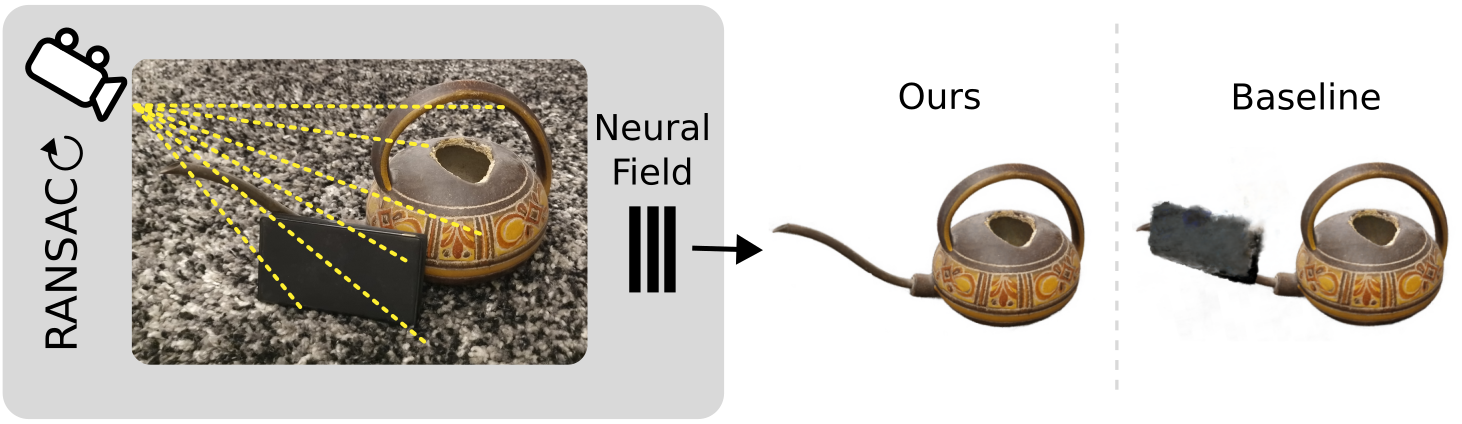
Figure 1: We propose a robust algorithm for 3D reconstruction from occluded input perspectives that is based on the random sampling of hypotheses. Our algorithm is general and we demonstrate the use for single-shot reconstruction using light field networks or multi-view reconstruction using NeRF. In these cases, it successfully removes the artifacts that normally occur due to occluded input perspectives.

3D reconstruction is a classical task in computer vision and computer graphics, which has attracted research for decades. It offers numerous applications, including autonomous systems, entertainment, design, advertisement, cultural heritage, VR/AR experiences or medical scenarios. In recent years, neural scene representations and rendering techniques [51, 44], including light field networks (LFN) [41] and neural radiance field (NeRF) [29] have demonstrated great performance in single-view and multi-view reconstruction tasks. The key to the success of such techniques is the coupling of differentiable rendering methods with custom neural field parametrizations of scene properties. However, a common limitation of neural scene reconstruction methods is their sensitivity to inconsistencies among input images induced by occlusions, inaccurately estimated camera parameters or effects like lens flares. Despite the use of view-dependent radiance representations to address view-dependent appearance changes, these inconsistencies severely impact local density estimation, resulting in a poor generalization to novel views.

To increase the robustness to potential distractors within the training data, Sabour et al. [38] recently introduced the use of robust losses in the context of training unconditioned NeRF, where distractors in the training data were modeled as outliers of an optimization problem. However, the adaptation of this approach to conditioned neural fields (e.g., pixelNeRF [52]) is not obvious, as no optimization takes place during inference, and the input data is constrained to only a few views. Achieving robustness to data inconsistencies is a well-analyzed problem in computer vision, covered not only by the aforementioned robust loss functions [1], but also other strategies, like the random sample consensus (RANSAC) paradigm [15]. The latter is widely employed for fitting models to outlier-heavy data. The underlying idea is to randomly select subsets of the data to form potential models, evaluating these models against the entire dataset, and identifying the subset that best fits the majority of the data, while disregarding outliers. Despite being the state-of-the-art solution to many challenges, RANSAC-based schemes are particularly favoured for the fitting of analytical models with a relatively small amount of tuneable parameters. In this paper, we direct our attention to achieving robustness against inconsistencies and occlusions in the observations by using a novel combination of neural scene representation and rendering techniques with dedicated outlier removal techniques such as RANSAC [15]. While downweighting the influence of distractors based on robust losses [1, 38] can affect clean samples, representing details, we aim at improving robustness to distractors by only removing the influence of outliers. To this extent, we integrate a RANSAC-based scheme to distinguish inliers and outliers in the data and the inlier-based optimization of the neural fields; a stochastic scenario characterized by a large-scale, data-driven model that exceeds RANSAC’s classical convergence expectations. Instead of guaranteeing convergence to a clean sample set based on a minimal number of samples, we aim for a feasible (cleaner) sample set using a tuneable amount of samples. The proposed algorithm exhibits robustness and versatility, accommodating a wide range of neural fields-based reconstruction methods.

Our method inherits the strengths of RANSAC, such as the ability to handle various classes of outliers without relying on semantics. Yet, it also inherits the need for sufficiently clean samples and the reliance on an iterative scheme. In practice, the first condition is often fulfilled because typically only some of the perspectives are affected by inconsistencies. We validate our approach using synthetic data, focusing on the task of multi-class single-shot reconstruction with LFNs [41], and observe significant quality improvements over the baseline in the presence of occlusions. Furthermore, we showcase robust photo-realistic reconstructions of 3D objects using unconditioned NeRFs from sequences of real-world images in the presence of distractors. In comparison to RobustNeRF [38], we use all available clean data, hence improving the reconstruction quality for single-object scenes.

Our key contributions are:

• a robust RANSAC-based reconstruction method applied to multi-class single-shot reconstruction via LFNs, with demonstrated applicability to other neural fields, supporting complex data-driven models;

• an analysis of the implication to RANSAC’s hyperparameters and theoretical convergence expectations, and the experimental study of their effect;

• a qualitative/quantitative evaluation of our algorithm.

2 Related Work

Among the vast literature on neural fields, the seminal work of Mildenhall et al. [29] opened many avenues in the computer vision community. It contributed to state-of-the-art solutions for novel view synthesis and 3D reconstruction that have been covered in respective surveys [51, 44]. Noteworthy is the more recent contribution of instant neural graphics primitives (iNGP) [31], which uses a hash table of trainable feature vectors alongside a small network for representing the scene. iNGP achieved major run-time improvements, thereby enhancing the feasibility of practical applications for neural fields.

Baseline models are highly sensitive to imperfections in the input data, which led to many works on robustness enhancements of neural fields; addressing a reduced amount of input views [32, 21, 17, 52], errors in camera parameters [25, 19, 53, 4], variations in illumination conditions across observations [28, 42], multi-scale image data [50, 2, 3], and the targeted removal of floating artifacts [47, 48, 33].

Fewer works solve the reconstruction task in the presence of inconsistencies between observations. Bayes’ Rays [16] provides a framework to quantify uncertainty of a pretrained NeRF by approximating a spatial uncertainty field. It handles missing information due to self-occlusion or missing perspectives well, but cannot deal with inconsistencies caused by noise or distractors. Similarly, NeuRay [26] only supports missing, but not inconsistent information.

Naive occlusion handling via semantic segmentation requires the occluding object types to be known in advance [28, 37, 43, 36, 46]. Solutions to learn semantic priors on transience exist [23] but separating occlusions via semantic segmentation without manual guidance is ill posed.

Occ-NeRF [54] considers any foreground element as occlusion and removes them via depth reasoning, but their removal leaves behind blurry artifacts. Alternatively, some methods do not remove dynamic distractors, but reconstruct them together with the rest of the scene using time-conditioned representations [27, 49, 34, 9].

Like us, RobustNeRF [38] considers input-image distractors as outliers of the model optimization task. It employs robust losses improved via patching to preserve high-frequency details. It does not make prior assumptions about the nature of distractors, nor does it require preprocessing of the input data or postprocessing of the trained model. Nevertheless, their method comes at the cost of a reduced reconstruction quality in undistracted scenes. Furthermore, their method is limited to unconditioned models that overfit to a single scene. A generalization to conditioned NeRFs, such as pixelNeRF [52], is not obvious, as no further optimization takes place during inference.

Conditioned neural fields offer a distinct advantage in their ability to generalize to novel scenes by leveraging knowledge acquired from diverse scenes during learning. This results in a more robust model that requires as few as one input view for inference, showcasing the efficiency and adaptability of the approach. Contrary to PixeNeRF [52], which relies on a volumetric parametrization of the scene, demanding multiple network evaluations along the ray, Light Field Networks [41], which succeed Scene Representation Networks [40], take a different approach. LFNs represent the scene as a 4D light field, enabling a more efficient single evaluation per ray for inference. The network takes as input a ray represented in Plücker coordinates and maps it to an observed radiance, all within an autoencoder framework used for conditioning.

None of the mentioned methods can deal with occlusions in single-shot reconstruction and no prior work exists on robust LFNs or robustness of other conditioned neural fields for single-shot reconstruction, which we address via the RANSAC paradigm [15]. Since its introduction in 1981, RANSAC has gained attention for fitting analytical models with a small number of parameters, such as homography estimation in panorama stitching [7]. Among the few direct applications of classical RANSAC to larger models is robust morphable face reconstruction [13, 14]. Other common expansions and applications include differentiable RANSAC [6] for camera parameter estimation in a deep learning pipeline, locally optimized RANSAC [11] to account for the requirement of a descriptive sample set, and adaptive real-time RANSAC [35].

3 Method

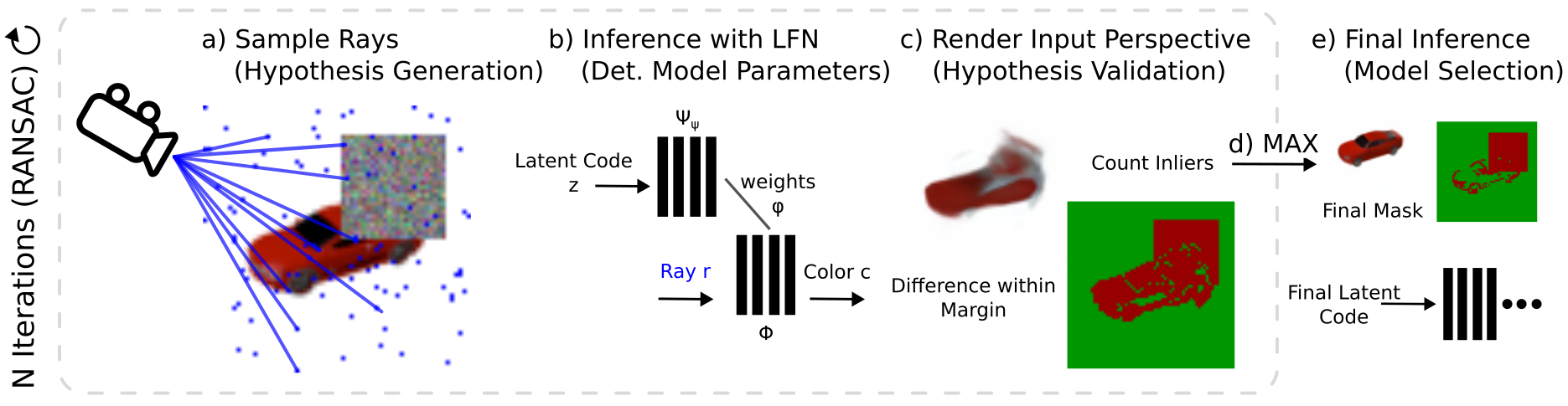
Figure 2: The RANRAC algorithm for LFNs samples random hypotheses by selecting a set of random samples from the given perspective (a), and inferring the latent representation of these rays using the autodecoder of a pretrained LFN (b). The obtained light field is then used to predict an image from the input perspective (c). Based on this prediction, confidence in the random hypothesis is evaluated via the Euclidean distance between the predicted ray colors and the remaining color samples of the input image. The amount of samples which are explained by each hypothesis up to some margin are used to determine the best hypothesis (d). All samples explained by the selected hypothesis are used for a final inference with the LFN to obtain the final model and latent representation (e).

First, we recap RANSAC, its theoretical convergence and hyperparameters, and the required adaptions for its application to high-dimensional data-driven models. Based hereon, we formulate a robust single-shot algorithm using LFNs for 3D reconstruction from images with occlusions. Finally, we discuss the generalization to other neural fields with a demonstration of a robust photo-realistic multi-shot reconstruction with NeRFs.

3.1 Parameters and Convergence of RANSAC

Classical RANSAC [15, 10, 12] follows an iterative process. Initially, a minimal set of samples is randomly selected to determine the model parameters, known as the hypothesis generation phase. Then, the hypothesis is evaluated by assessing the number of observations it explains, within a specified margin. These steps are repeated until the best hypothesis is chosen to constitute the consensus set, which comprises all of its inliers.

This paradigm cannot be directly applied to complex models such as neural fields, as a significant amount of samples is required to obtain decent initial model parameters and additional clean samples improve the quality further. This imposes a challenge regarding the expected amount of clean initial sample sets, $S_{clean}$:

$$\mathbb{E}[\#S_{clean}]=N*\prod_{m=1}^{M}\frac{s_{img}-s_{img}^{occ}-m}{s_{img}-m},$$ (1)

where $s_{img}$ denotes the total amount of samples (e.g., image pixels), $s_{img}^{occ}$ represents the occluded samples, and $N$/$M$ are the number of iterations/samples. The expected amount exponentially decreases with the initial number of samples.

The samples and respective requirements for analytic and data-driven models vary a lot. The effect of individual samples is less traceable in data-driven models and the information entropy varies more significantly across samples. When using a model that projects onto a latent space, some very atypical outliers do not show an effect at all if the latent space is not expressive enough to explain them in an overall loss-reducing way, yet, outliers close to the object or its color, or larger chunks of outliers, will usually be distracting. At the same time, samples of small-scale high-frequency details are important for the reconstruction and contain a lot of information, whereas multiple samples of larger-scale lower-frequency details contribute much less. The amount of initial samples for the hypothesis generation becomes a tunable hyperparameter trading initial reconstruction quality for likelihood of finding desired sample sets. This invalidates the classical convergence idea [10, 12]

$$N\geq\frac{\log(1-p)}{\log(1-t^{M})}$$ (2)

where the RANSAC iterations $N$ are chosen such that at least one clean sample set is found with a probability $p$, given the expected ratio of clean samples $t$ and the amount of initial samples $M$. Not only a clean sample set has to be found, but one that captures all important details. At the same time, a completely clean sample set is not required at all, as long as the contained outliers are not represented by the local minimum of the latent space or the model itself, depending on the concrete scene representation.

3.2 Robust Light Field Networks

In the following, we propose a fast and robust single-shot multi-class reconstruction algorithm based on LFNs [41]. LFNs are globally conditioned, meaning that the supported subset of 3D consistent scenes is represented by a single global latent vector. Therefore, when the latent space is not expressive enough to represent object and distractor correctly, large inconsistencies cause global damage instead of local artifacts.

Our algorithm first generates hypothesis sets via random sampling and infers these sets with a pretrained LFN. The validity of the hypotheses is then checked by determining the amount of consistent observations under every hypothesis. Based on this, the observations consistent with the strongest hypothesis are used to determine the parameters of the final model. The steps are described in more detail below.

1. Hypothesis Consensus Set: Given the input image $I$ as a set of pixel color values $\bm{\mathit{c}}_{i}$, and the intrinsic and extrinsic camera parameters, the set of rays $R$ – one ray $\bm{\mathit{r}}_{i}$ for every pixel – represented by Plücker coordinates, is generated. In the first step, $N$ initial consensus sets $S_{n}$ are drawn using a uniform distribution, where each consensus set consists of $M$ random samples:

   $$(\bm{\mathit{c}}_{n}^{m},\bm{\mathit{r}}_{n}^{m})\in_{R}\{(\bm{\mathit{c}}_{i},\bm{\mathit{r}}_{i})\mid\bm{\mathit{c}}_{i}\in I,\bm{\mathit{r}}_{i}\in R\}$$ (3)

   where $n\in\{1,\dots,N\}$, $m\in\{1,\dots,M\}$, and $\in_{R}$ denotes a uniform random drawing from the set without replacement.

2. Hypothesis Inference: The autodecoder of a pretrained LFN (Sec. 2), is used to infer the latent codes $\bm{\mathit{z}}_{n}$ for each of the initial sample sets in parallel.

   $$\{\bm{\mathit{z}}_{n}\}=\mathop{\mathrm{argmin}}\limits_{\{\bm{\mathit{z}}_{n}\}}\sum_{n}\sum_{m}\\ \lVert\Phi(\bm{\mathit{r}}_{n}^{m}\mid\Psi_{\psi}(\bm{\mathit{z}}_{n}))-\bm{\mathit{c}}_{n}^{m}\rVert_{2}^{2}+\lambda_{lat}\lVert\bm{\mathit{z}}_{n}\rVert_{2}^{2}$$ (4)

   An exponential learning rate schedule speeds up the inference. The inferred latent codes form the hypotheses.

3. Hypothesis Prediction: Each of the hypotheses is used to render an entire image $I_{n}^{pred}$ from the perspective of the input image, each consisting of the pixel color values $\bm{\mathit{c}}_{n,i}^{pred}=\Phi(\bm{\mathit{r}}_{i}\mid\Psi_{\psi}(\bm{\mathit{z}}_{n}))$ , using again the set of rays $R=\{\bm{\mathit{r}}_{i}\}$ obtained from the camera parameters. The rendered pixels resemble the predictions for the remaining observations under each hypothesis.

4. Hypothesis Validation: The obtained predictions are compared to the input image to validate the hypothesis. For each pixel in each predicted image, we calculate the Euclidean distance in color space: $e_{n,i}=\lVert\bm{\mathit{c}}_{n,i}^{pred}-\bm{\mathit{c}}_{i}\rVert_{2}.$ For each image, using these distances, we collect, up to some margin $\epsilon$, the observations explained by the model (inliers) : $S_{n}^{inlier}=\{(\bm{\mathit{c}}_{i},\bm{\mathit{r}}_{i})\mid e_{n,i}<\epsilon\}$

5. Model Selection: We select the best hypothesis sample set $S_{best}$ based on the number of inliers $\#S_{n}^{inlier}$. The model is inferred once more, similar to the second step, to obtain the final latent code $z_{cons}$. The inference is based on the final consensus set $S_{cons}=S_{best}\cup S_{best}^{inlier}$, the initial sample set of the strongest hypothesis $S_{best}$ together with all its inliers $S_{best}^{inlier}$.

The final output consists of both the latent code $z_{cons}$ and the final consensus set $S_{cons}$ of the selected model, and can be used to render arbitrary new perspectives.

3.3 Robust Neural Radiance Fields

As an example for the generality of our solution, we demonstrate its application to Neural Radiance Fields. Most formulations of neural scene representations are based on a set of rays and thereby open for ray-based subsampling and inference. However, the sample space has to be chosen with care to enable practical convergence within reasonable amounts of time.

Unconditioned neural radiance fields are fit to a single scene based on a set of observations. As they support view-dependent radiance, one might expect inconsistencies in the input observations to only have an effect on specific perspectives. However, the density is only spatially parametrized, and therefore, inconsistencies lead to significant ghosting and smearing artifacts in more than just the inconsistent perspective. This can once again be leveraged in the hypothesis validation.

A decent fit of a neural radiance field requires a large set of rays, orders of magnitude higher than for LFNs. This requirement makes a sampling in ray space infeasible, due to the exponential decay of the expected amount of clean sample sets. Therefore, we propose to sample in observation space. The reconstructions of NeRF commonly start to get usable, even though not completely artifact free, at around 20–25 observations, while additional perspectives keep improving the reconstruction quality [29, table 2]. Therefore, sampling observations results in a sampling domain with reasonably sized sample sets. Other choices of the sampling space are possible as well if they are desirable for a specific domain, as long as the size of the initial sample set remains feasible.

The chosen sample space also requires an adaption of the hypothesis evaluation. We propose a two-step evaluation, where, for every predicted perspective, the pixel inliers are counted and used to label the perspective itself.

In the first step, the rendered images $I^{pred}_{i}$ under the hypothesis model are compared to the input images $I_{i}$ of the observations not used for the reconstruction. For each pixel $\bm{\mathit{p}}^{pred}_{i,k}$ in each image, the Euclidean distance in color space $e_{i,k}$ to the corresponding pixel $\bm{\mathit{p}}_{i,k}$ of the input image is calculated.

$$e_{i,k}=\lVert\bm{\mathit{p}}_{i,k}^{pred}-\bm{\mathit{p}}_{i,k}\rVert_{2}$$ (5)

Using these distances, for each image, the pixels explained by the hypothesis model, up to some margin $\epsilon_{pix}$, are counted.

$$P_{i}^{\#}=\#\{\bm{\mathit{p}}^{pred}_{n,k}\mid e_{n,i}<\epsilon_{pix}\}$$ (6)

In the second step, based on these per-image inlier counts, the entire images are labeled as inlier or outlier, once again based on some margin $\epsilon_{img}$ and the set of inlier observations is collected.

$$S^{inlier}_{n}=\{(I_{i},E_{i},K_{i})\mid P_{i}^{\#}>\epsilon_{img}\}$$ (7)

The binary metric for pixels makes sure that smaller mispredictions (due to, e.g., view-dependent lighting effects) do not introduce noise into the evaluation. Only larger mispredictions belonging to actual artifacts shall be counted. Our binary choice of an entire image ensures that only perspectives containing significant artifacts are considered outliers, while smaller perturbations are maintained.

The sampling of observations introduces the theoretical limitation of not having enough clean observations in the input data. The method is therefore not applicable to scenarios where every input perspective contains strong distractors, which are arguably rare in practical captures. In return, our method is not limited to specific kinds of inconsistencies, and is robust to arbitrarily heavy distractions or inconsistencies in the impure perspectives. In fact, our method even benefits from stronger inconsistencies, as they make the affected perspectives easier to separate from the clean ones.

3.4 Hyperparameters

For LFNs, the amount of initial samples and random hypotheses to evaluate (iterations), are determined experimentally. Without fine-tuning per class, the experimentally determined parameters are 90 initial samples and 2000 iterations, which supersedes the theoretical value for a convergence because the latent space introduces an intrinsic robustness. Please refer to the supplementary material for further experimental results.

For NeRFs, the values behave more natural and the amount of perspectives required for a meaningful, not completely artifact-free fit of the model lies around 25 observations [29, table 2]. With fewer samples, more artifacts are introduced that get harder to separate from the ones caused by inconsistencies, and the samples get more dependent on being evenly spaced. For real-world captures with 10% inconsistent perspectives, as few as 50 iterations are sufficient.

The inlier margin for LFN balances the amount of slight high-frequency variations that are being captured and the capability of separating outliers that are similar to the object. A margin of 0.25 in terms of the Euclidean distance of the predicted colors to the input samples in an RGB color space normalized to the range $(-1,1)$ has been found to be optimal.

For the NeRFs, with their color space normalized to $(0,1)$, a pixel margin of $\epsilon_{pix}=0.15$ in terms of Euclidean distance worked well for the determination of actual artifacts. We consider an observation an inlier based on a margin of 98% pixel inliers, which proved to be a good choice to separate minor artifacts (due to the sparse sampling) from artifacts caused by actual inconsistencies. For different datasets or inconsistencies, these values could be fine-tuned.

4 Implementation & Preprocessing

For LFNs, we build on top of the original implementation [41], with a slight adaptation to enable a parallel sub-sampled inference. We furthermore use the provided pretrained multi-class model. The camera parameters are known. For efficiency reasons, the steps of the algorithm are not performed iteratively, but multiple hypotheses are validated in parallel, leading to a total runtime of about a minute. To further speed up the inference, an exponential learning rate schedule is used for the auto-decoding.

For the robust reconstruction of objects from lazily captured real-world data, one has to estimate the camera parameters and extract foreground masks before applying the algorithm. For the estimation of the camera parameters, we used the COLMAP structure-from-motion package [39]. We extracted foreground masks using Segment Anything [22]. However, only foreground masks, containing the objects and the occlusions, are extracted. Segment Anything is not capable of removing arbitrary occlusions in an automatized way. After these preprocessing steps, the robust reconstruction algorithm can be applied as described. Erroneous estimates of the camera parameters or foreground masks are excluded by our algorithm, thus making the entire reconstruction pipeline robust.

Our algorithm is not limited to a specific NeRF implementation. The chosen sampling domain eases integration into arbitrary existing NeRF implementations, which commonly expect images instead of unstructured ray sets. However, using a fast NeRF variant is advantageous when applying an iterative scheme. We used the instant NGP implementation [31] of the instant NSR repository [18], which includes some accelerations [30, 24]. Other, (specifically fast) variants are likely good choices as well. Antialiased and unbounded, but slow variants, such as MipNeRF360 [3], are not feasible.

5 Experiments

Metric	Model	Bench	Boat	Cabinet	Display	Lamp	Phone	Rifle	Sofa	Speaker	Table
PSNR$\uparrow$	RANRAC	19.21	22.92	21.92	17.65	19.99	18.45	21.35	21.61	20.7	20.44
	LFN	17.89	19.2	20.5	18.85	19.09	17.81	18.46	20.12	19.99	20.29
SSIM$\uparrow$	RANRAC	0.767	0.858	0.801	0.699	0.764	0.75	0.853	0.805	0.761	0.784
	LFN	0.724	0.791	0.767	0.73	0.748	0.726	0.795	0.775	0.743	0.777

Table 1: RANRAC obtains a significant quantitative improvement in PSNR and SSIM (higher is better) compared to the baseline. We compare RANRAC to vanilla LFNs for the 13 largest ShapeNet classes other than plane, car, and chair, which are analyzed in more detail in Figs. 4 and 5. The results are based on a moderate amount of occlusion of approximately 25% object occlusion and about 5% image occlusion. The reported results are conservative, as higher amounts of image occlusion result in a more significant performance increase (Fig. 4). No hyperparameters tuning has been performed for these classes; the same configuration obtained from the analysis of the other three classes is used. Our performance improvement is most significant for classes that can be well reconstruted by LFNs under clean conditions and less significant for classes that already present a challenge to LFNs in general. The only outlier is the display class, on which LFNs struggle the most on [41], even in unoccluded scenarios. This implies that it is not consistently represented in the latent space. The robust reconstruction amplifies this effect by reducing the samples to a consistent set.

5.1 Baseline, Datasets & Occlusions

We benchmark against the original LFN implementation of Sitzmann et al. [41] as baseline, as there are no other robust methods for LFNs or conditioned neural fields, nor are there methods for robust single-shot multi-class reconstruction in general. Furthermore, we use the same pretrained LFN for the baseline and for the application of our method. The LFN is pretrained on the thirteen largest ShapeNet classes [8].

We provide a detailed qualitative and quantitative performance comparison under different amounts of occlusion for three representative classes (plane, car, and chair), while just stating reconstruction performance in a fixed environment without additional tuning of the hyperparameters for the others. The plane class is mostly challenging due to the low-frequency shape, while the car class contains a lot of high-frequency color details. The chair class represents shapes that are generally problematic for vanilla LFNs, even without occlusions. We provide a complementing analysis of the hyperparameters in the supplementary material. If not stated otherwise, we evaluate using fifty randomly selected images of the corresponding class. All comparisons use the same images.

The occlusions are created synthetically. They consist of consecutive random patches with random dimensions and position, while controlling two metrics of occlusion: Image occlusion and object occlusion. The former is the naive ratio of occluded over total pixels. The latter are the occluded pixels on the object compared to the total pixels covered by the object. We use both metrics to take the vastly different information entropy of samples across the image into account. Occlusions that do not cover the object at all, do not cause any information loss and should not fall into the same category as an occlusion that covers the actual object.For further details on the generation of the synthetic occlusions, please refer to the supplemental.

RobustNeRF [38], targets unbounded scenes with multiple objects and small amounts of distractors in every perspective. In comparison, our RANSAC-based approach deals well with single-object reconstruction, even with heavy occlusions, as long as enough clean perspectives are available. As their dataset reflects the algorithm’s properties, we cannot provide a fair comparison. Instead, we demonstrate the applicability using a custom dataset of a single object with a certain amount of deliberately occluded perspectives. Furthermore, we implement the robust losses [38] on the same NeRF variant as RANRAC to provide a fair comparison of the method’s robustness, independent of the NeRF flavor. For further details on the implementation, please refer to the supplementary material.

5.2 Evaluation

For LFNs, our approach leads to a significant improvement in occluded scenarios of up to 8dB in PSNR and a similarly strong improvement for the SSIM. The improvement is most significant in heavily distracted scenarios (Fig. 4). In clean scenarios a slight performance penalty can be observed, but even with small amounts of object occlusion (information loss), our algorithm outperforms the competitors, leading to numerically better results up to $50\%$ information loss (Fig. 5).

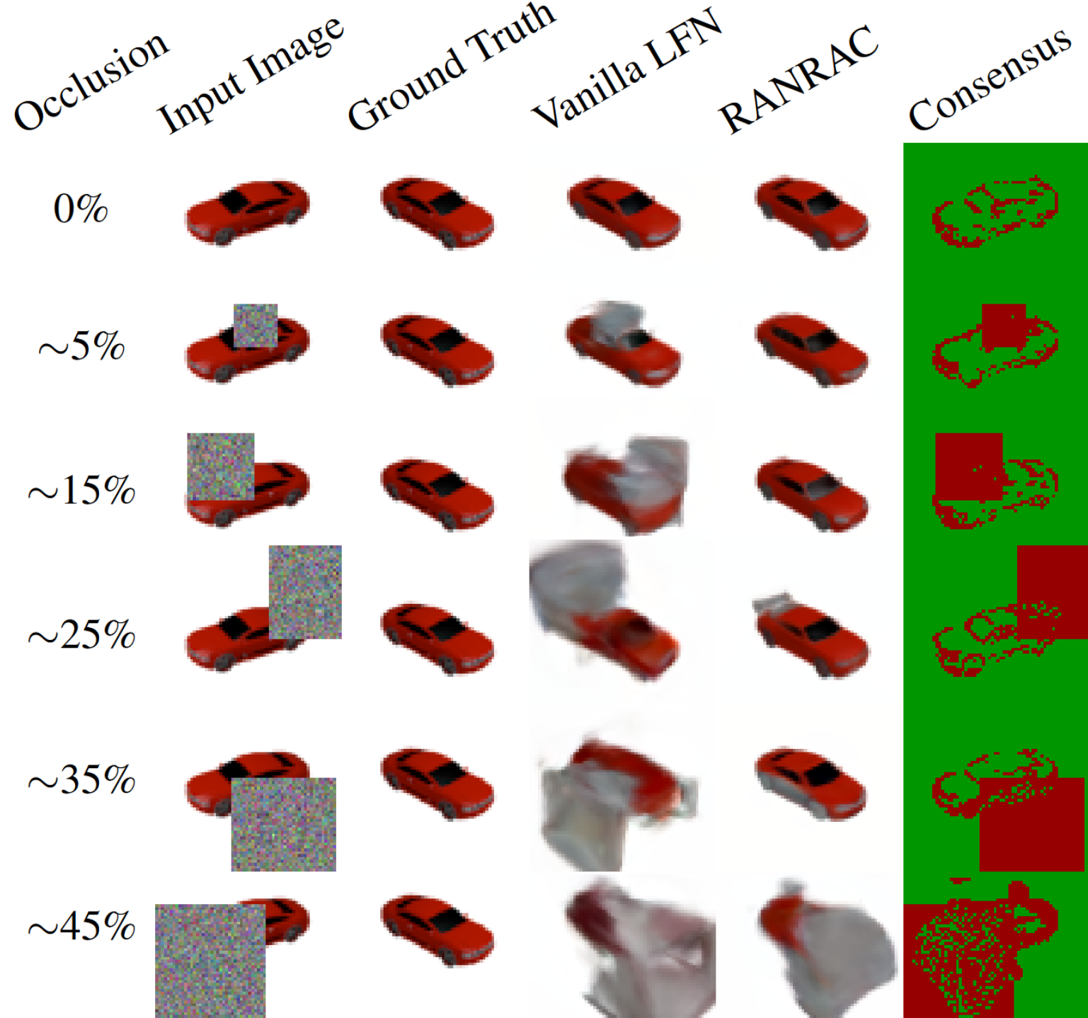
Figure 3: We show the qualitative effect of occlusion increase on the same observation for the reconstruction of a novel view. Reconstructions of LFNs break early globally but RANRAC provides a very decent reconstruction, only slowly introducing minor local (and natural/comprehensible) artifacts for completely hidden object parts. In the right column, we show the obtained consensus set, used for the final reconstruction (green inliers, red outliers).

The effect is not only measurable, but also well visible (Fig. 3). Increasing amounts of occlusion slowly introduce local artifacts into our reconstruction while preserving a reasonable shape estimate even for larger amounts of occlusion. In contrast, the reconstruction of LFNs breaks rather early in a global fashion. Still, our consensus set (Figs. 3 and 6), reveals that some high-frequency details were wrongfully excluded, explaining the slight performance decrease on clean images.

Figure 4: RANRAC (solid lines) leads to a quantitative improvement in PSNR and SSIM (higher is better) for occluded inputs compared to vanilla LFNs (dashed lines). The same hyperparameter configuration and LFN is used for all classes. The amount of image occlusion is increased, while the object occlusion is kept at about 25%. For the car class, a large improvement is observed over the entire occlusion spectrum. For the plane class the improvement is similarly significant, but absolute performance degenerates a bit sooner. This stems from the smaller object size and the related faster occlusion-to-object increase when increasing image occlusions. For the chair class, the improvement is less significant but the structural similarity is preserved for much longer.

In general, the benefit of RANRAC is best observable for classes that can be well described by LFNs, as evidenced by the lower improvements the chair class exhibits, compared to the plane and car class. The same effect is visible in the quantitative evaluation on the other classes without additional tuning (Tab. 1).

Figure 5: The quantitative improvement in PSNR and SSIM (higher is better) of RANRAC (solid lines) is significant compared to vanilla LFNs (dashed lines). The same hyperparameter configuration and LFN is used for all classes. The amount of object occlusion is increased, while image occlusion is constantly kept low to observe the isolated effect. For the plane and car class the reconstruction quality is resilient to information loss up to $\sim$50%, where the decrease gains momentum. With the low amounts of image occlusion, the improvement is not significant for the chair class (consistent to Fig. 4).

Input Image	G. Truth	Vanilla LFN	RANRAC	Consensus

Figure 6: Qualitative results of RANRAC compared to LFNs for novel view synthesis on different classes. The right column shows the corresponding consensus sets (green inlier, red outlier)

The application to NeRF shows the discriminative capabilities of RANRAC. For the mildly occluded scene, all distracted and undisctracted perspectives are detected as such (Tab. 2) and the reconstruction is therefore equivalent to a reconstruction from a completely clean set. This is a major advantage over RobustNeRF, where the reconstruction performance, even on clean sets, is slightly degraded. For heavier distracted scenes, RANRAC still labels nearly all perspectives correctly, successfully removes the artifacts (Fig. 7), and significantly improves the perceived quality. For object reconstruction, the performance of RANRAC is at least on par with RobustNeRF (Tab. 3).

		Consensus Mild
		Inlier	Outlier	$\Sigma$
Truth	Inlier	108	0	108
	Outlier	0	12	12
	$\Sigma$	108	12	120

		Consensus Heavy
		Inlier	Outlier	$\Sigma$
	Inlier	105	3	108
	Outlier	2	21	23
	$\Sigma$	107	24	131

Table 2: The confusion matrices of RANRAC on the Watering Pot dataset show the successful elimination of occluded perspectives from the reconstruction. On the milder distracted dataset (left), all outliers and inliers are correctly labeled, resulting in a completely clean set of images. For the heavier distracted dataset (right), a very decent reconstruction is still possible, as only a minor amount of inconsistencies is mislabeled.

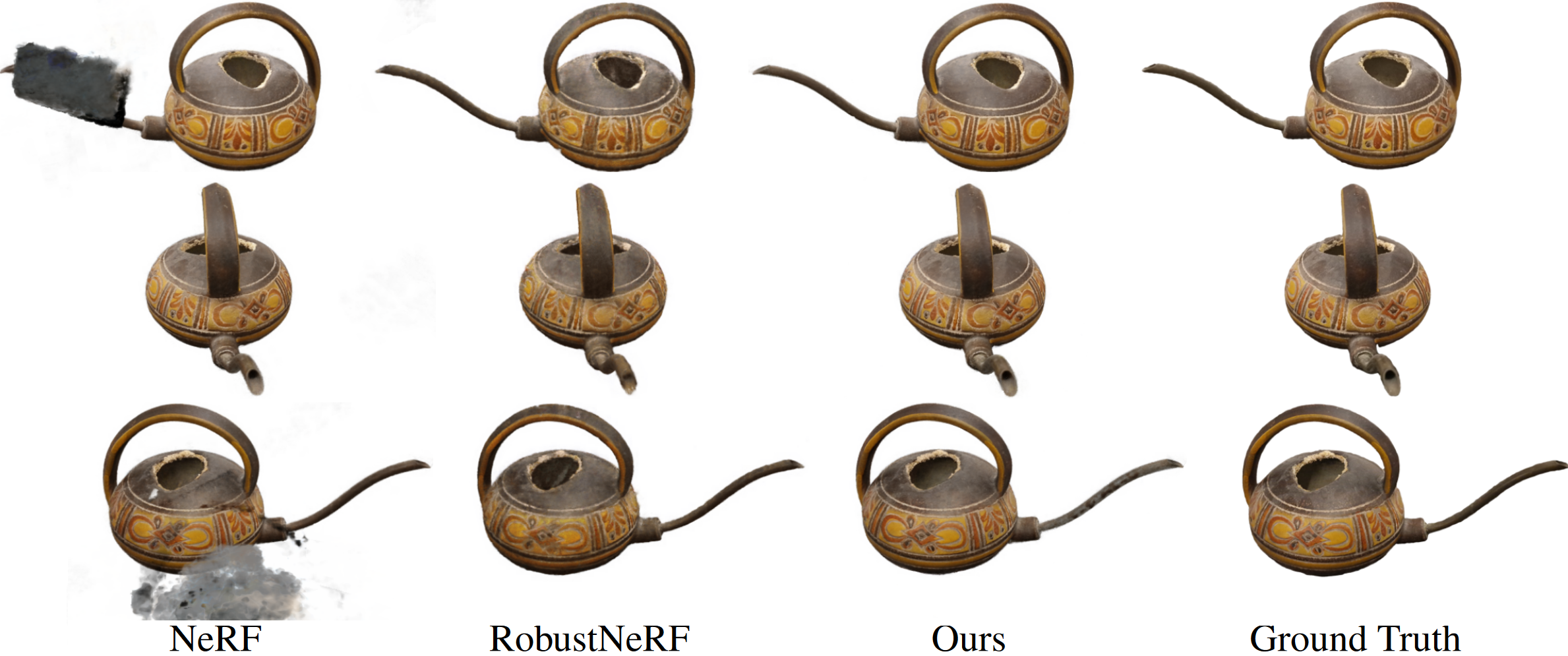
Figure 7: The occlusions lead to well-visible artifacts in the reconstructions of NeRF, these artifacts are completely removed by RANRAC.

	Mild			Heavy
	PSNR $\uparrow$	$P_{5}\uparrow$	$P_{1}\uparrow$	PSNR $\uparrow$	$P_{5}\uparrow$	$P_{1}\uparrow$
RANRAC	27.11	25.99	25.07	26.12	24.94	24.44
RobustNeRF	26.83	25.58	23.66	25.93	24.79	23.33
NeRF	26.65	22.61	16.74	25.36	18.47	15.97

Table 3: RANRAC achieves state-of-the-art object reconstruction from multiple views. We benchmark against RobustNeRF and NeRF (without any method for robustness) on the watering pot dataset. We compare with milder (10%) and heavier (17.5%) amounts of inconsistent perspectives. All three variants are built on top of instant-nsr for an isolated fair comparison of the robustness method. We report the average PSNR (higher is better) across views. As artifacts introduced by occlusions only contaminate some views, we also report the lower percentiles. RANRAC improves the PSNR significantly compared to NeRF and slightly compared to RobustNeRF.

Figure 8: Occlusion of important shape details (left, center) or perceptually-important elements (right) can lead to degenerate results. This mostly occurs for the chair class.

6 Limitations & Future Work

Our LFN approach shows strong performance for robust single-shot reconstruction. Future work might apply the method to other conditioned neural fields, based on a smart choice of the sampling domain, targeting photo-realism. Locally-optimized RANSAC [11] or DSAC [6], might be worth considering, too. One could also use importance sampling based on a prior instead of a uniform sampling, leveraging the unevenly distributed information entropy across samples. Neural sampling priors [5] or semantic segmentation might prove useful as well.

For unconditioned NeRFs, the iterations imply the use of a fast inferable NeRF variant, ruling out MipNeRF360 [3] and other high-quality variants for unbounded scenes. Further, foreground separation is a must, limiting this application of RANRAC to single-object reconstruction. The recent 3D Gaussian Splatting [20] raises optimism that this limitations may soon be lifted.

The only intrinsic problem of the RANRAC applied to NeRF is the requirement of sufficient clean perspectives, which could be lifted via NeRF variants that require fewer perspectives [32, 45] or by using different sampling domains.

7 Conclusion

We introduced a novel approach for robust single-shot reconstruction based on LFNs and inspired by RANSAC. The experimental evaluation showed a significant improvement of reconstruction quality in distracted and occluded scenarios, even for extreme cases. An advantageous property of our method is that it makes no assumption about the degree of distractions but robustly determines a clean sample set in an iterative process. As the generalization of existing techniques to conditioned fields is not obvious, we manged to close a relevant gap.

We further demonstrated photo-realistic multi-view reconstruction, showing that our methodology is widely applicable. In conjunction with future fast, high-quality neural fields our findings could be of particular value.

References

- Barron [2019] Jonathan T Barron. A general and adaptive robust loss function. In Proceedings of the IEEE/CVF Conference on Computer Vision and Pattern Recognition, pages 4331–4339, 2019.
- Barron et al. [2021] Jonathan T. Barron, Ben Mildenhall, Matthew Tancik, Peter Hedman, Ricardo Martin-Brualla, and Pratul P. Srinivasan. Mip-nerf: A multiscale representation for anti-aliasing neural radiance fields. In ICCV, 2021.
- Barron et al. [2022] Jonathan T. Barron, Ben Mildenhall, Dor Verbin, Pratul P. Srinivasan, and Peter Hedman. Mip-nerf 360: Unbounded anti-aliased neural radiance fields. In CVPR, 2022.
- Bian et al. [2023] Wenjing Bian, Zirui Wang, Kejie Li, Jia-Wang Bian, and Victor Adrian Prisacariu. Nope-nerf: Optimising neural radiance field with no pose prior. In CVPR, 2023.
- Brachmann and Rother [2019] Eric Brachmann and Carsten Rother. Neural-guided ransac: Learning where to sample model hypotheses. In ICCV, 2019.
- Brachmann et al. [2017] Eric Brachmann, Alexander Krull, Sebastian Nowozin, Jamie Shotton, Frank Michel, Stefan Gumhold, and Carsten Rother. Dsac-differentiable ransac for camera localization. In CVPR, 2017.
- Brown and Lowe [2007] Matthew Brown and David G Lowe. Automatic panoramic image stitching using invariant features. International Journal of Computer Vision, 74:59–73, 2007.
- Chang et al. [2015] Angel X. Chang, Thomas Funkhouser, Leonidas Guibas, Pat Hanrahan, Qixing Huang, Zimo Li, Silvio Savarese, Manolis Savva, Shuran Song, Hao Su, Jianxiong Xiao, Li Yi, and Fisher Yu. ShapeNet: An Information-Rich 3D Model Repository. Technical Report arXiv:1512.03012 [cs.GR], Stanford University — Princeton University — Toyota Technological Institute at Chicago, 2015.
- Chen et al. [2022] Xingyu Chen, Qi Zhang, Xiaoyu Li, Yue Chen, Ying Feng, Xuan Wang, and Jue Wang. Hallucinated neural radiance fields in the wild. In CVPR, 2022.
- Choi et al. [1997] Sunglok Choi, Taemin Kim, and Wonpil Yu. Performance evaluation of ransac family. Journal of Computer Vision, 24(3):271–300, 1997.
- Chum et al. [2003] Ondřej Chum, Jiří Matas, and Josef Kittler. Locally optimized ransac. In Pattern Recognition: 25th DAGM Symposium, Magdeburg, Germany, September 10-12, 2003. Proceedings 25, pages 236–243. Springer, 2003.
- Derpanis [2010] Konstantinos G Derpanis. Overview of the ransac algorithm. Image Rochester NY, 4(1):2–3, 2010.
- Egger et al. [2016] Bernhard Egger, Andreas Schneider, Clemens Blumer, Andreas Forster, Sandro Schönborn, and Thomas Vetter. Occlusion-aware 3d morphable face models. In BMVC, page 4, 2016.
- Egger et al. [2018] Bernhard Egger, Sandro Schönborn, Andreas Schneider, Adam Kortylewski, Andreas Morel-Forster, Clemens Blumer, and Thomas Vetter. Occlusion-aware 3d morphable models and an illumination prior for face image analysis. International Journal of Computer Vision, 126:1269–1287, 2018.
- Fischler and Bolles [1981] Martin A Fischler and Robert C Bolles. Random sample consensus: a paradigm for model fitting with applications to image analysis and automated cartography. Communications of the ACM, 24(6):381–395, 1981.
- Goli et al. [2023] Lily Goli, Cody Reading, Silvia Sellán, Alec Jacobson, and Andrea Tagliasacchi. Bayes’ Rays: Uncertainty quantification in neural radiance fields. arXiv, 2023.
- Guangcong et al. [2023] Guangcong, Zhaoxi Chen, Chen Change Loy, and Ziwei Liu. Sparsenerf: Distilling depth ranking for few-shot novel view synthesis. ICCV, 2023.
- Guo [2022] Yuan-Chen Guo. Instant neural surface reconstruction, 2022. https://github.com/bennyguo/instant-nsr-pl.
- Jeong et al. [2021] Yoonwoo Jeong, Seokjun Ahn, Christopher Choy, Anima Anandkumar, Minsu Cho, and Jaesik Park. Self-calibrating neural radiance fields. In ICCV, 2021.
- Kerbl et al. [2023] Bernhard Kerbl, Georgios Kopanas, Thomas Leimkühler, and George Drettakis. 3d gaussian splatting for real-time radiance field rendering. 2023.
- Kim et al. [2022] Mijeong Kim, Seonguk Seo, and Bohyung Han. Infonerf: Ray entropy minimization for few-shot neural volume rendering. In CVPR, 2022.
- Kirillov et al. [2023] Alexander Kirillov, Eric Mintun, Nikhila Ravi, Hanzi Mao, Chloe Rolland, Laura Gustafson, Tete Xiao, Spencer Whitehead, Alexander C. Berg, Wan-Yen Lo, Piotr Dollár, and Ross Girshick. Segment anything. arXiv:2304.02643, 2023.
- Lee et al. [2023] Jaewon Lee, Injae Kim, Hwan Heo, and Hyunwoo J Kim. Semantic-aware occlusion filtering neural radiance fields in the wild. arXiv preprint arXiv:2303.03966, 2023.
- Li et al. [2023] Ruilong Li, Hang Gao, Matthew Tancik, and Angjoo Kanazawa. Nerfacc: Efficient sampling accelerates nerfs. arXiv preprint arXiv:2305.04966, 2023.
- Lin et al. [2021] Chen-Hsuan Lin, Wei-Chiu Ma, Antonio Torralba, and Simon Lucey. Barf: Bundle-adjusting neural radiance fields. In ICCV, 2021.
- Liu et al. [2022] Yuan Liu, Sida Peng, Lingjie Liu, Qianqian Wang, Peng Wang, Theobalt Christian, Xiaowei Zhou, and Wenping Wang. Neural rays for occlusion-aware image-based rendering. In CVPR, 2022.
- Liu et al. [2023] Yu-Lun Liu, Chen Gao, Andreas Meuleman, Hung-Yu Tseng, Ayush Saraf, Changil Kim, Yung-Yu Chuang, Johannes Kopf, and Jia-Bin Huang. Robust dynamic radiance fields. In CVPR, 2023.
- Martin-Brualla et al. [2021] Ricardo Martin-Brualla, Noha Radwan, Mehdi S. M. Sajjadi, Jonathan T. Barron, Alexey Dosovitskiy, and Daniel Duckworth. NeRF in the Wild: Neural Radiance Fields for Unconstrained Photo Collections. In CVPR, 2021.
- Mildenhall et al. [2020] Ben Mildenhall, Pratul P. Srinivasan, Matthew Tancik, Jonathan T. Barron, Ravi Ramamoorthi, and Ren Ng. Nerf: Representing scenes as neural radiance fields for view synthesis. In ECCV, 2020.
- Müller [2021] Thomas Müller. tiny-cuda-nn, 2021.
- Müller et al. [2022] Thomas Müller, Alex Evans, Christoph Schied, and Alexander Keller. Instant neural graphics primitives with a multiresolution hash encoding. In SIGGRAPH, 2022.
- Niemeyer et al. [2022] Michael Niemeyer, Jonathan T. Barron, Ben Mildenhall, Mehdi S. M. Sajjadi, Andreas Geiger, and Noha Radwan. Regnerf: Regularizing neural radiance fields for view synthesis from sparse inputs. In CVPR, 2022.
- Philip and Deschaintre [2023] Julien Philip and Valentin Deschaintre. Floaters no more: Radiance field gradient scaling for improved near-camera training. In Eurographics Symposium on Rendering. The Eurographics Association, 2023.
- Pumarola et al. [2021] Albert Pumarola, Enric Corona, Gerard Pons-Moll, and Francesc Moreno-Noguer. D-nerf: Neural radiance fields for dynamic scenes. In CVPR, 2021.
- Raguram et al. [2008] Rahul Raguram, Jan-Michael Frahm, and Marc Pollefeys. A comparative analysis of ransac techniques leading to adaptive real-time random sample consensus. In ECCV, 2008.
- Rebain et al. [2022] Daniel Rebain, Mark Matthews, Kwang Moo Yi, Dmitry Lagun, and Andrea Tagliasacchi. Lolnerf: Learn from one look. In CVPR, 2022.
- Rematas et al. [2022] Konstantinos Rematas, Andrew Liu, Pratul P. Srinivasan, Jonathan T. Barron, Andrea Tagliasacchi, Tom Funkhouser, and Vittorio Ferrari. Urban radiance fields. CVPR, 2022.
- Sabour et al. [2023] Sara Sabour, Suhani Vora, Daniel Duckworth, Ivan Krasin, David J. Fleet, and Andrea Tagliasacchi. Robustnerf: Ignoring distractors with robust losses. In CVPR, 2023.
- Schönberger and Frahm [2016] Johannes Lutz Schönberger and Jan-Michael Frahm. Structure-from-motion revisited. In CVPR, 2016.
- Sitzmann et al. [2019] Vincent Sitzmann, Michael Zollhöfer, and Gordon Wetzstein. Scene representation networks: Continuous 3d-structure-aware neural scene representations. In NeurIPS, 2019.
- Sitzmann et al. [2021] Vincent Sitzmann, Semon Rezchikov, William T. Freeman, Joshua B. Tenenbaum, and Fredo Durand. Light field networks: Neural scene representations with single-evaluation rendering. In NeurIPS, 2021.
- Sun et al. [2022] Jiaming Sun, Xi Chen, Qianqian Wang, Zhengqi Li, Hadar Averbuch-Elor, Xiaowei Zhou, and Noah Snavely. Neural 3D reconstruction in the wild. In SIGGRAPH, 2022.
- Tancik et al. [2022] Matthew Tancik, Vincent Casser, Xinchen Yan, Sabeek Pradhan, Ben Mildenhall, Pratul P Srinivasan, Jonathan T Barron, and Henrik Kretzschmar. Block-nerf: Scalable large scene neural view synthesis. In CVPR, 2022.
- Tewari et al. [2022] Ayush Tewari, Justus Thies, Ben Mildenhall, et al. Advances in neural rendering. In Comput. Graph. Forum, pages 703–735. Wiley Online Library, Wiley, 2022.
- Truong et al. [2023] Prune Truong, Marie-Julie Rakotosaona, Fabian Manhardt, and Federico Tombari. Sparf: Neural radiance fields from sparse and noisy poses. In Proceedings of the IEEE/CVF Conference on Computer Vision and Pattern Recognition, pages 4190–4200, 2023.
- Turki et al. [2022] Haithem Turki, Deva Ramanan, and Mahadev Satyanarayanan. Mega-nerf: Scalable construction of large-scale nerfs for virtual fly-throughs. In CVPR, 2022.
- Warburg* et al. [2023] Frederik Warburg*, Ethan Weber*, Matthew Tancik, Aleksander Hołyński, and Angjoo Kanazawa. Nerfbusters: Removing ghostly artifacts from casually captured nerfs. In ICCV, 2023.
- Wirth et al. [2023] Tristan Wirth, Arne Rak, Volker Knauthe, and Dieter W Fellner. A post processing technique to automatically remove floater artifacts in neural radiance fields. In Computer Graphics Forum, 2023.
- Wu et al. [2022] Tianhao Wu, Fangcheng Zhong, Andrea Tagliasacchi, Forrester Cole, and Cengiz Oztireli. D^ 2nerf: Self-supervised decoupling of dynamic and static objects from a monocular video. NeurIPS, 2022.
- Xiangli et al. [2022] Yuanbo Xiangli, Linning Xu, Xingang Pan, Nanxuan Zhao, Anyi Rao, Christian Theobalt, Bo Dai, and Dahua Lin. Bungeenerf: Progressive neural radiance field for extreme multi-scale scene rendering. In ECCV, 2022.
- Xie et al. [2021] Yiheng Xie, Towaki Takikawa, Shunsuke Saito, Or Litany, Shiqin Yan, Numair Khan, Federico Tombari, James Tompkin, Vincent Sitzmann, and Srinath Sridhar. Neural fields in visual computing and beyond. Computer Graphics Forum, 41, 2021.
- Yu et al. [2021] Alex Yu, Vickie Ye, Matthew Tancik, and Angjoo Kanazawa. pixelnerf: Neural radiance fields from one or few images. In CVPR, 2021.
- Zhang et al. [2022] Jason Y Zhang, Deva Ramanan, and Shubham Tulsiani. Relpose: Predicting probabilistic relative rotation for single objects in the wild. In ECCV, 2022.
- Zhu et al. [2023] Chengxuan Zhu, Renjie Wan, Yunkai Tang, and Boxin Shi. Occlusion-free scene recovery via neural radiance fields. In CVPR, 2023.