Positivity and global existence for nonlocal advection-diffusion models of interacting populations

Abstract

In this paper we study a broad class of non-local advection-diffusion models describing the behaviour of an arbitrary number of interacting species, each moving in response to the non-local presence of others. Our model allows for different non-local interaction kernels for each species and arbitrarily many spatial dimensions. We prove the global existence of both non-negative weak solutions in any spatial dimension and positive classical solutions in one spatial dimension. These results generalise and unify various existing results regarding existence of non-local advection-diffusion equations. We also prove that solutions can blow up in finite time when the detection radius becomes zero, i.e. when the system is local, thus showing that nonlocality is essential for the global existence of solutions. We verify our results with some numerical simulations on 2D spatial domains.

[label1]School of Mathematics and Computer Science, University of Swansea, Computational Foundry, Crymlyn Burrows, Skewen, Swansea SA1 8DD, UK [label2]Department of Mathematical and Statistical Sciences, University of Alberta, Edmonton, AB T6G 2G1, Canada [label3]Department of Mathematics and Statistics and Department of Biology, University of Victoria, PO Box 1700 Station CSC, Victoria, BC, Canada [label4]School of Mathematics and Statistics, University of Sheffield, Hicks Building, Hounsfield Road, Sheffield S3 7RH, UK

1 Introduction

We consider a multispecies model of interacting species, which sense their environment and other species in a non-local way [1, 2, 3]. The individual populations are denoted by $u_{i}(x,t)$, where $t\geq 0$ denotes time, $x\in\Omega$ denotes space and the index $i=1,\dots,N$ denotes the species. The model is given by

$$u_{it}=D_{i}\Delta u_{i}+\nabla\cdot\left(u_{i}\sum_{j=1}^{N}\gamma_{ij}\nabla(K_{ij}\ast u_{j})\right),\qquad i=1,\dots,N.$$ (1)

Here, $K_{ij}$ is a twice-differentiable function such that $K_{ij}(x)\geq 0$ is a non-increasing function of $\lvert x\rvert$ with $\nabla K_{ij}\in L^{\infty}$ and $K_{ij}\ast u_{j}$ denotes a convolution operator defined as

$$K_{ij}\ast u_{j}(x)=\int_{\Omega}K_{ij}(x-y)u_{j}(y)dy.$$

$K_{ij}$ describes the nonlocal sensing of species $j$ by species $i$. The constants $D_{i}>0$ are diffusion coefficients of species $i$ and the values of $\gamma_{ij}$ denote the interactions of species $i$ with species $j$. If $\gamma_{ij}>0$ then species $i$ avoids species $j$ and if $\gamma_{ij}<0$, then species $i$ is attracted to species $j$. In general, the domain $\Omega$ must be a manifold without boundary for the definition of the non-local term to make sense. Here we let $\Omega=\mathbb{T}$, the $n$-torus defined by $[-L_{1},L_{1}]\times\dots\times[-L_{n},L_{n}]$ with periodic boundaries.

Various existence results for models of the type (1) have been derived elsewhere. In [4] the authors consider model (1) for one species with smooth interaction kernel and they show global existence of classical solutions, using energy-entropy methods. In [5] the assumption of smooth interaction kernels is relaxed, and assuming a detailed balance condition on the kernels, global existence for weak solutions is shown. For small times, these converge to solutions of the corresponding local model. Our previous work in [6] proves existence of local solutions in any space dimension and global solutions in 1-D for the case of equal interaction kernels, i.e. $K_{ij}=K$. Here we extend these results to find global weak non-negative solutions of system (1) for very general conditions, and strict positivity in 1D.

The paper is organised as follows. In Section 2 we define a modified version of Equation (1) and prove some preliminary results. The modified model is then analysed in Section 3, where we prove the local existence of mild solutions, and in Section 4, where we prove the global existence of positive solutions. We conclude our proof by showing that every positive solution of the modified model is also a solution of Equation (1). In Section 5 we show that in the corresponding local system the solutions can blow up in finite time, and in Section 6 we conclude with numerical simulations showing that the solutions of the non-local problem, although they become steeper as the detection radius becomes smaller, still remain bounded.

2 A modified version of our system

We will establish existence of non-negative weak solutions to Equation (1) in any spatial dimension and existence of positive solutions in one dimension. Our approach will be to first prove existence and non-negativity of weak solutions to a slightly modified version of Equation (1). We will then show that any solution of this modified system is also a solution of Equation (1). The modified system is as follows

$$u_{it}=D_{i}\Delta u_{i}+\nabla\cdot\left(h(u_{i})\sum_{j=1}^{N}\gamma_{ij}\nabla(K_{ij}\ast u_{j})\right),\qquad i=1,\dots,N,$$ (2)

where $h(u)=u$ if $u\geq 0$ and $h(u)=0$ if $u<0$. Note that whenever $u_{i}\geq 0$, Equations (1) and (2) are identical. In Equation (2), derivatives are understood weakly. In particular, the weak derivative of $h(u)$ is $h^{\prime}(u)=1$ if $u>0$ and $h^{\prime}(u)=0$ if $u<0$. We require the following lemma regarding $h(u)$.

Lemma 1.

For any $v\in H^{1}({\mathbb{T}})$, we have $\|h(v)\|_{L^{2}}\leq\|v\|_{L^{2}}$, $\|\nabla h(v)\|_{L^{2}}\leq\|\nabla v\|_{L^{2}}$, and $\|h(v)\nabla v\|_{L^{1}}\leq\|v\nabla v\|_{L^{1}}$. For any $v_{1},v_{2}\in L^{2}({\mathbb{T}})$, we have $\|h(v_{1})-h(v_{2})\|_{L^{2}}\leq\|v_{1}-v_{2}\|_{L^{2}}$.

Proof. The inequality $\|h(v)\|_{L^{2}}\leq\|v\|_{L^{2}}$ follows from the definitions of $h$ and the $L^{2}$-norm. The inequality $\|\nabla h(v)\|_{L^{2}}\leq\|\nabla v\|_{L^{2}}$ follows from the same definitions, and also that $\nabla h(v)=h^{\prime}(v)\nabla v$. The inequality $\|h(v)\nabla v\|_{L^{1}}\leq\|v\nabla v\|_{L^{1}}$ follows from the definitions of $h$ and the $L^{1}$-norm.

For the final inequality, we observe that

$$\|h(v_{1})-h(v_{2})\|_{L^{2}}^{2} =\int_{\mathbb{T}}(h(v_{1}(x))-h(v_{2}(x)))^{2}{\rm d}x=\int_{S_{1}}(v_{1}(x)-v_{2}(x))^{2}{\rm d}x+\int_{S_{2}}v_{1}^{2}(x){\rm d}x+\int_{S_{3}}v_{2}^{2}(x){\rm d}x$$

where $S_{1}=\{x\in{\mathbb{T}}:v_{1}(x)>0,v_{2}(x)>0\}$, $S_{2}=\{x\in{\mathbb{T}}:v_{1}(x)>0,v_{2}(x)\leq 0\}$, and $S_{3}=\{x\in{\mathbb{T}}:v_{1}(x)\leq 0,v_{2}(x)>0\}$. Now, for $x\in S_{2}$, we have $v_{2}(x)\leq 0$ and $v_{1}(x)>0$ so $v_{1}(x)\leq v_{1}(x)-v_{2}(x)$, and then $v_{1}^{2}(x)\leq(v_{1}(x)-v_{2}(x))^{2}$. Similarly, for $x\in S_{3}$, we have $v_{2}(x)\leq v_{2}(x)-v_{1}(x)$ and $v_{2}^{2}(x)\leq(v_{2}(x)-v_{1}(x))^{2}$. Hence

$$\int_{S_{1}}(v_{1}(x)-v_{2}(x))^{2}{\rm d}x+\int_{S_{2}}v_{1}^{2}(x){\rm d}x+\int_{S_{3}}v_{2}^{2}(x){\rm d}x\leq\int_{S_{1}\cup S_{2}\cup S_{3}}(v_{1}(x)-v_{2}(x))^{2}{\rm d}x\leq\|v_{1}-v_{2}\|_{L^{2}}^{2},$$

so that $\|h(v_{1})-h(v_{2})\|_{L^{2}}\leq\|v_{1}-v_{2}\|_{L^{2}}$. ∎

3 Local existence of mild solutions

We begin by proving local existence of mild solutions to Equation (2).

Definition 1.

Given $u_{0}=(u_{10},...,u_{N0})\in(L^{2}(\mathbb{T}))^{N}$ and $T>0$, we say that $u(x,t)=(u_{1}(x,t),...,u_{N}(x,t))\in L^{\infty}((0,T),L^{2}(\mathbb{T}))^{N}$ is a mild solution of Equation (2) if

$$u_{i}=e^{D_{i}\Delta t}u_{i,0}-\int_{0}^{t}e^{D_{i}\Delta(t-s)}\nabla\cdot\left[h(u_{i})\nabla\left(\sum_{j=1}^{N}\gamma_{ij}K_{ij}\ast u_{j}\right)\right]ds$$ (3)

for each $0<t\leq T$, where $e^{D_{i}\Delta t}$ denotes the solution semigroup of the heat equation $u_{it}=D_{i}\Delta u_{i}$ on $\mathbb{T}$.

Theorem 2.

Assume $u_{0}\in H^{2}(\mathbb{T})^{N}$ and each $K_{ij}$ is twice differentiable with $\max_{i,j}\|{\nabla}K_{ij}\|_{\infty}<\infty$. For each $u_{0}\in L^{2}(\mathbb{T})^{N}$ there exists a time $T>0$ and a unique mild solution of Equation (2) with $u\in L^{\infty}((0,T),L^{2}(\mathbb{T}))^{N}.$ Moreover, $u\in C^{1}((0,T_{*}),L^{2}(\mathbb{T}))^{N}\cap C^{0}([0,T_{*}),H^{2}(\mathbb{T}))^{N}.$

Proof. In [6, Lemma 3.6] we showed local existence of mild solutions for Equation (1) in the case of equal sensing for each species, $K_{ij}=K$ for all $i,j=1,\dots,N$ where $K$ is twice differentiable. To prove this for general $K_{ij}$ requires replacing each $\|\nabla K\|_{\infty}$ with $\max_{i,j=1,\dots,N}\|{\nabla}K_{ij}\|_{\infty}$. To prove this for Equation (2) rather than Equation (1) requires additionally employing Lemma 1. Other than this, the proof remains unchanged from that in [6, Lemma 3.6]. ∎

4 Global existence and positivity

Following the strategy of [6], we define a time $T_{\ast}$ as follows. If $\|u\|_{L^{1}}$ is bounded for all time then let $T_{\ast}=\infty$. Otherwise $\|u\|_{L^{1}}\rightarrow\infty$ as $t\rightarrow T_{\rm max}$ for some time $T_{\rm max}\in(0,\infty)$. In this case, let $T_{*}$ be the earliest time such that $\|u\|_{L^{1}}=2\|u_{0}\|_{L^{1}}$. Our aim is to establish existence and positivity up to time $T_{*}$, then use this to prove that $T_{*}<\infty$ leads to a contradiction. This means that $T_{\ast}=\infty$, establishing global existence of weak solutions.

To show that $T_{*}=\infty$, we need the following positivity result.

Lemma 3.

Making the same assumptions as in Theorem 2, $u(x,0)\geq 0$ implies $u(x,t)\geq 0$ for solutions of Equation (2) for $t\in(0,T_{*})$. Here we understand $u\geq 0$ componentwise.

Proof. Suppose $u=(u_{1},...,u_{N})$ is a solution to Equation (2) and let us fix an index $i\in\{1,\dots,N\}$. We use an idea that was introduced in [7] for chemotaxis models, and define the negative part as $u^{-}_{i}(x,t):=u_{i}(x,t)$ if $u_{i}(x,t)<0$ and $u^{-}_{i}(x,t):=0$ if $u_{i}(x,t)\geq 0$, and we split the domain $\mathbb{T}$ as $J_{-}(t)=\{x\in\mathbb{T}:u_{i}(x,t)<0\},J_{\,0}(t)=\{x\in\mathbb{T}:u_{i}(x,t)=0\},$ and $J_{+}(t)=\{x\in\mathbb{T}:u_{i}(x,t)>0\}.$ Since the $L^{2}$-norm of $u_{i}$ is differentiable in time, we can write

$$\frac{d}{dt}\frac{1}{2}\|u_{i}^{-}(.,t)\|_{2}^{2} =\int_{J_{-}(t)}u_{i}^{-}u_{it}^{-}dx+\underbrace{\int_{J_{0}(t)}u_{i}^{-}u_{it}^{-}dx}_{=0}+\underbrace{\int_{J_{+}(t)}u_{i}^{-}u_{it}^{-}dx}_{=0}=\int_{J_{-}(t)}u_{i}^{-}u_{it}^{-}dx.$$ (4)

$J_{-}(t)$ is an open set and since $u_{i}$ and its weak spatial derivatives are continuous and differentiable in time, we have $u_{it}^{-}=u_{it}$ and $\nabla u_{i}^{-}=\nabla u_{i},$ on $J_{-}(t).$ Then from Equation (2) we obtain

$$\frac{d}{dt}\frac{1}{2}\|u_{i}^{-}(.,t)\|_{L^{2}}^{2} =\int_{J_{-}(t)}u_{i}^{-}\left(D_{i}\Delta u_{i}+\nabla\cdot\left(h(u_{i})\sum_{j=1}^{N}\gamma_{ij}\nabla(K_{ij}\ast u_{j})\right)\right)dx$$

$$=-D_{i}\int_{J_{-}(t)}\lvert\nabla u_{i}^{-}\rvert^{2}dx+\int_{\partial J_{-}(t)}u_{i}^{-}D_{i}(\nabla u_{i}\cdot\mathbf{n})dS-\int_{J_{-}(t)}(\nabla u_{i}^{-})\cdot\biggl{[}h(u_{i})\sum_{j=1}^{N}\gamma_{ij}\nabla(K_{ij}\ast u_{j})\biggr{]}dx$$

$$+\int_{\partial J_{-}(t)}u_{i}^{-}h(u_{i})\sum_{j=1}^{N}\gamma_{ij}\bigl{(}\nabla(K_{ij}\ast u_{j})\cdot\mathbf{n}\bigr{)}dS$$ (5)

where $dS$ is used to denote the boundary measure on $\partial J_{-}(t)$ and $\mathbf{n}$ denotes the outward normal vector on $\partial J_{-}(t)$. On $\partial J_{-}(t)$ the function $u_{i}^{-}=0$, hence both boundary integral terms vanish. The third term on the right hand side also vanishes, since on $J_{-}(t)$ we have $h(u_{i})=0$. Hence we find

$$\frac{d}{dt}\frac{1}{2}\|u_{i}^{-}(.,t)\|_{L^{2}}^{2}=-2D_{i}\left(\frac{1}{2}\|{\nabla}u_{i}^{-}(.,t)\|_{L^{2}}^{2}\right){\leq 0}.$$

Therefore $\|u_{i}^{-}\|_{2}^{2}$ is a Lyapunov function and when $\|u_{i}^{-}(.,0)\|_{L^{2}}=0$ then $\|u_{i}^{-}(.,t)\|_{L^{2}}^{2}=0$ for all $t>0$.∎

Theorem 4.

Assume $u_{0}=(u_{10},...,u_{N0})\in H^{2}(\mathbb{T})^{N}$ and $u_{i0}\geq 0$ for all $i$. Then in the solution from Theorem 2, we have $T_{*}=\infty$. In other words, $u\in C^{1}((0,\infty),L^{2}(\mathbb{T}))^{N}\cap C^{0}([0,\infty),H^{2}(\mathbb{T}))^{N}.$

Proof.

Since $u_{i}(x,t)\geq 0$ for all $x,t$, we have, for each $t\geq 0$,

$$\|u_{i}\|_{L^{1}}=\int_{\mathbb{T}}u_{i}(x,t)dx.$$ (6)

However, the right-hand integral (total population) remains constant over time. Therefore $\|u_{i}\|_{L^{1}}$ is constant over time. Now recall the definition of $T_{*}$, which states that if $\|u_{i}\|_{L^{1}}$ is bounded for all $i$ then $T_{*}=\infty$. ∎

This establishes global existence of weak positive solutions to Equation (2). To establish the analogous result for Equation (1), we note that any positive solution to Equation (2) is also a positive solution to Equation (1), since $h(u_{i}(x,t))=u_{i}(x,t)$ whenever $u_{i}(x,t)\geq 0$. Hence we have established the following.

Theorem 5.

Assume $u_{0}=(u_{10},...,u_{N0})\in H^{2}(\mathbb{T})^{N}$ and $u_{i0}\geq 0$ for all $i$. Then the function $u\in C^{1}((0,\infty),L^{2}(\mathbb{T}))^{N}\cap C^{0}([0,\infty),H^{2}(\mathbb{T}))^{N}$ from Theorem 4, is a positive, global, weak solution to Equation (1).

In particular, in one spatial dimension the solutions are classical and strictly positive, as proved in the following.

Theorem 6.

Assume $u_{0}=(u_{10},...,u_{N0})\in H^{2}(\mathbb{T})^{N}$ and $u_{i0}\geq 0$ for all $i$. On $1$D domains, the solution to Equation (1) given in Theorem 5 is a classical strictly positive solution.

Proof.

In one spatial dimension we have the Sobolev embedding from $H^{2}$ to $C^{1}$. By using the same argument of [6, Lemma 3.8], we can show that the solution $u$ given in Theorem 5 is such that $u(\cdot,t)\in C^{2}$. Therefore, in $1$D the solutions to Equation (1) satisfy

$$u\in C^{1}((0,\infty),L^{2}(\mathbb{T}))^{N}\cap C^{0}([0,\infty),C^{2}(\mathbb{T}))^{N},$$ (7)

which are therefore classical solutions. To prove that these solutions are strictly positive in 1D, we consider the following linear parabolic PDE problem

$$\sigma_{it}=D_{i}\partial_{xx}\sigma_{i}+\partial_{x}\left(\sigma_{i}\sum_{j=1}^{N}\gamma_{ij}\partial_{x}(K_{ij}\ast u_{j})\right),\qquad i=1,\dots,N,$$ (8)

where $u=(u_{1},\dots,u_{N})$ is the solution to the one dimensional version of Equation (1) satisfying (7). Notice that the coefficients of the linear problem in Equation (8) are continuous. Let $\sigma=(\sigma_{1},\dots,\sigma_{N})$ a non-negative (component-wise) classical solution to Equation (8). The Harnack’s inequality for parabolic systems (see [8, Theorem 10, page 370]) ensures that for each $0<t_{1}<t_{2}$ there exists a positive constant $C$ such that

$$\sup_{\mathbb{T}}\sigma_{i}(x,t_{1})\leq C\inf_{\mathbb{T}}\sigma_{i}(x,t_{2}),\qquad i=1,\dots,N.$$ (9)

In particular, $u=(u_{1},\dots,u_{N})$ is a solution to Equation (9), and therefore it satisfies the inequalities in Equation (9), that is

$$\sup_{\mathbb{T}}u_{i}(x,t_{1})\leq C\inf_{\mathbb{T}}u_{i}(x,t_{2}),\qquad i=1,\dots,N,$$ (10)

for each $0<t_{1}<t_{2}$. Since $u_{i}\geq 0$ and $\lVert u_{i}\rVert=1$, it follows that $\sup u_{i}(x,t_{1})>0$, which implies that $\inf u_{i}(x,t)>0$ at any positive time $t$. The above Harnack inequality is not available for weak solutions in higher dimensions, hence we prove strict positivity only for the 1D case. ∎

5 Blow-up of the solutions in the local limit

In this section we show that solutions of the corresponding local model (i.e., the model obtained by choosing the kernels $K_{ij}$ equal to the $\delta$-Dirac function) can exhibit finite time blow-up for $n\geq 2$, where $n$ denotes the spatial dimension. Here we assume that the domain is large such that solutions converge to zero close to the boundary. Blow-up solutions for cross diffusion models have also been extensively studied for chemotaxis models, see [9, 10].

Theorem 7.

Let $\gamma<0$ and

$$u_{it}=D_{i}\Delta u_{i}+\gamma\nabla\cdot\left(u_{i}\sum_{j=1}^{N}\nabla u_{j}\right),\qquad u_{i}\equiv u_{i}(x,t),x\in\mathbb{T}=[-L_{1},L_{1}]\times\dots\times[-L_{n},L_{n}],\qquad i=1,\dots,N,$$ (11)

the local system obtained from Equation (1) for $\gamma_{ij}=\gamma$ and $K_{ij}=\delta$, for all $i,j=1,\dots,N$, where $\delta$ denotes the $\delta$-Dirac distribution. We assume that $\mathbf{u}(x,t)$ is a solution to the initial condition $\mathbf{u}_{0}=(u_{10},\dots,u_{N0})$, which decays to zero as $x_{i}\rightarrow-L_{i},L_{i},$ for all $i=1,\dots,N$. If

$$P:=\sum_{i=1}^{N}\int_{\mathbb{T}}u_{i0}(x)dx>\frac{\lvert\mathbb{T}\rvert}{2}$$ (12)

and if

$$\gamma<-\frac{2PD}{2P-\lvert\mathbb{T}\rvert},\quad\text{ where }\quad D=\max_{i=1,\dots,N}\{D_{i}\},$$ (13)

then the solution $\mathbf{u}$ becomes unbounded in finite time.

Proof.

Let $\mathbf{u}=(u_{1},\dots,u_{N})$ a non-negative solution to system (11) which decay to zero as $x_{i}\rightarrow-L_{i},L_{i},$ for all $i=1,\dots,N$. We follow an idea for chemotaxis models that is illustrated in [11] and consider the second moment:

$$M(t):=\sum_{i=1}^{N}\int_{\mathbb{T}}\lvert x\rvert^{2}u_{i}(x,t)dx.$$ (14)

We compute

$$\frac{d}{dt}M =\sum_{i=1}^{N}\int_{\mathbb{T}}\lvert x\rvert^{2}u_{it}dx=\sum_{i=1}^{N}D_{i}\int_{\mathbb{T}}\lvert x\rvert^{2}\Delta u_{i}dx+\gamma\sum_{i,j=1}^{N}\int_{\mathbb{T}}\lvert x\rvert^{2}\nabla\cdot(u_{i}\nabla u_{j})dx$$ (15)

$$=2n\sum_{i=1}^{N}D_{i}\int_{\mathbb{T}}u_{i}dx+\gamma n\int_{\mathbb{T}}\left(\sum_{i=1}^{N}u_{i}\right)^{2}dx\leq 2Dn\sum_{i=1}^{N}\int_{\mathbb{T}}u_{i}dx+\gamma n\int_{\mathbb{T}}\left(\sum_{i=1}^{N}u_{i}\right)^{2}dx$$

$$\leq 2Dn\sum_{i=1}^{N}\int_{\mathbb{T}}u_{i}dx+\gamma n\left(2\sum_{i=1}^{N}\int_{\mathbb{T}}u_{i}dx-\lvert\mathbb{T}\rvert\right)=2Dn\sum_{i=1}^{N}\int_{\mathbb{T}}u_{i0}dx+\gamma n\left(2\sum_{i=1}^{N}\int_{\mathbb{T}}u_{i0}dx-\lvert\mathbb{T}\rvert\right)$$

where $D:=\max_{i=1,\dots,N}\{D_{i}\}$. The third equality is obtained integrating by parts. The second inequality follows from $\gamma<0$ and the Young’s inequality $a^{2}\geq 2a-1$. The last equality follows from $\int_{\mathbb{T}}u_{i}(x,t)dx=\int_{\mathbb{T}}u_{i0}(x)dx,\text{ for all }t\geq 0$, where $u_{i0}$ is the initial condition.

By defining $P=\sum_{i=1}^{N}\int_{\mathbb{T}}u_{i0}(x)dx$, Equation (15) can be rewritten as

$$\frac{d}{dt}M \leq 2DnP+\gamma n\left(2P-\lvert\mathbb{T}\rvert\right).$$ (16)

If

$$P>\frac{\lvert\mathbb{T}\rvert}{2}\text{ and }\gamma=-\frac{2PD+\varepsilon}{2P-\lvert\mathbb{T}\rvert},$$ (17)

for some $\varepsilon>0$, then $\frac{d}{dt}M<-\varepsilon$. Therefore, $M(t)$ is a monotonic decreasing function and there exists a finite time $T>0$ such that $M(T)=0$. Hence, from the definition of $M(t)$ (Equation (14)) it follows that $u_{i}(x,T)=\delta(x)$, for some $i=1,\dots,N$. ∎

6 Numerical simulations

In the previous sections we have proved that the nonlocal terms in Equations (1) guarantee the global existence of non-negative solutions. In this section we show some numerical simulations on 2D spatial domains of the nonlocal model (1) that we performed to analyse the behaviour of the solutions when the detection radius, $R>0$, tends to zero. In our numerical investigation, we adopted sufficiently smooth kernels $K_{ij}$, satisfying the assumption of Theorem 2. We considered numerous scenarios and performed several simulations by reducing the value of the detection radius of one, or more, of the species $u_{i}$. Here we show the results of two of the scenarios studied. Figure 1 shows simulated populations becoming steeper as the detection radius $R$ decreases, suggesting blow-up as $R$ vanishes, yet remaining bounded for strictly positive $R$.

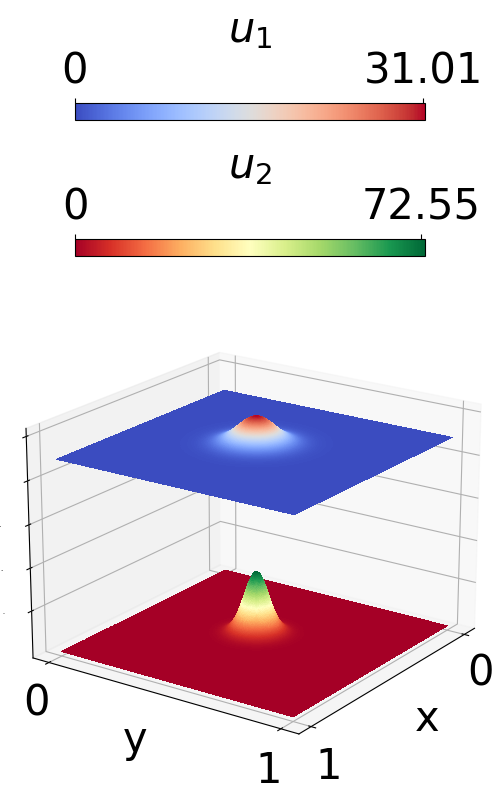
(a) $R_{2}=0.3$

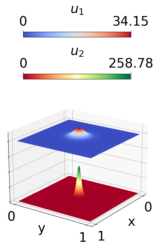
(b) $R_{2}=0.2$

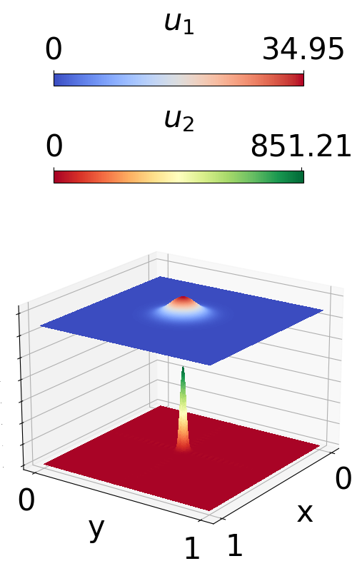
(c) $R_{2}=0.1$

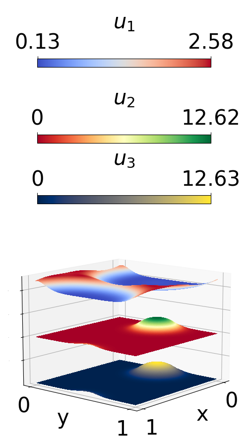
(d) $R_{3}=0.3$

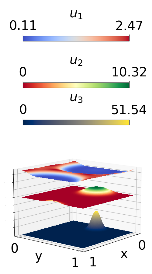
(e) $R_{3}=0.2$

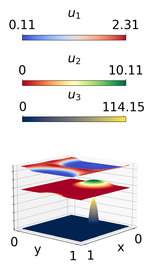
(f) $R_{3}=0.1$

Figure 1: Numerical simulations of Equations (1) on square domains with $N=2$ in (a)-(b), and $N=3$ in (d)-(f), for decreasing values of the sensig range $R_{i}$ of the population $u_{i}$. In (a)-(b): $D_{1}=D_{2}=1$, $\gamma_{11}=\gamma_{22}=0$, $\gamma_{12}=\gamma_{21}=-1.2$, $R_{1}=0.4$. In (d)-(f): $D_{1}=D_{2}=D_{3}=1$, $\gamma_{11}=\gamma_{12}=\gamma_{13}=1$, $\gamma_{21}=-\gamma_{22}=-\gamma_{23}=1$, $\gamma_{31}=-\gamma_{32}=-\gamma_{33}=1$, $R_{1}=0.4$, $R_{2}=0.3$.

Acknowledgements: JRP and VG acknowledge support of Engineering and Physical Sciences Research Council (EPSRC) grant EP/V002988/1 awarded to JRP. VG is also grateful for support from the National Group of Mathematical Physics (GNFM-INdAM). TH is supported through a discovery grant of the Natural Science and Engineering Research Council of Canada (NSERC), RGPIN-2017-04158. MAL gratefully acknowledges support from NSERC Discovery Grant RGPIN-2018-05210 and from the Gilbert and Betty Kennedy Chair in Mathematical Biology.

References

• [1] R. C. Fetecau, Y. Huang, T. Kolokolnikov, Swarm dynamics and equilibria for a nonlocal aggregation model, Nonlinearity 24 (10) (2011) 2681.
• [2] J. R. Potts, M. A. Lewis, Spatial memory and taxis-driven pattern formation in model ecosystems, Bulletin of mathematical biology 81 (7) (2019) 2725–2747.
• [3] K. Painter, J. Potts, T. Hillen, Biological modelling with nonlocal advection diffusion equations, Math. Models Methods in Appl. Sci. (M3AS) (2023).
• [4] J. Carrillo, R. Galvani, G. Pavliotis, A. Schlichting, Long-time behavior and phase transitions for the McKean-Vlasov equation on a torus, Archives Rational Mechanics and Analysis 235 (2020) 635–690.
• [5] A. Jüngel, S. Portisch, A. Zurek, Nonlocal cross-diffusion systems for multi-species populations and networks, Nonlinear Analysis 219 (2022) 112800.
• [6] V. Giunta, T. Hillen, M. Lewis, J. R. Potts, Local and global existence for nonlocal multispecies advection-diffusion models, SIAM Journal on Applied Dynamical Systems 21 (3) (2022) 1686–1708.
• [7] T. Hillen, K. Painter, Global existence for a parabolic chemotaxis model with prevention of overcrowding, Adv. Appl. Math. 26 (2001) 280–301.
• [8] L. C. Evans, Partial differential equations, Vol. 19, American Mathematical Society, 2022.
• [9] D. Horstmann, From 1970 until present: The Keller-Segel model in chemotaxis and its consequences I, Jahresberichte der DMV 105 (3) (2003) 103–165.
• [10] T. Hillen, K. Painter, A user’s guide to PDE models for chemotaxis, J. Math. Biol. 58 (2009) 183–217.
• [11] B. Perthame, Transport Equations in Biology, Birkhäuser, 2007.