CTPU-PTC-23-47, UT-Komaba/23-13

Analytic Formulae for Inflationary Correlators with Dynamical Mass

Shuntaro Aoki ¹, Toshifumi Noumi ², Fumiya Sano ^3,4,

Masahide Yamaguchi ^4,3

¹Particle Theory and Cosmology Group, Center for Theoretical Physics of the Universe,
Institute for Basic Science, Daejeon, 34126, Korea

²Graduate School of Arts and Sciences, The University of Tokyo, Tokyo 153-8902, Japan

³Department of Physics, Tokyo Institute of Technology, Tokyo 152-8551, Japan

⁴Cosmology, Gravity and Astroparticle Physics Group, Center for Theoretical Physics of the Universe, Institute for Basic Science, Daejeon 34126, Korea

Abstract
Massive fields can imprint unique oscillatory features on primordial correlation functions or inflationary correlators, which is dubbed the cosmological collider signal. In this work, we analytically investigate the effects of a time-dependent mass of a scalar field on inflationary correlators, extending previous numerical studies and implementing techniques developed in the cosmological bootstrap program. The time-dependent mass is in general induced by couplings to the slow-roll inflaton background, with particularly significant effects in the case of non-derivative couplings. By linearly approximating the time dependence, the mode function of the massive scalar is computed analytically, on which we derive analytic formulae for two-, three-, and four-point correlators with the tree-level exchange of the massive scalar. The obtained formulae are utilized to discuss the phenomenological impacts on the power spectrum and bispectrum, and it is found that the scaling behavior of the bispectrum in the squeezed configuration, i.e., the cosmological collider signal, is modified from a time-dependent Boltzmann suppression. By investigating the scaling behavior in detail, we are in principle able to determine the non-derivative couplings between the inflaton and the massive particle.

 

diagram

1 Introduction

Observations of the Cosmic Microwave Background [1, 2, 3] strongly support the existence of cosmic inflation [4, 5, 6, 7, 8] which can give solutions to several problems in the standard cosmology as well as is the source of primordial scalar (curvature) and tensor perturbations. Furthermore, given the high energy scale ($\rho^{1/4}_{\text{inf}}\sim 10^{15}$ GeV at most), inflation is a unique opportunity to explore high energy physics including models beyond the Standard Model.

In recent year, there has been a growing interest in an approach that exploit higher-point correlation functions, or non-Gaussianity, of scalar and tensor perturbations, called cosmological collider (CC) program (see earlier works [9, 10, 11, 12] and recent developments [13, 14, 15, 16, 17, 18, 19, 20, 21, 22, 23, 24, 25, 26, 27, 28, 29, 30, 31, 32, 33, 34, 33, 35, 36, 37, 38, 39, 40, 41, 42, 43, 42, 38, 44, 45, 46, 47, 48, 49, 50, 51, 52, 53, 54, 55, 56, 57, 58, 59, 60, 61, 62, 63, 64, 65, 66, 67, 68, 69, 70, 70, 71, 72, 73, 74, 75, 76, 77, 78, 79, 80, 81, 82, 83, 84, 85, 86, 87, 88, 89, 90, 91, 92, 93, 94, 95, 96, 97, 98, 99, 100]). Indeed, these correlation functions can contain information of (possibly new) massive particles created during inflation, and especially in the soft limits, we expect a sharp oscillatory behavior (what we call “signal”) characterized by the mass of particles around the Hubble scale.

A number of recent developments have been seen in the computational methods of primordial correlators. In particular, the so-called cosmological bootstrap method [101, 102, 103, 104, 105, 106, 107, 108, 109, 110, 111, 112, 113, 114, 115, 116, 117, 118, 119, 120, 121, 122, 123, 124, 125, 126, 127, 128, 129, 130, 131, 132, 133, 134, 135, 136, 137] (see also AdS techniques [138, 139, 140, 141, 142, 143]) has made it possible to compute the correlation functions rigorously and analytically without having to perform the awkward time integrals of special functions in the cosmological in-in calculations (see Ref. [144, 145] for the detail). This allows us to evaluate not only the signal parts of CC but also the non-oscillatory parts (background). This is quite important to understand how large the net signal is.

So far, most of the studies have focused on situations where the masses of massive fields are constant, and consequently, the correlation function has a scale-invariant form. However, interactions with inflaton can produce a non-negligible time dependence on the masses of these massive fields, resulting in a scale-dependent correlation function. For example in Ref. [86], it is numerically shown that a significant deviation from the standard CC signal in bispectrum can be obtained in case of the non-derivative coupling $e^{\alpha\phi/M_{\text{Pl}}}\sigma^{2}$, where $\phi$ is an inflaton and $\sigma$ is an isocurvaton.

In this paper, we derive analytic formulae for two-, three-, and four-point inflaton correlation functions or “inflationary correlators”. We focus on a simple model consisting of an inflaton and a massive scalar field, where the inflaton imparts a time dependence on the massive scalar through interactions. We then solve the so-called “bootstrap equations” for the correlators [101] by approximating the time-dependence of the mass at the linear order of time. In the constant mass limit, our results consistently reproduce those obtained in Refs. [128, 132]. The analytic formulae allow us to take into account arbitrary momentum configurations and background parts, so that we can extract various phenomenological aspects of non-Gaussianity in a more precise manner. Specifically, the bispectrum (three-point correlation function of the curvature perturbation) in the squeezed limit contains information on the time dependence of the mass of $\sigma$, which is useful to distinguish couplings between inflaton and the massive field.

The paper is organized as follows. In section 2, we introduce the above setup and solve the mode equations for a massive scalar field with time-dependent mass. We also introduce integral formulae for the two-, three-, and four-point correlators of interest. We then derive and solve the bootstrap equations satisfied by the correlators in section 3. In section 4, we discuss the observational impact by taking a particular interaction between the inflaton and the massive scalar. Section 5 is devoted to the summary. Appendices A and B provide boundary conditions necessary to solve the bootstrap equations, and a consistency check in the constant mass limit.

Notations

The spacetime metric is Friedman–Lemaître–Robertson–Walker (FLRW) metric: $\mathrm{d}s^{2}=-\mathrm{d}t^{2}+a^{2}(t)\mathrm{d}\mathbf{x}^{2}=a^{2}(\tau)(-\mathrm{d}\tau^{2}+\mathrm{d}\mathbf{x}^{2})$, where $t$ and $\tau$ are physical time and conformal time respectively. In (quasi) de Sitter space, a scale factor is given by $a(\tau)=-1/H\tau$ with the Hubble parameter $H$. Regarding the derivative with respect to physical time (conformal time), we use a dot (prime) for operation, i.e., $\cdot=\mathrm{d}/\mathrm{d}t$ and $\prime=\mathrm{d}/\mathrm{d}\tau$.

2 Setup

In this work, we consider a simple system consisting of only an inflaton $\phi$ and a massive scalar $\sigma$, and assume that their interactions include the following non-derivative coupling:

$$\mathcal{L}_{\text{int}}\supset-\frac{1}{2}g(\phi)\sigma^{2}.$$ (2.1)

During inflation, the interaction (2.1) gives an effective mass of $\sigma$, $m_{\rm{eff}}^{2}=g(\phi_{0}(t))$ with $\phi_{0}(t)$ being the inflaton background, and thus the mass of $\sigma$ becomes time-dependent. We will first investigate the effects of time dependence with Eq. (2.1) on the mode function of $\sigma$. Then, based on the mode function derived there, we study its impact on the inflationary correlation functions in the next sections.

2.1 Mode functions and propagators with time-dependent mass

Canonical quantization

We quantize the inflaton fluctuation $\delta\phi$ and the massive scalar $\sigma$ with the mode expansion

$$\delta\phi(\tau,\mathbf{x}) =\int\frac{\mathrm{d}^{3}\mathbf{k}}{(2\pi)^{3}}\left(u_{k}(\tau)a_{\mathbf{k}}+u_{k}^{*}(\tau)a_{-\mathbf{k}}^{\dagger}\right)e^{\mathrm{i}{\mathbf{k}\cdot\mathbf{x}}},$$ (2.2)

$$\sigma(\tau,\mathbf{x}) =\int\frac{\mathrm{d}^{3}\mathbf{k}}{(2\pi)^{3}}\left(v_{k}(\tau)b_{\mathbf{k}}+v_{k}^{*}(\tau)b_{-\mathbf{k}}^{\dagger}\right)e^{\mathrm{i}{\mathbf{k}\cdot\mathbf{x}}},$$ (2.3)

and the commutation relations for the annihilation and the creation operators

$$[a_{\mathbf{k}},a^{\dagger}_{\mathbf{k}^{\prime}}]=(2\pi)^{3}\delta^{3}({\mathbf{k}}-{\mathbf{k}^{\prime}}),\quad[b_{\mathbf{k}},b^{\dagger}_{\mathbf{k}^{\prime}}]=(2\pi)^{3}\delta^{3}({\mathbf{k}}-{\mathbf{k}^{\prime}}).$$ (2.4)

Note that $\mathbf{k}$ expresses three-dimensional vectors, and $k\equiv\left|\mathbf{k}\right|$ is the absolute value. Under the slow-roll approximation, the mode function of inflaton fluctuations, $u_{k}$, satisfies an equation of motion for a massless scalar field in de Sitter spacetime,

$$u_{k}^{\prime\prime}-\frac{2}{\tau}u_{k}^{\prime}+k^{2}u_{k}=0.$$ (2.5)

Assuming the Bunch–Davies vacuum, we obtain the canonically normalized mode function

$$u_{k}=\frac{H}{\sqrt{2k^{3}}}(1+\mathrm{i}k\tau)e^{-\mathrm{i}k\tau}.$$ (2.6)

On the other hand, the mode function of the massive field, $v_{k}$, satisfies the following equation:

$$v_{k}^{\prime\prime}-\frac{2}{\tau}v_{k}^{\prime}+\left(k^{2}+\frac{m^{2}_{\rm{eff}}}{H^{2}\tau^{2}}\right)v_{k}=0.$$ (2.7)

Here $m^{2}_{\rm{eff}}\equiv g(\phi_{0}(t))$ is an effective mass of $\sigma$, which in general depends on time.

Approximation of effective mass for analytic computations

In the forthcoming analysis, we impose several assumptions on the effective mass $m_{\rm eff}$ and employ approximations to perform analytic computations. To explain them, we begin by recalling that, within the framework of the slow-roll approximation, the inflaton background is described by

$$\phi_{0}(\tau)=\sqrt{2\epsilon}M_{\text{Pl}}\log\left(\frac{\tau}{\tau_{0}}\right),$$ (2.8)

where we used $\phi_{0}^{\prime}=\sqrt{2\epsilon}M_{\text{Pl}}/\tau$ (assuming $\dot{\phi}_{0}<0$ without loss of generality) and introduced a reference time $\tau_{0}$ as an integration constant. In this context, the value of the background inflaton field $\phi_{0*}$ at the horizon crossing time $\tau_{*}$ for a mode $k$ is given by

$$\phi_{0*}=\sqrt{2\epsilon}M_{\text{Pl}}\log\left(\frac{\tau_{*}}{\tau_{0}}\right)=-\sqrt{2\epsilon}M_{\text{Pl}}\log v(k),\quad v(k)\equiv\frac{k}{k_{0}},$$ (2.9)

where we used the condition $k\tau_{*}=-1$ and also introduced a reference scale $k_{0}$ such that $k_{0}\tau_{0}=-1$. The effective mass at the horizon crossing of the mode $k$ reads

$$m_{\rm eff}^{2}(\tau_{*})=g(\phi_{0*})\equiv g_{*}(v).$$ (2.10)

We are interested in the situation where the variation of the effective mass is not negligible, i.e., $|\Delta m_{\rm eff}^{2}|\gtrsim m_{\rm eff}^{2}$ during observable inflation with e-folding number roughly $50\lesssim N\lesssim 60$ for CMB, where $\Delta m_{\rm eff}^{2}$ represents the change in the square of the effective mass from the beginning to the end of observable inflation. It is worth emphasizing that, under this condition, the time dependence of the effective mass produces significant effects that dominate over other slow-roll suppressed effects such as the inflaton mass. Moreover, we mainly focus on the situation that the effective mass remains at the Hubble scale throughout inflation, $m_{\rm eff}\sim H$, and undergoes several times larger or smaller changes relative to the initial mass. This assumption is made to avoid exponential suppression of the CC signal $\sim e^{-\mathcal{O}(m_{\rm eff}/H)}$.

When we solve the equation of motion (2.7) for the massive field $\sigma$, it is also necessary to consider the time evolution of the effective mass around the time of the horizon crossing. In order to estimate the effect, let us perform an expansion of the inflaton background $\phi_{0}(\tau)$ around the horizon crossing time $\tau_{*}$ as

$$\phi_{0}(\tau)=\phi_{0*}-\sqrt{2\epsilon}M_{\text{Pl}}\left(1-\frac{\tau}{\tau_{*}}\right)+\cdots,$$ (2.11)

where the dots stand for higher order terms in $1-(\tau/\tau_{*})$. Correspondingly, we expand the effective mass as

$$m^{2}_{\rm{eff}}(\tau)=g_{*}-g_{\phi,*}\sqrt{2\epsilon}M_{\text{Pl}}\left(1-\frac{\tau}{\tau_{*}}\right)+\cdots,$$ (2.12)

where $g_{\phi,*}\equiv\mathrm{d}g/\mathrm{d}\phi|_{\phi=\phi_{0*}}$. The expansion works well at least within a span of several e-foldings around the horizon crossing if the following condition is satisfied:

$$\frac{|g_{\phi,*}|M_{\text{Pl}}}{g_{*}}\lesssim\epsilon^{-1/2}.$$ (2.13)

In the following analysis, we will take into account the leading order correction, specifically, the second term of Eq. (2.12). On the other hand, the previously mentioned condition $|\Delta m_{\rm eff}^{2}|\gtrsim m_{\rm eff}^{2}$ for non-negligible time dependence during inflation can be rephrased as $|g_{\phi,*}|M_{\text{Pl}}/g_{*}\gtrsim\epsilon^{-1/2}N^{-1}$ with $N$ being the e-folding number of observable inflation and $m_{\rm eff}^{2}$ being evaluated at the horizon crossing time. To sum up, there exists a parameter regime where both conditions are simultaneously satisfied:

$$\epsilon^{-1/2}N^{-1}\lesssim\frac{|g_{\phi,*}|M_{\text{Pl}}}{g_{*}}\lesssim\epsilon^{-1/2}.$$ (2.14)

We work in this regime and study the effects of the time-dependent mass analytically.

Analytical mode function for massive field

With the leading order correction in Eq. (2.12), we simplify the equation of motion (2.7) for the massive field $\sigma$ to

$$v_{k}^{\prime\prime}-\frac{2}{\tau}v_{k}^{\prime}+\left(k^{2}+\frac{\mu^{2}+9/4}{\tau^{2}}+\frac{2k\kappa}{\tau}\right)v_{k}=0$$ (2.15)

where

$$\mu^{2}\equiv\frac{g_{*}}{H^{2}}\left(1-\frac{\sqrt{2\epsilon}g_{\phi,*}M_{\text{Pl}}}{g_{*}}\right)-\frac{9}{4},\quad\kappa\equiv-\frac{g_{*}}{2H^{2}}\frac{\sqrt{2\epsilon}g_{\phi,*}M_{\text{Pl}}}{g_{*}}.$$ (2.16)

It is important to note that $g_{*}$ and $g_{\phi,*}$ are functions of $v(k)=k/k_{0}$, thus $\mu$ and $\kappa$ have scale dependence accordingly. We can solve Eq. (2.15) analytically as

$$v_{k}=\frac{e^{\pi\kappa/2}}{\sqrt{2k}}H(-\tau)W_{-\mathrm{i}\kappa,\mathrm{i}\mu}(2\mathrm{i}k\tau),$$ (2.17)

where $W_{a,b}(\cdot)$ is the Whittaker function. Note that when the mass of $\sigma$ is constant, $g(\phi)=m_{0}^{2}$ (and hence $\kappa=0$), Eq. (2.17) is reduced to

$$v_{k}=e^{-\frac{\pi}{2}\mu+\mathrm{i}\frac{\pi}{4}}\frac{\sqrt{\pi}}{2}H(-\tau)^{3/2}H_{\mathrm{i}\mu}^{(1)}(-k\tau)$$ (2.18)

with $\mu=\sqrt{(m_{0}/H)^{2}-9/4}$, which reproduces the of mode function for a constant mass [9].

Propagators

Based on the mode functions, (2.6) and (2.17), one can construct Schwinger–Keldysh (SK) propagators as follows (see Ref. [145] for details).

• Bulk-to-boundary propagators for the inflaton fluctuation $\delta\phi$:

  $$G_{\mathrm{a}}(k;\tau)=\frac{H^{2}}{2k^{3}}(1-\mathrm{i}\mathrm{a}k\tau)e^{\mathrm{i}\mathrm{a}k\tau},$$ (2.19)

  where ${\mathrm{a}}=\pm$.

• Bulk-to-bulk propagators $D_{\mathrm{ab}}$ with ${\mathrm{a},\mathrm{b}}=\pm$ for the massive field $\sigma$:

  $$D_{\pm\mp}\left(k;\tau_{1},\tau_{2}\right)=D_{\lessgtr}\left(k;\tau_{1},\tau_{2}\right),$$ (2.20)

  $$D_{\pm\pm}\left(k;\tau_{1},\tau_{2}\right)=D_{\gtrless}\left(k;\tau_{1},\tau_{2}\right)\theta\left(\tau_{1}-\tau_{2}\right)+D_{\lessgtr}\left(k;\tau_{1},\tau_{2}\right)\theta\left(\tau_{2}-\tau_{1}\right),$$ (2.21)

  where $\theta(\cdot)$ is a unit step function and

  $$D_{>}\left(k;\tau_{1},\tau_{2}\right)=v_{k}\left(\tau_{1}\right)v_{k}^{*}\left(\tau_{2}\right)=\frac{e^{\pi\kappa}}{2k}H^{2}(\tau_{1}\tau_{2})W_{-\mathrm{i}\kappa,\mathrm{i}\mu}(2\mathrm{i}k\tau_{1})W_{\mathrm{i}\kappa,-\mathrm{i}\mu}(-2\mathrm{i}k\tau_{2}),$$ (2.22)

  $$D_{<}\left(k;\tau_{1},\tau_{2}\right)=D_{>}^{*}\left(k;\tau_{1},\tau_{2}\right).$$ (2.23)

2.2 Inflationary correlators

Here, we specify inflationary correlation functions to be investigated in this paper. The correlation functions can be computed from the formula [144],

$$\left\langle\mathcal{O}\right\rangle\equiv\langle 0|\left[\bar{\mathrm{T}}\exp\left(\mathrm{i}\int_{-\infty}^{0}\mathrm{d}\tau^{\prime}H_{I}\left(\tau^{\prime}\right)\right)\right]\mathcal{O}_{I}\left[\mathrm{T}\exp\left(-\mathrm{i}\int_{-\infty}^{0}\mathrm{d}\tau^{\prime}H_{I}\left(\tau^{\prime}\right)\right)\right]|0\rangle,$$ (2.24)

where $\mathcal{O}$ is the operator of our interest, and $\mathrm{T}\ (\bar{\mathrm{T}})$ is a (anti) time-ordering operator. $H_{I}$ is an interaction Hamiltonian, and all quantities on the right-hand side are understood in the interaction picture.

Interactions

In addition to Eq. (2.1), we assume the presence of the following derivative (shift-symmetric with respect to $\delta\phi$) interactions involving the inflaton fluctuation $\delta\phi$ and the massive scalar $\sigma$,

$$\mathcal{L}_{2,{\rm{int}}}=c_{2}(-H\tau)^{-3}\sigma\delta\phi^{\prime},$$ (2.25)

$$\mathcal{L}_{3,{\rm{int}}}=c_{3}(-H\tau)^{-2}\sigma(\delta\phi^{\prime})^{2},$$ (2.26)

where $c_{2}$ and $c_{3}$ are coupling constants with mass dimension $1$ and $-1$, respectively. With the presence of the interactions and the formula (2.24), we can calculate inflationary correlators $\left\langle\delta\phi\cdots\delta\phi\right\rangle$. In particular, this paper focuses on analyzing the two-, three-, and four-point correlation functions of the inflaton fluctuations as shown in Fig. 1.

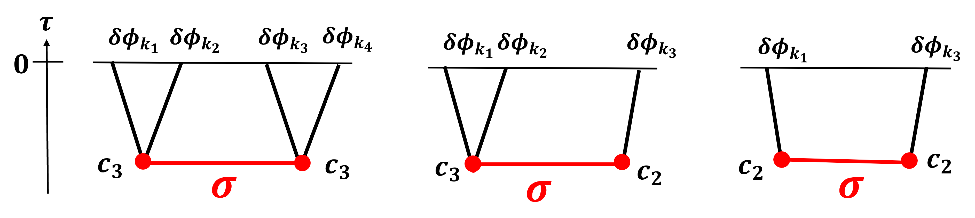
Figure 1: Diagrams with a massive scalar field $\sigma$ with time-dependent mass.

4-point correlators

Let us begin with the correction to the four-point correlation functions since its specific limit produces the three- and two-point correlation functions.

By employing the in-in formula (2.24) (or SK diagrammatic rule [145]), we obtain

$$\langle\delta\phi_{\bf{k}_{1}}\delta\phi_{\bf{k}_{2}}\delta\phi_{\bf{k}_{3}}\delta\phi_{\bf{k}_{4}}\rangle^{\prime}$$

$$=-4\frac{c_{3}^{2}}{H^{4}}\sum_{\mathrm{a},\mathrm{b}=\pm}\mathrm{ab}\int\frac{\mathrm{d}\tau_{1}}{\left(-\tau_{1}\right)^{2}}\frac{\mathrm{d}\tau_{2}}{\left(-\tau_{2}\right)^{2}}G^{\prime}_{\mathrm{a}}(k_{1};\tau_{1})G^{\prime}_{\mathrm{a}}(k_{2};\tau_{1})G^{\prime}_{\mathrm{b}}(k_{3};\tau_{2})G^{\prime}_{\mathrm{b}}(k_{4};\tau_{2})D_{\mathrm{ab}}\left(k_{s};\tau_{1},\tau_{2}\right)+{\rm{5per.}},$$ (2.27)

where the prime on the left-hand side means that a momentum conservation factor $(2\pi)^{3}\delta^{(3)}({\bf{k}}_{1}+\cdots+{\bf{k}}_{4})$ is extracted, and “5 per.” represents permutations of the external momenta ${\bf{k}}_{i}\ (i=1,\cdots,4)$. The propagators $G_{\mathrm{a}}$ and $D_{\mathrm{ab}}$ are given in Eqs. (2.19), (2.20) and (2.21) respectively, and $k_{s}\equiv|\mathbf{k}_{1}+\mathbf{k}_{2}|$ is the “$s$-channel” momentum. This can be further simplified as

$$\langle\delta\phi_{\bf{k}_{1}}\delta\phi_{\bf{k}_{2}}\delta\phi_{\bf{k}_{3}}\delta\phi_{\bf{k}_{4}}\rangle^{\prime}$$

$$=-4c_{3}^{2}H^{4}\cdot\frac{1}{16k_{1}k_{2}k_{3}k_{4}}\sum_{\mathrm{a},\mathrm{b}=\pm}\mathrm{ab}\int\mathrm{d}\tau_{1}\mathrm{d}\tau_{2}e^{\mathrm{i}\mathrm{a}k_{12}\tau_{1}+\mathrm{i}\mathrm{b}k_{34}\tau_{2}}D_{\mathrm{ab}}\left(k_{s};\tau_{1},\tau_{2}\right)+{\rm{5per.}}$$

$$=4c_{3}^{2}H^{4}\cdot\frac{1}{16k_{1}k_{2}k_{3}k_{4}k_{s}^{5}}\sum_{\mathrm{a},\mathrm{b}=\pm}\mathcal{I}_{\mathrm{ab}}^{0,0}+{\rm{5per.}},$$ (2.28)

where $k_{12}\equiv k_{1}+k_{2}$ and $k_{34}\equiv k_{3}+k_{4}$. In the first line we inserted the explicit expression of $G_{\mathrm{a}}$, and in the second line we introduced a “seed integral” [128, 132],

$$\mathcal{I}_{\mathrm{ab}}^{p_{1}p_{2}}\equiv-\mathrm{ab}k_{s}^{5+p_{12}}\int_{-\infty}^{0}\mathrm{~{}d}\tau_{1}\mathrm{~{}d}\tau_{2}\left(-\tau_{1}\right)^{p_{1}}\left(-\tau_{2}\right)^{p_{2}}e^{\mathrm{i}\mathrm{a}k_{12}\tau_{1}+\mathrm{i}\mathrm{b}k_{34}\tau_{2}}D_{\mathrm{ab}}\left(k_{s};\tau_{1},\tau_{2}\right),$$ (2.29)

with $p_{1}$ and $p_{2}$ being constant numbers with $p_{1,2}>-5/2$, and $p_{12}\equiv p_{1}+p_{2}$. Therefore, once the seed integral (2.29) is computed, the four-point correlation function can be automatically obtained from Eq. (2.28), and this is also true for three- and two-point functions, as shown below.

3-point correlators

In the same way, by utilizing the seed integral (2.29), the three-point function is given by

$$\langle\delta\phi_{\bf{k}_{1}}\delta\phi_{\bf{k}_{2}}\delta\phi_{\bf{k}_{3}}\rangle^{\prime}$$

$$=-2\frac{c_{2}c_{3}}{H^{5}}\sum_{\mathrm{a},\mathrm{b}=\pm}\mathrm{ab}\int\frac{\mathrm{d}\tau_{1}}{\left(-\tau_{1}\right)^{2}}\frac{\mathrm{d}\tau_{2}}{\left(-\tau_{2}\right)^{3}}G^{\prime}_{\mathrm{a}}(k_{1};\tau_{1})G^{\prime}_{\mathrm{a}}(k_{2};\tau_{1})G^{\prime}_{\mathrm{b}}(k_{3};\tau_{2})D_{\mathrm{ab}}\left(k_{3};\tau_{1},\tau_{2}\right)+{\rm{2per.}}$$

$$=2c_{2}c_{3}H\cdot\frac{1}{8k_{1}k_{2}k_{3}}\sum_{\mathrm{a},\mathrm{b}=\pm}\mathrm{ab}\int\mathrm{d}\tau_{1}\frac{\mathrm{d}\tau_{2}}{\left(-\tau_{2}\right)^{2}}e^{\mathrm{i}\mathrm{a}k_{12}\tau_{1}+\mathrm{i}\mathrm{b}k_{3}\tau_{2}}D_{\mathrm{ab}}\left(k_{3};\tau_{1},\tau_{2}\right)+{\rm{2per.}}$$

$$=-2c_{2}c_{3}H\cdot\frac{1}{8k_{1}k_{2}k_{3}^{4}}\lim_{k_{4}\to 0}\sum_{\mathrm{a},\mathrm{b}=\pm}\mathcal{I}_{\mathrm{ab}}^{0,-2}+{\rm{2per.}}.$$ (2.30)

The three-point correlator corresponds to a soft limit ($k_{4}\rightarrow 0$) of the four-point one or the seed integral.

2-point correlators

Finally, the leading order correction to the two-point function is described as follows:

$$\langle\delta\phi_{\bf{k}_{1}}\delta\phi_{\bf{k}_{3}}\rangle^{\prime} =-2\frac{c_{2}^{2}}{H^{6}}\sum_{\mathrm{a},\mathrm{b}=\pm}\mathrm{ab}\int\frac{\mathrm{d}\tau_{1}}{\left(-\tau_{1}\right)^{3}}\frac{\mathrm{d}\tau_{2}}{\left(-\tau_{2}\right)^{3}}G^{\prime}_{\mathrm{a}}(k_{1};\tau_{1})G^{\prime}_{\mathrm{b}}(k_{1};\tau_{2})D_{\mathrm{ab}}\left(k_{1};\tau_{1},\tau_{2}\right)$$

$$=-2\frac{c_{2}^{2}}{H^{2}}\cdot\frac{1}{4k_{1}^{2}}\sum_{\mathrm{a},\mathrm{b}=\pm}\mathrm{ab}\int\frac{\mathrm{d}\tau_{1}}{\left(-\tau_{1}\right)^{2}}\frac{\mathrm{d}\tau_{2}}{\left(-\tau_{2}\right)^{2}}e^{\mathrm{i}\mathrm{a}k_{1}\tau_{1}+\mathrm{i}\mathrm{b}k_{1}\tau_{2}}D_{\mathrm{ab}}\left(k_{1};\tau_{1},\tau_{2}\right)$$

$$=2\frac{c_{2}^{2}}{H^{2}}\cdot\frac{1}{4k_{1}^{3}}\lim_{k_{2},k_{4}\to 0}\sum_{\mathrm{a},\mathrm{b}=\pm}\mathcal{I}_{\mathrm{ab}}^{-2,-2}.$$ (2.31)

Here, we need an expression for double soft limits ($k_{2},k_{4}\rightarrow 0$) of the seed integral. Note that the above correlator is a correction to the one in free theory, $\langle\delta\phi_{\bf{k}_{1}}\delta\phi_{\bf{k}_{3}}\rangle^{\prime}=H^{2}/2k_{1}^{3}$.

3 Bootstrapping Seed Integrals with Time-dependent Mass

Our task is reduced to evaluate the seed integral (2.29),

$$\mathcal{I}_{\mathrm{ab}}^{p_{1}p_{2}}\equiv-\mathrm{ab}k_{s}^{5+p_{12}}\int_{-\infty}^{0}\mathrm{~{}d}\tau_{1}\mathrm{~{}d}\tau_{2}\left(-\tau_{1}\right)^{p_{1}}\left(-\tau_{2}\right)^{p_{2}}e^{\mathrm{i}\mathrm{a}k_{12}\tau_{1}+\mathrm{i}\mathrm{b}k_{34}\tau_{2}}D_{\mathrm{ab}}\left(k_{s};\tau_{1},\tau_{2}\right).$$ (3.1)

Performing the time-integral in Eq. (3.1) is challenging for general momentum configurations. Therefore, we employ another approach developed in Refs. [101, 128, 132], where we can obtain analytic expressions for the seed integrals by solving differential equations (“bootstrap equations”) for Eq. (3.1). We will see that this method is also applicable to our case. Note that this section describes technical details, so readers who are not interested in the derivation can skip to the final results, Eqs. (3.77), (3.89) for the seed integral, Eqs. (3.103), (3.112) for its single soft limit, and Eqs. (3.127), (3.135) for the double soft limit.

3.1 Bootstrap equations

The SK propagators in Eqs. (2.20) and (2.21) satisfy the following differential equations

$$\left(\tau_{1}^{2}\partial_{\tau_{1}}^{2}-2\tau_{1}\partial_{\tau_{1}}+k_{s}^{2}\tau_{1}^{2}+\mu^{2}+\frac{9}{4}+2\kappa k_{s}\tau_{1}\right)D_{\pm\mp}\left(k_{s};\tau_{1},\tau_{2}\right)=0,$$ (3.2)

$$\left(\tau_{1}^{2}\partial_{\tau_{1}}^{2}-2\tau_{1}\partial_{\tau_{1}}+k_{s}^{2}\tau_{1}^{2}+\mu^{2}+\frac{9}{4}+2\kappa k_{s}\tau_{1}\right)D_{\pm\pm}\left(k_{s};\tau_{1},\tau_{2}\right)=\mp\mathrm{i}H^{2}\tau_{1}^{2}\tau_{2}^{2}\delta\left(\tau_{1}-\tau_{2}\right),$$ (3.3)

where we recall $k_{s}\equiv|\mathbf{k}_{1}+\mathbf{k}_{2}|$. They satisfy the same differential equations with respect to $\tau_{2}$. By introducing

$$z_{1}=-k_{12}\tau_{1},\quad z_{2}=-k_{34}\tau_{2},$$ (3.4)

with $k_{12}\equiv k_{1}+k_{2}$ and $k_{34}\equiv k_{3}+k_{4}$, and

$$r_{1}\equiv\frac{k_{s}}{k_{12}},\quad r_{2}\equiv\frac{k_{s}}{k_{34}},$$ (3.5)

Eqs. (3.2) and (3.3) can be rewritten as

$$\left(z_{1}^{2}\partial_{z_{1}}^{2}-2z_{1}\partial_{z_{1}}+r_{1}^{2}z_{1}^{2}+\mu^{2}+\frac{9}{4}-2\kappa r_{1}z_{1}\right)\widehat{D}_{\pm\mp}\left(r_{1}z_{1},r_{2}z_{2}\right)=0,$$ (3.6)

$$\left(z_{1}^{2}\partial_{z_{1}}^{2}-2z_{1}\partial_{z_{1}}+r_{1}^{2}z_{1}^{2}+\mu^{2}+\frac{9}{4}-2\kappa r_{1}z_{1}\right)\widehat{D}_{\pm\pm}\left(r_{1}z_{1},r_{2}z_{2}\right)=\mp\mathrm{i}H^{2}r_{1}^{2}z_{1}^{2}r_{2}^{2}z_{2}^{2}\delta\left(r_{1}z_{1}-r_{2}z_{2}\right),$$ (3.7)

where we defined $\widehat{D}_{\mathrm{ab}}=k_{s}^{3}D_{\mathrm{ab}}$, or explicitly,

$$\widehat{D}_{\pm\mp}\left(r_{1}z_{1},r_{2}z_{2}\right)=\frac{e^{\pi\kappa}}{2}H^{2}r_{1}z_{1}r_{2}z_{2}W_{\pm\mathrm{i}\kappa,\mp\mathrm{i}\mu}(\pm 2\mathrm{i}r_{1}z_{1})W_{\mp\mathrm{i}\kappa,\pm\mathrm{i}\mu}(\mp 2\mathrm{i}r_{2}z_{2}),$$ (3.8)

$$\widehat{D}_{\pm\pm}\left(r_{1}z_{1},r_{2}z_{2}\right)=\theta(r_{2}z_{2}-r_{1}z_{1})\widehat{D}_{\mp\pm}\left(r_{1}z_{1},r_{2}z_{2}\right)+\theta(r_{1}z_{1}-r_{2}z_{2})\widehat{D}_{\pm\mp}\left(r_{1}z_{1},r_{2}z_{2}\right).$$ (3.9)

An important observation is that $\widehat{D}$ depends on $z_{i}\ (i=1,2)$ with a specific combination $r_{i}z_{i}$. Thus, Eqs. (3.6) and (3.7) can be regarded as the differential equations with respect to $r_{i}$, i.e.,

$$\left(r_{1}^{2}\partial_{r_{1}}^{2}-2r_{1}\partial_{r_{1}}+r_{1}^{2}z_{1}^{2}+\mu^{2}+\frac{9}{4}-2\kappa r_{1}z_{1}\right)\widehat{D}_{\pm\mp}\left(r_{1}z_{1},r_{2}z_{2}\right)=0,$$ (3.10)

$$\left(r_{1}^{2}\partial_{r_{1}}^{2}-2r_{1}\partial_{r_{1}}+r_{1}^{2}z_{1}^{2}+\mu^{2}+\frac{9}{4}-2\kappa r_{1}z_{1}\right)\widehat{D}_{\pm\pm}\left(r_{1}z_{1},r_{2}z_{2}\right)=\mp\mathrm{i}H^{2}r_{1}^{2}z_{1}^{2}r_{2}^{2}z_{2}^{2}\delta\left(r_{1}z_{1}-r_{2}z_{2}\right),$$ (3.11)

and similarly for $r_{2}$.

The subsequent task is identifying differential equations (bootstrap equations) for the seed integral. In terms of $z_{i}$ and $r_{i}$, Eq. (3.1) is expressed as

$$\mathcal{I}_{\mathrm{ab}}^{p_{1}p_{2}}=(-\mathrm{ab})r_{1}^{1+p_{1}}r_{2}^{1+p_{2}}\int_{0}^{\infty}\mathrm{d}z_{1}\mathrm{~{}d}z_{2}z_{1}^{p_{1}}z_{2}^{p_{2}}e^{-\mathrm{ia}z_{1}-\mathrm{ib}z_{2}}\widehat{D}_{\mathrm{ab}}\left(r_{1}z_{1},r_{2}z_{2}\right).$$ (3.12)

Let us start from the opposite sign seed integral $\mathcal{I}_{\pm\mp}^{p_{1}p_{2}}$. By applying Eq. (3.10), $r_{1}^{-1-p_{1}}r_{2}^{-1-p_{2}}\mathcal{I}_{\pm\mp}^{p_{1}p_{2}}$ satisfies

$$\left(r_{1}^{2}\partial_{r_{1}}^{2}-2r_{1}\partial_{r_{1}}+\mu^{2}+\frac{9}{4}\right)\left(r_{1}^{-1-p_{1}}r_{2}^{-1-p_{2}}\mathcal{I}_{\pm\mp}^{p_{1}p_{2}}\right)$$

$$=\int_{0}^{\infty}\mathrm{d}z_{1}\mathrm{~{}d}z_{2}z_{1}^{p_{1}}z_{2}^{p_{2}}e^{\mp\mathrm{i}z_{1}\pm\mathrm{i}z_{2}}\left(r_{1}^{2}\partial_{r_{1}}^{2}-2r_{1}\partial_{r_{1}}+\mu^{2}+\frac{9}{4}\right)\widehat{D}_{\pm\mp}\left(r_{1}z_{1},r_{2}z_{2}\right)$$

$$=\int_{0}^{\infty}\mathrm{d}z_{1}\mathrm{~{}d}z_{2}z_{1}^{p_{1}}z_{2}^{p_{2}}e^{\mp\mathrm{i}z_{1}\pm\mathrm{i}z_{2}}\left(-r_{1}^{2}z_{1}^{2}+2\kappa r_{1}z_{1}\right)\widehat{D}_{\pm\mp}\left(r_{1}z_{1},r_{2}z_{2}\right)$$

$$=\left[r_{1}^{2}\left(r_{1}\partial_{r_{1}}+p_{1}+2\right)\left(r_{1}\partial_{r_{1}}+p_{1}+1\right)\mp 2\mathrm{i}\kappa r_{1}\left(r_{1}\partial_{r_{1}}+p_{1}+1\right)\right]\left(r_{1}^{-1-p_{1}}r_{2}^{-1-p_{2}}\mathcal{I}_{\pm\mp}^{p_{1}p_{2}}\right),$$ (3.13)

where we used the following formulae for an arbitrary function $f(rz)$,

$$\int_{0}^{\infty}dzz^{p+1}e^{-\mathrm{i}\mathrm{a}z}f(rz)=-\mathrm{i}\mathrm{a}(r\partial_{r}+p+1)\int_{0}^{\infty}z^{p}e^{-\mathrm{i}\mathrm{a}z}f(rz),$$ (3.14)

$$\int_{0}^{\infty}dzz^{p+2}e^{-\mathrm{i}\mathrm{a}z}f(rz)=-\left(r\partial_{r}+p+2\right)\left(r\partial_{r}+p+1\right)\int_{0}^{\infty}z^{p}e^{-\mathrm{i}\mathrm{a}z}f(rz),$$ (3.15)

from the third to the fourth line. Thus, we find

$$\left[\left(r_{1}^{2}-r_{1}^{4}\right)\partial_{r_{1}}^{2}-2\left(r_{1}+\left(p_{1}+2\right)r_{1}^{3}\mp\mathrm{i}\kappa r_{1}^{2}\right)\partial_{r_{1}}+\left(\mu^{2}+\frac{9}{4}-(p_{1}+1)(p_{1}+2)r_{1}^{2}\pm 2(p_{1}+1)\mathrm{i}\kappa r_{1}\right)\right]$$

$$\times\left(r_{1}^{-1-p_{1}}r_{2}^{-1-p_{2}}\mathcal{I}_{\pm\mp}^{p_{1}p_{2}}\right)=0,$$ (3.16)

or equivalently,

$$\mathcal{D}_{\pm,r_{1}}^{p_{1}}\mathcal{I}_{\pm\mp}^{p_{1}p_{2}}=0,$$ (3.17)

where

$$\mathcal{D}_{\pm,r}^{p}\equiv\left(r^{2}-r^{4}\right)\partial_{r}^{2}-2\left[(p+2)r+r^{3}\mp\mathrm{i}\kappa r^{2}\right]\partial_{r}+\mu^{2}+\frac{(5+2p)^{2}}{4}.$$ (3.18)

Eq. (3.17) gives the bootstrap equations for $\mathcal{I}_{\pm\mp}^{p_{1}p_{2}}$ with respect to $r_{1}$. Those with respect to $r_{2}$ are obtained in the same way, $\mathcal{D}_{\mp,r_{2}}^{p_{1}}\mathcal{I}_{\pm\mp}^{p_{1}p_{2}}=0$.

Let us shift our focus to the seed integral with the same sign, $\mathcal{I}_{\pm\pm}^{p_{1}p_{2}}$. The derivation is basically parallel to the previous case, except for the presence of the “source” term on the right-hand side of Eq. (3.7). In fact, we find

$$\left(r_{1}^{2}\partial_{r_{1}}^{2}-2r_{1}\partial_{r_{1}}+\mu^{2}+\frac{9}{4}\right)\left(r_{1}^{-1-p_{1}}r_{2}^{-1-p_{2}}\mathcal{I}_{\pm\pm}^{p_{1}p_{2}}\right)$$

$$=\left[r_{1}^{2}\left(r_{1}\partial_{r_{1}}+p_{1}+2\right)\left(r_{1}\partial_{r_{1}}+p_{1}+1\right)\mp 2\mathrm{i}\kappa r_{1}\left(r_{1}\partial_{r_{1}}+p_{1}+1\right)\right]\left(r_{1}^{-1-p_{1}}r_{2}^{-1-p_{2}}\mathcal{I}_{\pm\pm}^{p_{1}p_{2}}\right)$$

$$\ \ \ \ \pm\mathrm{i}H^{2}r_{1}^{2}r_{2}^{2}\int_{0}^{\infty}\mathrm{d}z_{1}\mathrm{~{}d}z_{2}z_{1}^{p_{1}+2}z_{2}^{p_{2}+2}e^{\mp\mathrm{i}z_{1}\mp\mathrm{i}z_{2}}\delta(r_{1}z_{1}-r_{2}z_{2}),$$ (3.19)

where the second term of the right-hand side is the new contribution. After performing the one-dimensional integral, we obtain the bootstrap equations

$$\mathcal{D}_{\pm,r_{1}}^{p_{1}}\mathcal{I}_{\pm\pm}^{p_{1}p_{2}}=H^{2}e^{\mp\mathrm{i}p_{12}\frac{\pi}{2}}\Gamma\left(5+p_{12}\right)\left(\frac{r_{1}r_{2}}{r_{1}+r_{2}}\right)^{5+p_{12}}.$$ (3.20)

The same equation for $r_{2}$ is provided with a replacement $\mathcal{D}_{\pm,r_{1}}^{p_{1}}\rightarrow\mathcal{D}_{\pm,r_{2}}^{p_{1}}$.

As pointed out in Refs. [128, 132], it is useful to introduce new variables

$$u_{i}\equiv\frac{2r_{i}}{1+r_{i}},\quad(i=1,2).$$ (3.21)

In terms of $u_{i}$, the set of bootstrap equations is summarized as

$$\mathcal{D}_{\pm,u_{1}}^{p_{1}}\mathcal{I}_{\pm\mp}^{p_{1}p_{2}}=0,$$ (3.22)

$$\mathcal{D}_{\pm,u_{1}}^{p_{1}}\mathcal{I}_{\pm\pm}^{p_{1}p_{2}}=H^{2}e^{\mp\mathrm{i}p_{12}\frac{\pi}{2}}\Gamma\left(5+p_{12}\right)\left(\frac{u_{1}u_{2}}{2\left(u_{1}+u_{2}-u_{1}u_{2}\right)}\right)^{5+p_{12}},$$ (3.23)

and

$$\mathcal{D}_{\mp,u_{2}}^{p_{2}}\mathcal{I}_{\pm\mp}^{p_{1}p_{2}}=0,$$ (3.24)

$$\mathcal{D}_{\pm,u_{2}}^{p_{2}}\mathcal{I}_{\pm\pm}^{p_{1}p_{2}}=H^{2}e^{\mp\mathrm{i}p_{12}\frac{\pi}{2}}\Gamma\left(5+p_{12}\right)\left(\frac{u_{1}u_{2}}{2\left(u_{1}+u_{2}-u_{1}u_{2}\right)}\right)^{5+p_{12}},$$ (3.25)

where

$$\mathcal{D}_{\pm,u}^{p}\equiv\left(u^{2}-u^{3}\right)\partial_{u}^{2}-\left[(4+2p)u-(1+p\pm\mathrm{i}\kappa)u^{2}\right]\partial_{u}+\left[\mu^{2}+\left(p+\frac{5}{2}\right)^{2}\right].$$ (3.26)

3.2 Solutions

Here we solve the bootstrap equations, (3.22), (3.23), (3.24), and (3.25).

Opposite sign seed $\mathcal{I}_{\pm\mp}^{p_{1}p_{2}}$

The opposite sign seeds $\mathcal{I}_{\pm\mp}^{p_{1}p_{2}}$ satisfy the homogeneous differential equations, (3.22) and (3.24). Considering each equation has two independent solutions, a general solution for $\mathcal{I}_{\pm\mp}^{p_{1}p_{2}}$ can be expressed as the following combination:

$$\mathcal{I}_{\pm\mp}^{p_{1}p_{2}}=\sum_{\mathrm{a},\mathrm{b}=\pm}\mathcal{C}_{\pm\mp\mid\mathrm{ab}}\ \mathcal{U}_{\pm\mid\mathrm{a}}^{p_{1}}\left(u_{1}\right)\mathcal{U}_{\mp\mid\mathrm{b}}^{p_{2}}\left(u_{2}\right),$$ (3.27)

where $\mathcal{C}_{\pm\mp\mid\mathrm{ab}}$ are coefficients fixed from boundary conditions later, and $\mathcal{U}_{\mathrm{a}\mid\mathrm{b}}(u)$ with $\mathrm{b}=\pm 1$ are the two independent solutions

$$\mathcal{U}_{\mathrm{a}\mid\mathrm{b}}^{p}(u)=\mathrm{iab}2^{\mathrm{iab}\mu}\pi\operatorname{csch}(2\pi\mu)\left(\frac{u}{2}\right)^{5/2+p+\mathrm{iab}\mu}{}_{2}\mathcal{F}_{1}\left[\begin{array}[]{c|c}\frac{5}{2}+p+\operatorname{iab}\mu,\frac{1}{2}-\mathrm{ia}\kappa+\operatorname{iab}\mu\\ 1+2\mathrm{iab}\mu\end{array}\ u\right].$$ (3.30)

Here, we inserted some numerical factors for later convenience, and ${}_{p}\mathcal{F}_{q}$ is defined by

$${}_{p}\mathcal{F}_{q}\left[\begin{array}[]{c|c}a_{1},\cdots,a_{p}\\ b_{1},\cdots,b_{q}\end{array}\ z\right]\equiv\Gamma\left[\begin{array}[]{c}a_{1},\cdots,a_{p}\\ b_{1},\cdots,b_{q}\end{array}\right]{}_{p}\mathrm{F}_{q}\left[\begin{array}[]{c|c}a_{1},\cdots,a_{p}\\ b_{1},\cdots,b_{q}\end{array}\ z\right],$$ (3.37)

where ${}_{p}\mathrm{F}_{q}$ is a generalized hypergeometric function, and the products of gamma function is abbreviated by

$$\Gamma\left[z_{1},\cdots,z_{m}\right]\equiv\Gamma\left(z_{1}\right)\cdots\Gamma\left(z_{m}\right),$$ (3.38)

$$\Gamma\left[\begin{array}[]{c}z_{1},\cdots,z_{m}\\ w_{1},\cdots,w_{n}\end{array}\right]\equiv\frac{\Gamma\left(z_{1}\right)\cdots\Gamma\left(z_{m}\right)}{\Gamma\left(w_{1}\right)\cdots\Gamma\left(w_{n}\right)}.$$ (3.41)

Same sign seed $\mathcal{I}_{\pm\pm}^{p_{1}p_{2}}$

The same sign seeds $\mathcal{I}_{\pm\pm}^{p_{1}p_{2}}$ satisfy the inhomogeneous differential equations, (3.23) and (3.25). The general solution is obtained by combining the general solution for the corresponding homogeneous equation with the particular solution for the inhomogeneous one. Therefore, we can take

$$\mathcal{I}_{\pm\pm}^{p_{1}p_{2}}=\mathcal{G}_{\pm\pm}^{p_{1}p_{2}}+\sum_{\mathrm{a},\mathrm{b}=\pm}\mathcal{C}_{\pm\pm\mid\mathrm{ab}}\ \mathcal{U}_{\pm\mid\mathrm{a}}^{p_{1}}\left(u_{1}\right)\mathcal{U}_{\pm\mid\mathrm{b}}^{p_{2}}\left(u_{2}\right),$$ (3.42)

where $\mathcal{G}_{\pm\pm}^{p_{1}p_{2}}$ is a particular solution and the second term is the solution for homogeneous equations consisting of undetermined coefficients $\mathcal{C}_{\pm\pm\mid\mathrm{ab}}$ and Eq. (3.30).

Regarding the particular solution, we rewrite the right-hand side of Eq. (3.23) by using

$$\left(\frac{u_{1}u_{2}}{2\left(u_{1}+u_{2}-u_{1}u_{2}\right)}\right)^{5+p_{12}}=\left(\frac{u_{1}}{2}\right)^{p_{12}+5}\sum_{n=0}^{\infty}\left(\begin{array}[]{c}n+p_{12}+4\\ n\end{array}\right)u_{1}^{n}\left(1-\frac{1}{u_{2}}\right)^{n},$$ (3.45)

where the array on the right-hand side means the binomial coefficient. This motivates us to take the following ansatz for $\mathcal{G}_{\pm\pm}^{p_{1}p_{2}}$:

$$\mathcal{G}_{\pm\pm}^{p_{1}p_{2}}=\frac{H^{2}e^{\mp\frac{\pi}{2}\mathrm{i}p_{12}}\Gamma\left(p_{12}+5\right)}{2^{p_{12}+5}}\sum_{m,n=0}^{\infty}\chi_{m,n}^{\pm}u_{1}^{m+n+p_{12}+5}\left(1-\frac{1}{u_{2}}\right)^{n}.$$ (3.46)

Inserting Eqs. (3.45) and (3.46) to Eq. (3.23), we find that $\chi_{m,n}^{\pm}$ satisfies the following recurrence relations,

$$\chi_{0,n}^{\pm}=\frac{1}{\mu^{2}+\left(n+\frac{5}{2}+p_{2}\right)^{2}}\left(\begin{array}[]{c}n+p_{12}+4\\ n\end{array}\right),$$ (3.49)

$$\chi_{m+1,n}^{\pm}=\frac{\left(m+n+p_{2}+3\mp\mathrm{i}\kappa\right)\left(m+n+p_{12}+5\right)}{\mu^{2}+\left(m+n+\frac{7}{2}+p_{2}\right)^{2}}\chi_{m,n}^{\pm},$$ (3.50)

which can be solved as

$$\chi_{m,n}^{\pm}=\frac{\left(5+n+p_{12}\right)_{m}\left(3+n+p_{2}\mp\mathrm{i}\kappa\right)_{m}}{\left(\frac{5}{2}+n+p_{2}-\mathrm{i}\mu\right)_{m+1}\left(\frac{5}{2}+n+p_{2}+\mathrm{i}\mu\right)_{m+1}}\left(\begin{array}[]{c}n+p_{12}+4\\ n\end{array}\right)$$ (3.53)

where $(z)_{n}\equiv\Gamma[z+n]/\Gamma[z]$ is the Pochhammer symbol. Therefore, we obtain the particular solution from Eq. (3.53) and Eq. (3.46). While resolving the double summation in Eq. (3.46) is a non-trivial challenge, we manage to perform at least one of the summations, which results in

$$\mathcal{G}_{\pm\pm}^{p_{1}p_{2}}= \ \frac{H^{2}e^{\mp\frac{\pi}{2}\mathrm{i}p_{12}}\Gamma\left(p_{12}+5\right)}{2^{p_{12}+5}}\sum_{n=0}^{\infty}u_{1}^{n+p_{12}+5}\left(1-\frac{1}{u_{2}}\right)^{n}\left(\begin{array}[]{c}n+p_{12}+4\\ n\end{array}\right)$$ (3.56)

$$\times\frac{1}{\mu^{2}+\left(\frac{5}{2}+n+p_{2}\right)^{2}}{}_{3}\mathrm{F}_{2}\left[\begin{array}[]{c|c}1,3+n+p_{2}\mp\mathrm{i}\kappa,5+n+p_{12}\\ \frac{7}{2}+n+p_{2}-\mathrm{i}\mu,\frac{7}{2}+n+p_{2}+\mathrm{i}\mu\end{array}\ u_{1}\right].$$ (3.59)

Finally, we note that the particular solution (3.59) automatically satisfies the second inhomogeneous differential equation with respect to $u_{2}$ (3.25). This is confirmed by substituting the ansatz (3.46) into Eq. (3.25). Then, in the same way as above, we obtain recurrence relations for $\chi_{m,n}$,

$$\chi_{0,n}^{\pm}=\frac{1}{\mu^{2}+\left(n+\frac{5}{2}+p_{2}\right)^{2}}\left(\begin{array}[]{c}n+p_{12}+4\\ n\end{array}\right),$$ (3.62)

$$\chi_{m+1,n}^{\pm}=\frac{(n+1)\left(n+3+p_{2}\mp\mathrm{i}\kappa\right)}{\mu^{2}+\left(p_{2}+n+5/2\right)^{2}}\chi_{m,n+1}^{\pm}.$$ (3.63)

The first relation is exactly the same as Eq. (3.49) and one can check the second relation is automatically satisfied by our solution (3.53). Therefore, Eq. (3.59) gives a particular solution for both inhomogeneous differential equations (3.23) and (3.25).

Determining coefficients

We will specify boundary conditions for the seed integrals (3.1) to determine the coefficients $\mathcal{C}$ in Eqs. (3.27) and (3.42). In Appendix A, we evaluated the seed integrals in the hierarchical collapsed limit ($u_{1}\ll u_{2}\ll 1$) by employing another method based on the Mellin–Barnes representation of the Whittaker function [128, 132]. The results are given by

$$\lim_{u_{1}\ll u_{2}\ll 1}\mathcal{I}_{\pm\mp}^{p_{1}p_{2}}=\sum_{\mathrm{a},\mathrm{b}=\pm}\tilde{\mathcal{C}}_{\pm\mp\mid\mathrm{ab}}\ \tilde{\mathcal{U}}_{\pm\mid\mathrm{a}}^{p_{1}}\left(u_{1}\right)\tilde{\mathcal{U}}_{\mp\mid\mathrm{b}}^{p_{2}}\left(u_{2}\right),$$ (3.64)

$$\lim_{u_{1}\ll u_{2}\ll 1}\mathcal{I}_{\pm\pm}^{p_{1}p_{2}}=\sum_{\mathrm{a},\mathrm{b}=\pm}\tilde{\mathcal{C}}_{\pm\pm\mid\mathrm{ab}}\ \tilde{\mathcal{U}}_{\pm\mid\mathrm{a}}^{p_{1}}\left(u_{1}\right)\tilde{\mathcal{U}}_{\pm\mid\mathrm{b}}^{p_{2}}\left(u_{2}\right),$$ (3.65)

where

$$\tilde{\mathcal{U}}_{\mathrm{a}\mid\mathrm{b}}^{p}(u)=\operatorname{iab}2^{\mathrm{iab}\mu}\pi\operatorname{csch}(2\pi\mu)\left(\frac{u}{2}\right)^{5/2+p+\mathrm{iab}\mu}\Gamma\left[\begin{array}[]{c}\frac{5}{2}+p+\operatorname{iab}\mu,\frac{1}{2}-\operatorname{ia}\kappa+\operatorname{iab}\mu\\ 1+2\operatorname{iab}\mu\end{array}\right],$$ (3.68)

and

$$\tilde{\mathcal{C}}_{\pm\mp\mid++}=\tilde{\mathcal{C}}_{\pm\mp\mid+-}=\tilde{\mathcal{C}}_{\pm\mp\mid-+}=\tilde{\mathcal{C}}_{\pm\mp\mid--}=\frac{e^{\pi\kappa}}{2\pi^{2}}H^{2}\left[\cosh\left(2\pi\kappa\right)+\cosh(2\pi\mu)\right]e^{\mp\mathrm{i}\pi\bar{p}_{12}/2},$$ (3.69)

$$\tilde{\mathcal{C}}_{\pm\pm\mid++}=\tilde{\mathcal{C}}_{\pm\pm\mid+-}=\frac{\pm\mathrm{i}e^{\pi\left(\kappa+\mu\right)}\cosh\pi\left(-\mu+\kappa\right)H^{2}}{\pi\Gamma\left[\frac{1}{2}-\mathrm{i}\mu\mp\mathrm{i}\kappa,\frac{1}{2}+\mathrm{i}\mu\mp\mathrm{i}\kappa\right]}e^{\mp\mathrm{i}\pi p_{12}/2},$$ (3.70)

$$\tilde{\mathcal{C}}_{\pm\pm\mid-+}=\tilde{\mathcal{C}}_{\pm\pm\mid--}=\frac{\pm\mathrm{i}e^{\pi\left(\kappa-\mu\right)}\cosh\pi\left(\mu+\kappa\right)H^{2}}{\pi\Gamma\left[\frac{1}{2}-\mathrm{i}\mu\mp\mathrm{i}\kappa,\frac{1}{2}+\mathrm{i}\mu\mp\mathrm{i}\kappa\right]}e^{\mp\mathrm{i}\pi p_{12}/2}$$ (3.71)

with $\bar{p}_{12}\equiv p_{1}-p_{2}$. On the other hand, in the limit $u_{1}\ll u_{2}\ll 1$, $\mathcal{U}_{\mathrm{a}\mid\mathrm{b}}^{p}(u)$ defined in Eq. (3.30) reduced to $\tilde{\mathcal{U}}_{\mathrm{a}\mid\mathrm{b}}^{p}(u)$, and thus Eqs. (3.27) and (3.42) have to coincide with Eqs. (3.64) and (3.65). Therefore, the coefficient is determined as $\mathcal{C}_{\pm\mp\mid\mathrm{ab}}=\tilde{\mathcal{C}}_{\pm\mp\mid\mathrm{ab}}$ and $\mathcal{C}_{\pm\pm\mid\mathrm{ab}}=\tilde{\mathcal{C}}_{\pm\pm\mid\mathrm{ab}}$. In the derivation, we used the fact that, in the limit $u_{1}\ll u_{2}\ll 1$, the particular solution (3.59) is negligible compared to the second term in Eq. (3.42). This is because the particular solution behaves as $\sim u_{1}^{5+p_{12}}$ in the collapsed limit, whereas scales for the dominant term is $\sim u_{1}^{5/2+p_{1}\pm\mathrm{i}\mu}u_{2}^{5/2+p_{2}\pm\mathrm{i}\mu}$.

Summary

In summary, the analytic expressions of the seed integrals (3.1) are obtained as follows:

where the definition of ${}_{2}\mathcal{F}_{1}$ is found in Eq. (3.37) and we remind $p_{12}\equiv p_{1}+p_{2}$ and $\bar{p}_{12}\equiv p_{1}-p_{2}$. These are the generalization from the results for constant mass [128, 132] to those with time-dependent mass. In fact, they reproduce the results for constant mass when $g(\phi)=m_{0}^{2}$, which formally corresponds to take $\kappa=0$ (see Appendix B).

Before going to the three- and two-point correlation functions, let us comment on the momentum dependence of the seed integrals. These are the functions of $u_{1}$ and $u_{2}$, and the same is true for constant mass. However, as already mentioned, they also depend on $v$ defined in Eq. (2.9) through $\mu$ and $\kappa$ (see Eq. (2.16)) because of the time-dependent $\sigma$-mass. Incorporating this effect into correlation functions is one of the main results of this work, and its impact on cosmological observables will be investigated in the next section. In the following, this additional momentum dependence of the seed integrals is explicitly denoted by $\mathcal{I}_{\mathrm{ab}}^{p_{1}p_{2}}\left(u_{1},u_{2},v(k_{s}))\right)$.

3.3 Soft limit

The three-point correlation function (2.30) is obtained by taking the soft limit $k_{4}\rightarrow 0\ (u_{2}\rightarrow 1)$ of the seed integrals. For the two-point correlation function (2.31), we further take $k_{2}\rightarrow 0\ (u_{1}\rightarrow 1)$ corresponding to the double soft limit. These limits are non-trivial at first sight because of the cancellation of some apparent divergences [128, 132], so we look at it in detail in the following.

Single soft limit

In the single soft limit $k_{4}\rightarrow 0\ (u_{2}\rightarrow 1)$, the opposite sign seed becomes

$$\mathcal{I}_{\pm\mp}^{p_{1}p_{2}}\left(u_{1},1,v(k_{3})\right)=\tilde{\mathcal{C}}_{\pm\mp\mid++}\left(\mathcal{U}_{\pm\mid+}^{p_{1}}\left(u_{1}\right)+\mathcal{U}_{\pm\mid-}^{p_{1}}\left(u_{1}\right)\right)\left(U_{\mp\mid+}^{p_{2}}+U_{\mp\mid-}^{p_{2}}\right),$$ (3.90)

where $\tilde{\mathcal{C}}_{\pm\mp\mid++}$ is given in Eq. (3.69), and we defined

$$U_{\mathrm{a}\mid\mathrm{b}}^{p}\equiv\operatorname{Fin.}\left\{\mathcal{U}_{\mathrm{a}\mid\mathrm{b}}^{p}(1)\right\}=\frac{\mathrm{iab}\pi}{2^{5/2+p}}\operatorname{csch}(2\pi\mu)\Gamma\left[\begin{array}[]{l}p+\frac{5}{2}+\mathrm{iab}\mu,\frac{1}{2}+\mathrm{iab}\mu-\mathrm{i}\mathrm{a}\kappa,-2-p+\mathrm{ia}\kappa\\ -\frac{3}{2}-p+\mathrm{iab}\mu,\frac{1}{2}+\mathrm{iab}\mu+\mathrm{ia}\kappa\end{array}\right].$$ (3.93)

The $\operatorname{Fin.}\{\cdots\}$ denotes the finite parts of $\mathcal{U}_{\mathrm{a}\mid\mathrm{b}}^{p}(1)$, and the divergence is canceled out in the combination $\mathcal{U}_{\mp\mid+}^{p_{2}}\left(1\right)+\mathcal{U}_{\mp\mid-}^{p_{2}}\left(1\right)$. In the same way, for the same sign seed, we have

$$\mathcal{I}_{\pm\pm}^{p_{1}p_{2}}\left(u_{1},1,v(k_{3})\right)$$

$$=\mathcal{G}_{\pm\pm}^{p_{1}p_{2}}\left(u_{1},1,v(k_{3})\right)+\left(\tilde{\mathcal{C}}_{\pm\pm\mid++}\ \mathcal{U}_{\pm\mid+}^{p_{1}}\left(u_{1}\right)+\tilde{\mathcal{C}}_{\pm\pm\mid-+}\ \mathcal{U}_{\pm\mid-}^{p_{1}}\left(u_{1}\right)\right)\left(U_{\pm\mid+}^{p_{2}}+U_{\pm\mid-}^{p_{2}}\right),$$ (3.94)

in the limit $k_{4}\rightarrow 0\ (u_{2}\rightarrow 1)$, where $\tilde{\mathcal{C}}_{\pm\pm\mid++}$ and $\tilde{\mathcal{C}}_{\pm\pm\mid-+}$ are given in Eqs. (3.70) and (3.71). For the first term $\mathcal{G}_{\pm\pm}^{p_{1}p_{2}}$, only $n=0$ of the $n$-summation in Eq. (3.59) survives in the limit $u_{2}\rightarrow 1$, and we obtain the expression without the infinite summation,

$$\mathcal{G}_{\pm\pm}^{p_{1}p_{2}}\left(u_{1},1,v(k_{3})\right)=\frac{H^{2}e^{\mp\frac{\pi}{2}\mathrm{i}p_{12}}\Gamma\left(p_{12}+5\right)u_{1}^{p_{12}+5}}{2^{p_{12}+5}\left[\mu^{2}+\left(p_{2}+\frac{5}{2}\right)^{2}\right]}{}_{3}\mathrm{F}_{2}\left[\begin{array}[]{c|c}1,5+p_{12},3+p_{2}\mp\mathrm{i}\kappa\\ \frac{7}{2}+p_{2}-\mathrm{i}\mu,\frac{7}{2}+p_{2}+\mathrm{i}\mu&\end{array}u_{1}\right].$$ (3.97)

In summary, after some simplification, we obtain

in the single soft limit $k_{4}\rightarrow 0$. Here $\bar{p}_{12}\equiv p_{1}-p_{2}$ and $p_{12}\equiv p_{1}+p_{2}$. These reproduces the results for constant mass when $g(\phi)=m_{0}^{2}$ or $\kappa=0$ (see Appendix B).

Double soft limit

To consider the double soft limit, we take a limit $k_{2}\rightarrow 0\ (u_{1}\rightarrow 1)$ of the expressions in single soft limit Eqs. (3.90) and (3.94). For the opposite sign seed, we have

$$\mathcal{I}_{\pm\mp}^{p_{1}p_{2}}\left(1,1,v(k_{3})\right)=\tilde{\mathcal{C}}_{\pm\mp\mid++}\left(U_{\pm\mid+}^{p_{1}}+U_{\pm\mid-}^{p_{1}}\right)\left(U_{\mp\mid+}^{p_{2}}+U_{\mp\mid-}^{p_{2}}\right).$$ (3.113)

In the same way as the single soft limit, divergences are canceled in a combination, $\mathcal{U}_{\pm\mid+}^{p_{1}}(1)+\mathcal{U}_{\pm\mid-}^{p_{1}}(1)$. For the same sign seed, we have

$$\mathcal{I}_{\pm\pm}^{p_{1}p_{2}}\left(1,1,v(k_{3})\right)$$

$$=\ \operatorname{Fin.}\left\{\mathcal{G}_{\pm\pm}^{p_{1}p_{2}}\left(1,1,v(k_{3})\right)\right\}+\left(\tilde{\mathcal{C}}_{\pm\pm\mid++}\ U_{\pm\mid+}^{p_{1}}+\tilde{\mathcal{C}}_{\pm\pm\mid-+}\ U_{\pm\mid-}^{p_{1}}\right)\left(U_{\pm\mid+}^{p_{2}}+U_{\pm\mid-}^{p_{2}}\right),$$ (3.114)

where

$$\operatorname{Fin.}\left\{\mathcal{G}_{\pm\pm}^{p_{1}p_{2}}\left(1,1,v(k_{3})\right)\right\}= \ \frac{H^{2}e^{\mp\frac{\pi}{2}\mathrm{i}p_{12}}\Gamma\left(p_{12}+5\right)}{2^{p_{12}+5}}{}_{3}\mathcal{F}_{2}\left[\begin{array}[]{c|c}\frac{5}{2}+p_{2}-\mathrm{i}\mu,\frac{5}{2}+p_{2}+\mathrm{i}\mu,-2-p_{1}\pm\mathrm{i}\kappa&\\ 3+p_{2}\pm\mathrm{i}\kappa,1-p_{1}+p_{2}\end{array}1\right].$$ (3.117)

Here we used

$$\operatorname{Fin.}\left\{\lim_{u\rightarrow 1}{}_{3}\mathrm{F}_{2}\left[\begin{array}[]{c|c}a,b,c\\ d,e\end{array}\ u\right]\right\}=\Gamma\left[\begin{array}[]{c}d,e,s\\ c,a+s,b+s\end{array}\right]{}_{3}\mathrm{F}_{2}\left[\begin{array}[]{c|c}d-c,e-c,s\\ a+s,b+s\end{array}\ 1\right],$$ (3.124)

where $s\equiv d+e-a-b-c$. In this case, cancellation of the divergence is not within the combination of $\tilde{\mathcal{C}}_{\pm\pm\mid++}\ \mathcal{U}_{\pm\mid+}^{p_{1}}\left(1\right)+\tilde{\mathcal{C}}_{\pm\pm\mid-+}\ \mathcal{U}_{\pm\mid-}^{p_{1}}\left(1\right)$, but with the one from $\mathcal{G}_{\pm\pm}^{p_{1}p_{2}}\left(1,1,v(k_{3})\right)$.

In summary, we obtain the double soft limit ($k_{4},k_{2}\rightarrow 0$) of the seed integrals as

As we expected, they reproduce the results for constant mass when $g(\phi)=m_{0}^{2}$ or $\kappa=0$ (see Appendix B).

4 Impact on Primordial non-Gaussianity

With the analytical expressions for the seed integrals (3.77) and (3.89), as well as their soft limits (3.103), (3.112), (3.127), and (3.135), we are now ready to compute the inflationary correlators by using Eqs. (2.28), (2.30), and (2.31). This section will discuss phenomenology observed in the scale-dependent power spectrum and bispectrum.

To provide a clear and concrete framework for the subsequent discussion, we assume a specific interaction

$$g(\phi)=m_{0}^{2}\left(1+\alpha\frac{\phi}{M_{\text{Pl}}}\right),$$ (4.1)

unless explicitly stated otherwise. The first term represents a time-independent bare mass of $\sigma$, and the second term introduces an inflaton (or time) dependence. In the expression, $\alpha$ is a time-independent coupling constant, and the limit $\alpha\rightarrow 0$ realizes a constant mass scenario. We also note that Eq. (4.1) can be considered as the leading expansion of $e^{\alpha\phi/M_{\text{Pl}}}$, whose impact on the bispectrum was explored numerically in Ref. [86]. In this context, the parameters $\mu$ and $\kappa$ in Eq. (2.16) are

$$\mu^{2}(v)=\frac{m_{0}^{2}}{H^{2}}\left(1-\sqrt{2\epsilon}\alpha\log v-\sqrt{2\epsilon}\alpha\right)-\frac{9}{4},\quad\kappa=-\frac{\sqrt{2\epsilon}\alpha m_{0}^{2}}{2H^{2}}.$$ (4.2)

Furthermore, to avoid a tachyonic mass for $\sigma$, we focus on the following parameter region,

$$|\log v|\lesssim\frac{1}{\sqrt{2\epsilon}|\alpha|}.$$ (4.3)

4.1 Power spectrum

The power spectrum $P_{\zeta}$ is defined by

$$\left\langle\zeta_{\bf{k}_{1}}\zeta_{\bf{k}_{3}}\right\rangle^{\prime}\equiv\frac{2\pi^{2}}{k_{1}^{3}}P_{\zeta},$$ (4.4)

where the prime denotes the omission of the momentum conservation factor. The curvature perturbation $\zeta$ is related to the inflaton fluctuation $\delta\phi$ by

$$\zeta=-\frac{H}{\dot{\phi}_{0}}\delta\phi=\frac{1}{\sqrt{2\epsilon}M_{\text{Pl}}}\delta\phi.$$ (4.5)

As is well established, the standard expression for the power spectrum at leading order is given by

$$P_{\zeta}^{(0)}=\frac{H^{4}}{4\pi^{2}\dot{\phi}_{0}^{2}}=\frac{H^{2}}{8\pi^{2}\epsilon M_{\text{Pl}}^{2}},$$ (4.6)

and scale dependence appears as slow-roll corrections. In our scenario, Eq. (2.31) combined with Eq. (4.5) introduces a correction to the power spectrum,

$$P_{\zeta}^{(1)}=\frac{1}{8\pi^{2}}\cdot\frac{c_{2}^{2}}{H^{2}M_{\text{Pl}}^{2}}\sum_{\mathrm{a},\mathrm{b}=\pm}\mathcal{I}_{\mathrm{ab}}^{-2,-2}(1,1,v(k_{1})),$$ (4.7)

where $\mathcal{I}_{\mathrm{ab}}^{p_{1},p_{2}}$ with double soft limit are shown in Eqs. (3.127) and (3.135). The correction from a constant mass scalar field was initially computed analytically in Ref. [17] through direct integration. The same outcome was subsequently derived by solving the bootstrap equations in Ref. [128, 132]. As a consistency check, our result (4.7) reproduces the result in the constant mass limit, i.e., $\alpha=0$. Note that, in contrast to the constant mass case where $P_{\zeta}^{(1)}$ is scale-invariant, Eq. (4.7) depends on the specific momentum ratio $v(k_{1})=k_{1}/k_{0}$, due to the time-dependent nature of the $\sigma$-mass.

To see these effects, we introduce a ratio,

$$R\equiv\frac{P_{\zeta}^{(1)}}{P_{\zeta}^{(1)}(\alpha=0)},$$ (4.8)

with the denominator representing the correction to the power spectrum in case of a constant mass. In Fig. 2, we plot the variation of $R$ as a function of $v(k_{1})$. Our choice of parameter includes a fixed $m_{0}=2H$ and $\epsilon=0.05/16$, with $\alpha$ ranging from $-0.6$ to $0.6$.

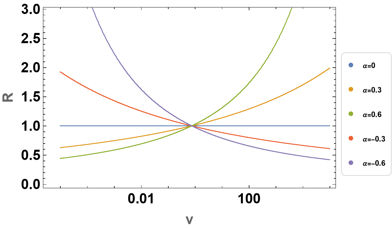
Figure 2: $v(k_{1})(=k_{1}/k_{0})$-dependence of $R$. We fix $m_{0}=2H$ and $\epsilon=0.05/16$, and change the parameter $\alpha$ from $-0.6$ to $0.6$.

Depending on the values of $v$ and $\alpha$, the correction to the power spectrum can either be increased or decreased. Furthermore, we can analytically estimate the leading $v$-dependence of the power spectrum $P_{\zeta}^{(1)}$ as

$$\dfrac{\partial P_{\zeta}^{(1)}}{\partial v}=f_{P}(m_{0})\frac{\sqrt{\epsilon}\alpha}{v}+\order{\epsilon},$$ (4.9)

where $f_{P}(m_{0})$ is a function of $m_{0}$. This $v$ dependence coincides with the behavior derived in general single field inflation scenarios (see e.g., [150]). Note that, although the $v$-dependence is identical, the leading order of slow-roll parameter dependence is different from the general single field case where the leading order is $\order{\epsilon,\eta}$. We also note that the $v$-dependence in Eq. (4.9) is universal as slow-roll correction, while the effect of $\sigma$-field on the inflation background is highly model-dependent. For instance, the power spectrum can often be expanded as $P_{\zeta}=P_{\zeta*}+\varepsilon(t_{\mathrm{exit}}-t_{*})+\order{\varepsilon^{2}}\sim P_{\zeta*}+\varepsilon\log{(k/k_{*})}$ where $\varepsilon$ represents the leading slow-roll order of the theory, e.g., $\varepsilon=\order{\sqrt{\epsilon}}$ in our case.

4.2 Bispectrum

The bispectrum is characterized by the so-called shape function $S$ defined by

$$\left\langle\zeta_{\bf{k}_{1}}\zeta_{\bf{k}_{2}}\zeta_{\bf{k}_{3}}\right\rangle^{\prime}\equiv(2\pi)^{4}\frac{P_{\zeta}^{2}}{\left(k_{1}k_{2}k_{3}\right)^{2}}S.$$ (4.10)

Combining Eq. (2.30) with Eq. (4.5), we derive the shape function

$$S= \ \frac{1}{(2\pi)^{4}}\cdot\frac{1}{P_{\zeta}^{2}}\cdot(2\epsilon M_{\text{Pl}}^{2})^{-\frac{3}{2}}\cdot\left(-2c_{2}c_{3}\right)\cdot\frac{H}{8}\sum_{\mathrm{a},\mathrm{b}=\pm}\left[\frac{k_{1}k_{2}}{k_{3}^{2}}\mathcal{I}_{\mathrm{ab}}^{0,-2}\left(\frac{2k_{3}}{k_{123}},1,v(k_{3})\right)+{\rm{2per.}}\right],$$ (4.11)

where the single soft limit of $\mathcal{I}_{\mathrm{ab}}^{p_{1}p_{2}}$ is described in Eqs. (3.103) and (3.112). In the subsequent subsections, we explore the behavior of the shape function in detail.

4.2.1 Cosmological collider signal at squeezed configuration

Let us consider the configuration $k_{1}=k_{2}$, and define $x\equiv k_{3}/k_{1,2}$ and $v\equiv k_{1}/k_{0}$. Consequently, we can express Eq. (4.11) as

$${S}=\frac{1}{(2\pi)^{4}}\cdot\frac{1}{P_{\zeta}^{2}}\cdot (2\epsilon M_{\text{Pl}}^{2})^{-\frac{3}{2}}\cdot\left(-2c_{2}c_{3}\right)\cdot\frac{H}{8}$$

$$\times\sum_{\mathrm{a},\mathrm{b}=\pm}\left[\frac{1}{x^{2}}\mathcal{I}_{\mathrm{ab}}^{0,-2}\left(\frac{2x}{2+x},1,vx\right)+2x\mathcal{I}_{\mathrm{ab}}^{0,-2}\left(\frac{2}{2+x},1,v\right)\right].$$ (4.12)

In this expression, the squeezed limit $k_{3}\ll k_{1,2}$ corresponds to $x\ll 1$, while the equilateral one $k_{1}\simeq k_{2}\simeq k_{3}$ to $x\simeq 1$.

The squeezed limit of the bispectrum is of particular interest in cosmological collider physics, as specific oscillatory patterns can sharply appear in this limit. In Fig. 3, we present ${S}/c_{2}c_{3}\sqrt{x}$ as a function of $x^{-1}$, with varying values of $\alpha$. Our parameter choices are $v=1$, $m_{0}=2H\ (2.5H)$ for $\alpha>0(<0)$, $\epsilon=0.05/16$, and $M_{\text{Pl}}/H=10^{5}$.

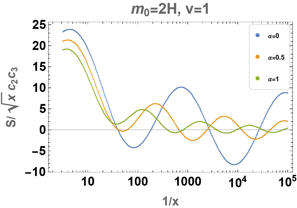
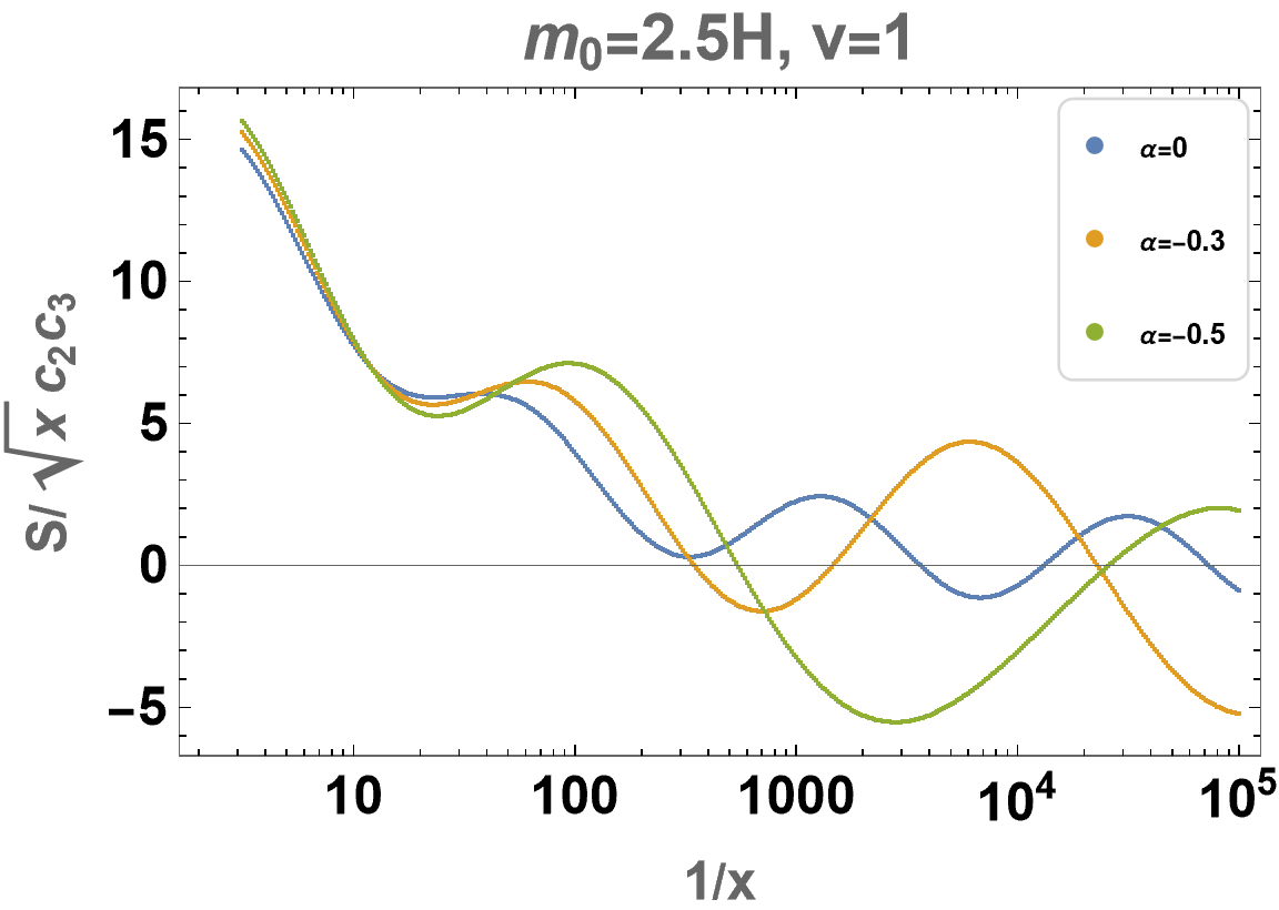
Figure 3: ${S}/c_{2}c_{3}\sqrt{x}$ as a function of $x^{-1}$ with several choices of $\alpha$. Left : Case with $\alpha\geq 0$, that is changed as $0$ (blue), $0.5$ (orange), and $1$ (green). Right : Case with $\alpha\leq 0$, that is changed as $0$ (blue), $-0.3$ (orange), and $-0.5$ (green).

It is readily apparent that both the amplitude and the oscillation frequency exhibit strong dependence on $k_{1}/k_{3}$. For $\alpha>0$, the amplitude experiences damping and the frequency diminish in the squeezed configuration ($x\ll 1$). The opposite behavior is observed for $\alpha<0$. This feature is more prominent for an increased value of $|\alpha|$, and the deviation from a constant mass signal is sufficiently significant to observe. Note that these results are consistent with previous works, including calculations within super-horizon approximation [70] and numerical simulation [86].

The physical interpretation of this signal is clear. In the squeezed limit $x\ll 1$, we are essentially observing the correlation between a long wavelength mode $k_{3}$ and short ones $k_{1,2}$. The long mode exits the horizon earlier than the short ones and evolves on the super-horizon scale $|k_{3}\tau|\ll 1$, schematically represented by

$$v_{k_{3}}(\tau)\sim(-\tau)^{\frac{3}{2}}\left[(-\tau)^{\mathrm{i}\mu}+e^{-\pi\mu}(-\tau)^{-\mathrm{i}\mu}\right],$$ (4.13)

where we showed only $\tau$-dependence of the mode function, disregarding the relative phase of the positive and negative frequency modes. The relative amplitude $e^{-\pi\mu}$ of the positive and negative frequency modes is nothing but (the square root of) the Boltzmann factor responsible for on-shell particle creation relevant to the CC signal. In the present case, $\mu$ exhibits scale dependence due to the horizon crossing time difference. For $\alpha>0\ (<0)$, the mass of $\sigma$ becomes heavier (lighter) than the constant mass scenario due to its time-dependent nature. Consequently, the mode function is more (less) suppressed by the Boltzmann factor $e^{-\pi\mu}$ compared to the constant mass case, leading to a smaller (larger) amplitude and a shorter (longer) wavelength in the oscillatory signal of the bispectrum. Furthermore, the oscillation frequency is scale-dependent accordingly.

4.2.2 Distinction of couplings with inflaton

Recall that the time-dependent mass appears because the non-derivative couplings break the shift symmetry; it is not easy to obtain similar effects from derivative couplings. Therefore, when we observe the specific behavior in the CC signal, such as the damping/enhancement of amplitude and the shrinking/spreading of wavelength in the squeezed limit, it is attributed to these non-derivative (direct) interactions. Moreover, detailed observations of the time-dependent Boltzmann factor associated with non-derivative couplings between the inflaton and the $\sigma$-field allow us to distinguish the form of the interactions. This is obtained from distinctive characteristics in the tail of the “scaling” behavior in the CC signal. We will delve deeper into this aspect in the following discussion.

In the shape function (4.12) with Eqs. (3.103) and (3.112), one can extract the Boltzmann factor for $\mu\gtrsim 1$ with

$$|\Gamma(a+\mathrm{i}b)|\sim e^{-\pi|b|/2},\quad|b|\gtrsim 1,\quad a,b\in\mathbb{R},$$ (4.14)

This reveals that the shape function behaves as

$$S/\sqrt{x}\sim e^{-\pi\mu(x)}x^{\pm\mathrm{i}\mu}+{\rm{c.c.}},$$ (4.15)

in the squeezed limit, $x\ll 1$. Regarding the Boltzmann factor $e^{-\pi\mu(x)}$, it is crucial to emphasize that $\mu$ exhibits $x$-dependence due to the time-dependent mass arising from the coupling to the inflaton, unlike the constant mass situation. Consequently, the amplitude of the CC signal exhibits a scaling behavior in addition to the well-known oscillation, as observed in the previous subsection (see Fig. 3). In case of the linear coupling (4.1), we can estimate the scaling

$$e^{-\pi\mu(x)}\sim e^{-\pi m_{0}/H}\cdot\left(\frac{v}{x}\right)^{-\pi\frac{m_{0}}{H}\sqrt{\frac{\epsilon}{2}}\alpha},$$ (4.16)

as a function of $x$. The left figure of Fig. 4 illustrates the scaling tail of the oscillatory part (orange line) estimated in Eq. (4.16) on the top of the full shape including the background part (4.12). Eq. (4.16) essentially characterizes the scaling behavior in the squeezed limit ($x\ll 1$).

Remarkably, the scaling behavior exhibits dependence on the coupling between the inflaton and the massive field. For example, in the case of a quadratic coupling,

$$g(\phi)=m_{0}^{2}\left(1+\beta\frac{\phi^{2}}{M_{\text{Pl}}^{2}}\right),$$ (4.17)

we obtain

$$e^{-\pi\mu(x)}\sim e^{-\pi m_{0}/H}\cdot e^{-\pi\frac{m_{0}}{H}\cdot\beta\epsilon\left(\log vx\right)\left(\log vx+2\right)}$$ (4.18)

instead of Eq. (4.16). This new formulation represents the amplitude of the corresponding CC signal, as demonstrated in the right panel of Fig. 4, and the scaling behavior ($x$-dependence) differs significantly from the linear case. Therefore, in principle, we can distinguish the coupling $g(\phi)$ through careful observations and analysis of these scaling behaviors.

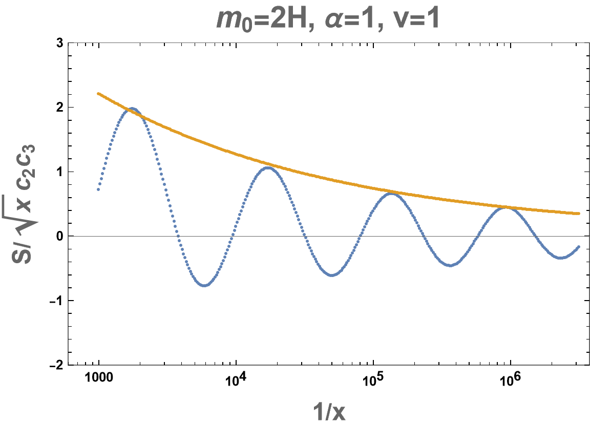
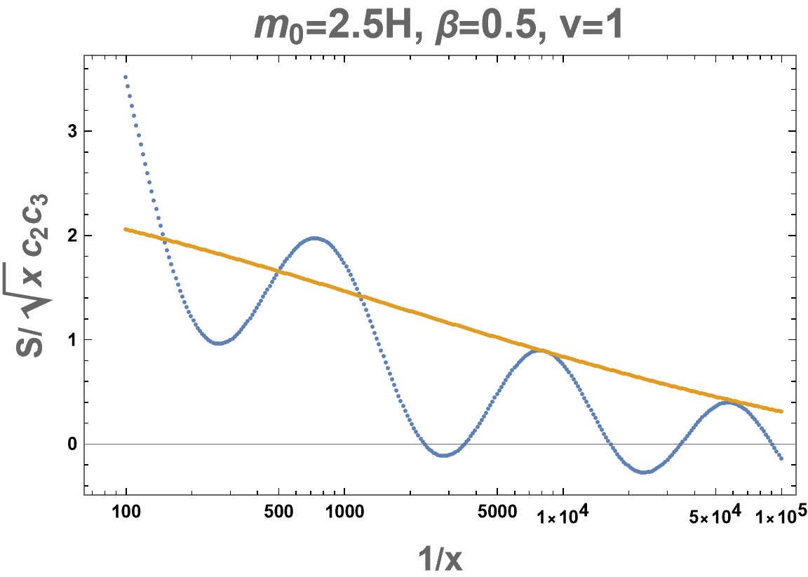
Figure 4: Fitting of the full shape (4.12) (blue line) with scaling function $e^{-\pi\mu(x)}$ (orange line). Left : Linear case (4.1) with Eq. (4.16). Right : Quadratic case (4.17) with (4.18). Parameters are chosen as described in the figure.

It is straightforward to obtain a similar formula for more generic couplings. For example, for a coupling,

$$g(\phi)=m_{0}^{2}\left(1+\alpha_{(n)}\frac{\phi^{n}}{M_{\text{Pl}}^{n}}\right),$$ (4.19)

with $n$ being positive integers, we have the following scaling function,

$$e^{-\pi\mu(x)}\sim e^{-\pi m_{0}/H}\cdot e^{-\pi\frac{m_{0}}{H}\cdot\frac{\alpha_{(n)}}{2}(-\sqrt{2\epsilon})^{n}\left(\log vx\right)^{n-1}\left(\log vx+n\right)},$$ (4.20)

which predicts a different scaling depending on $n$.

4.2.3 Equilateral configuration

While the CC signal in the squeezed configuration is quite essential to extract information about $\sigma$-field, the bispectrum (4.12) exhibits a peak (dominant contribution) at the equilateral limit $x\simeq 1$. Hence, it is equally valuable to investigate the behavior around the equilateral configuration. In our scenario, the magnitude of the shape function or the non-Gaussianity parameter $f_{\text{NL}}$ in the equilateral limit is estimated by using

$$f_{\text{NL}}^{\text{equi}}\sim c_{2}c_{3}\times\order{10},$$ (4.21)

for $\alpha\sim\order{1}$ and $m_{0}\sim\order{H}$.

In Fig. 5, we present plots of ${S}$ for $x\gtrsim 0.1$ (equilateral configuration) varying the interaction strength $\alpha$ (left figure) and the additional scale dependence $v$ (right figure).

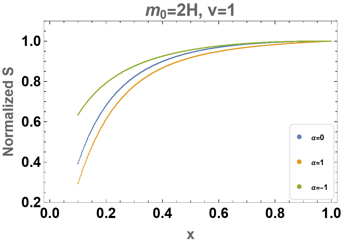
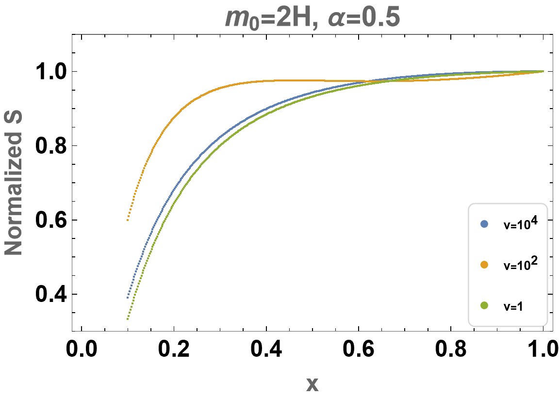
Figure 5: The shape function $S$ as the function of $x$. Here ${S}$ is normalized to have value $1$ at the equilateral limit $x=1$. Left: $\alpha$-dependence with $m_{0}=2H$ and $v=1$ fixed. Right: $v$-dependence with $m_{0}=2H$ and $\alpha=0.5$ fixed.

We find that the values of $\alpha$ and $v$ change the scaling behavior of the bispectrum towards the equilateral configuration. Furthermore, the leading $v$-dependence of the shape function $S$ at $x=1$ is obtained in the same way as the power spectrum. Specifically, $\partial{S}/\partial{v}=f_{S}(m_{0})\sqrt{\epsilon}\alpha/v+\order{\epsilon}$ where $f_{S}(m_{0})$ is a function of $m_{0}$. Unfortunately, for reasons discussed in the subsection of the power spectrum, it is difficult to extract information about the theory from the scale dependence at the exact equilateral configuration.

5 Summary

Our paper provided analytical formulae for the inflationary correlators, specifically two-, three-, and four-point correlation functions, in the presence of a massive scalar field with time-dependent mass. The results are summarized in Eqs. (3.77) and (3.89) for four-point correlators, Eqs. (3.103) and (3.112) for three-point, and Eqs. (3.127) and (3.135) for two-point. The time dependence of mass naturally arises from couplings to the inflaton, and its effects can be significant when the couplings do not respect the shift symmetry of the inflaton, i.e., in the case of non-derivative couplings. The mode function of the massive field (2.17) is analytically given by the Whittaker function under the linear order expansion around the time of horizon crossing for the time-dependence inflaton background, which characterizes the scale dependence of the signal. The analytical formulae for the correlators obtained from the bootstrap method include both the signal (oscillatory) parts and the background (non-oscillatory) parts of the bispectrum as graphically shown in Fig. 3 and 5. The non-oscillatory part of the signal is also crucial for achieving precision in the cosmological collider (CC) program.

As an application, the phenomenological impact of the time dependence on the primordial curvature power spectrum and bispectrum were investigated. Our analysis revealed that the CC signal exhibits the damping/enhancement of amplitude due to the time-dependent (or scale-dependent) Boltzmann factor. The change in amplitude in the CC signal can be readily observed and provide evidence for the time-dependent mass of the massive field. Although this behavior has been qualitatively confirmed in previous numerical studies such as Ref. [86], we quantitatively parameterized this scaling of the amplitude in a simple form (4.20) based on our analytical formulae. By probing the scaling behavior in the tail of the signal, we are able to distinguish couplings between the inflaton and the massive field, which provides a pathway to explore the unknown inflaton sector through the CC signal.

It should be noted that we made an approximation by linearizing the time dependence of the inflaton and omitting the higher-order time dependence. This is merely the approximation made in our study. While extensions beyond linear order present technical challenges in obtaining analytical representations of non-Gaussianity, there are interesting scenarios beyond the scope of our setup, such as CC signals from tachyonic phase transitions [48]. We plan to explore these topics in future work.

Acknowledgments

We thank Lucas Pinol, Yi Wang and Zhong-Zhi Xianyu for valuable discussions and their hospitalities when F.S. stayed at their groups, Dong-Gang Wang and Sébastien Renaux-Petel for valuable discussions in Gravity 2023, YITP and COSMO 2023, IFT, and Yuhang Zhu for valuable discussions. S.A. is supported by IBS under the project code, IBS-R018-D1. T.N. is supported in part by JSPS KAKENHI Grant No. 20H01902 and No. 22H01220, and MEXT KAKENHI Grant No. 21H05184 and No. 23H04007. F.S. is supported by financial aid from the Center for the Theoretical Physics of the Universe, Institute for Basic Science, financial aid from the Advanced Research Center for Quantum Physics and Nanoscience, Tokyo Institute of Technology, and JSPS Grant-in-Aid for Scientific Research No. 23KJ0938. M.Y. is supported by IBS under the project code IBS-R018-D3 and JSPS Grant-in-Aid for Scientific Research No. JP21H01080.

Appendix A Seed integral with the Mellin–Barnes representation

In this appendix, we present a direct integration method for the seed integral (2.29), based on the technique utilized in Ref. [128, 132] which makes use of the Mellin–Barnes representation of Whittaker function,

$$\mathrm{W}_{\kappa,\nu}(z) =e^{z/2}\int_{-\mathrm{i}\infty}^{+\mathrm{i}\infty}\frac{\mathrm{d}s}{2\pi\mathrm{i}}\Gamma\left[\begin{array}[]{c}s-\nu,s+\nu\\ s-\kappa+\frac{1}{2}\end{array}\right]z^{-s+1/2},$$ (A.3)

$$\mathrm{~{}W}_{\kappa,\nu}(z) =e^{-z/2}\int_{-\mathrm{i}\infty}^{+\mathrm{i}\infty}\frac{\mathrm{d}s}{2\pi\mathrm{i}}\Gamma\left[\begin{array}[]{c}s-\nu,s+\nu,-s-\kappa+\frac{1}{2}\\ \frac{1}{2}-\kappa-\nu,\frac{1}{2}-\kappa+\nu\end{array}\right]z^{-s+1/2}.$$ (A.6)

As a reminder, the notation used in the paper is as follows:

$${}_{p}\mathcal{F}_{q}\left[\begin{array}[]{c|c}a_{1},\cdots,a_{p}\\ b_{1},\cdots,b_{q}\end{array}\ z\right]\equiv\Gamma\left[\begin{array}[]{c}a_{1},\cdots,a_{p}\\ b_{1},\cdots,b_{q}\end{array}\right]{}_{p}\mathrm{F}_{q}\left[\begin{array}[]{c|c}a_{1},\cdots,a_{p}\\ b_{1},\cdots,b_{q}\end{array}\ z\right],$$ (A.13)

where ${}_{p}\mathrm{F}_{q}$ represents the (generalized) hypergeometric function, and the products of gamma functions are abbreviated as

$$\Gamma\left[z_{1},\cdots,z_{m}\right]\equiv\Gamma\left(z_{1}\right)\cdots\Gamma\left(z_{m}\right),$$ (A.14)

$$\Gamma\left[\begin{array}[]{c}z_{1},\cdots,z_{m}\\ w_{1},\cdots,w_{n}\end{array}\right]\equiv\frac{\Gamma\left(z_{1}\right)\cdots\Gamma\left(z_{m}\right)}{\Gamma\left(w_{1}\right)\cdots\Gamma\left(w_{n}\right)}.$$ (A.17)

Opposite sign seed $\mathcal{I}_{\pm\mp}^{p_{1}p_{2}}$

To compute the opposite sign seed integral $\mathcal{I}_{\pm\mp}^{p_{1}p_{2}}$, we first express the propagators $D_{\pm\mp}$ using Eq. (A.6):

$$D_{\pm\mp}\left(k;\tau_{1},\tau_{2}\right)= \ \frac{e^{\pi\kappa}}{2k}H^{2}(\tau_{1}\tau_{2})W_{\pm\mathrm{i}\kappa,\mp\mathrm{i}\mu}(\mp 2\mathrm{i}k\tau_{1})W_{\mp\mathrm{i}\kappa,\pm\mathrm{i}\mu}(\pm 2\mathrm{i}k\tau_{2})$$

$$= \ \frac{e^{\pi\kappa}}{2\pi^{2}}H^{2}e^{\pm\mathrm{i}k\left(\tau_{1}-\tau_{2}\right)}\left[\cosh\left(2\pi\kappa\right)+\cosh(2\pi\mu)\right]$$

$$\times\int_{-\mathrm{i}\infty}^{+\mathrm{i}\infty}\frac{\mathrm{d}s_{1}}{2\pi\mathrm{i}}\frac{\mathrm{d}s_{2}}{2\pi\mathrm{i}}e^{\mp\mathrm{i}\pi\left(s_{1}-s_{2}\right)/2}\left(2k\right)^{-s_{12}}\left(-\tau_{1}\right)^{-s_{1}+3/2}\left(-\tau_{2}\right)^{-s_{2}+3/2}$$

$$\times\Gamma\left[-s_{1}+\frac{1}{2}\mp\mathrm{i}\kappa,-s_{2}+\frac{1}{2}\pm\mathrm{i}\kappa,s_{1}-\mathrm{i}\mu,s_{1}+\mathrm{i}\mu,s_{2}-\mathrm{i}\mu,s_{2}+\mathrm{i}\mu\right],$$ (A.18)

where $s_{12}=s_{1}+s_{2}$. Substituting this expression into $\mathcal{I}_{\pm\mp}^{p_{1}p_{2}}$ enables us to carry out the $\tau_{1,2}$-integral, resulting in

$$\mathcal{I}_{\pm\mp}^{p_{1}p_{2}}= \ \frac{e^{\pi\kappa(k_{s})}}{2\pi^{2}}H^{2}\left[\cosh\left(2\pi\kappa(k_{s})\right)+\cosh(2\pi\mu)\right]\left(\frac{u_{1}}{2}\right)^{5/2+p_{1}}\left(\frac{u_{2}}{2}\right)^{5/2+p_{2}}e^{\mp\mathrm{i}\pi\left(p_{1}-p_{2}\right)/2}$$

$$\times\int_{-\mathrm{i}\infty}^{\mathrm{i}\infty}\frac{\mathrm{d}s_{1}}{2\pi\mathrm{i}}\frac{\mathrm{d}s_{2}}{2\pi\mathrm{i}}u_{1}^{-s_{1}}u_{2}^{-s_{2}}\Gamma\left[p_{1}+\frac{5}{2}-s_{1},p_{2}+\frac{5}{2}-s_{2}\right]$$

$$\times\Gamma\left[-s_{1}+\frac{1}{2}\mp\mathrm{i}\kappa(k_{s}),-s_{2}+\frac{1}{2}\pm\mathrm{i}\kappa(k_{s}),s_{1}-\mathrm{i}\mu,s_{1}+\mathrm{i}\mu,s_{2}-\mathrm{i}\mu,s_{2}+\mathrm{i}\mu\right],$$ (A.19)

where

$$u_{1}\equiv\frac{2r_{1}}{1+r_{1}},\quad u_{2}\equiv\frac{2r_{2}}{1+r_{2}},$$ (A.20)

and we explicitly denote $k_{s}$ dependence in $\kappa(k_{s})$ (see Eq. (2.16) with Eq. (2.9)). The integration over $s_{i}$ can be computed using the residue theorem. We close the contours from the left with a large semicircle and pick up the poles $s_{i}=-n_{i}\pm\mathrm{i}\mu$ with $n_{i}$ to be non-negative integers. This process allows us to express the seed integral as

$$\mathcal{I}_{\pm\mp}^{p_{1}p_{2}}= \ \frac{e^{\pi\kappa(k_{s})}}{2\pi^{2}}H^{2}\left[\cosh\left(2\pi\kappa(k_{s})\right)+\cosh(2\pi\mu)\right]\left(\frac{u_{1}}{2}\right)^{5/2+p_{1}}\left(\frac{u_{2}}{2}\right)^{5/2+p_{2}}e^{\mp\mathrm{i}\pi\left(p_{1}-p_{2}\right)/2}$$

$$\times\sum_{n_{1}=0}^{\infty}\left\{\frac{(-1)^{n_{1}}}{n_{1}!}u_{1}^{n_{1}+\mathrm{i}\mu}\Gamma\left[n_{1}+p_{1}+\frac{5}{2}+\mathrm{i}\mu,n_{1}+\mathrm{i}\mu+\frac{1}{2}\mp\mathrm{i}\kappa(k_{s}),-n_{1}-2\mathrm{i}\mu\right]+(\mu\rightarrow-\mu)\right\}$$

$$\times\sum_{n_{2}=0}^{\infty}\left\{\frac{(-1)^{n_{2}}}{n_{2}!}u_{2}^{n_{2}+\mathrm{i}\mu}\Gamma\left[n_{2}+p_{2}+\frac{5}{2}+\mathrm{i}\mu,n_{2}+\mathrm{i}\mu+\frac{1}{2}\pm\mathrm{i}\kappa(k_{s}),-n_{2}-2\mathrm{i}\mu\right]+(\mu\rightarrow-\mu)\right\},$$ (A.21)

and the summations can be performed explicitly, leading to

$$\mathcal{I}_{\pm\mp}^{p_{1}p_{2}}= \ \frac{e^{\pi\kappa(k_{s})}}{2\pi^{2}}H^{2}\left[\cosh\left(2\pi\kappa(k_{s})\right)+\cosh(2\pi\mu)\right]e^{\mp\mathrm{i}\pi\left(p_{1}-p_{2}\right)/2}$$

$$\times\left[\mathrm{G}_{\mp\mathrm{i}\kappa(k_{s}),\mu}^{p_{1}}\left(u_{1}\right)u_{1}^{\mathrm{i}\mu}+\mathrm{G}_{\mp\mathrm{i}\kappa(k_{s}),-\mu}^{p_{1}}\left(u_{1}\right)u_{1}^{-\mathrm{i}\mu}\right]\left[\mathrm{G}_{\pm\mathrm{i}\kappa(k_{s}),\mu}^{p_{2}}\left(u_{2}\right)u_{2}^{\mathrm{i}\mu}+\mathrm{G}_{\pm\mathrm{i}\kappa(k_{s}),-\mu}^{p_{2}}\left(u_{2}\right)u_{2}^{-\mathrm{i}\mu}\right],$$ (A.22)

where

$$\mathrm{G}_{\pm\mathrm{i}\kappa(k_{s}),\mu}^{p}(u)\equiv\mathrm{i}\pi\operatorname{csch}(2\pi\mu)\left(\frac{u}{2}\right)^{5/2+p}{}_{2}\mathcal{F}_{1}\left[\begin{array}[]{c|c}\frac{5}{2}+p+\mathrm{i}\mu,\frac{1}{2}+\mathrm{i}\mu\pm\mathrm{i}\kappa(k_{s})\\ 1+2\mathrm{i}\mu\end{array}\ u\right].$$ (A.25)

In particular, in the hierarchical collapsed limit $u_{1}\ll u_{2}\ll 1$, we obtain

$$\lim_{u_{1}\ll u_{2}\ll 1}\mathcal{I}_{\pm\mp}^{p_{1}p_{2}}=\sum_{\mathrm{a,b}=\pm}\tilde{\mathcal{C}}_{\pm\mp\mid\mathrm{ab}}\ \tilde{\mathcal{U}}_{\pm\mid\mathrm{a}}^{p_{1}}\left(u_{1}\right)\tilde{\mathcal{U}}_{\mp\mid\mathrm{b}}^{p_{2}}\left(u_{2}\right),$$ (A.26)

where

$$\tilde{\mathcal{C}}_{\pm\mp\mid++}=\tilde{\mathcal{C}}_{\pm\mp\mid+-}=\tilde{\mathcal{C}}_{\pm\mp\mid-+}=\tilde{\mathcal{C}}_{\pm\mp\mid--}=\frac{e^{\pi\kappa}}{2\pi^{2}}H^{2}\left[\cosh\left(2\pi\kappa(k_{s})\right)+\cosh(2\pi\mu)\right]e^{\mp\mathrm{i}\pi\left(p_{1}-p_{2}\right)/2},$$ (A.27)

and

$$\tilde{\mathcal{U}}_{\mathrm{a}\mid\mathrm{b}}^{p}(u)=\operatorname{iab}2^{\mathrm{iab}\mu}\pi\operatorname{csch}(2\pi\mu)\left(\frac{u}{2}\right)^{5/2+p+\mathrm{iab}\mu}\Gamma\left[\begin{array}[]{c}\frac{5}{2}+p+\operatorname{iab}\mu,\frac{1}{2}-\operatorname{ia}\kappa+\operatorname{iab}\mu\\ 1+2\operatorname{iab}\mu\end{array}\right].$$ (A.30)

Same sign seed $\mathcal{I}_{\pm\pm}^{p_{1}p_{2}}$

For the same sign seed integral, we adopt a division of the propagators in the same way employed in [128, 132],

$$D_{\pm\pm}\left(k;\tau_{1},\tau_{2}\right)=D_{\gtrless}\left(k;\tau_{1},\tau_{2}\right)+\left[D_{\lessgtr}\left(k;\tau_{1},\tau_{2}\right)-D_{\gtrless}\left(k;\tau_{1},\tau_{2}\right)\right]\theta\left(\tau_{2}-\tau_{1}\right),$$ (A.31)

and accordingly, we define

$$\mathcal{I}_{\pm\pm}^{p_{1}p_{2}}=\mathcal{I}_{\pm\pm,\mathrm{F},>}^{p_{1}p_{2}}+\mathcal{I}_{\pm\pm,\mathrm{TO},>}^{p_{1}p_{2}},\quad\left(r_{1}<r_{2}\right)$$ (A.32)

where the factorized (F) integral $\mathcal{I}_{\pm\pm,\mathrm{F},>}^{p_{1}p_{2}}$ and the time-ordered (TO) integral $\mathcal{I}_{\pm\pm,\mathrm{TO},>}^{p_{1}p_{2}}$ are expressed as

$$\mathcal{I}_{\pm\pm,\mathrm{F},>}^{p_{1}p_{2}}= -k_{s}^{5+p_{12}}\int_{-\infty}^{0}\mathrm{~{}d}\tau_{1}\mathrm{~{}d}\tau_{2}\left(-\tau_{1}\right)^{p_{1}}\left(-\tau_{2}\right)^{p_{2}}e^{\pm\mathrm{i}\left(k_{12}\tau_{1}+k_{34}\tau_{2}\right)}D_{\gtrless}\left(k_{s};\tau_{1},\tau_{2}\right),$$ (A.33)

$$\mathcal{I}_{\pm\pm,\mathrm{TO},>}^{p_{1}p_{2}}= -k_{s}^{5+p_{12}}\int_{-\infty}^{0}\mathrm{~{}d}\tau_{2}\int_{-\infty}^{\tau_{2}}\mathrm{~{}d}\tau_{1}\left(-\tau_{1}\right)^{p_{1}}\left(-\tau_{2}\right)^{p_{2}}e^{\pm\mathrm{i}\left(k_{12}\tau_{1}+k_{34}\tau_{2}\right)}$$

$$\times\left[D_{\lessgtr}\left(k_{s};\tau_{1},\tau_{2}\right)-D_{\gtrless}\left(k_{s};\tau_{1},\tau_{2}\right)\right].$$ (A.34)

Let us start from the factorized (F) integral $\mathcal{I}_{\pm\pm,\mathrm{F},>}$. We rewrite the propagators $D_{\pm\mp}$ using the Mellin–Barnes representations Eqs. (A.3) and (A.6):

$$D_{\pm\mp}\left(k;\tau_{1},\tau_{2}\right)= \ \frac{e^{\pi\kappa}H^{2}}{\pi\Gamma\left[\frac{1}{2}-\mathrm{i}\mu\pm\mathrm{i}\kappa,\frac{1}{2}+\mathrm{i}\mu\pm\mathrm{i}\kappa\right]}e^{\mp\mathrm{i}k\left(\tau_{1}+\tau_{2}\right)}$$

$$\times\int_{-\mathrm{i}\infty}^{\mathrm{i}\infty}\frac{\mathrm{d}s_{1}}{2\pi\mathrm{i}}\frac{\mathrm{d}s_{2}}{2\pi\mathrm{i}}e^{\mp\mathrm{i}\pi\left(s_{1}-s_{2}\right)/2}\cos\pi\left(s_{1}\mp\mathrm{i}\kappa\right)\left(2k\right)^{-s_{12}}\left(-\tau_{1}\right)^{-s_{1}+3/2}\left(-\tau_{2}\right)^{-s_{2}+3/2}$$

$$\times\Gamma\left[-s_{1}+\frac{1}{2}\pm\mathrm{i}\kappa,-s_{2}+\frac{1}{2}\pm\mathrm{i}\kappa,s_{1}-\mathrm{i}\mu,s_{1}+\mathrm{i}\mu,s_{2}-\mathrm{i}\mu,s_{2}+\mathrm{i}\mu\right],$$ (A.35)

which leads to the subsequent expression of $\mathcal{I}_{\pm\pm,\mathrm{F},>}$ after the $\tau_{i}$-integration,

$$\mathcal{I}_{\pm\pm,\mathrm{F},>}^{p_{1}p_{2}}= \ \frac{\pm\mathrm{i}e^{\pi\kappa(k_{s})}H^{2}}{\pi\Gamma\left[\frac{1}{2}-\mathrm{i}\mu\mp\mathrm{i}\kappa(k_{s}),\frac{1}{2}+\mathrm{i}\mu\mp\mathrm{i}\kappa(k_{s})\right]}\left(\frac{u_{1}}{2}\right)^{5/2+p_{1}}\left(\frac{u_{2}}{2}\right)^{5/2+p_{2}}e^{\mp\mathrm{i}\pi\left(p_{1}+p_{2}\right)/2}$$

$$\times\int_{-\mathrm{i}\infty}^{\mathrm{i}\infty}\frac{\mathrm{d}s_{1}}{2\pi\mathrm{i}}\frac{\mathrm{d}s_{2}}{2\pi\mathrm{i}}e^{\pm\mathrm{i}\pi s_{1}}\cos\pi\left(s_{1}\pm\mathrm{i}\kappa(k_{s})\right)u_{1}^{-s_{1}}u_{2}^{-s_{2}}\Gamma\left[p_{1}+\frac{5}{2}-s_{1},p_{2}+\frac{5}{2}-s_{2}\right]$$

$$\times\Gamma\left[-s_{1}+\frac{1}{2}\mp\mathrm{i}\kappa(k_{s}),-s_{2}+\frac{1}{2}\mp\mathrm{i}\kappa(k_{s}),s_{1}-\mathrm{i}\mu,s_{1}+\mathrm{i}\mu,s_{2}-\mathrm{i}\mu,s_{2}+\mathrm{i}\mu\right].$$ (A.36)

The integration over $s_{i}$ and the summation of the residues can be executed following a similar procedure, and we obtain

$$\mathcal{I}_{\pm\pm,\mathrm{F},>}^{p_{1}p_{2}}= \ \frac{\pm\mathrm{i}e^{\pi\kappa(k_{s})}H^{2}}{\pi\Gamma\left[\frac{1}{2}-\mathrm{i}\mu\mp\mathrm{i}\kappa(k_{s}),\frac{1}{2}+\mathrm{i}\mu\mp\mathrm{i}\kappa(k_{s})\right]}\left(\frac{u_{1}}{2}\right)^{5/2+p_{1}}\left(\frac{u_{2}}{2}\right)^{5/2+p_{2}}e^{\mp\mathrm{i}\pi\left(p_{1}+p_{2}\right)/2}$$

$$\times\sum_{n_{1}=0}^{\infty}\left\{\frac{(-1)^{n_{1}}}{n_{1}!}e^{\mp\mathrm{i}\pi(n_{1}+\mathrm{i}\mu)}\cos\pi\left(-n_{1}-\mathrm{i}\mu\pm\mathrm{i}\kappa(k_{s})\right)u_{1}^{n_{1}+\mathrm{i}\mu}\right.$$

$$\times\left.\Gamma\left[-n_{1}-2\mathrm{i}\mu,n_{1}+\mathrm{i}\mu+\frac{1}{2}\mp\mathrm{i}\kappa(k_{s}),n_{1}+\mathrm{i}\mu+p_{1}+\frac{5}{2}\right]+(\mu\rightarrow-\mu)\right\}$$

$$\times\sum_{n_{2}=0}^{\infty}\left\{\frac{(-1)^{n_{2}}}{n_{2}!}u_{2}^{n_{2}+\mathrm{i}\mu}\Gamma\left[-n_{2}-2\mathrm{i}\mu,n_{2}+\mathrm{i}\mu+\frac{1}{2}\mp\mathrm{i}\kappa(k_{s}),n_{2}+\mathrm{i}\mu+p_{2}+\frac{5}{2}\right]+(\mu\rightarrow-\mu)\right\}$$ (A.37)

$$= \ \frac{\pm\mathrm{i}e^{\pi\kappa(k_{s})}H^{2}}{\pi\Gamma\left[\frac{1}{2}-\mathrm{i}\mu\mp\mathrm{i}\kappa(k_{s}),\frac{1}{2}+\mathrm{i}\mu\mp\mathrm{i}\kappa(k_{s})\right]}e^{\mp\mathrm{i}\pi\left(p_{1}+p_{2}\right)/2}$$

$$\times\left[e^{\pm\pi\mu}\cosh\pi\left(\mu\mp\kappa(k_{s})\right)\mathrm{G}_{\mp\mathrm{i}\kappa(k_{s}),\mu}^{p_{1}}\left(u_{1}\right)u_{1}^{\mathrm{i}\mu}+e^{\mp\pi\mu}\cosh\pi\left(\mu\pm\kappa(k_{s})\right)\mathrm{G}_{\mp\mathrm{i}\kappa(k_{s}),-\mu}^{p_{1}}\left(u_{1}\right)u_{1}^{-\mathrm{i}\mu}\right]$$

$$\times\left[\mathrm{G}_{\mp\mathrm{i}\kappa(k_{s}),\mu}^{p_{2}}\left(u_{2}\right)u_{2}^{\mathrm{i}\mu}+\mathrm{G}_{\mp\mathrm{i}\kappa(k_{s}),-\mu}^{p_{2}}\left(u_{2}\right)u_{2}^{-\mathrm{i}\mu}\right],$$ (A.38)

where the $G$-function is defined in Eq. (A.25).

In the same manner, The time-ordered (TO) integral $\mathcal{I}_{\pm\pm,\mathrm{TO},>}^{p_{1}p_{2}}$ can be transformed to

$$\mathcal{I}_{++,\mathrm{TO},>}^{p_{1}p_{2}}= \ \frac{\mathrm{i}e^{\pi\kappa(k_{s})}H^{2}}{\pi\Gamma\left[\frac{1}{2}-\mathrm{i}\mu-\mathrm{i}\kappa(k_{s}),\frac{1}{2}+\mathrm{i}\mu-\mathrm{i}\kappa(k_{s})\right]}\frac{e^{-\mathrm{i}\pi\left(p_{1}+p_{2}\right)/2}}{2^{5+p_{1}+p_{2}}}\int_{-\mathrm{i}\infty}^{+\mathrm{i}\infty}\frac{\mathrm{d}s_{1}}{2\pi\mathrm{i}}\frac{\mathrm{d}s_{2}}{2\pi\mathrm{i}}$$

$$\times\left[e^{\mathrm{i}\pi s_{2}}\cos\pi\left(s_{2}+\mathrm{i}\kappa(k_{s})\right)-e^{\mathrm{i}\pi s_{1}}\cos\pi\left(s_{1}+\mathrm{i}\kappa(k_{s})\right)\right]u_{1}^{-s_{12}+5+p_{1}+p_{2}}$$

$$\times\Gamma\left[-s_{1}+\frac{1}{2}-\mathrm{i}\kappa(k_{s}),-s_{2}+\frac{1}{2}-\mathrm{i}\kappa(k_{s}),s_{1}-\mathrm{i}\mu,s_{1}+\mathrm{i}\mu,s_{2}-\mathrm{i}\mu,s_{2}+\mathrm{i}\mu\right]$$

$$\times{}_{2}\mathcal{F}_{1}\left[\begin{array}[]{c|c}p_{2}+\frac{5}{2}-s_{2},p_{1}+p_{2}+5-s_{12}\\ p_{2}+\frac{7}{2}-s_{2}\end{array}-\frac{u_{1}}{u_{2}}\right]$$ (A.41)

by utilizing Eq. (A.35) and the integration formula

$$\int_{-\infty}^{0}\mathrm{~{}d}\tau_{2}\int_{-\infty}^{\tau_{2}}\mathrm{~{}d}\tau_{1}e^{\pm\left(\mathrm{i}k_{12}\tau_{1}+\mathrm{i}k_{34}\tau_{2}\right)}\left(-\tau_{1}\right)^{p-1}\left(-\tau_{2}\right)^{q-1}$$

$$\qquad\qquad\qquad=e^{\mp\mathrm{i}(p+q)\frac{\pi}{2}}k_{12}^{-p-q}{}_{2}\mathcal{F}_{1}\left[\begin{array}[]{c|c}q,p+q\\ 1+q\end{array}-\frac{k_{34}}{k_{12}}\right].$$ (A.44)

Subsequently, the complex $s_{i}$-integral leads to

$$\mathcal{I}_{++,\mathrm{TO},>}^{p_{1}p_{2}}= \ \frac{\mathrm{i}H^{2}e^{-\mathrm{i}\pi\left(p_{1}+p_{2}\right)/2}}{2^{5+p_{1}+p_{2}}}\sum_{n_{1},n_{2}=0}^{\infty}\frac{(-1)^{n_{12}}}{n_{1}!n_{2}!}u_{1}^{n_{12}+5+p_{1}+p_{2}}$$

$$\times\left\{\frac{1}{2\mu}\left(\frac{1}{2}-\mathrm{i}\mu-\mathrm{i}\kappa(k_{s})\right)_{n_{1}}\left(\frac{1}{2}+\mathrm{i}\mu-\mathrm{i}\kappa(k_{s})\right)_{n_{2}}(2\mathrm{i}\mu)_{-n_{1}}(-2\mathrm{i}\mu)_{-n_{2}}\right.$$

$$\left.\times{}_{2}\mathcal{F}_{1}\left[\begin{array}[]{c|c}n_{2}+p_{2}+\frac{5}{2}+\mathrm{i}\mu,n_{12}+p_{1}+p_{2}+5\\ n_{2}+p_{2}+\frac{7}{2}+\mathrm{i}\mu\end{array}-\frac{u_{1}}{u_{2}}\right]+(\mu\rightarrow-\mu)\right\},$$ (A.47)

where $(z)_{n}\equiv\Gamma[z+n]/\Gamma[z]$ denotes the Pochhammer symbol. The minus sign seed $\mathcal{I}_{--,\mathrm{TO},>}^{p_{1}p_{2}}$ is obtained by taking a conjugate of Eq. (A.47). In contrast to the previous cases, performing the double summation presented above poses technical challenges.

The hierarchical collapsed limit ($u_{1}\ll u_{2}\ll 1$) of $\mathcal{I}_{\pm\pm}^{p_{1}p_{2}}$ enables us to determine the integration constants appearing in Section 3. Under the limit, the dominant contribution comes from the poles with $n_{1,2}=0$ in Eqs. (A.37) and (A.47). Additionally, $\mathcal{I}_{++,\mathrm{TO},>}^{p_{1}p_{2}}$ is subdominant in comparison to $\mathcal{I}_{\pm\pm,\mathrm{F},>}^{p_{1}p_{2}}$. Combining these evaluations, we obtain

$$\lim_{u_{1}\ll u_{2}\ll 1}\mathcal{I}_{\pm\pm}^{p_{1}p_{2}}=\sum_{\mathrm{a},\mathrm{b}=\pm}\tilde{\mathcal{C}}_{\pm\pm\mid\mathrm{ab}}\ \tilde{\mathcal{U}}_{\pm\mid\mathrm{a}}^{p_{1}}\left(u_{1}\right)\tilde{\mathcal{U}}_{\pm\mid\mathrm{b}}^{p_{2}}\left(u_{2}\right),$$ (A.48)

where

$$\tilde{\mathcal{C}}_{\pm\pm\mid++}=\tilde{\mathcal{C}}_{\pm\pm\mid+-}=\frac{\pm\mathrm{i}e^{\pi\left(\kappa(k_{s})+\mu\right)}\cosh\pi\left(-\mu+\kappa(k_{s})\right)H^{2}}{\pi\Gamma\left[\frac{1}{2}-\mathrm{i}\mu\mp\mathrm{i}\kappa(k_{s}),\frac{1}{2}+\mathrm{i}\mu\mp\mathrm{i}\kappa(k_{s})\right]}e^{\mp\mathrm{i}\pi\left(p_{1}+p_{2}\right)/2},$$ (A.49)

$$\tilde{\mathcal{C}}_{\pm\pm\mid-+}=\tilde{\mathcal{C}}_{\pm\pm\mid--}=\frac{\pm\mathrm{i}e^{\pi\left(\kappa(k_{s})-\mu\right)}\cosh\pi\left(\mu+\kappa(k_{s})\right)H^{2}}{\pi\Gamma\left[\frac{1}{2}-\mathrm{i}\mu\mp\mathrm{i}\kappa(k_{s}),\frac{1}{2}+\mathrm{i}\mu\mp\mathrm{i}\kappa(k_{s})\right]}e^{\mp\mathrm{i}\pi\left(p_{1}+p_{2}\right)/2}.$$ (A.50)

Note that we confirmed that our outcomes (A.19), (A.38), and (A.47) are consistent with the constant mass results of Refs. [128, 132] in the limit $\kappa\rightarrow 0$, as described in the following appendix in detail.

Appendix B Constant Mass Limit

In case where the coupling (2.1) is constant, $g(\phi)=m_{0}^{2}$, which corresponds to $\kappa\rightarrow 0$, the seed integrals with single soft limit, Eqs. (3.103) and (3.112), should reproduce the results for the constant mass scenario presented in Ref. [128, 132]. Since the mode function of the massive field $\sigma$ for the constant mass is expressed by the Hankel function (see Eq. (2.18)) whereas our case is the Whittaker function (see Eq. (2.17)), this limit provides a non-trivial consistency check.

In the subsequent discussion, we frequently use the following formulae for the Gamma function:

$$\Gamma(-z)\Gamma(z+1)=-\frac{\pi}{\sin\pi z},$$ (B.1)

$$\Gamma(2z)=\frac{2^{2z-1}}{\sqrt{\pi}}\Gamma(z)\Gamma\left(z+\frac{1}{z}\right).$$ (B.2)

In the limit $\kappa\rightarrow 0$, Eqs. (3.103) and (3.112) are reduced to

$$\mathcal{I}_{\pm\mp}^{p_{1}p_{2}}(u_{1},1,v(k_{3}))/H^{2}=\frac{e^{\mp\mathrm{i}\frac{\pi}{2}\bar{p}_{12}}}{2^{7/2+p_{2}}\pi^{1/2}}\Gamma\left[\begin{array}[]{c}\frac{5}{2}+p_{2}-\mathrm{i}\mu,\frac{5}{2}+p_{2}+\mathrm{i}\mu\\ 3+p_{2}\end{array}\right]\left[\mathcal{Y}_{+}^{p_{1}}(u)+\mathcal{Y}_{-}^{p_{1}}(u)\right],$$ (B.5)

$$\mathcal{I}_{\pm\pm}^{p_{1}p_{2}}(u_{1},1,v(k_{3}))/H^{2}$$

$$\qquad=\frac{e^{\mp\mathrm{i}\frac{\pi}{2}p_{12}}\Gamma\left(5+p_{12}\right)u_{1}^{5+p_{12}}}{2^{5+p_{12}}\left[\left(\frac{5}{2}+p_{2}\right)^{2}+\mu^{2}\right]}{}_{3}\mathrm{F}_{2}\left[\begin{array}[]{c|c}1,3+p_{2},5+p_{12}\\ \frac{7}{2}+p_{2}-\mathrm{i}\mu,\frac{7}{2}+p_{2}+\mathrm{i}\mu\end{array}\ u_{1}\right]$$ (B.8)

$$\qquad+\frac{\pm\mathrm{i}e^{\mp\mathrm{i}\frac{\pi}{2}p_{12}}}{2^{7/2+p_{2}}\pi^{1/2}}\Gamma\left[\begin{array}[]{c}\frac{5}{2}+p_{2}-\mathrm{i}\mu,\frac{5}{2}+p_{2}+\mathrm{i}\mu\\ 3+p_{2}\end{array}\right]\left[e^{\pi\mu}\mathcal{Y}_{\pm}^{p_{1}}(u_{1})+e^{-\pi\mu}\mathcal{Y}_{\mp}^{p_{1}}(u_{1})\right],$$ (B.11)

respectively, where

$$\mathcal{Y}_{\pm}^{p}(u)\equiv 2^{\mp\mathrm{i}\mu}\left(\frac{u}{2}\right)^{5/2+p\pm\mathrm{i}\mu}\Gamma\left[\frac{5}{2}+p\pm\mathrm{i}\mu,\mp\mathrm{i}\mu\right]{}_{2}\mathrm{F}_{1}\left[\begin{array}[]{c|c}\frac{5}{2}+p\pm\mathrm{i}\mu,\frac{1}{2}\pm\mathrm{i}\mu\\ 1\pm 2\mathrm{i}\mu\end{array}\ u\right].$$ (B.14)

These equations are in agreement with the results of Ref. [132].

In the same way, for the seed integrals with double soft limit (Eqs.(3.127) and (3.135)), we can express them in the limit $\kappa\rightarrow 0$ as follows:

$$\mathcal{I}_{\pm\mp}^{p_{1}p_{2}}(1,1,v(k_{3}))/H^{2}=\frac{e^{\mp\mathrm{i}\frac{\pi}{2}\bar{p}_{12}}}{2^{5+p_{12}}}\Gamma\left[\begin{array}[]{c}\frac{5}{2}+p_{1}-\mathrm{i}\mu,\frac{5}{2}+p_{1}+\mathrm{i}\mu,\frac{5}{2}+p_{2}-\mathrm{i}\mu,\frac{5}{2}+p_{2}+\mathrm{i}\mu\\ 3+p_{1},3+p_{2}\end{array}\right],$$ (B.17)

and

$$\mathcal{I}_{\pm\pm}^{p_{1}p_{2}}(1,1,v(k_{3}))/H^{2}$$

$$=\frac{\pm\mathrm{i}e^{\mp\mathrm{i}\frac{\pi}{2}p_{12}}e^{-\pi\mu}}{2^{5+p_{12}}}\Gamma\left[\begin{array}[]{c}\frac{5}{2}+p_{1}-\mathrm{i}\mu,\frac{5}{2}+p_{1}+\mathrm{i}\mu,\frac{5}{2}+p_{2}-\mathrm{i}\mu,\frac{5}{2}+p_{2}+\mathrm{i}\mu\\ 3+p_{1},3+p_{2}\end{array}\right]$$ (B.20)

$$-\frac{e^{\mp\mathrm{i}\frac{\pi}{2}p_{12}}}{2^{p_{12}+5}}\Gamma\left[\begin{array}[]{c}\frac{5}{2}+p_{2}\pm\mathrm{i}\mu,\frac{5}{2}+p_{1}\pm\mathrm{i}\mu\\ \frac{1}{2}\pm\mathrm{i}\mu\end{array}\right]{}_{3}\mathcal{F}_{2}\left[\begin{array}[]{c|c}\frac{1}{2}\pm\mathrm{i}\mu,5+p_{12},1\\ \frac{7}{2}+p_{1}\pm\mathrm{i}\mu,\frac{7}{2}+p_{2}\pm\mathrm{i}\mu\end{array}\ 1\right].$$ (B.25)

Again, these expressions are consistent with the results of Ref. [132].

References

- [1] Andrew H. Jaffe “Cosmology from MAXIMA-1, BOOMERANG and COBE / DMR CMB observations” In Phys. Rev. Lett. 86, 2001, pp. 3475–3479 DOI: 10.1103/PhysRevLett.86.3475
- [2] C.. Bennett “Nine-Year Wilkinson Microwave Anisotropy Probe (WMAP) Observations: Final Maps and Results” In Astrophys. J. Suppl. 208, 2013, pp. 20 DOI: 10.1088/0067-0049/208/2/20
- [3] Y. Akrami “Planck 2018 results. X. Constraints on inflation” In Astron. Astrophys. 641, 2020, pp. A10 DOI: 10.1051/0004-6361/201833887
- [4] Alexei A. Starobinsky “A New Type of Isotropic Cosmological Models Without Singularity” In Phys. Lett. B 91, 1980, pp. 99–102 DOI: 10.1016/0370-2693(80)90670-X
- [5] K. Sato “First Order Phase Transition of a Vacuum and Expansion of the Universe” In Mon. Not. Roy. Astron. Soc. 195, 1981, pp. 467–479
- [6] Alan H. Guth “The Inflationary Universe: A Possible Solution to the Horizon and Flatness Problems” In Phys. Rev. D 23, 1981, pp. 347–356 DOI: 10.1103/PhysRevD.23.347
- [7] Andrei D. Linde “A New Inflationary Universe Scenario: A Possible Solution of the Horizon, Flatness, Homogeneity, Isotropy and Primordial Monopole Problems” In Phys. Lett. B 108, 1982, pp. 389–393 DOI: 10.1016/0370-2693(82)91219-9
- [8] Andreas Albrecht and Paul J. Steinhardt “Cosmology for Grand Unified Theories with Radiatively Induced Symmetry Breaking” In Phys. Rev. Lett. 48, 1982, pp. 1220–1223 DOI: 10.1103/PhysRevLett.48.1220
- [9] Xingang Chen and Yi Wang “Quasi-Single Field Inflation and Non-Gaussianities” In JCAP 04, 2010, pp. 027 DOI: 10.1088/1475-7516/2010/04/027
- [10] Daniel Baumann and Daniel Green “Signatures of Supersymmetry from the Early Universe” In Phys. Rev. D 85, 2012, pp. 103520 DOI: 10.1103/PhysRevD.85.103520
- [11] Toshifumi Noumi, Masahide Yamaguchi and Daisuke Yokoyama “Effective field theory approach to quasi-single field inflation and effects of heavy fields” In JHEP 06, 2013, pp. 051 DOI: 10.1007/JHEP06(2013)051
- [12] Nima Arkani-Hamed and Juan Maldacena “Cosmological Collider Physics”, 2015 arXiv:1503.08043 [hep-th]
- [13] Xingang Chen and Yi Wang “Large non-Gaussianities with Intermediate Shapes from Quasi-Single Field Inflation” In Phys. Rev. D 81, 2010, pp. 063511 DOI: 10.1103/PhysRevD.81.063511
- [14] Valentin Assassi, Daniel Baumann and Daniel Green “On Soft Limits of Inflationary Correlation Functions” In JCAP 11, 2012, pp. 047 DOI: 10.1088/1475-7516/2012/11/047
- [15] Emiliano Sefusatti, James R. Fergusson, Xingang Chen and E… Shellard “Effects and Detectability of Quasi-Single Field Inflation in the Large-Scale Structure and Cosmic Microwave Background” In JCAP 08, 2012, pp. 033 DOI: 10.1088/1475-7516/2012/08/033
- [16] Jorge Norena, Licia Verde, Gabriela Barenboim and Cristian Bosch “Prospects for constraining the shape of non-Gaussianity with the scale-dependent bias” In JCAP 08, 2012, pp. 019 DOI: 10.1088/1475-7516/2012/08/019
- [17] Xingang Chen and Yi Wang “Quasi-Single Field Inflation with Large Mass” In JCAP 09, 2012, pp. 021 DOI: 10.1088/1475-7516/2012/09/021
- [18] Shi Pi and Misao Sasaki “Curvature Perturbation Spectrum in Two-field Inflation with a Turning Trajectory” In JCAP 10, 2012, pp. 051 DOI: 10.1088/1475-7516/2012/10/051
- [19] Sebastián Céspedes and Gonzalo A. Palma “Cosmic inflation in a landscape of heavy-fields” In JCAP 10, 2013, pp. 051 DOI: 10.1088/1475-7516/2013/10/051
- [20] Jinn-Ouk Gong, Shi Pi and Misao Sasaki “Equilateral non-Gaussianity from heavy fields” In JCAP 11, 2013, pp. 043 DOI: 10.1088/1475-7516/2013/11/043
- [21] Razieh Emami “Spectroscopy of Masses and Couplings during Inflation” In JCAP 04, 2014, pp. 031 DOI: 10.1088/1475-7516/2014/04/031
- [22] Alex Kehagias and Antonio Riotto “High Energy Physics Signatures from Inflation and Conformal Symmetry of de Sitter” In Fortsch. Phys. 63, 2015, pp. 531–542 DOI: 10.1002/prop.201500025
- [23] Junyu Liu, Yi Wang and Siyi Zhou “Inflation with Massive Vector Fields” In JCAP 08, 2015, pp. 033 DOI: 10.1088/1475-7516/2015/08/033
- [24] Emanuela Dimastrogiovanni, Matteo Fasiello and Marc Kamionkowski “Imprints of Massive Primordial Fields on Large-Scale Structure” In JCAP 02, 2016, pp. 017 DOI: 10.1088/1475-7516/2016/02/017
- [25] Fabian Schmidt, Nora Elisa Chisari and Cora Dvorkin “Imprint of inflation on galaxy shape correlations” In JCAP 10, 2015, pp. 032 DOI: 10.1088/1475-7516/2015/10/032
- [26] Xingang Chen, Mohammad Hossein Namjoo and Yi Wang “Quantum Primordial Standard Clocks” In JCAP 02, 2016, pp. 013 DOI: 10.1088/1475-7516/2016/02/013
- [27] Luca V. Delacretaz, Toshifumi Noumi and Leonardo Senatore “Boost Breaking in the EFT of Inflation” In JCAP 02, 2017, pp. 034 DOI: 10.1088/1475-7516/2017/02/034
- [28] Béatrice Bonga, Suddhasattwa Brahma, Anne-Sylvie Deutsch and Sarah Shandera “Cosmic variance in inflation with two light scalars” In JCAP 05, 2016, pp. 018 DOI: 10.1088/1475-7516/2016/05/018
- [29] Xingang Chen, Yi Wang and Zhong-Zhi Xianyu “Loop Corrections to Standard Model Fields in Inflation” In JHEP 08, 2016, pp. 051 DOI: 10.1007/JHEP08(2016)051
- [30] Raphael Flauger, Mehrdad Mirbabayi, Leonardo Senatore and Eva Silverstein “Productive Interactions: heavy particles and non-Gaussianity” In JCAP 10, 2017, pp. 058 DOI: 10.1088/1475-7516/2017/10/058
- [31] Hayden Lee, Daniel Baumann and Guilherme L. Pimentel “Non-Gaussianity as a Particle Detector” In JHEP 12, 2016, pp. 040 DOI: 10.1007/JHEP12(2016)040
- [32] Luca V. Delacretaz, Victor Gorbenko and Leonardo Senatore “The Supersymmetric Effective Field Theory of Inflation” In JHEP 03, 2017, pp. 063 DOI: 10.1007/JHEP03(2017)063
- [33] P. Meerburg, Moritz Münchmeyer, Julian B. Muñoz and Xingang Chen “Prospects for Cosmological Collider Physics” In JCAP 03, 2017, pp. 050 DOI: 10.1088/1475-7516/2017/03/050
- [34] Xingang Chen, Yi Wang and Zhong-Zhi Xianyu “Standard Model Background of the Cosmological Collider” In Phys. Rev. Lett. 118.26, 2017, pp. 261302 DOI: 10.1103/PhysRevLett.118.261302
- [35] Xingang Chen, Yi Wang and Zhong-Zhi Xianyu “Standard Model Mass Spectrum in Inflationary Universe” In JHEP 04, 2017, pp. 058 DOI: 10.1007/JHEP04(2017)058
- [36] Alex Kehagias and Antonio Riotto “On the Inflationary Perturbations of Massive Higher-Spin Fields” In JCAP 07, 2017, pp. 046 DOI: 10.1088/1475-7516/2017/07/046
- [37] Haipeng An, Michael McAneny, Alexander K. Ridgway and Mark B. Wise “Quasi Single Field Inflation in the non-perturbative regime” In JHEP 06, 2018, pp. 105 DOI: 10.1007/JHEP06(2018)105
- [38] Xi Tong, Yi Wang and Siyi Zhou “On the Effective Field Theory for Quasi-Single Field Inflation” In JCAP 11, 2017, pp. 045 DOI: 10.1088/1475-7516/2017/11/045
- [39] Aditya Varna Iyer et al. “Strongly Coupled Quasi-Single Field Inflation” In JCAP 01, 2018, pp. 041 DOI: 10.1088/1475-7516/2018/01/041
- [40] Haipeng An, Michael McAneny, Alexander K. Ridgway and Mark B. Wise “Non-Gaussian Enhancements of Galactic Halo Correlations in Quasi-Single Field Inflation” In Phys. Rev. D 97.12, 2018, pp. 123528 DOI: 10.1103/PhysRevD.97.123528
- [41] Soubhik Kumar and Raman Sundrum “Heavy-Lifting of Gauge Theories By Cosmic Inflation” In JHEP 05, 2018, pp. 011 DOI: 10.1007/JHEP05(2018)011
- [42] Simon Riquelme M. “Non-Gaussianities in a two-field generalization of Natural Inflation” In JCAP 04, 2018, pp. 027 DOI: 10.1088/1475-7516/2018/04/027
- [43] Gabriele Franciolini, Alex Kehagias and Antonio Riotto “Imprints of Spinning Particles on Primordial Cosmological Perturbations” In JCAP 02, 2018, pp. 023 DOI: 10.1088/1475-7516/2018/02/023
- [44] Xi Tong, Yi Wang and Siyi Zhou “Unsuppressed primordial standard clocks in warm quasi-single field inflation” In JCAP 06, 2018, pp. 013 DOI: 10.1088/1475-7516/2018/06/013
- [45] Xingang Chen et al. “Quantum Standard Clocks in the Primordial Trispectrum” In JCAP 05, 2018, pp. 049 DOI: 10.1088/1475-7516/2018/05/049
- [46] Ryo Saito and Takahiro Kubota “Heavy Particle Signatures in Cosmological Correlation Functions with Tensor Modes” In JCAP 06, 2018, pp. 009 DOI: 10.1088/1475-7516/2018/06/009
- [47] Giovanni Cabass, Enrico Pajer and Fabian Schmidt “Imprints of Oscillatory Bispectra on Galaxy Clustering” In JCAP 09, 2018, pp. 003 DOI: 10.1088/1475-7516/2018/09/003
- [48] Yi Wang, Yi-Peng Wu, Jun’ichi Yokoyama and Siyi Zhou “Hybrid Quasi-Single Field Inflation” In JCAP 07, 2018, pp. 068 DOI: 10.1088/1475-7516/2018/07/068
- [49] Xingang Chen, Yi Wang and Zhong-Zhi Xianyu “Neutrino Signatures in Primordial Non-Gaussianities” In JHEP 09, 2018, pp. 022 DOI: 10.1007/JHEP09(2018)022
- [50] Nicola Bartolo et al. “Supergravity, -attractors and primordial non-Gaussianity” In JCAP 10, 2018, pp. 017 DOI: 10.1088/1475-7516/2018/10/017
- [51] Emanuela Dimastrogiovanni, Matteo Fasiello and Gianmassimo Tasinato “Probing the inflationary particle content: extra spin-2 field” In JCAP 08, 2018, pp. 016 DOI: 10.1088/1475-7516/2018/08/016
- [52] Lorenzo Bordin, Paolo Creminelli, Andrei Khmelnitsky and Leonardo Senatore “Light Particles with Spin in Inflation” In JCAP 10, 2018, pp. 013 DOI: 10.1088/1475-7516/2018/10/013
- [53] Xingang Chen, Abraham Loeb and Zhong-Zhi Xianyu “Unique Fingerprints of Alternatives to Inflation in the Primordial Power Spectrum” In Phys. Rev. Lett. 122.12, 2019, pp. 121301 DOI: 10.1103/PhysRevLett.122.121301
- [54] Ana Achúcarro, Sebastián Céspedes, Anne-Christine Davis and Gonzalo A. Palma “Constraints on Holographic Multifield Inflation and Models Based on the Hamilton-Jacobi Formalism” In Phys. Rev. Lett. 122.19, 2019, pp. 191301 DOI: 10.1103/PhysRevLett.122.191301
- [55] Wan Zhen Chua, Qianhang Ding, Yi Wang and Siyi Zhou “Imprints of Schwinger Effect on Primordial Spectra” In JHEP 04, 2019, pp. 066 DOI: 10.1007/JHEP04(2019)066
- [56] Soubhik Kumar and Raman Sundrum “Seeing Higher-Dimensional Grand Unification In Primordial Non-Gaussianities” In JHEP 04, 2019, pp. 120 DOI: 10.1007/JHEP04(2019)120
- [57] Garrett Goon, Kurt Hinterbichler, Austin Joyce and Mark Trodden “Shapes of gravity: Tensor non-Gaussianity and massive spin-2 fields” In JHEP 10, 2019, pp. 182 DOI: 10.1007/JHEP10(2019)182
- [58] Yi-Peng Wu “Higgs as heavy-lifted physics during inflation” In JHEP 04, 2019, pp. 125 DOI: 10.1007/JHEP04(2019)125
- [59] D. Anninos et al. “Cosmological Shapes of Higher-Spin Gravity” In JCAP 04, 2019, pp. 045 DOI: 10.1088/1475-7516/2019/04/045
- [60] Lingfeng Li et al. “Gravitational Production of Superheavy Dark Matter and Associated Cosmological Signatures” In JHEP 07, 2019, pp. 067 DOI: 10.1007/JHEP07(2019)067
- [61] Michael McAneny and Alexander K. Ridgway “New Shapes of Primordial Non-Gaussianity from Quasi-Single Field Inflation with Multiple Isocurvatons” In Phys. Rev. D 100.4, 2019, pp. 043534 DOI: 10.1103/PhysRevD.100.043534
- [62] Suro Kim, Toshifumi Noumi, Keito Takeuchi and Siyi Zhou “Heavy Spinning Particles from Signs of Primordial Non-Gaussianities: Beyond the Positivity Bounds” In JHEP 12, 2019, pp. 107 DOI: 10.1007/JHEP12(2019)107
- [63] Stephon Alexander et al. “Higher Spin Supersymmetry at the Cosmological Collider: Sculpting SUSY Rilles in the CMB” In JHEP 10, 2019, pp. 156 DOI: 10.1007/JHEP10(2019)156
- [64] Shiyun Lu, Yi Wang and Zhong-Zhi Xianyu “A Cosmological Higgs Collider” In JHEP 02, 2020, pp. 011 DOI: 10.1007/JHEP02(2020)011
- [65] Anson Hook, Junwu Huang and Davide Racco “Searches for other vacua. Part II. A new Higgstory at the cosmological collider” In JHEP 01, 2020, pp. 105 DOI: 10.1007/JHEP01(2020)105
- [66] Anson Hook, Junwu Huang and Davide Racco “Minimal signatures of the Standard Model in non-Gaussianities” In Phys. Rev. D 101.2, 2020, pp. 023519 DOI: 10.1103/PhysRevD.101.023519
- [67] Soubhik Kumar and Raman Sundrum “Cosmological Collider Physics and the Curvaton” In JHEP 04, 2020, pp. 077 DOI: 10.1007/JHEP04(2020)077
- [68] Tao Liu, Xi Tong, Yi Wang and Zhong-Zhi Xianyu “Probing P and CP Violations on the Cosmological Collider” In JHEP 04, 2020, pp. 189 DOI: 10.1007/JHEP04(2020)189
- [69] Lian-Tao Wang and Zhong-Zhi Xianyu “In Search of Large Signals at the Cosmological Collider” In JHEP 02, 2020, pp. 044 DOI: 10.1007/JHEP02(2020)044
- [70] Dong-Gang Wang “On the inflationary massive field with a curved field manifold” In JCAP 01, 2020, pp. 046 DOI: 10.1088/1475-7516/2020/01/046
- [71] Yi Wang and Yuhang Zhu “Cosmological Collider Signatures of Massive Vectors from Non-Gaussian Gravitational Waves” In JCAP 04, 2020, pp. 049 DOI: 10.1088/1475-7516/2020/04/049
- [72] Lingfeng Li, Shiyun Lu, Yi Wang and Siyi Zhou “Cosmological Signatures of Superheavy Dark Matter” In JHEP 07, 2020, pp. 231 DOI: 10.1007/JHEP07(2020)231
- [73] Lian-Tao Wang and Zhong-Zhi Xianyu “Gauge Boson Signals at the Cosmological Collider” In JHEP 11, 2020, pp. 082 DOI: 10.1007/JHEP11(2020)082
- [74] JiJi Fan and Zhong-Zhi Xianyu “A Cosmic Microscope for the Preheating Era” In JHEP 01, 2021, pp. 021 DOI: 10.1007/JHEP01(2021)021
- [75] Arushi Bodas, Soubhik Kumar and Raman Sundrum “The Scalar Chemical Potential in Cosmological Collider Physics” In JHEP 02, 2021, pp. 079 DOI: 10.1007/JHEP02(2021)079
- [76] Shuntaro Aoki and Masahide Yamaguchi “Disentangling mass spectra of multiple fields in cosmological collider” In JHEP 04, 2021, pp. 127 DOI: 10.1007/JHEP04(2021)127
- [77] Nobuhito Maru and Akira Okawa “Non-Gaussianity from gauge bosons in Cosmological Collider Physics”, 2021 arXiv:2101.10634 [hep-ph]
- [78] Suro Kim, Toshifumi Noumi, Keito Takeuchi and Siyi Zhou “Perturbative unitarity in quasi-single field inflation” In JHEP 07, 2021, pp. 018 DOI: 10.1007/JHEP07(2021)018
- [79] Shiyun Lu “Axion isocurvature collider” In JHEP 04, 2022, pp. 157 DOI: 10.1007/JHEP04(2022)157
- [80] Chon Man Sou, Xi Tong and Yi Wang “Chemical-potential-assisted particle production in FRW spacetimes” In JHEP 06, 2021, pp. 129 DOI: 10.1007/JHEP06(2021)129
- [81] Qianshu Lu, Matthew Reece and Zhong-Zhi Xianyu “Missing scalars at the cosmological collider” In JHEP 12, 2021, pp. 098 DOI: 10.1007/JHEP12(2021)098
- [82] Lian-Tao Wang, Zhong-Zhi Xianyu and Yi-Ming Zhong “Precision calculation of inflation correlators at one loop” In JHEP 02, 2022, pp. 085 DOI: 10.1007/JHEP02(2022)085
- [83] Lucas Pinol, Shuntaro Aoki, Sébastien Renaux-Petel and Masahide Yamaguchi “Inflationary flavor oscillations and the cosmic spectroscopy”, 2021 arXiv:2112.05710 [hep-th]
- [84] Yanou Cui and Zhong-Zhi Xianyu “Probing Leptogenesis with the Cosmological Collider” In Phys. Rev. Lett. 129.11, 2022, pp. 111301 DOI: 10.1103/PhysRevLett.129.111301
- [85] Xi Tong and Zhong-Zhi Xianyu “Large spin-2 signals at the cosmological collider” In JHEP 10, 2022, pp. 194 DOI: 10.1007/JHEP10(2022)194
- [86] Matthew Reece, Lian-Tao Wang and Zhong-Zhi Xianyu “Large-Field Inflation and the Cosmological Collider”, 2022 arXiv:2204.11869 [hep-ph]
- [87] Xingang Chen, Reza Ebadi and Soubhik Kumar “Classical cosmological collider physics and primordial features” In JCAP 08, 2022, pp. 083 DOI: 10.1088/1475-7516/2022/08/083
- [88] Zhehan Qin and Zhong-Zhi Xianyu “Phase information in cosmological collider signals” In JHEP 10, 2022, pp. 192 DOI: 10.1007/JHEP10(2022)192
- [89] Giovanni Cabass, Sadra Jazayeri, Enrico Pajer and David Stefanyszyn “Parity violation in the scalar trispectrum: no-go theorems and yes-go examples”, 2022 arXiv:2210.02907 [hep-th]
- [90] Giovanni Cabass, Mikhail M. Ivanov and Oliver H.. Philcox “Colliding Ghosts: Constraining Inflation with the Parity-Odd Galaxy Four-Point Function”, 2022 arXiv:2210.16320 [astro-ph.CO]
- [91] Xuce Niu, Moinul Hossain Rahat, Karthik Srinivasan and Wei Xue “Gravitational Wave Probes of Massive Gauge Bosons at the Cosmological Collider”, 2022 arXiv:2211.14331 [hep-ph]
- [92] Xuce Niu, Moinul Hossain Rahat, Karthik Srinivasan and Wei Xue “Parity-Odd and Even Trispectrum from Axion Inflation”, 2022 arXiv:2211.14324 [hep-ph]
- [93] Shuntaro Aoki “Continuous spectrum on cosmological collider” In JCAP 04, 2023, pp. 002 DOI: 10.1088/1475-7516/2023/04/002
- [94] Denis Werth, Lucas Pinol and Sébastien Renaux-Petel “Cosmological Flow of Primordial Correlators”, 2023 arXiv:2302.00655 [hep-th]
- [95] Xi Tong, Yi Wang, Chen Zhang and Yuhang Zhu “BCS in the Sky: Signatures of Inflationary Fermion Condensation”, 2023 arXiv:2304.09428 [hep-th]
- [96] Sadra Jazayeri, Sébastien Renaux-Petel and Denis Werth “Shapes of the Cosmological Low-Speed Collider”, 2023 arXiv:2307.01751 [hep-th]
- [97] Yuan Yin “The cosmological collider signal in the non-BD initial states”, 2023 arXiv:2309.05244 [hep-ph]
- [98] David Stefanyszyn, Xi Tong and Yuhang Zhu “Cosmological Correlators Through the Looking Glass: Reality, Parity, and Factorisation”, 2023 arXiv:2309.07769 [hep-th]
- [99] Priyesh Chakraborty and John Stout “Light Scalars at the Cosmological Collider”, 2023 arXiv:2310.01494 [hep-th]
- [100] Lucas Pinol, Sébastien Renaux-Petel and Denis Werth “The Cosmological Flow: A Systematic Approach to Primordial Correlators”, 2023 arXiv:2312.06559 [astro-ph.CO]
- [101] Nima Arkani-Hamed, Daniel Baumann, Hayden Lee and Guilherme L. Pimentel “The Cosmological Bootstrap: Inflationary Correlators from Symmetries and Singularities” In JHEP 04, 2020, pp. 105 DOI: 10.1007/JHEP04(2020)105
- [102] Charlotte Sleight “A Mellin Space Approach to Cosmological Correlators” In JHEP 01, 2020, pp. 090 DOI: 10.1007/JHEP01(2020)090
- [103] Charlotte Sleight and Massimo Taronna “Bootstrapping Inflationary Correlators in Mellin Space” In JHEP 02, 2020, pp. 098 DOI: 10.1007/JHEP02(2020)098
- [104] Daniel Baumann et al. “The cosmological bootstrap: weight-shifting operators and scalar seeds” In JHEP 12, 2020, pp. 204 DOI: 10.1007/JHEP12(2020)204
- [105] Daniel Baumann et al. “The Cosmological Bootstrap: Spinning Correlators from Symmetries and Factorization” In SciPost Phys. 11, 2021, pp. 071 DOI: 10.21468/SciPostPhys.11.3.071
- [106] Enrico Pajer, David Stefanyszyn and Jakub Supeł “The Boostless Bootstrap: Amplitudes without Lorentz boosts” [Erratum: JHEP 04, 023 (2022)] In JHEP 12, 2020, pp. 198 DOI: 10.1007/JHEP12(2020)198
- [107] Charlotte Sleight and Massimo Taronna “From AdS to dS exchanges: Spectral representation, Mellin amplitudes, and crossing” In Phys. Rev. D 104.8, 2021, pp. L081902 DOI: 10.1103/PhysRevD.104.L081902
- [108] Harry Goodhew, Sadra Jazayeri and Enrico Pajer “The Cosmological Optical Theorem” In JCAP 04, 2021, pp. 021 DOI: 10.1088/1475-7516/2021/04/021
- [109] Enrico Pajer “Building a Boostless Bootstrap for the Bispectrum” In JCAP 01, 2021, pp. 023 DOI: 10.1088/1475-7516/2021/01/023
- [110] Sadra Jazayeri, Enrico Pajer and David Stefanyszyn “From locality and unitarity to cosmological correlators” In JHEP 10, 2021, pp. 065 DOI: 10.1007/JHEP10(2021)065
- [111] Scott Melville and Enrico Pajer “Cosmological Cutting Rules” In JHEP 05, 2021, pp. 249 DOI: 10.1007/JHEP05(2021)249
- [112] Harry Goodhew, Sadra Jazayeri, Mang Hei Gordon Lee and Enrico Pajer “Cutting cosmological correlators” In JCAP 08, 2021, pp. 003 DOI: 10.1088/1475-7516/2021/08/003
- [113] Charlotte Sleight and Massimo Taronna “On the consistency of (partially-)massless matter couplings in de Sitter space” In JHEP 10, 2021, pp. 156 DOI: 10.1007/JHEP10(2021)156
- [114] Humberto Gomez, Renann Lipinski Jusinskas and Arthur Lipstein “Cosmological Scattering Equations” In Phys. Rev. Lett. 127.25, 2021, pp. 251604 DOI: 10.1103/PhysRevLett.127.251604
- [115] James Bonifacio, Enrico Pajer and Dong-Gang Wang “From amplitudes to contact cosmological correlators” In JHEP 10, 2021, pp. 001 DOI: 10.1007/JHEP10(2021)001
- [116] David Meltzer “The inflationary wavefunction from analyticity and factorization” In JCAP 12.12, 2021, pp. 018 DOI: 10.1088/1475-7516/2021/12/018
- [117] Matthijs Hogervorst, João Penedones and Kamran Salehi Vaziri “Towards the non-perturbative cosmological bootstrap”, 2021 arXiv:2107.13871 [hep-th]
- [118] Lorenzo Di Pietro, Victor Gorbenko and Shota Komatsu “Analyticity and unitarity for cosmological correlators” In JHEP 03, 2022, pp. 023 DOI: 10.1007/JHEP03(2022)023
- [119] Charlotte Sleight and Massimo Taronna “From dS to AdS and back” In JHEP 12, 2021, pp. 074 DOI: 10.1007/JHEP12(2021)074
- [120] Giovanni Cabass, Enrico Pajer, David Stefanyszyn and Jakub Supeł “Bootstrapping large graviton non-Gaussianities” In JHEP 05, 2022, pp. 077 DOI: 10.1007/JHEP05(2022)077
- [121] Xi Tong, Yi Wang and Yuhang Zhu “Cutting rule for cosmological collider signals: a bulk evolution perspective” In JHEP 03, 2022, pp. 181 DOI: 10.1007/JHEP03(2022)181
- [122] Daniel Baumann et al. “Linking the singularities of cosmological correlators” In JHEP 09, 2022, pp. 010 DOI: 10.1007/JHEP09(2022)010
- [123] Humberto Gomez, Renann Lipinski Jusinskas and Arthur Lipstein “Cosmological scattering equations at tree-level and one-loop” In JHEP 07, 2022, pp. 004 DOI: 10.1007/JHEP07(2022)004
- [124] Daniel Baumann et al. “Snowmass White Paper: The Cosmological Bootstrap” In 2022 Snowmass Summer Study, 2022 arXiv:2203.08121 [hep-th]
- [125] Till Heckelbacher, Ivo Sachs, Evgeny Skvortsov and Pierre Vanhove “Analytical evaluation of cosmological correlation functions” In JHEP 08, 2022, pp. 139 DOI: 10.1007/JHEP08(2022)139
- [126] Guilherme L. Pimentel and Dong-Gang Wang “Boostless cosmological collider bootstrap” In JHEP 10, 2022, pp. 177 DOI: 10.1007/JHEP10(2022)177
- [127] Sadra Jazayeri and Sébastien Renaux-Petel “Cosmological bootstrap in slow motion” In JHEP 12, 2022, pp. 137 DOI: 10.1007/JHEP12(2022)137
- [128] Zhehan Qin and Zhong-Zhi Xianyu “Helical Inflation Correlators: Partial Mellin-Barnes and Bootstrap Equations”, 2022 arXiv:2208.13790 [hep-th]
- [129] Zhong-Zhi Xianyu and Hongyu Zhang “Bootstrapping one-loop inflation correlators with the spectral decomposition” In JHEP 04, 2023, pp. 103 DOI: 10.1007/JHEP04(2023)103
- [130] Dong-Gang Wang, Guilherme L. Pimentel and Ana Achúcarro “Bootstrapping Multi-Field Inflation: non-Gaussianities from light scalars revisited”, 2022 arXiv:2212.14035 [astro-ph.CO]
- [131] Xingang Chen, JiJi Fan and Lingfeng Li “New inflationary probes of axion dark matter”, 2023 arXiv:2303.03406 [hep-ph]
- [132] Zhehan Qin and Zhong-Zhi Xianyu “Closed-Form Formulae for Inflation Correlators”, 2023 arXiv:2301.07047 [hep-th]
- [133] Zhehan Qin and Zhong-Zhi Xianyu “Inflation Correlators at the One-Loop Order: Nonanalyticity, Factorization, Cutting Rule, and OPE”, 2023 arXiv:2304.13295 [hep-th]
- [134] Zhehan Qin and Zhong-Zhi Xianyu “Nonanalyticity and On-Shell Factorization of Inflation Correlators at All Loop Orders”, 2023 arXiv:2308.14802 [hep-th]
- [135] Zhong-Zhi Xianyu and Jiaju Zang “Inflation Correlators with Multiple Massive Exchanges”, 2023 arXiv:2309.10849 [hep-th]
- [136] Daniel Green, Yiwen Huang, Chia-Hsien Shen and Daniel Baumann “Positivity from Cosmological Correlators”, 2023 arXiv:2310.02490 [hep-th]
- [137] Carlos Duaso Pueyo and Enrico Pajer “A Cosmological Bootstrap for Resonant Non-Gaussianity”, 2023 arXiv:2311.01395 [hep-th]
- [138] Soner Albayrak and Savan Kharel “Towards the higher point holographic momentum space amplitudes” In JHEP 02, 2019, pp. 040 DOI: 10.1007/JHEP02(2019)040
- [139] Soner Albayrak, Chandramouli Chowdhury and Savan Kharel “New relation for Witten diagrams” In JHEP 10, 2019, pp. 274 DOI: 10.1007/JHEP10(2019)274
- [140] Soner Albayrak and Savan Kharel “Towards the higher point holographic momentum space amplitudes. Part II. Gravitons” In JHEP 12, 2019, pp. 135 DOI: 10.1007/JHEP12(2019)135
- [141] Soner Albayrak and Savan Kharel “Spinning loop amplitudes in anti–de Sitter space” In Phys. Rev. D 103.2, 2021, pp. 026004 DOI: 10.1103/PhysRevD.103.026004
- [142] Soner Albayrak, Savan Kharel and David Meltzer “On duality of color and kinematics in (A)dS momentum space” In JHEP 03, 2021, pp. 249 DOI: 10.1007/JHEP03(2021)249
- [143] Soner Albayrak and Savan Kharel “All plus four point (A)dS graviton function using generalized on-shell recursion relation” In JHEP 05, 2023, pp. 151 DOI: 10.1007/JHEP05(2023)151
- [144] Yi Wang “Inflation, Cosmic Perturbations and Non-Gaussianities” In Commun. Theor. Phys. 62, 2014, pp. 109–166 DOI: 10.1088/0253-6102/62/1/19
- [145] Xingang Chen, Yi Wang and Zhong-Zhi Xianyu “Schwinger-Keldysh Diagrammatics for Primordial Perturbations” In JCAP 12, 2017, pp. 006 DOI: 10.1088/1475-7516/2017/12/006
- [146] Daniel Baumann and Liam McAllister “Inflation and String Theory”, Cambridge Monographs on Mathematical Physics Cambridge University Press, 2015 DOI: 10.1017/CBO9781316105733
- [147] Kaustubh Deshpande, Soubhik Kumar and Raman Sundrum “TwInflation” In JHEP 21, 2020, pp. 147 DOI: 10.1007/JHEP07(2021)147
- [148] Hyun Min Lee and Adriana G. Menkara “Pseudo-Nambu-Goldstone inflation with twin waterfalls” In Phys. Lett. B 834, 2022, pp. 137483 DOI: 10.1016/j.physletb.2022.137483
- [149] Hyun Min Lee and Adriana Menkara “Graceful exit from inflation and reheating with twin waterfalls”, 2023 arXiv:2304.08686 [hep-ph]
- [150] Xingang Chen, Min-xin Huang, Shamit Kachru and Gary Shiu “Observational signatures and non-Gaussianities of general single field inflation” In JCAP 01, 2007, pp. 002 DOI: 10.1088/1475-7516/2007/01/002