Natural gradient Variational Bayes without matrix inversion

Abstract.

This paper presents an approach for efficiently approximating the inverse of Fisher information, a key component in variational Bayes inference. A notable aspect of our approach is the avoidance of analytically computing the Fisher information matrix and its explicit inversion. Instead, we introduce an iterative procedure for generating a sequence of matrices that converge to the inverse of Fisher information. The natural gradient variational Bayes algorithm without matrix inversion is provably convergent and achieves a convergence rate of order $\mathcal{O}(\log s/s)$, with $s$ the number of iterations. We also obtain a central limit theorem for the iterates. Our algorithm exhibits versatility, making it applicable across a diverse array of variational Bayes domains, including Gaussian approximation and normalizing flow Variational Bayes. We offer a range of numerical examples to demonstrate the efficiency and reliability of the proposed variational Bayes method.

1. Introduction

The growing complexity of models used in modern statistics and machine learning has spurred the demand for more efficient Bayesian estimation techniques. Among the array of Bayesian tools available, Variational Bayes (Waterhouse et al., 1995; Jordan et al., 1999) has gained prominence as a remarkably versatile alternative to traditional Monte Carlo methods for tackling statistical inference in intricate models. Variational Bayes (VB) operates by approximating the posterior probability distribution using a member selected from a family of tractable distributions, characterized by variational parameters. The optimal member is determined through minimization of the Kullback-Leibler divergence, which quantifies the disparity between the chosen candidate and the posterior distribution. VB is fast alternative to Markov chain Monte Carlo (MCMC) methods, and has found diverse applications, encompassing variational autoencoders (Kingma and Welling, 2013), text analysis (Hoffman et al., 2013), Bayesian synthetic likelihood (Ong et al., 2018), deep neural networks (Graves, 2011; Tran et al., 2020), to name a few. For recent advances in the field of VB and Bayesian approximation in general, please refer to the excellent survey papers of Blei et al. (2017) and Martin et al. (2023).

VB turns the Baysesian inference problem into an opimization problem, and uses stochastic gradient descent (SGD) as its backbone. In the recent decades, a great deal of effort has been devoted to developing and improving optimization algorithms for big and high dimensional data. As a result, various first order stochastic optimization algorithms have been developed in response to these new demands; notable examples include AdaGrad of Duchi et al. (2011), Adam of Kingma and Ba (2014), Adadelta of Zeiler (2012), and their variance reduction variations (Defazio et al., 2014; Johnson and Zhang, 2013; Nguyen et al., 2017). For a detailed discussion on stochastic optimization, please refer to the excellent books of Kushner and Yin (2003); Goodfellow et al. (2016); Murphy (2012).

Gradient descent methods in VB rely on the gradient of the objective lower bound function, whose definition depends upon the metric on the variational parameter space. Optimization in conventional VB methods often relies on the Euclidean gradient defined using the usual Euclidean metric. It turns out that the natural gradient, the term coined by Amari (1998), represents a more adequate direction of ascent in the VB context. The natural gradient is defined using the Fisher-Rao metric, which resembles the Kullback-Leibler divergence between probability distributions parameterized by the variational parameters. More precisely, the natural gradient is the steepest ascent direction of the objective function on the variational parameter space equipped with the Fisher-Rao metric. Martens (2020) sheds light on the concept that natural gradient descent can be viewed as a second-order optimization method, with the Fisher information taking on the role of the Hessian matrix, and offers more favorable properties in the optimization process. Natural gradients take into account the curvature information (through the Fisher information matrix) of the variational parameter space; therefore the number of iteration steps required to find a local optimum is often significantly reduced. Stochastic optimization guided by natural gradients has proven to be more resilient, capable of circumventing or escaping plateaus, ultimately resulting in faster convergence (Rattray et al., 1998; Hoffman et al., 2013; Khan and Lin, 2017; Martens, 2020; Wilkinson et al., 2023).

The natural gradient is calculated by pre-multiplying the Euclidean gradient of the lower bound function with the inverse Fisher information matrix, a process that is notably intricate. Computing the Fisher matrix, not to mention its inverse, is challenging. In the realm of Gaussian variational approximation, where the posterior is approximated by a Gaussian distribution, the natural gradient can be calculated efficiently. Tran et al. (2020) consider a factor structure for the covariance matrix, and derive a closed-form approximation for the natural gradient. Tan (2021) employs a Cholesky factor structure for the covariance matrix and the precision matrix, and derives an analytic natural gradient; see also Khan and Lin (2017); Magris et al. (2022). On the other hand, for broader cases where the variational distribution is based on neural networks, Martens and Grosse (2015) approximate the Fisher matrix with a block diagonal matrix. It is essential to note that current methods for computing the natural gradient are largely either constrained to specific scenarios or rely heavily on basic approximations. These limitations hinder the wider utilization of the natural gradient.

This paper makes several important contributions that significantly improve the natural gradient VB method. First, we present an approach for efficiently approximating the inverse of Fisher information matrix. A notable aspect of our approach is the avoidance of analytically computing the Fisher information matrix and its explicit inversion. Instead, we introduce an iterative procedure for generating a sequence of positive definite matrices that converge to the inverse of Fisher information. Our method of approximating the natural gradient is general, easy to implement, asymptotically exact and applies to any variational distribution including Gaussian distributions and normalizing flow based distributions. Second, we propose a VB method that streamlines the natural gradient estimation without matrix inversion with the VB training iteration. This leads to an efficient natural gradient VB algorithm, referred to as inversion-free variational Bayes (IFVB). We also present a weighted averaged estimate version of IFVB, called AIFVB, that converges faster than IFVB. Both IFVB and AIFVB are provably convergent, with AIFVB being shown asymptotically efficient and achieving a central limit theorem. Third, to substantiate the effectiveness and robustness of our proposed method, we offer a range of numerical examples to demonstrate its efficiency and reliability.

The rest of the paper is organized as follows: Section 2 briefly recalls the Bayesian inference problem with VB. Section 3 introduces the natural gradient and discusses its advantages as well as its computational difficulty. We introduce inversion free natural variational Bayes in Section 4. Section 5 is concerned with convergence analysis. Numerical examples are provided in Section 6. Section 7 concludes the paper. Section 8 contains the proofs of the main theorems; further technical details are in the Appendix.

Notation. We denote by $\left\|x\right\|=(x_{1}^{2}+\ldots+x_{d}^{2})^{1/2}$ the $\ell^{2}$-norm of the vector $x=(x_{1},\ldots,x_{d})^{\top}\in\mathbb{R}^{d}$. For a function $f$ on $\mathbb{R}^{d}$, $\nabla_{x}f=(\frac{\partial f}{\partial x_{1}},\ldots,\frac{\partial f}{\partial x_{d}})^{\top}$ denotes the gradient vector, and $\nabla^{2}_{x}f=(\frac{\partial^{2}f}{\partial x_{i}\partial x_{j}})_{i,j=1,\ldots,d}$ is the Hessian. $\left\|A\right\|_{op}=\max_{\left\|x\right\|\leq 1}\left\|Ax\right\|$ denotes the operator norm of a matrix $A$; $\lambda_{min}(A),\lambda_{max}(A)$ denote the minimum eigenvalue and maximum eigenvalue of matrix $A$, respectively. $\mathbb{I}_{d}$ denotes a $d\times d$ identity matrix. $\mathbb{E}_{f}(g(X))=\int g(x)f(x)dx$ with $X\sim f$. We write $a=\mathcal{O}(b)$ to denote $a\leq Cb$ for some constant $C>0$, and $f(x)=o(g(x)$ means $|f(x)|\leq\epsilon|g(x)|$ for all $\epsilon>0$. We use $\mathcal{N}(\mu,\Sigma)$ to denote a Gaussian random variable, or a Gaussian distribution, with mean $\mu$ and covariance $\Sigma$.

2. Variational Bayes

This section gives a brief overview of the VB method. Let $y$ be the data and $p(y|\theta)$ the likelihood function, with $\theta$ the set of model parameters to be inferred about. Let $p(\theta)$ be the prior. Bayesian inference requires computing expectations with respect to the posterior distribution with density

$$p(\theta|y)=\frac{p(\theta)p(y|\theta)}{p(y)},$$

where $p(y)=\int p(\theta)p(y|\theta)d\theta$, often called the marginal likelihood. It is often difficult to compute such expectations, partly because the density $p(\theta|y)$ itself is intractable as the normalizing constant $p(y)$ is unknown. For simple models, Bayesian inference can be performed using Markov Chain Monte Carlo (MCMC), which estimates expectations with respect to $p(\theta|y)$ by sampling from it. For models where $\theta$ is high dimensional or has a complicated structure, MCMC methods in their current development are either not applicable or very time consuming. In the latter case, VB is an attractive alternative to MCMC. VB approximates the posterior $p(\theta|y)$ by a probability distribution with density $q_{\lambda}(\theta)$, $\lambda\in\mathcal{M}$ - the variational parameter space, belonging to some tractable family of distributions such as Gaussian. The best $\lambda$ is found by minimizing the Kullback-Leibler (KL) divergence of $p(\theta|y)$ from $q_{\lambda}(\theta)$

(2.1) $$\lambda^{*}=\arg\min_{\lambda\in\mathcal{M}}\left\{\text{\rm KL}(q_{\lambda}\|p(\cdot|y))=\int q_{\lambda}(\theta)\log\frac{q_{\lambda}(\theta)}{p(\theta|y)}d\theta\right\}.$$

One can easily check that

$$\text{\rm KL}(q_{\lambda}\|p(\cdot|y))=-\int q_{\lambda}(\theta)\log\frac{p(\theta)p(y|\theta)}{q_{\lambda}(\theta)}d\theta+\log p(y),$$

thus minimizing KL is equivalent to maximizing the lower bound, also called ELBO, on $\log p(y)$

(2.2) $$\text{\rm LB}(\lambda)=\int q_{\lambda}(\theta)\log\frac{p(\theta)p(y|\theta)}{q_{\lambda}(\theta)}d\theta=\mathbb{E}_{q_{\lambda}}\left[\log\frac{p(\theta)p(y|\theta)}{q_{\lambda}(\theta)}\right]=\mathbb{E}_{q_{\lambda}}\left[h_{\lambda}(\theta)\right],$$

where $h_{\lambda}(\theta):=\log p(\theta)+\log p(y|\theta)-\log q_{\lambda}(\theta)$. Using the fact that $\mathbb{E}_{q_{\lambda}}[\nabla_{\lambda}\log q_{\lambda}(\theta)]=0$, it can be seen that

(2.3) $$\nabla_{\lambda}\text{\rm LB}(\lambda)=\mathbb{E}_{q_{\lambda}}\left[\nabla_{\lambda}\log q_{\lambda}(\theta)\times h_{\lambda}(\theta)\right].$$

One then can obtain an unbiased estimate of $\nabla_{\lambda}\text{\rm LB}(\lambda)$ by sampling from $q_{\lambda}$,

(2.4) $$\widehat{\nabla_{\lambda}\text{\rm LB}}(\lambda)=\frac{1}{B}\sum_{s=1}^{B}\nabla_{\lambda}\log q_{\lambda}(\theta_{s})\times h_{\lambda}(\theta_{s}),\quad\theta_{s}\sim q_{\lambda}(\theta),\;\;s=1,...,B.$$

Stochastic gradient descent (SGD) techniques are often employed to solve the optimization problem in (2.1). More specifically, one can iteratively update $\lambda$ as follows

(2.5) $$\lambda^{(k+1)}=\lambda^{(k)}+\alpha_{k+1}\widehat{\nabla_{\lambda}\text{\rm LB}}(\lambda^{(k)}).$$

It can be showed that under some suitable regularity conditions (see, e.g. Robbins and Monro, 1951; Spall, 2005) the update in (2.5) converges to a local maximum of LB if the stepsize $\alpha_{k}$ satisfies $\sum_{k=1}^{\infty}\alpha_{k}=\infty$ and $\sum_{k=1}^{\infty}\alpha_{k}^{2}<\infty$.

SGD approximates the exact gradient at each iteration by an estimate using a mini-batch of the full sample (in big data settings) or by sampling from $q_{\lambda}$ (as in (2.4)). This reduces computational cost, and facilitates on-the-fly (online) learning as new samples arrive. Note that, in practice, the data-dependent term $h_{\lambda}(\theta)$ is often estimated by using a mini-batch of the data. It is documented extensively in the literature (see, e.g. Bercu et al., 2020; Kirkby et al., 2022) that plain SGD as in (2.5) can lead to unsatisfactory estimates, as it is highly sensitive to the choice of hyper-parameters such as the step size or mini-batch size. In addition, SGD is known to have slow convergence when the Hessian of the cost function is ill-conditioned (Bottou et al., 2018), and even in the best case SGD converges no faster than sublinearly (Agarwal et al., 2009; Saad, 2009; Pelletier, 1998).

3. Natural Gradient

Let $\mathcal{Q}=\{q_{\lambda}(\theta):\lambda\in\mathcal{M}\subset\mathbb{R}^{D}\}$ be the set of VB approximating probability distributions parameterized by $\lambda$. We denote by $d$ the dimension of the model parameter $\theta$, and by $D$ the dimension of the variational parameter $\lambda$. Gradient-based search for the optimal $\lambda$ depends on the concept of gradient whose definition depends upon the metric on $\mathcal{M}$. It turns out that the regular Euclidean metric may not be appropriate for measuring the distance between two densities indexed by different variational parameters. Consider two variational parameters $\lambda$, $\lambda+\delta\lambda$ and the KL divergence $\text{\rm KL}(q_{\lambda}||q_{\lambda+\delta\lambda})$. By Taylor’s expansion, and noting that $\mathbb{E}_{q_{\lambda}}\left[\nabla_{\lambda}\log q_{\lambda}(\theta)\right]=0$,

$$\text{\rm KL}(q_{\lambda}||q_{\lambda+\delta\lambda}) =\mathbb{E}_{q_{\lambda}}\big{[}\log q_{\lambda}(\theta)-\log q_{\lambda+\delta\lambda}(\theta)\big{]}$$

$$\approx\mathbb{E}_{q_{\lambda}}\Big{[}\log q_{\lambda}(\theta)-\big{(}\log q_{\lambda}(\theta)+(\delta\lambda)^{\top}\nabla_{\lambda}\log q_{\lambda}(\theta)+\frac{1}{2}(\delta\lambda)^{\top}\nabla^{2}_{\lambda}\log q_{\lambda}(\theta)\delta\lambda\big{)}\Big{]}$$

$$=\frac{1}{2}(\delta\lambda)^{\top}I_{F}(\lambda)\delta\lambda,$$

where

(3.1) $$I_{F}(\lambda):=-\mathbb{E}_{q_{\lambda}}\Big{[}\nabla^{2}_{\lambda}\log q_{\lambda}(\theta)\Big{]}=\mathbb{E}_{q_{\lambda}}\Big{[}\nabla_{\lambda}\log q_{\lambda}(\theta)(\nabla_{\lambda}\log q_{\lambda}(\theta))^{\top}\Big{]}$$

is the Fisher information matrix of $q_{\lambda}$. This shows that the local KL divergence around the point $q_{\lambda}\in\mathcal{Q}$ is characterized by the Fisher matrix $I_{F}(\lambda)$. A suitable metric between $\lambda$ and $\lambda+\delta\lambda$ is not the Euclidean metric $\left\|\delta\lambda\right\|^{2}$, but the Fisher-Rao metric $(\delta\lambda)^{\top}I_{F}(\lambda)\delta\lambda$.

Assume that the objective function LB is smooth enough, then

$$\text{\rm LB}(\lambda+\delta\lambda)\approx\text{\rm LB}(\lambda)+\nabla_{\lambda}\text{\rm LB}(\lambda)^{\top}\delta\lambda.$$

The steepest ascent direction $\delta\lambda$ for maximizing $\text{\rm LB}(\lambda+\delta\lambda)$ among all the directions with a fixed length $\|\delta\lambda\|_{I_{F}}^{2}:=(\delta\lambda)^{\top}I_{F}(\lambda)\delta\lambda=l$ is

(3.2) $$\arg\max_{\delta\lambda:(\delta\lambda)^{\top}I_{F}(\lambda)\delta\lambda=l}\Big{\{}\nabla_{\lambda}\text{\rm LB}(\lambda)^{\top}\delta\lambda\Big{\}}.$$

By the method of Lagrangian multipliers, the steepest ascent is

(3.3) $$\delta\lambda=\nabla_{\lambda}^{\text{nat}}\text{\rm LB}(\lambda):=I^{-1}_{F}(\lambda)\nabla_{\lambda}\text{\rm LB}(\lambda).$$

Amari (1998) termed this the natural gradient and popularized it in machine learning.

Using the natural gradient, the update in (2.5) becomes

(3.4) $$\lambda^{(k+1)}=\lambda^{(k)}+\alpha_{k+1}I^{-1}_{F}(\lambda^{(k)})\nabla_{\lambda}\text{\rm LB}(\lambda^{(k)}).$$

In the statistics literature, the steepest ascent in the form (3.4) has been used for a long time and is often known as Fisher’s scoring in the context of maximum likelihood estimation (see, e.g. Longford, 1987). The efficiency of the natural gradient over the ordinary gradient has been well documented (Sato, 2001; Hoffman et al., 2013; Tran et al., 2017; Martens, 2020). The natural gradient is invariant under parameterization (Martens, 2020), i.e. it is coordinate-free and an intrinsic geometric object.

The main challenge of a direct application of (3.4) is that accurate computation of natural gradient is infeasible in most of cases. The natural gradient method requires the analytic computation of the Fisher information matrix and its inversion, which has a complexity of $O(D^{\kappa})$, with $2<\kappa\leq 3$ depending on various algorithms. Even if the inversion can be computed, it is often poorly conditioned, leading to an inaccurate updating procedure. It is therefore either analytically infeasible or prohibitively computationally expensive to use natural gradient in many modern statistical applications; current practice resorts to heuristic workarounds that can affect the results of Bayesian inference (Martens, 2020; Lopatnikova and Tran, 2023).

4. Inversion Free Natural Gradient Variational Bayes

This section first presents the approach for approximating the natural gradient without matrix inversion. We then present the inversion free natural gradient Variational Bayes method, referred to as IFVB, and its weighted averaged version AIFVB. The IFVB and AIFVB methods are stochastic natural gradient descent algorithms that avoid computing the Fisher matrix and its inversion altogether. As explained later, these methods also enable us to deal with situations where the estimate of Fisher matrix has eigenvalues with significantly different orders of magnitude (i.e., poor conditioning). In the following, we will denote $\mathcal{L}(\lambda)=-\text{\rm LB}(\lambda)$, which can be viewed as the loss function, and the problem of maximizing the lower bound becomes the minimization of $\mathcal{L}$.

4.1. Recursive estimation of $I^{-1}_{F}(\lambda)$

Bases on (3.1), one could approximate $I_{F}$ as follows,

(4.1) $$I_{F}(\lambda)\approx\widehat{I_{F}}(\lambda):=\frac{1}{S}\sum_{j=1}^{S}\nabla_{\lambda}\log q_{\lambda}(\theta_{j})(\nabla_{\lambda}\log q_{\lambda}(\theta_{j}))^{\top},\;\;\theta_{1},\ldots,\theta_{S}\sim q_{\lambda},$$

for some large sample size $S$. This approximation expects to approximate $I_{F}$ well as $S$ gets larger. However, the major drawback of the above approximation is that $\widehat{I_{F}}(\lambda)$ is not guaranteed to be positive definite and its inversion might not exist, which makes such an approximation unsuitable for the natural gradient ascent algorithm.

For each $s=1,2\ldots,$ let

(4.2) $$H_{s}=H_{0}+\sum_{j=1}^{s}\nabla_{\lambda}\log q_{\lambda}(\theta_{j})(\nabla_{\lambda}\log q_{\lambda}(\theta_{j}))^{\top},\;\;\;\theta_{j}\sim q_{\lambda},$$

where $H_{0}$ is some positive definite matrix, e.g, $H_{0}=\epsilon\mathbb{I}_{D}$ with $\epsilon>0$ and $\mathbb{I}_{D}$ the identity matrix of size $D$. Theorem 4.1 below says that $\mathbf{H}_{s}:=H_{s}/s$ is a consistent estimate of $I_{F}$ as $s\to\infty$, and provides a recursive procedure for obtaining $H_{s}^{-1}$. This recursive procedure computes $H_{s+1}^{-1}$ from $H_{s}^{-1}$ without resorting to the usual (expensive and error prone) matrix inversion. Additionally, the symmetry and positivity of $H_{s}$, and hence of $H_{s}^{-1}$, is preserved, which is an important property.

Theorem 4.1.

Let $\phi_{s}=\nabla_{\lambda}\log q_{\lambda}(\theta_{s})$. We have that

(4.3) $$H_{s+1}^{-1}=H^{-1}_{s}-\left(1+\phi^{\top}_{s+1}H_{s}^{-1}\phi_{s+1}\right)^{-1}H_{s}^{-1}\phi_{s+1}\phi_{s+1}^{\top}H_{s}^{-1},\;\;s=0,1,...$$

In particular, the positivity and symmetry of $H_{s}$ is preserved for all $s$. Furthermore,

$$\mathbf{H}_{s}=\frac{1}{s}H_{s}\xrightarrow[s\to+\infty]{a.s}I_{F}(\lambda)\;\;\;\text{and}\;\;\;\;\mathbf{H}_{s}^{-1}\xrightarrow[s\to+\infty]{a.s}I^{-1}_{F}(\lambda).$$

The proof of Theorem 4.1 can be found in Appendix A.

4.2. Inversion Free Natural Gradient Variational Bayes

Theorem 4.1 suggests that one can approximate the inverse Fisher matrix $I^{-1}_{F}$ by $\mathbf{H}_{s}^{-1}=sH_{s}^{-1}$ for some large $s$, where $H_{s}^{-1}$ is calculated recursively as in (4.3). This method does not require an analytic calculation of $I_{F}$ and its inversion; also, the estimate $\mathbf{H}_{s}^{-1}$ is guaranteed to be symmetric and positive definite. However, a direct application of Theorem 4.1 for computing the natural gradient can be inefficient for two reasons.

First, in order to ensure the consistency of estimates $\lambda^{(k)}$ from (3.4), where the inverse Fisher matrix is replaced by its estimate $\mathbf{H}_{s}^{-1}$, one must control the eigenvalues of the estimate $\mathbf{H}_{s}^{-1}$. See Bercu et al. (2020) and Boyer and Godichon-Baggioni (2023) for related discussion in the context of stochastic Newton’s method. With this aim, we follow Boyer and Godichon-Baggioni (2023) and modify (4.2) as follows

(4.4) $$\tilde{H}_{s}(\lambda)=H_{0}+\sum_{j=1}^{s}\nabla_{\lambda}\log q_{\lambda}(\theta_{j})(\nabla_{\lambda}\log q_{\lambda}(\theta_{j}))^{\top}+\sum_{j=1}^{s}\beta_{j}Z_{j}Z_{j}^{\top},\;\;s=1,2,\ldots$$

where $\theta_{j}\sim q_{\lambda}(\cdot)$, $Z_{1},\ldots,Z_{s}\sim\mathcal{N}(0,\mathbb{I}_{D})$ are independent standard Gaussian vectors of dimension $D$, $\beta_{j}=c_{\beta}j^{-\beta}$ with $c_{\beta}\geq 0$ and $\beta\in(0,\alpha-1/2)$ for some $\alpha\in(1/2,1)$. As being shown later in the proof, taking $c_{\beta}>0$ bounds the smallest eigenvalue of $\tilde{\mathbf{H}}_{s}=\tilde{H}_{s}/s$ from zero, hence enabling strongly consistent estimates. In addition, one can still update the inverse of $\tilde{H}_{s}$ using Riccati’s formula twice (Cénac et al., 2020). Indeed, Theorem B.1 in Appendix B shows that $\tilde{\mathbf{H}}_{s}$ converges almost surely to $I_{F}(\lambda)$, and that $\tilde{H}_{s+1}^{-1}$ can be computed recursively as follows

(4.5) $$\begin{cases}\tilde{H}_{s+\frac{1}{2}}^{-1}=\tilde{H}_{s}^{-1}-\left(1+\phi_{s+1}^{\top}\tilde{H}_{s}^{-1}\phi_{s+1}\right)^{-1}\tilde{H}_{s}^{-1}\phi_{s+1}\phi_{s+1}^{\top}\tilde{H}^{-1}_{s}\\ \tilde{H}_{s+1}^{-1}=\tilde{H}_{s+\frac{1}{2}}^{-1}-c_{\beta}(s+1)^{-\beta}\left(1+c_{\beta}(s+1)^{-\beta}Z_{s+1}^{\top}\tilde{H}_{s+\frac{1}{2}}^{-1}Z_{s+1}\right)^{-1}\tilde{H}_{s+\frac{1}{2}}^{-1}Z_{s+1}Z_{s+1}^{\top}\tilde{H}_{s+\frac{1}{2}}^{-1}.\end{cases}$$

Second, a direct use of (4.4) would require a separate recursive procedure (4.5) to calculate $\tilde{\mathbf{H}}_{s}^{-1}=\tilde{\mathbf{H}}_{s}^{-1}(\lambda^{(k)})$ in each update $\lambda^{(k)}$, $k=1,2,...$, in (3.4). This might make the VB training procedure in (3.4) computationally expensive. Instead, we propose an “streamlined” version that updates $\mathbf{H}_{s}^{-1}$ along with $\lambda^{(s)}$. That is,

(4.6) $$\tilde{H}_{s}=H_{0}+\sum_{k=0}^{s-1}\nabla_{\lambda}\log q_{\lambda^{(k)}}(\theta_{k+1})\big{(}\nabla_{\lambda}\log q_{\lambda^{(k)}}(\theta_{k+1})\big{)}^{\top}+\sum_{k=1}^{s}\beta_{k}Z_{k}Z_{k}^{\top},\;\;s=0,1,...,$$

where $\theta_{k+1}\sim q_{\lambda^{(k)}}(\cdot)$. Note that, unlike (4.4), $\tilde{H}_{s}$ in (4.6) depends on the iterates $\lambda^{(k)}$, $k<s$; however, with some abuse of notation, we still use the same notation $\tilde{H}_{s}$.

Recall that the gradient estimate $\widehat{\nabla_{\lambda}\mathcal{L}}$ is calculated as

(4.7) $$\widehat{\nabla_{\lambda}\mathcal{L}}\left(\lambda^{(s)}\right)=-\frac{1}{B}\sum_{i=1}^{B}\nabla_{\lambda}\log q_{\lambda^{(s)}}\left(\theta_{s,i}\right)\times h_{\lambda^{(s)}}\left(\theta_{s,i}\right),$$

where $\theta_{s,i}\stackrel{{\scriptstyle i.i.d}}{{\sim}}q_{\lambda^{(s)}}$.

Putting these together, we propose the Inverse Free Natural Gradient VB algorithm, referred to as IFVB and outlined in Algorithm 1.

0:  Choose an initial value $\lambda^{(0)}$, $\epsilon>0$, $\alpha\in(1/2,1)$ and $c_{\beta}>0$.

1:  $H_{0}=\epsilon\mathbb{I}_{D}$

2:  for $s=0,1,\ldots,$ do

3:     Compute $\widehat{\nabla_{\lambda}\mathcal{L}}(\lambda^{(s)})$.

4:     Sample $\theta_{s+1}\sim q_{\lambda^{(s)}}(\theta)$, $Z_{s+1}\sim\mathcal{N}(0,\mathbb{I}_{D})$ and let $\phi_{s+1}=\nabla_{\lambda}\log q_{\lambda^{(s)}}(\theta_{s+1})$. Calculate $\tilde{H}_{s+1}^{-1}$ as in (4.5), and ${\mathbf{\tilde{H}}}_{s+1}^{-1}=(s+1)\tilde{H}_{s+1}^{-1}$.

5:     Update $\lambda^{(s+1)}=\lambda^{(s)}-\alpha_{s+1}{\mathbf{\tilde{H}}}_{s+1}^{-1}\widehat{\nabla_{\lambda}\mathcal{L}}\left(\lambda^{(s)}\right)$.

6:  end for

Algorithm 1 Inversion-Free Natural Gradient Variational Bayes (IFVB)

Remark 4.1.

Some remarks are in order. Compared to (4.6), line $\#4$ in Algorithm 1 can be viewed as the update to estimate the Fisher matrix at $\lambda^{(s)}$, $I_{F}(\lambda^{(s)})$, using only one sample from $q_{\lambda^{(s)}}$. Depending on applications, however, it might be beneficial to use $S$ samples ($S>1$) to update $\tilde{H}_{s+1}^{-1}$. One then needs to run (4.5) for $S$ times, and compute ${\mathbf{\tilde{H}}}_{s+1}^{-1}=S(s+1)\tilde{H}_{s+1}^{-1}$. The factor $S$ is not practically important as gradient clipping, that keeps the norm of the natural gradient ${\mathbf{\tilde{H}}}_{s+1}^{-1}\widehat{\nabla_{\lambda}\mathcal{L}}\left(\lambda^{(s)}\right)$ below some certain value, is often used in the SGD literature (see, e.g., Goodfellow et al., 2016).

4.3. Weighted Averaged IFVB Algorithm

It is a common practice in the SGD literature to use an average of the iterates $\lambda^{(k)}$ to form the final estimate of the optimal $\lambda^{*}$ (Goodfellow et al., 2016; Boyer and Godichon-Baggioni, 2023). The weighted averaged estimate is of the form

$$\overline{\lambda}^{(s+1)}=\frac{1}{\sum_{k=1}^{s+1}w_{k}}\sum_{k=1}^{s+1}w_{k}\lambda^{(k)}=\overline{\lambda}^{(s)}+\frac{w_{s+1}}{\sum_{k=1}^{s+1}w_{k}}\big{(}\lambda^{(s+1)}-\overline{\lambda}^{(s)}\big{)},$$

where the weights $w_{k}>0$. Inspired by Boyer and Godichon-Baggioni (2023), we select $w_{k}=\big{(}\log(k)\big{)}^{w}$ with $w\geq 0$. This average scheme puts more weight on recent estimates $\lambda^{(k)}$ if $w>0$. If one chooses $w=0$, this leads to the uniform averaging technique, i.e.,

$$\overline{\lambda}^{(s)}=\frac{1}{s}\sum_{k=1}^{s}{\lambda}^{(k)}.$$

We use $w=2$ in all the numerical examples in Section 6. We arrive at the Weighted Averaged IFVB Algorithm (AIFVB) defined recursively for all $s\geq 0$ by

$$\lambda^{(s+1)} =\lambda^{(s)}-\alpha_{s+1}\tilde{\mathbf{H}}_{s+1}^{-1}\widehat{\nabla_{\lambda}\mathcal{L}}\left(\lambda^{(s)}\right)$$

$$\overline{\lambda}^{(s+1)} =\overline{\lambda}^{(s)}+\frac{\big{(}\log(s+1)\big{)}^{w}}{\sum_{k=0}^{s}\big{(}\log(k+1)\big{)}^{w}}\left(\lambda^{(s+1)}-\overline{\lambda}^{(s)}\right).$$

For the AIFVB algorithm, we consider the following estimate of the Fisher matrix

(4.8) $$\tilde{\mathbf{H}}_{s}=\frac{1}{s}\left(H_{0}+\sum_{k=0}^{s-1}\nabla_{\lambda}\log q_{\overline{\lambda}^{(k)}}(\overline{\theta}_{k+1})(\nabla_{\lambda}\log q_{\overline{\lambda}^{(k)}}(\overline{\theta}_{k+1}))^{\top}+\sum_{k=1}^{s}\beta_{k}Z_{k}Z_{k}^{T}\right),$$

for $s=1,2,...$, where $\overline{\theta}_{k+1}\sim q_{\overline{\lambda}^{(k)}}(\theta)$, the $Z_{k}$’s and $\beta_{k}$ are defined as before. Similar to (4.5), $\tilde{\mathbf{H}}_{s+1}^{-1}$ can be updated recursively using Riccati’s formula twice.

Remark 4.2.

In the estimate (4.8), we compute $\tilde{\mathbf{H}}_{s}$ using the averaged iterates $\overline{\lambda}^{(k)}$, as this can lead to a faster convergence. Nonetheless, one can also use $\lambda^{(k)}$ instead of $\overline{\lambda}^{(k)}$ in (4.8).

Putting these together, we have the Weighted Averaged IFVB Algorithm, outlined in Algorithm 2.

0:  Choose an initial value $\lambda^{(0)}=\overline{\lambda}^{(0)}$, $\epsilon>0$, $\alpha\in(1/2,1)$ and $c_{\beta}>0$.

1:  $H_{0}=\epsilon\mathbb{I}_{D}$

2:  for $s=0,1,\ldots,$ do

3:     Compute $\widehat{\nabla_{\lambda}\mathcal{L}}(\lambda^{(s)})$.

4:     Sample $\overline{\theta}_{s+1}\sim q_{\overline{\lambda}^{(s)}}(\theta)$, $Z_{s+1}\sim\mathcal{N}(0,\mathbb{I}_{D})$ and let $\phi_{s+1}=\nabla_{\lambda}\log q_{\overline{\lambda}^{(s)}}(\overline{\theta}_{s+1})$. Calculate $\tilde{H}_{s+1}^{-1}$ as in (4.5), and ${\mathbf{\tilde{H}}}_{s+1}^{-1}=(s+1)\tilde{H}_{s+1}^{-1}$.

5:     Update $\lambda^{(s+1)}=\lambda^{(s)}-\alpha_{s+1}\tilde{\mathbf{H}}_{s+1}^{-1}\widehat{\nabla_{\lambda}\mathcal{L}}\left(\lambda^{(s)}\right)$.

6:     Update $\overline{\lambda}^{(s+1)}=\overline{\lambda}^{(s)}+\frac{\big{(}\log(s+1)\big{)}^{w}}{\sum_{k=0}^{s}\big{(}\log(k+1)\big{)}^{w}}\left(\lambda^{(s+1)}-\overline{\lambda}^{(s)}\right)$.

7:  end for

Algorithm 2 Weighted Averaged IFVB Algorithm (AIFVB)

5. Convergence analysis

In the sequel, we consider a step size of the form $\alpha_{k}=\frac{c_{\alpha}}{\left(c_{\alpha}^{\prime}+k\right)^{\alpha}}$ with $c_{\alpha}>0$, $c_{\alpha}^{\prime}\geq 0$ and $\alpha\in(1/2,1)$. Write

$$\nabla_{\lambda}\mathcal{L}(\lambda)=\mathbb{E}_{q_{\lambda}}[-\nabla_{\lambda}\log q_{\lambda}(\theta)h_{\lambda}(\theta)]=:\mathbb{E}_{q_{\lambda}}[\ell(\theta,\lambda)].$$

In Appendix C, we show that

$$\nabla_{\lambda}^{2}\mathcal{L}(\lambda)=I_{F}(\lambda)+\int\nabla_{\lambda}^{2}q_{\lambda}(\theta)\big{(}\log q_{\lambda}(\theta)-\log p(\theta|y)\big{)}d\theta.$$

At the optimal $\lambda=\lambda^{*}$, $q_{\lambda^{*}}(\theta)\approx p(\theta|y)$, the second term above expects to be close to zero. We can therefore expect that, in a neighbourhood of $\lambda^{*}$, the Fisher $I_{F}(\lambda)$ behaves like the Hessian $\nabla_{\lambda}^{2}\mathcal{L}(\lambda)$. This motivates us to adapt the results from stochastic Newton algorithms (see, e.g., Bercu et al., 2020; Boyer and Godichon-Baggioni, 2023) for convergence analysis of IFVB and AIFVB.

We now provide the convergence analysis for the AIFVB algorithm; a minor modification will provide convergence results for IFVB. The first convergence result of the iterates $\{\lambda^{(k)},k=1,2,...\}$ in Theorem 5.1 requires convexity of $\mathcal{L}$. For the rest of the results in this section, under the convergence assumption of the estimates $\{\lambda^{(k)},k=1,2,...\}$, we obtain the convergence rate and a central limit theorem.

Theorem 5.1.

Assume that $\mathcal{L}$ is strictly convex, twice differentiable and that there is $L_{0}$ such that for all $\lambda$, $\left\|\nabla_{\lambda}^{2}\mathcal{L}(\lambda)\right\|_{op}\leq L_{0}$. Suppose that $\nabla_{\lambda}\mathcal{L}(\lambda^{*})=0$ and $c_{\beta}>0$. Assume also that there are non negative constants $C_{0},C_{1}$ such that for all $\lambda$

$$\mathbb{E}\left[\left\|\ell(\theta,\lambda)\right\|^{2}\right]\leq C_{0}+C_{1}(\mathcal{L}(\lambda)-\mathcal{L}(\lambda^{*}))$$

and that there are positive constants $C_{0}^{\prime},C_{1}^{\prime}$ such that for all $\lambda$,

(5.1) $$\mathbb{E}\left[\left\|\nabla_{\lambda}\log q_{\lambda}(\theta)\right\|^{4}\right]\leq C_{0}^{\prime}+C_{1}^{\prime}\left(\mathcal{L}(\lambda)-\mathcal{L}(\lambda^{*})\right)^{2}.$$

Then the estimates $\lambda^{(k)}$, $k=0,1,...$, from Algorithm 2 are consistent, i.e.,

$$\lambda^{(k)}\xrightarrow[k\to+\infty]{a.s}\lambda^{*}.$$

The assumption in (5.1) might appear to look irrelevant, as the right-hand side term is model-dependent, i.e. depending on the prior and likelihood, while the left-hand side is not. One can simply replace (5.1) with an assumption on the uniform bound of the fourth order moment of $\nabla_{\lambda}\log q_{\lambda}$, which obviously implies (5.1). We use (5.1) to keep the result as general as possible.

We now give the consistency of the estimates of the Fisher information given in (4.8).

Corollary 5.1.

Suppose that $\lambda^{(k)}$ converges almost surely to $\lambda^{*}$, and that the map $\lambda\longmapsto I_{F}(\lambda)$ is continuous at $\lambda^{*}$. Suppose also that (5.1) is satisfied. Then

$$\tilde{\mathbf{H}}_{s}\xrightarrow[s\to+\infty]{a.s}I_{F}\left(\lambda^{*}\right).$$

Note that we can obtain the convergence rate of $\tilde{\mathbf{H}}_{s}$ to $I_{F}(\lambda^{*})$, or even the rate of convergence of $\tilde{\mathbf{H}}_{s}$ to the Hessian $\nabla_{\lambda}^{2}\mathcal{L}(\lambda^{*})$. Please see Appendix D for more details.

Without the convexity assumption, the proof of Theorem 5.1 implies that the estimates $\lambda^{(k)}$ converge to a stationary point $\lambda^{*}$ of the objective $\mathcal{L}$, i.e. $\nabla_{\lambda}\mathcal{L}(\lambda^{*})=0$. The result below gives a convergence rate of the estimates $\lambda^{(k)}$ to such $\lambda^{*}$.

Theorem 5.2.

Suppose that $\lambda^{(k)}$ converges almost surely to $\lambda^{*}$. Assume that the functional $\mathcal{L}$ is differentiable with $\nabla_{\lambda}\mathcal{L}(\lambda^{*})=0$ and twice continuously differentiable in a neighborhood of $\lambda^{*}$. Suppose also that there are $\eta>\frac{1}{\alpha}-1$ and positive constants $C_{\eta,0},C_{\eta,1}$ such that for all $\lambda$,

$$\mathbb{E}\left[\left\|\ell(\theta,\lambda)\right\|^{2+2\eta}\right]\leq C_{\eta,0}+C_{\eta,1}\left(\mathcal{L}(\lambda)-\mathcal{L}\left(\lambda^{*}\right)\right)^{1+\eta}$$

and that inequality (5.1) holds. Suppose also that $\nabla_{\lambda}^{2}\mathcal{L}\left(\lambda^{*}\right)$ and $I_{F}\left(\lambda^{*}\right)$ are positive. Then

(5.2) $$\left\|\lambda^{(s)}-\lambda^{*}\right\|^{2}=\mathcal{O}\left(\frac{\log s}{s^{\alpha}}\right)\quad a.s.$$

Observe that (5.2) is the usual rate of convergence for (adaptive) stochastic gradient type algorithms (Bercu et al., 2020; Nguyen et al., 2021). The following theorem shows that the weighted averaged estimates achieve a better convergence rate and are asymptotically efficient.

Theorem 5.3.

Suppose that the assumptions in Theorem 5.2 hold. Assume that the functional

$$\lambda\longmapsto\Sigma({\lambda}):=\mathbb{E}_{q_{\lambda}}\left[\ell(\theta,\lambda)\ell(\theta,\lambda)^{\top}\right]$$

is continuous at $\lambda^{*}$, and there are a neighborhood $V^{*}$ of $\lambda^{*}$ and a constant $L_{\delta}$ such that for all $\lambda\in V^{*}$,

(5.3) $$\left\|\nabla_{\lambda}\mathcal{L}(\lambda)-\nabla^{2}\mathcal{L}(\lambda^{*})(\lambda-\lambda^{*})\right\|\leq L_{\delta}\left\|\lambda-\lambda^{*}\right\|^{2}.$$

Then

$$\left\|\overline{\lambda}^{(s)}-\lambda^{*}\right\|^{2}=\mathcal{O}\left(\frac{\log s}{s}\right)\quad a.s.$$

In addition,

$$\sqrt{Bs}\left(\overline{\lambda}^{(s)}-\lambda^{*}\right)\xrightarrow[n\to+\infty]{law}\mathcal{N}\left(0,{\nabla_{\lambda}^{2}\mathcal{L}\left(\lambda^{*}\right)^{-1}\Sigma\left(\lambda^{*}\right)\nabla_{\lambda}^{2}\mathcal{L}\left(\lambda^{*}\right)^{-1}}\right).$$

Remark 5.1.

Comparing Theorem 5.2 and Theorem 5.3, it is intriguing to observe that the averaging technique clearly contributes to an improvement in the rate of convergence. Moreover, observe that $Bs$ represent the total number of samples generated for the AIFVB algorithm (without taking into account the ones for estimating the inverse of the Fisher information). In addition, following Godichon-Baggioni and Werge (2023), i.e taking $B=D$ and generating only one sample to estimate the inverse of the Fisher information, it leads to an algorithm with $O(sBD)$ operations, which is the same computational complexity as stochastic gradient type algorithms.

Remark 5.2.

To the best of our knowledge, this paper is the first to give a CLT for the estimate of variational parameters in VB. This result can have some interesting implications. Given a variational family $\mathcal{Q}$ and data $y$, one can define the “final” variational approximation of the posterior distribution $p(\theta|y)$ as

(5.4) $$q(\theta|y,\mathcal{Q})=\int q_{\lambda}(\theta)p(\lambda|y)d\lambda$$

with $p(\lambda|y)$ approximated by $\mathcal{N}\left(\lambda^{*},\frac{1}{Bs}{\nabla_{\lambda}^{2}\mathcal{L}\left(\lambda^{*}\right)^{-1}\Sigma\left(\lambda^{*}\right)\nabla_{\lambda}^{2}\mathcal{L}\left(\lambda^{*}\right)^{-1}}\right)$, who in turn can be further approximated by $\mathcal{N}\left(\lambda^{*},\frac{1}{Bs}{I_{F}\left(\lambda^{*}\right)^{-1}\Sigma\left(\lambda^{*}\right)I_{F}\left(\lambda^{*}\right)^{-1}}\right)$. The posterior approximation in (5.4) not only takes into account the uncertainty in the SGD training procedure of $\lambda$, but also enlarges the variance in $q_{\lambda^{*}}(\theta)$. We recall that underestimating the posterior variance is a well perceived problem in the VB literature (Blei et al., 2017).

6. Numerical Examples

This section provides a range of examples to demonstrate the applicability of the inversion free variational Bayes methods. The examples encompass a diverse array of domains ranging from Gaussian approximation to normalizing flow Variational Bayes. The implementation code is available at https://github.com/VBayesLab/Inversion-free-VB.

Example 1. We consider an example in which the posterior distribution and the natural gradient are given in closed-form. This helps facilitate the comparison among the considered approximation approaches. Following Tran et al. (2017), we generated $n=200$ observations $y_{1},y_{2},\ldots,y_{200}\sim\text{\rm Bernoulli}(1,\theta=0.3)$, and let $\kappa=\sum_{i=1}^{n}y_{i}=57$. The prior distribution of $\theta$ is chosen to be the uniform distribution on $(0,1)$. The posterior distribution is $\text{\rm Beta}(\kappa+1,n-\kappa+1)$. Let $\lambda^{*}=(\kappa+1,n-\kappa+1)^{\top}$. The variational distribution $q_{\lambda}(\theta)$ is chosen to be $\text{\rm Beta}(\alpha,\beta)$, which belongs to the exponential family with the natural parameter $\lambda=(\alpha,\beta)^{\top}$. We have

$$\log q_{\lambda}(\theta)=\log\Gamma(\alpha+\beta)-\log\Gamma(\alpha)-\log\Gamma(\beta)+(\alpha-1)\log\theta+(\beta-1)\log(1-\theta).$$

Hence

$$\nabla_{\lambda}\log q_{\lambda}(\theta)=\left(\psi(\alpha+\beta)-\psi(\alpha)+\log(\theta),\psi(\alpha+\beta)-\psi(\beta)+\log(1-\theta)\right)^{\top},$$

where $\psi$ is the digamma function. In this case, the Fisher information matrix is available in a closed-form

$$I_{F}(\lambda)=\begin{pmatrix}\varphi_{1}(\alpha)-\varphi_{1}(\alpha+\beta)&-\varphi_{1}(\alpha+\beta)\\ -\varphi_{1}(\alpha+\beta)&\varphi_{1}(\beta)-\varphi_{1}(\alpha+\beta)\end{pmatrix},$$

where $\varphi_{1}(x)$ is the trigamma function. In addition, we have that

$$\nabla_{\lambda}\text{\rm LB}(\lambda)=\begin{pmatrix}(\kappa+1-\alpha)\big{(}\varphi_{1}(\alpha)-\varphi_{1}(\alpha+\beta)\big{)}-(n-\kappa+1-\beta)\varphi_{1}(\alpha+\beta)\\ (n-\kappa+1-\beta)\big{(}\varphi_{1}(\beta)-\varphi_{1}(\alpha+\beta)\big{)}-(\kappa+1-\alpha)\varphi_{1}(\alpha+\beta)\end{pmatrix}.$$

The ordinary gradient ascent update is given by

$$\lambda^{(k+1)}=\lambda^{(k)}+\alpha_{k}\nabla_{\lambda}\text{\rm LB}(\lambda^{(k)}),$$

and the natural gradient ascent update is given by

$$\lambda^{(k+1)} =\lambda^{(k)}+\alpha_{k}I_{F}^{-1}(\lambda^{(k)})\nabla_{\lambda}\text{\rm LB}(\lambda^{(k)}).$$

Figure 1 compares the exact posterior density with those obtained by the ordinary gradient ascent, the (exact) natural gradient VB algorithm (NGVB) and IFVB, using two initializations for $\lambda$: $\lambda^{(0)}=(5;45)^{\top}$ (Figure 1, left) and $\lambda^{(0)}=(25;25)^{\top}$ (Figure 1, right). The figure shows that the posterior densities obtained by NGVB and IFVB are superior to using the traditional gradient. Furthermore, these algorithms are insensitive to the initial $\lambda^{(0)}$.

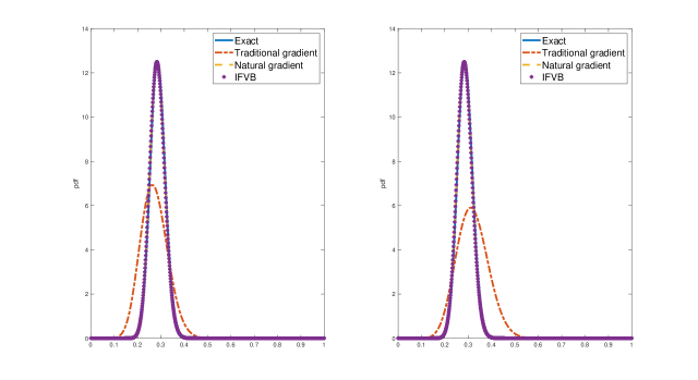
Figure 1. Comparing exact posterior density versus those obtained by gradient ascent, NGVB and IFVB.

As we know the exact posterior distribution in this case, we now further compare the performance of NGVB, IFVB and AIFVB using the initialization $\lambda^{(0)}=(5;45)^{\top}$. Figure 2 plots the error $\left\|\lambda^{(s)}-\lambda^{*}\right\|$ as the function of the number of iterations. It is clear from Figure 2 that both the IFVB and AIFVB algorithms require more steps to achieve a (relatively) equivalent error level compared to the exact natural gradient descent algorithm. This observation aligns with the fact that both algorithms rely on an approximation of the inverse Fisher information matrix. As time advances, the quality of this approximation improves. Furthermore, it is evident that the incorporation of an averaging technique significantly aids in minimizing the error associated with the approximation.

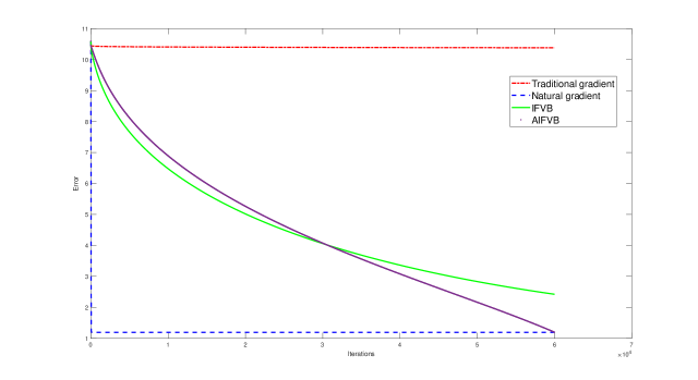
Figure 2. Error versus iterations

Example 2. Let $y=(11;12;8;10;9;8;9;10;13;7)$ be observations from $\mathcal{N}(\mu,\sigma^{2})$, the normal distribution with mean $\mu$ and variance $\sigma^{2}$. We use the prior $\mathcal{N}(\mu_{0},\sigma_{0}^{2})$ for $\mu$ and Inverse-Gamma$(\alpha_{0},\beta_{0})$ for $\sigma^{2}$ with the hyperparameters $\mu_{0}=0,\sigma_{0}=10,\alpha_{0}=1,\beta_{0}=1$. The posterior distribution is written as

$$p(\mu,\sigma^{2}|y)\propto p(\mu)p(\sigma^{2})p(y|\mu,\sigma^{2}).$$

Assume that the VB approximation is $q_{\lambda}(\theta)=q(\mu)q(\sigma^{2})$ with $q(\mu)=\mathcal{N}(\mu_{\mu},\sigma_{\mu}^{2})$, $q(\sigma^{2})=\mbox{Inverse-Gamma}(\alpha_{\sigma^{2}},\beta_{\sigma^{2}})$, model parameter $\theta=(\mu,\sigma^{2})^{\top}$ and the variational parameters $\lambda=(\mu_{\mu},\sigma^{2}_{\mu},\alpha_{\sigma^{2}},\beta_{\sigma^{2}})$. Note that we have $h_{\lambda}(\theta)=h(\theta)-\log q_{\lambda}(\theta)$ with

$$h(\theta) =\log(p(\mu)p(\sigma^{2})p(y|\mu,\sigma^{2}))$$

$$=-\frac{n+1}{2}\log(2\pi)-\frac{1}{2}\log(\sigma_{0}^{2})-\frac{(\mu-\mu_{0})^{2}}{2\sigma_{0}^{2}}+\alpha_{0}\log(\beta_{0})-\log\Gamma(\alpha_{0})$$

$$-(n/2+\alpha_{0}+1)\log(\sigma^{2})-\frac{\beta_{0}}{\sigma^{2}}-\frac{1}{2\sigma^{2}}\sum_{i=1}^{n}(y_{i}-\mu)^{2}.$$

and

$$\log q_{\lambda}(\theta) =\alpha_{\sigma^{2}}\log\beta_{\sigma^{2}}-\log\Gamma(\alpha_{\sigma^{2}})-(\alpha_{\sigma^{2}}+1)\log\sigma^{2}-\frac{\beta_{\sigma^{2}}}{\sigma^{2}}$$

$$-\frac{1}{2}\log(2\pi)-\frac{1}{2}\log(\sigma^{2}_{\mu})-\frac{(\mu-\mu_{\mu})^{2}}{\sigma^{2}_{\mu}}.$$

From here it can be seen that

$$\nabla_{\lambda}\log q_{\lambda}(\theta)=\left(\frac{\mu-\mu_{\mu}}{\sigma^{2}_{\mu}},-\frac{1}{2\sigma^{2}_{\mu}}+\frac{(\mu-\mu_{\mu})^{2}}{2\sigma^{4}_{\mu}},\log\beta_{\sigma^{2}}-\frac{\Gamma^{\prime}(\alpha_{\sigma^{2}})}{\Gamma(\alpha_{\sigma^{2}})}-\log\sigma^{2},\frac{\alpha_{\sigma^{2}}}{\beta_{\sigma^{2}}}-\frac{1}{\sigma^{2}}\right)^{\top}.$$

By direct calculation, it can be seen that the Fisher information matrix $I_{F}$ is a diagonal block matrix with two main blocks

$$\begin{pmatrix}\frac{1}{\sigma^{2}_{\mu}}&0\\ 0&\frac{1}{2\sigma^{4}_{\mu}}\end{pmatrix},\;\;\mbox{ and }\;\;\begin{pmatrix}\frac{\partial^{2}\log\Gamma(\alpha_{\sigma^{2}})}{\partial(\alpha_{\sigma^{2}})^{2}}&-\frac{1}{\beta_{\sigma^{2}}}\\ -\frac{1}{\beta_{\sigma^{2}}}&\frac{\alpha_{\sigma^{2}}}{\beta^{2}_{\sigma^{2}}}\end{pmatrix}.$$

In this example, the natural gradient can be computed in closed-form, which facilitates the testing of our IFVB and AIFVB algorithms. We use $(\overline{y},0.5,1,1)^{\top}$ as the initial guess for $\lambda$. The first and second panel of Figure 3 plot the posterior densities of $\mu$ and $\sigma^{2}$ using all four different approaches: MCMC, exact natural gradient VB (NGVB), inversion free VB (IFVB) and averaged inversion free VB (AIFVB). It can be seen that the posterior estimates obtained by IFVB and AIFVB are close to that of NGVB and MCMC. The last panel of Figure 3 plots the lower bound obtained from the VB methods. As shown, both IFVB and AIFVB converge almost as fast as NGVB even though NGVB uses the exact natural gradient in its computation. We also tried estimate the posterior distribution using the approximated Fisher information $I_{F}$ in (4.1). However, the result is too unstable to report.

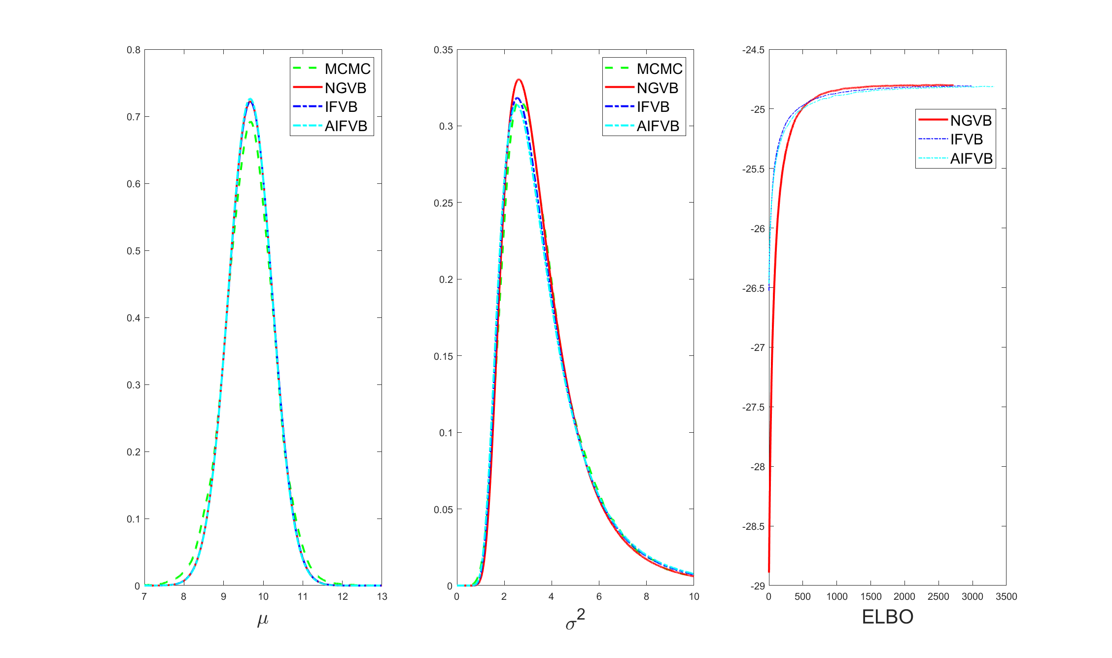
Figure 3. The first two panels show that the IFVB and AIFVB estimates are close to that of the exact natural gradient descent VB (NGVB) and MCMC. The last panel plots the lower bound estimates obtained from NGVB, IFVB and AIFVB.

Example 3. (Gaussian approximation) Assume that $q_{\lambda}(\theta)$ belongs to the exponential family, i.e.,

$$q_{\lambda}(\theta)=c(\theta)\exp\left(s(\theta)^{\top}\lambda-a(\lambda)\right),$$

where $s(\theta)$ is the vector of sufficient statistics, $a(\lambda)$ is the log-partition function, and $c(\theta)$ is a scaling constant. We further assume a minimal exponential family. Recall that $I_{F}=\text{Cov}_{q_{\lambda}}(\nabla_{\lambda}q_{\lambda}(\theta))$. Since $q_{\lambda}(\theta)$ belongs to the exponential family, we have $m:=\mathbb{E}[s(\theta)]=\nabla_{\lambda}a(\lambda)$ and $\text{Cov}(s(\theta))=\nabla_{\lambda}^{2}a(\lambda)=\nabla_{\lambda}m=I_{F}(\lambda)$. Then by the chain rule we have

$$\nabla_{\lambda}\text{\rm LB}(\lambda)=[\nabla_{\lambda}m]\nabla_{m}\text{\rm LB}(m)=\nabla^{2}_{\lambda}a(\lambda)\nabla_{m}\text{\rm LB}(m)=I_{F}(\lambda)\nabla_{m}\text{\rm LB}(m).$$

We note that this fact has been exploited in Hoffman et al. (2013) and Khan and Lin (2017). If we further assume that $q_{\lambda}(\theta)=\mathcal{N}(\theta|\mu,\Sigma)$ which belongs to the exponential family and can be written as

$$q_{\lambda}(\theta)=\exp\left(s(\theta)^{\top}\lambda-a(\lambda)\right),$$

where $s(\theta)=(\theta^{\top},\text{\rm vech}(\theta\theta^{\top})^{\top})^{\top}$ is the sufficient statistics, $\lambda=(\mu^{\top}\Sigma^{-1},-\frac{1}{2}\text{\rm vec}(\Sigma^{-1})^{\top}\Gamma)^{\top}$ is the natural parameter, with $\Gamma$ the duplication matrix. It can be seen that $a(\lambda)=\frac{1}{2}\mu^{\top}\Sigma^{-1}\mu+\frac{1}{2}\log|\Sigma|+\frac{d}{2}\log(2\pi)$ is the log-partition function. This implies the natural gradient

$$\nabla^{nat}_{\lambda}\text{\rm LB}=I^{-1}_{F}(\lambda)\nabla_{\lambda}\text{\rm LB}(\lambda)=I^{-1}_{F}(\lambda)I_{F}(\lambda)\nabla_{m}\text{\rm LB}(m)=\nabla_{m}\text{\rm LB}=\begin{pmatrix}\nabla_{\mu}\text{\rm LB}-2(\nabla_{\Sigma}\text{\rm LB})\mu\\ \Gamma^{\top}\text{\rm vec}(\nabla_{\Sigma}\text{\rm LB})\end{pmatrix},$$

where $\text{\rm vec}(\nabla_{\Sigma}\text{\rm LB})=\nabla_{\text{\rm vec}(\Sigma)}\text{\rm LB}$. From here Tan (2021) derives the updates for $\lambda$ as follows,

1. $\Sigma^{-1}\leftarrow\Sigma^{-1}-2\alpha_{k}\nabla_{\Sigma}\text{\rm LB}$

2. $\mu\leftarrow\mu+\alpha_{k}\Sigma\nabla_{\mu}\text{\rm LB}$.

Obviously, the traditional (Euclidean) gradient ascent is given by

1. $\mu\leftarrow\mu+\alpha_{k}\nabla_{\mu}\text{\rm LB}$

2. $\Sigma\leftarrow\Sigma+\alpha_{k}\nabla_{\Sigma}\text{\rm LB}$.

Let us consider a concrete example: Consider the loglinear model for counts, $y_{i}\sim\text{\rm Poisson}(\delta_{i}),\delta_{i}=\exp(x_{i}^{\top}\theta)$ where $x_{i},\theta\in\mathbb{R}^{d}$ are the vector of covariates and regression coefficients, respectively. Assume the prior of $\theta$ is $p(\theta)\sim\mathcal{N}(0,\sigma_{0}^{2}\mathbb{I}_{d})$. We use a Gaussian $q_{\lambda}(\theta)=\mathcal{N}(\theta|\mu,\Sigma)$ to approximate the true posterior distribution of $\theta$. Let $y=y_{1:n}$ and $X=(x_{1},x_{2},\ldots,x_{n})^{\top}$. For each $i=1,\ldots,n$ let $w_{i}=\exp(x_{i}^{\top}\mu+\frac{1}{2}x_{i}^{\top}\Sigma x_{i})$ and $W={\rm diag}(w_{1},\ldots,w_{n})$. By computing directly, the closed form for the ELBO is,

$$\text{\rm LB}(\lambda)=y^{\top}X\mu-\sum_{i=1}^{n}(w_{i}+\log(y_{i}!))-\frac{\mu^{\top}\mu+Tr(\Sigma)}{2\sigma_{0}^{2}}+\frac{1}{2}\log|\Sigma|+\frac{d}{2}(1-\log(\sigma_{0}^{2})).$$

From here it is immediate to see that $\nabla_{\mu}\text{\rm LB}$, $\nabla_{\Sigma}\text{\rm LB}$, and $\nabla_{\text{\rm vec}(\Sigma)}\text{\rm LB}$ are given by

$$\nabla_{\mu}\text{\rm LB}=X^{\top}(y-w)-\frac{\mu}{\sigma_{0}^{2}},$$

$$\nabla_{\Sigma}\text{\rm LB}=-\frac{1}{2}X^{\top}WX-\frac{1}{2\sigma_{0}^{2}}\mathbb{I}+\frac{1}{2}\Sigma^{-1}$$

$$\nabla_{\text{\rm vec}(\Sigma)}\text{\rm LB}=\frac{1}{2}\text{\rm vec}(\Sigma^{-1}-\frac{1}{\sigma_{0}^{2}}\mathbb{I}-X^{\top}WX).$$

Also we have

$$\log q_{\lambda}(\theta)=-\frac{d}{2}\log(2\pi)-\frac{1}{2}\log|\Sigma|-\frac{1}{2}(\theta-\mu)^{\top}\Sigma^{-1}(\theta-\mu).$$

Hence

$$\nabla_{\lambda}q_{\lambda}(\theta) =(\nabla_{\mu}q_{\lambda}(\theta),\nabla_{\text{\rm vec}(\Sigma)}q_{\lambda}(\theta))$$

$$=\left((\theta-\mu)^{\top}\Sigma^{-1},\text{\rm vec}\left(-\frac{1}{2}\Sigma^{-1}+\frac{1}{2}\Sigma^{-1}(\theta-\mu)(\theta-\mu)^{\top}\Sigma^{-1}\right)^{\top}\right)^{\top}\in\mathbb{R}^{d+d^{2}}.$$

We choose $n=200,d=3,\sigma_{0}^{2}=100,\theta=(1,\ldots,1),x_{ij}\sim\mathcal{N}(0,1),$ and simulate $y_{1},\ldots,y_{200}$ from those parameters. In this case $\lambda\in\mathbb{R}^{12}$ hence $I_{F}\in\mathbb{R}^{12\times 12}$. The initial guesses are $\mu^{(0)}=(0,\ldots,0)^{\top}$ and $\Sigma^{(0)}=10^{-2}\mathbb{I}_{d}$. Moreover, we choose the step size $1/(1000+s)^{0.75}$ and $c_{\beta}=1$. As we know the analytical form of the ELBO in this example, in Figure 4 we plot the graphs of $\text{\rm LB}(\lambda)$ (as a function of the number of iterations) obtained from the exact natural gradient ascent algorithm (NGVB) , inversion free gradient algorithm (IFVB) and weighted inversion free algorithm (AIFVB). It can be seen that the three algorithms have almost identical performance in this case. One striking note is that AIFVB even outperforms (obtaining a larger lower bound values) the exact natural gradient algorithm in this case. It again helps to confirm that the averaging technique does improve the rate of convergence. We note that we tempted to include the ELBO obtained from the gradient descent but its performance is too unstable to include. This phenomenon has been observed in Tan (2021) as the matrix $\Sigma$ obtained from the traditional gradient ascent is usually not positive definite, which results in an unstable performance.

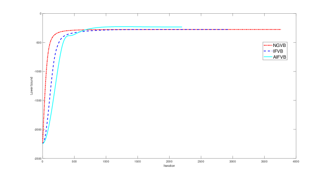
Figure 4. Gaussian Approximation: Comparing NGVB, IFVB and AIFVB

Example 4. (Bayesian neural network) This example considers a Bayesian neural network for regression

(6.1) $$y=\eta(x,\omega)+\epsilon,\;\;\epsilon\sim\mathcal{N}(0,\sigma^{2}),$$

where $y$ is a real-valued response variable, $\eta(x,\omega)$ denotes the output of a neural network with the input vector $x=(x_{1},...,x_{p})^{\top}\in\mathbb{R}^{p}$ and the vector of weights $w$. As neural networks are prone to overfitting, we follow Tran et al. (2020) and place a Bayesian adaptive group Lasso prior on the first-layer weights

(6.2) $$w_{x_{j}}|\tau_{j}\sim\mathcal{N}(0,\tau_{j}\mathbb{I}_{m}),\;\;\;\;\tau_{j}|\gamma_{j}\sim\text{Gamma}\left(\frac{m+1}{2},\frac{\gamma_{j}^{2}}{2}\right),\;\;j=1,...,p,$$

with the $\gamma_{j}>0$ the shrinkage parameters; no regularization prior is put on the rest of the network weights. Here $w_{x_{j}}$ denotes the vector of weights that connect the input $x_{j}$ to the $m$ units in the first hidden layer. An inverse-Gamma prior is used for $\sigma^{2}$. We use empirical Bayes for selecting the shrinkage parameters $\gamma_{j}$, and the posterior of $\tau_{j}$ and $\sigma^{2}$ is approximated by a fixed-form within mean-filed VB procedure. See Tran et al. (2020) for the details.

The main task is to approximate the posterior of the network weights $\omega$. Let $d$ be the dimension of $\omega$. We choose to approximate this posterior by a Gaussian variational distribution of the form $q_{\lambda}(\omega)=\mathcal{N}(\mu,\Sigma)$ with covariance matrix $\Sigma$ having a factor form $\Sigma=bb^{\top}+{\rm diag}(c)^{2}$, where $b$ and $c$ are vectors in $\mathbb{R}^{d}$. The vector of the variational parameters is $\lambda=(\mu^{\top},b^{\top},c^{\top})^{\top}$. This factor structure of the covariance matrix significantly reduces the size of variational parameters, making the Gaussian variational approximation method computationally efficient for Bayesian inference in large models such as Bayesian neural networks.

Tran et al. (2020) exploit the factor structure of $\Sigma$, and by setting certain sub-blocks of the Fisher information matrix $I_{F}(\lambda)$ to zero, to be able to derive a closed-form approximation of the inverse $I_{F}^{-1}(\lambda)$. Their VB method, termed the Natural gradient Gaussian Variational Approximation with factor Covariance method (NAGVAC), is highly computationally efficient; however, the approximation of $I_{F}^{-1}(\lambda)$ might offset the VB approximation accuracy.

We now fit the Bayesian neural network model (6.1) to the the Direct Marketing dataset (Jank, 2011) that consists of 1000 observations, of which 800 were used for training, 100 for validation and the rest for testing. The response $y$ is the amount (in $1000) a customer spends on the company’s products per year, and 11 covariates include gender, income, married status, etc. We use a neural network with two hidden layers, each with ten units. Figure 5 plots the mean squared error (MSE) values, computed on the validation set, of the VB training using NAGVAC, IFVB and AIFVB. With the same stopping rule, the AIFVB and IFVB method stops after 221 and 480 iterations, respectively, while NAGVAC requires almost 700 iterations. This confirms the theoretical result in Theorem 5.3 that the averaging technique speeds up the convergence of AIFVB. On the validation set, the smallest MSE values produced by NAGVAC, IFVB and AIFVB are 0.1992, 0.1749 and 0.1750, respectively. On the test set, the smallest MSE values produced by NAGVAC and IFVB and AIFVB are 0.3469, 0.3031 and 0.3031, respectively. Both IFVB and AIFVB perform better than NAGVAC, probably because the natural gradient approximation in NAGVAC, although being highly computationally efficient, might offset the approximation accuracy.

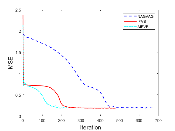
Figure 5. Bayesian neural network: Validation MSE values of NAGVAC (dash blue) versus IFVB (red solid) and AIFVB (dot greenish) over the iterations

Example 5. (Normalizing flow Variational Bayes) The choice of flexible variational distributions $q_{\lambda}$ is important in VB. Normalizing flows (Rezende and Mohamed, 2015) are a class of techniques for designing flexible and expressive $q_{\lambda}$. We consider a flexible VB framework where the VB approximation distribution $q_{\lambda}(\theta)$ is constructed based on a normalizing flow as follows

(6.3) $$\epsilon\sim\mathcal{N}_{d}(0,I),\;\;Z=h(W_{1}\epsilon+b_{1}),\;\;\theta=W_{2}Z+b_{2}$$

where $W_{1},W_{2}\in\text{Mat}(d,d)$ and $b_{1},b_{2}$ are $d$-vectors, and $h(\cdot)$ is an activation function such as sigmoid. The transformation from $\epsilon$ to $\theta$ in (6.3) can be viewed as a neural network with one hidden layer $Z$; it might be desirable to consider deeper neural nets with more than one hidden layers, but we do not consider it here. To be able to compute the density $q_{\lambda}(\theta)$ resulting from the transformations in (6.3), these transformations should be invertibe and the determinants of the Jacobian matrices should be easy to compute. To this end, we impose the orthogonality constraint on $W_{1}$ and $W_{2}$: $W_{1}^{\top}W_{1}=W_{2}^{\top}W_{2}=\mathbb{I}_{d}$, i.e. the columns are orthonormal. Details on the derivation of the lower bound gradient and score function $\nabla\log q_{\lambda}(\theta)$ can be found in Appendix E.

Numerical results

We apply the manifold normalizing flow VB (NLVB) (6.3) to approximate the posterior distribution in a neural network classification problem, using the German Credit dataset. This dataset, available on the UCI Machine Learning Repository https://archive.ics.uci.edu/ml/index.php, consists of observations on 1000 customers, each was already rated as being “good credit” (700 cases) or “bad credit” (300 cases). We create 10 predictors out of the available covariate variables including credit history, education, employment status, etc. The classification problem is based on a neural network with one hidden layer of 5 units. As $W_{1}$ and $W_{2}$ belong to the Stiefel manifold, for a comparison we use the VB on manifold algorithm of Tran et al. (2021) for updating these parameters. Figure 6 plots the lower bounds of the IFVB algorithm (solid red) together with the conventional VB algorithm (dash blue) using the ordinary gradient (E.1) in the Appendix. As shown, the IFVB algorithm converges quicker and achieves a higher lower bound. Note that we do not consider the AIFVB algorithm in this example, as the variational parameters belong to the Stiefel manifold, making the averaging technique more challenging. It is interesting to extend the work to handle cases where the parameter space is a Riemannian manifold; however, we do not consider this in the present paper.

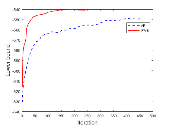
Figure 6. Normalizing flow VB: Lower bound values of ordinary gradient VB (dash blue) versus IFVB (solid red) over the iterations.

7. Conclusion

The paper introduced an efficient approach for approximating the inverse of Fisher information, a crucial component in variational Bayes used for approximating posterior distributions. An outstanding feature of our algorithm is its avoidance of explicit matrix inversion. Instead, our approach generates a sequence of matrices converging to the inverse of Fisher information. Our inversion free VB framework showcases versatility, enabling its application in a wide range of domains, including Gaussian approximation and normalizing flow Variational Bayes, and makes the natural gradient VB method applicable in cases that were impossible before. To demonstrate the efficiency and reliability of the method, we provided numerical examples as evidence of its effectiveness. We find it intriguing to consider expanding the scope of our approach to scenarios where the variational parameter space is a Riemannian manifold and to develop a rigorous theoretical framework for such cases. We plan to explore this avenue in our future research studies.

8. Main proofs

Let us recall that $\alpha_{k}=\frac{c_{\alpha}}{\left(c_{\alpha}^{\prime}+k\right)^{\alpha}}$ with $c_{\alpha}>0$, $c_{\alpha}^{\prime}\geq 0$ and $\alpha\in(1/2,1)$. In addition, $\beta_{k}=\frac{c_{\beta}}{k^{\beta}}$ with $c_{\beta}\geq 0$ and $\beta\in(0,\alpha-1/2)$. Recall that

$$\nabla_{\lambda}\mathcal{L}(\lambda)=\mathbb{E}_{q_{\lambda}}[-\nabla_{\lambda}\log q_{\lambda}(\theta)h_{\lambda}(\theta)]=:\mathbb{E}_{q_{\lambda}}[\ell(\theta,\lambda)].$$

We then have the recursive scheme

$$\lambda^{(k+1)}-\lambda^{(k)}=-\alpha_{k+1}\tilde{\mathbf{H}}^{-1}_{k+1}\frac{1}{B}\sum_{i=1}^{B}\ell(\theta_{k+1,i},\lambda^{(k)}),\;\;\;\theta_{k+1,i}\sim q_{\lambda^{(k)}}(\theta).$$

8.1. Proof of Theorem 5.1

Proof.

From Taylor’s expansion of $\mathcal{L}(\lambda)$, since its Hessian is uniformly bounded, we have

$$\mathcal{L}(\lambda^{(k+1)})=\mathcal{L}(\lambda^{(k)})+\nabla_{\lambda}\mathcal{L}^{\top}(\lambda^{(k)})(\lambda^{(k+1)}-\lambda^{(k)})$$

$$+(\lambda^{(k+1)}-\lambda^{(k)})^{\top}\Big{(}\int_{0}^{1}(1-t)\nabla_{\lambda}^{2}\mathcal{L}(\lambda^{(k+1)}+t(\lambda^{(k)}-\lambda^{(k+1)}))dt\Big{)}(\lambda^{(k+1)}-\lambda^{(k)})$$

$$\leq\mathcal{L}(\lambda^{(k)})+\nabla_{\lambda}\mathcal{L}^{\top}(\lambda^{(k)})(\lambda^{(k+1)}-\lambda^{(k)})+\frac{1}{2}L_{0}\left\|(\lambda^{(k+1)}-\lambda^{(k)})\right\|^{2}$$

$$\leq\mathcal{L}(\lambda^{(k)})-\alpha_{k+1}\nabla_{\lambda}\mathcal{L}^{\top}(\lambda^{(k)})\tilde{\mathbf{H}}^{-1}_{k+1}\frac{1}{B}\sum_{i=1}^{B}\ell(\theta_{k+1,i},\lambda^{(k)})$$

$$\phantom{cccc}+\frac{1}{2B}\alpha_{k+1}^{2}L_{0}\left\|\tilde{\mathbf{H}}^{-1}_{k+1}\right\|_{op}^{2}\sum_{i=1}^{B}\left\|\ell(\theta_{k+1,i},\lambda^{(k)})\right\|^{2}$$

Hence

$$\mathcal{L}(\lambda^{(k+1)})-\mathcal{L}(\lambda^{*}) \leq\mathcal{L}(\lambda^{(k)})-\mathcal{L}(\lambda^{*})-\alpha_{k+1}\nabla_{\lambda}\mathcal{L}^{\top}(\lambda^{(k)})\tilde{\mathbf{H}}^{-1}_{k+1}\frac{1}{B}\sum_{i=1}^{B}\ell(\theta_{k+1,i},\lambda^{(k)})$$

$$+\frac{1}{2B}\alpha_{k+1}^{2}L_{0}\left\|\tilde{\mathbf{H}}^{-1}_{k+1}\right\|_{op}^{2}\sum_{i=1}^{B}\left\|\ell(\theta_{k+1,i},\lambda^{(k)})\right\|^{2}.$$

Let us denote $W_{k}=\mathcal{L}(\lambda^{(k)})-\mathcal{L}(\lambda^{*})$. From the above inequality we have

$$W_{k+1}\leq W_{k}-\alpha_{k+1}\nabla_{\lambda}\mathcal{L}^{\top}(\lambda^{(k)})\tilde{\mathbf{H}}^{-1}_{k+1}\frac{1}{B}\sum_{i=1}^{B}\ell(\theta_{k+1,i},\lambda^{(k)})$$

$$+\frac{1}{2B}\alpha_{k+1}^{2}L_{0}\left\|\tilde{\mathbf{H}}^{-1}_{k+1}\right\|_{op}^{2}\sum_{i=1}^{B}\left\|\ell(\theta_{k+1,i},\lambda^{(k)})\right\|^{2}.$$

Let us consider the filtration $\mathcal{F}_{k}=\sigma(\theta_{s,i},\overline{\theta}_{s^{\prime}},Z_{s}:s\leq k:s^{\prime}\leq k+1)$. As $\theta_{k+1,i}$ are independent of $\mathcal{F}_{k}$, taking the conditional expectation from the both sides of the above inequality, we have

$$\mathbb{E}[W_{k+1}|\mathcal{F}_{k}] \leq\mathbb{E}[W_{k}|\mathcal{F}_{k}]-\alpha_{k+1}\frac{1}{B}\sum_{i=1}^{B}\mathbb{E}[\nabla_{\lambda}\mathcal{L}^{\top}(\lambda^{(k)})\tilde{\mathbf{H}}^{-1}_{k+1}\ell(\theta_{k+1,i},\lambda^{(k)})|\mathcal{F}_{k}]$$

$$\phantom{cccc}+\frac{1}{2B}\alpha_{k+1}^{2}L_{0}\sum_{i=1}^{B}\left\|\tilde{\mathbf{H}}^{-1}_{k+1}\right\|_{op}^{2}\mathbb{E}[\left\|\ell(\theta_{k+1,i},\lambda^{(k)})\right\|^{2}|\mathcal{F}_{k}]$$

$$\leq W_{k}-\alpha_{k+1}\nabla_{\lambda}\mathcal{L}^{\top}(\lambda^{(k)})\tilde{\mathbf{H}}^{-1}_{k+1}\nabla_{\lambda}\mathcal{L}(\lambda^{(k)})$$

$$\phantom{cccc}+\frac{1}{2B}\alpha_{k+1}^{2}L_{0}\left\|\tilde{\mathbf{H}}^{-1}_{k+1}\right\|_{op}^{2}\sum_{i=1}^{B}\mathbb{E}\left[\left\|\ell(\theta_{k+1,i},\lambda^{(k)})\right\|^{2}|\mathcal{F}_{k}\right].$$

Since $\mathbb{E}[\left\|\ell(\theta,\lambda)\right\|^{2}]\leq C_{0}+C_{1}(\mathcal{L}(\lambda)-\mathcal{L}(\lambda^{*}))$, we have

$$\mathbb{E}[W_{k+1}|\mathcal{F}_{k}] \leq\left(1+\frac{C_{1}L_{0}}{2}\alpha_{k+1}^{2}\left\|\tilde{\mathbf{H}}^{-1}_{k+1}\right\|_{op}^{2}\right)W_{k}-\alpha_{k+1}\lambda_{min}(\tilde{\mathbf{H}}^{-1}_{k+1})\left\|\nabla_{\lambda}\mathcal{L}(\lambda^{(k)})\right\|^{2}$$

$$+\frac{1}{2}\alpha_{k+1}^{2}C_{0}L_{0}\left\|\tilde{\mathbf{H}}^{-1}_{k+1}\right\|_{op}^{2}.$$

In order to apply the Robbins-Siegmund theorem (Robbins and Siegmund, 1971), we now focus on the behavior of the eigenvalues of $\tilde{\mathbf{H}}_{s}$. Observe that with the help of Toeplitz lemma (e.g., see the proof of Theorem B.1 in Appendix B).

$$(1-\beta)s^{1-\beta}\sum_{k=1}^{s}k^{-\beta}Z_{k}Z_{k}^{\top}\xrightarrow[s\to+\infty]{}I.$$

Then, as soon as $\lambda_{\min}\left(\tilde{\mathbf{H}}_{s}\right)\geq\lambda_{\min}\left(\frac{1}{s}H_{0}+\frac{1}{s}\sum_{k=1}^{s}c_{\beta}k^{-\beta}Z_{k}Z_{k}^{\top}\right)$, it comes

$$\lambda_{\max}\left(\tilde{\mathbf{H}}_{s}^{-1}\right)=O\left(s^{\beta}\right)\quad a.s.$$

Then, since $\beta<\alpha-1/2$, i.e $2\alpha-2\beta>1$, it comes

$$\sum_{k}\alpha_{k+1}^{2}\left\|\tilde{\mathbf{H}}_{k+1}^{-1}\right\|^{2}\leq C\sum_{k}k^{2\beta-2\alpha}<+\infty\quad a.s.$$

Using the Robbins-Siegmund theorem, one has that $W_{k}$ converges almost surely to a random variable $W_{\infty}$ and that

(8.1) $$\sum_{k=0}^{\infty}\alpha_{k+1}\lambda_{\min}(\tilde{\mathbf{H}}^{-1}_{k+1})\left\|\nabla\mathcal{L}\left(\lambda^{(k)}\right)\right\|^{2}<\infty,\quad\mbox{a.s}.$$

We now have to control the smallest eigenvalue of $\tilde{\mathbf{H}}^{-1}_{s+1}$. In this aim, let us remark that the estimates of the Fisher Information can be written as

$$\tilde{\mathbf{H}}_{s}=\frac{1}{s}\left(H_{0}+\sum_{k=1}^{s}\beta_{k}Z_{k}Z_{k}^{T}\right) +\underbrace{\frac{1}{s}\sum_{k=0}^{s-1}\mathbb{E}\left[\nabla_{\lambda}\log q_{\overline{\lambda}^{(k)}}(\overline{\theta}_{k+1})\nabla_{\lambda}\log q_{\overline{\lambda}^{(k)}}(\overline{\theta}_{k+1})^{\top}|\tilde{\mathcal{F}}_{k}\right]}_{=:R_{s}}$$

$$+\underbrace{\frac{1}{s}\sum_{k=0}^{s-1}\Xi_{k+1}}_{=:M_{s}},$$

where $\tilde{\mathcal{F}}_{k}=\sigma\left(\theta_{s,i},\overline{\theta}_{s},Z_{s}:s\leq k,i\leq B\right)$ and

$$\Xi_{k+1}:=-\mathbb{E}\left[\nabla_{\lambda}\log q_{\overline{\lambda}^{(k)}}(\overline{\theta}_{k+1})\nabla_{\lambda}\log q_{\overline{\lambda}^{(k)}}(\overline{\theta}_{k+1})^{\top}|\tilde{\mathcal{F}}_{k}\right]+\nabla_{\lambda}\log q_{\overline{\lambda}^{(k)}}(\overline{\theta}_{k+1})\nabla_{\lambda}\log q_{\overline{\lambda}^{(k)}}(\overline{\theta}_{k+1})^{\top}$$

is a sequence of martingale differences. In addition

(8.2) $$\mathbb{E}\left[\left\|M_{s+1}\right\|_{F}^{2}|\mathcal{F}_{s}\right] \leq\left(\frac{s}{s+1}\right)^{2}\left\|M_{s}\right\|_{F}^{2}+\frac{1}{(s+1)^{2}}\mathbb{E}\left[\left\|\nabla_{\lambda}\log q_{\overline{\lambda}^{(k)}}(\overline{\theta}_{k+1})\right\|^{4}|\tilde{\mathcal{F}}_{s}\right].$$

and since there are positive constants $C_{0}^{\prime},C_{1}^{\prime}$ such that for all $\lambda$,

$$\mathbb{E}\left[\left\|\nabla_{\lambda}\log q_{\lambda}(\theta)\right\|^{4}\right]\leq C_{0}^{\prime}+C_{1}^{\prime}\left(\mathcal{L}(\lambda)-\mathcal{L}\left(\lambda^{*}\right)\right)^{2},$$

observe that $\mathbb{E}\left[\left\|\nabla_{\lambda}\log q_{\overline{\lambda}^{(k)}}(\overline{\theta}_{k+1})\right\|^{4}|\tilde{\mathcal{F}}_{k}\right]\leq C_{0}^{\prime}+C_{1}^{\prime}\overline{W}_{k}^{2}$ where $\overline{W}_{k}=\mathcal{L}\left(\overline{\lambda}^{(k)}\right)-\mathcal{L}\left(\lambda^{*}\right)$. By the convexity of $\mathcal{L}$ and with the help of the Toeplitz lemma,

$$\overline{W}_{s}\leq\frac{1}{\sum_{k=0}^{s}\log(k+1)^{w}}\sum_{k=0}^{s}\log(k+1)^{w}\left(\mathcal{L}\left(\lambda^{(k)}\right)-\mathcal{L}\left(\lambda^{*}\right)\right)\xrightarrow[n\to+\infty]{a.s}W_{\infty}.$$

Then, from (8.2), applying the Robbins-Siegmund theorem, $\left\|M_{s}\right\|_{F}^{2}=\mathcal{O}(1)$ a.s. In a same way, one can check that $\left\|R_{s}\right\|_{F}^{2}=\mathcal{O}(1)$ a.s. This means that at least,

$$\liminf_{k}\lambda_{\min}\left(\tilde{\mathbf{H}}_{k}^{-1}\right)>0$$

i.e. that $\sum_{k=0}^{\infty}\alpha_{k+1}\lambda_{\min}(\tilde{\mathbf{H}}^{-1}_{k+1})=+\infty$. It implies from (8.1) that $\liminf_{k}\left\|\nabla\mathcal{L}\left(\lambda^{(k)}\right)\right\|^{2}>0$ a.s., and one can conclude thanks to the strict convexity of $\mathcal{L}$ that $W_{k}$ converges almost surely to $W_{\infty}=0$. Hence $\mathcal{L}(\lambda^{(k)}\rightarrow\mathcal{L}(\lambda^{*})$ almost surely. Therefore, $\lambda^{(k)}\rightarrow\lambda^{*}$ almost surely.

This completes the proof of the theorem.

∎

8.2. Proof of Corollary 5.1

Proof.

Let us recall from the proof of Theorem 5.1 that $\tilde{\mathbf{H}}_{s}=\frac{1}{s}\left(H_{0}+\sum_{k=1}^{s}\beta_{k}Z_{k}Z_{k}^{T}\right)+R_{s}+M_{s}$. Similar to the proof of Theorem B.1 in Appendix B, the norm of the first term can be estimated as

$$\left\|\frac{1}{s}\left(H_{0}+\sum_{k=0}^{s-1}\beta_{k}Z_{k}Z_{k}^{T}\right)\right\|=\mathcal{O}\left(\max\left\{c_{\beta}s^{-\beta},s^{-1}\right\}\right)\quad a.s.$$

which is is negligible. By the continuity of $I_{F}(\lambda)$ and since the convergence of $\lambda^{(k)}$ implies that $\overline{\lambda}^{(k)}$ converges almost surely to $\lambda^{*}$, it comes

$$R_{s}=\frac{1}{s}\sum_{k=0}^{s}\mathbb{E}\left[\nabla_{\lambda}\log q_{\overline{\lambda}^{(k)}}(\overline{\theta}_{k+1})\nabla_{\lambda}\log q_{\overline{\lambda}^{(k)}}(\overline{\theta}_{k+1})^{\top}|\tilde{\mathcal{F}}_{k}\right]\xrightarrow[n\to+\infty]{a.s}I_{F}\left(\lambda^{*}\right).$$

Finally, applying Theorem 6.2 in Cénac et al. (2020), it comes that for any $\delta>0$,

$$\left\|M_{s}\right\|_{F}^{2}=o\left(\frac{\log s^{1+\delta}}{s}\right)\quad a.s.$$

which is negligible. ∎

8.3. Proof of Theorem 5.2

Proof.

The proof is adapted from Boyer and Godichon-Baggioni (2023) and Bercu et al. (2020). Denoting $I_{F}=I_{F}\left(\lambda^{*}\right)$,

$$\lambda^{(k+1)}-\lambda^{*}=\lambda^{(k)}-\lambda^{*}-\alpha_{k+1}\tilde{\mathbf{H}}_{k+1}^{-1}\frac{1}{B}\sum_{i=1}^{B}\ell(\theta_{k+1,i},\lambda^{(k)})$$

$$=\lambda^{(k)}-\lambda^{*}-\alpha_{k+1}\tilde{\mathbf{H}}_{k+1}^{-1}\nabla_{\lambda}\mathcal{L}(\lambda^{(k)})+\alpha_{k+1}\tilde{\mathbf{H}}_{k+1}^{-1}\underbrace{\left(\nabla_{\lambda}\mathcal{L}(\lambda^{(k)})-\frac{1}{B}\sum_{i=1}^{B}\ell(\theta_{k+1,i},\lambda^{(k)})\right)}_{\xi_{k+1}}$$

$$=\lambda^{(k)}-\lambda^{*}-\alpha_{k+1}I^{-1}_{F}\nabla_{\lambda}\mathcal{L}(\lambda^{(k)})-\alpha_{k+1}\underbrace{\left(\tilde{\mathbf{H}}_{k+1}^{-1}-I^{-1}_{F}\right)\nabla_{\lambda}\mathcal{L}(\lambda^{(k)})}_{=:r_{k}}+\alpha_{k+1}\tilde{\mathbf{H}}_{k+1}^{-1}\xi_{k+1}$$

$$=\left(\mathbb{I}-\alpha_{k+1}I^{-1}_{F}\nabla^{2}\mathcal{L}\left(\lambda^{*}\right)\right)\left(\lambda^{(k)}-\lambda^{*}\right)-\alpha_{k+1}r_{k}+\alpha_{k+1}\tilde{\mathbf{H}}_{k+1}^{-1}\xi_{k+1}$$

(8.3) $$\phantom{cccc}-\alpha_{k+1}I_{F}^{-1}\underbrace{\left(\nabla\mathcal{L}\left(\lambda^{(k)}\right)-\nabla^{2}\mathcal{L}\left(\lambda^{*}\right)\left(\lambda^{(k)}-\lambda^{*}\right)\right)}_{=:\delta_{k}}$$

As explained in Antonakopoulos et al. (2022), since $I_{F}$ and $\nabla^{2}\mathcal{L}\left(\lambda^{*}\right)$ are symmetric and positive, $I^{-1}_{F}\nabla^{2}\mathcal{L}\left(\lambda^{*}\right)$ and $I^{-1/2}_{F}\nabla^{2}\mathcal{L}\left(\lambda^{*}\right)I^{-1/2}_{F}$ have the same eigenvalues, i.e there is a positive diagonal matrix $\Lambda$ (of the eigenvalues of $I^{-1/2}_{F}\nabla^{2}\mathcal{L}\left(\lambda^{*}\right)I^{-1/2}_{F}$) and a matrix $Q$ such that $I^{-1}_{F}\nabla^{2}\mathcal{L}\left(\lambda^{*}\right)=Q^{-1}\Lambda Q$. Then one can rewrite the previous decomposition as

(8.4) $$Q\left(\lambda^{(k+1)}-\lambda^{*}\right)=\left(I-\alpha_{k+1}\Lambda\right)Q\left(\lambda^{(k)}-\lambda^{*}\right)-\alpha_{k+1}Qr_{k}+\alpha_{k+1}Q\tilde{\mathbf{H}}_{k+1}^{-1}\xi_{k+1}-\alpha_{k+1}QI_{F}^{-1}\delta_{k}.$$

Then, with the help of an induction, it comes that

$$Q\left(\lambda^{(s)}-\lambda^{*}\right) =\beta_{s,0}Q\left(\lambda^{(0)}-\lambda^{*}\right)+\underbrace{\sum_{k=0}^{s-1}\beta_{s,k+1}\alpha_{k+1}Q\tilde{\mathbf{H}}_{k+1}^{-1}\xi_{k+1}}_{=:M_{s}^{\prime}}$$

(8.5) $$-\underbrace{\left(\sum_{k=0}^{s-1}\beta_{s,k+1}\alpha_{k+1}Qr_{k}+\sum_{k=0}^{s-1}\beta_{s,k+1}\alpha_{k+1}QI_{F}^{-1}\delta_{k}\right)}_{\Delta_{s}}.$$

with $\beta_{s,k}=\prod_{j=k+1}^{s}\left(\mathbb{I}-\alpha_{j}\Lambda\right)$ and $\beta_{s,s}=\mathbb{I}$. We now give the rate of convergence for each term in the decomposition (8.3).

Rate of convergence of $\beta_{s,0}Q\left(\lambda^{(0)}-\lambda^{*}\right)$. Since $\lambda_{\min}(\Lambda)>0$ (because $I_{F}$ and $\nabla^{2}\mathcal{L}\left(\lambda^{*}\right)$ are positive), one can easily check that

$$\left\|\beta_{s,0}Q\left(\lambda^{(0)}-\lambda^{*}\right)\right\|=\mathcal{O}\left(\exp\left(-\lambda_{\min}(\Lambda)\frac{c_{\alpha}}{1-\alpha}s^{1-\alpha}\right)\right)\quad a.s.$$

Rate of convergence of $M_{s}^{\prime}$. Recall there are $\eta>\frac{1}{\alpha}-1$ and positive constants $C_{\eta,0},C_{\eta,1}$ such that for all $\lambda$,

$$\mathbb{E}\left[\left\|l(\theta,\lambda)\right\|^{2+2\eta}\right]\leq C_{\eta,0}+C_{\eta,1}\left(\mathcal{L}(\lambda)-\mathcal{L}\left(\lambda^{*}\right)\right)^{1+\eta}.$$

Then, one has with the help of Hölder’s inequality

$$\mathbb{E}\left[\left\|\xi_{k+1}\right\|^{2+2\eta}|\mathcal{F}_{k}\right] \leq 2^{2\eta+1}\frac{1}{B}\sum_{i=1}^{B}\mathbb{E}\left[\left\|\ell\left(\theta_{k+1,i},\lambda^{(k)}\right)\right\|^{2+2\eta}|\mathcal{F}_{k}\right]+2^{2\eta+1}\left\|\nabla_{\lambda}\mathcal{L}\left(\lambda^{(k)}\right)\right\|^{2+2\eta}$$

$$\leq 2^{2+2\eta}C_{\eta,0}+2^{2+2\eta}C_{\eta,1}\left(\mathcal{L}\left(\overline{\lambda}^{(k)}\right)-\mathcal{L}\left(\lambda^{*}\right)\right)^{1+\eta}.$$

Since $\lambda^{(k)}$ is strongly consistent, the second term on the right-hand side of previous inequality converges almost surely to $0$. In addition, thanks to Corollary 5.1, $\tilde{\mathbf{H}}_{k}^{-1}$ converges almost surely to $I_{F}^{-1}$. Then, with the help of Theorem 6.1 in Cénac et al. (2020),

$$\left\|M_{s}^{\prime}\right\|^{2}=\mathcal{O}\left(\frac{\log s}{s^{\alpha}}\right)\quad a.s.$$

Rate of convergence of $\Delta_{s}$. For $s$ large enough, one has

$$\left\|\Delta_{s+1}\right\|\leq\left(1-\lambda_{\min}(\Lambda)\alpha_{s+1}\right)\left\|\Delta_{s}\right\|+\alpha_{s+1}\left\|Q\right\|\left(\left\|r_{s}\right\|+\left\|I_{F}^{-1}\right\|\left\|\delta_{s}\right\|\right).$$

Observe that since $\mathcal{L}$ is twice continuously differentiable on a neighborhood of $\lambda^{*}$ and since $\lambda^{(k)}$ is strongly consistent, it comes that $\left\|\delta_{k}\right\|=o\left(\left\|\lambda^{(k)}-\lambda^{*}\right\|\right)$ a.s. In addition, since $\tilde{\mathbf{H}}_{k}^{-1}$ converges almost surely to $I_{F}^{-1}$ and since the gradient of $\mathcal{L}$ is locally Lipschitz on a neighborhood of $\lambda^{*}$ (since the Hessian is locally bounded by continuity), one has that $\|r_{k}\|=o\left(\left\|\lambda^{(s)}-\lambda^{*}\right\|\right)$ a.s. Then, $\left\|r_{s}\right\|+\left\|I_{F}^{-1}\right\|\left\|\delta_{s}\right\|=o\left(\left\|\lambda^{(s)}-\lambda^{*}\right\|\right)$ a.s, and with the help of decompotision (8.3), it comes that

$$\left\|r_{s}\right\|+\left\|I_{F}^{-1}\right\|\left\|\delta_{s}\right\|=o\left(\left\|\beta_{s,0}Q\left(\lambda^{(0)}-\lambda^{*}\right)\right\|+\left\|M_{s}^{\prime}\right\|+\left\|\Delta_{s}\right\|\right)\quad a.s.$$

Thanks to previous convergence results, there exists a sequence of random variables $r_{s}^{\prime}$ converging almost surely to $0$ such that

$$\left\|\Delta_{s+1}\right\|\leq\left(1-\lambda_{\min}(\Lambda)\alpha_{s+1}\right)\left\|\Delta_{s}\right\|+\alpha_{s+1}r_{s+1}\left(\sqrt{\frac{\log s}{s^{\alpha}}}+\left\|\Delta_{s}\right\|\right).$$

Then, thanks to a stabilization Lemma (see Duflo (2013)), it comes

$$\left\|\Delta_{s}\right\|=\mathcal{O}\left(\sqrt{\frac{\log s}{s^{\alpha}}}\right)\quad a.s,$$

which concludes the proof. ∎

8.4. Proof of Theorem 5.3

Proof.

Observe that one can rewrite decomposition (8.3) as

$$\lambda^{(k+1)}-\lambda^{*} =\lambda^{(k)}-\lambda^{*}-\alpha_{k+1}\tilde{\mathbf{H}}_{k+1}^{-1}\nabla_{\lambda}\mathcal{L}\left(\lambda^{(k)}\right)+\alpha_{k+1}\tilde{\mathbf{H}}_{k+1}^{-1}\xi_{k+1}$$

$$=\lambda^{(k)}-\lambda^{*}-\alpha_{k+1}\tilde{\mathbf{H}}_{k+1}^{-1}\nabla_{\lambda}^{2}\mathcal{L}(\lambda^{*})\left(\lambda^{(k)}-\lambda^{*}\right)-\alpha_{k+1}\tilde{\mathbf{H}}_{k+1}^{-1}\delta_{k}+\alpha_{k+1}\tilde{\mathbf{H}}_{k+1}^{-1}\xi_{k+1},$$

where $\delta_{k}=\nabla\mathcal{L}\left(\lambda^{(k)}\right)-\nabla^{2}\mathcal{L}\left(\lambda^{*}\right)\left(\lambda^{(k)}-\lambda^{*}\right)$ and $\xi_{k+1}=\nabla_{\lambda}\mathcal{L}(\lambda^{(k)})-\frac{1}{B}\sum_{i=1}^{B}\ell(\theta_{k+1,i},\lambda^{(k)})$. Denoting $u_{k}:=\lambda^{(k)}-\lambda^{*}$ and $L^{-1}:=\nabla_{\lambda}^{2}\mathcal{L}(\lambda^{*})^{-1}$, one can rewrite

$$\lambda^{(k)}-\lambda^{*}=L^{-1}\tilde{\mathbf{H}}_{k+1}^{-1}\frac{u_{k}-u_{k+1}}{\alpha_{k+1}}+L^{-1}\xi_{k+1}-L^{-1}\delta_{k}.$$

Multiplying by $\log(k+1)^{w}$, then summing these equalities and dividing by $\sum_{k=0}^{s}\log(k+1)^{w}$, it comes

$$\overline{\lambda}^{(s)}-\lambda^{*} =L^{-1}\underbrace{\frac{1}{\sum_{k=0}^{s}\log(k+1)^{w}}\sum_{k=0}^{s}\log(k+1)^{w}\tilde{\mathbf{H}}_{k+1}^{-1}\frac{u_{k}-u_{k+1}}{\alpha_{k+1}}}_{=:A_{1,s}}$$

$$-L^{-1}\underbrace{\frac{1}{\sum_{k=0}^{s}\log(k+1)^{w}}\sum_{k=0}^{s}\log(k+1)^{w}\delta_{k}}_{A_{2,s}}+\underbrace{\frac{L^{-1}}{\sum_{k=0}^{s}\log(k+1)^{w}}\sum_{k=0}^{s}\log(k+1)^{w}\xi_{k+1}}_{M_{2,s}}.$$

The aim is to give the rate of convergence for each term on the right-hand side of the decomposition above. Let us first denote $t_{s}=\sum_{k=0}^{s}\log(k+1)^{w}$ and observe that

(8.6) $$\ t_{s}\sim s\log(s+1)^{w}.$$

Rate of convergence of $\mathbf{A_{1,s}}$. First, note that

$$A_{1,s}=\frac{1}{t_{s}}\sum_{k=0}^{s}\log(k+1)^{w}\frac{\tilde{\mathbf{H}}_{k}^{-1}u_{k}-\tilde{\mathbf{H}}_{k+1}^{-1}u_{k+1}}{\alpha_{k+1}}+\frac{1}{t_{s}}\sum_{k=0}^{s}\log(k+1)^{w}\left(\tilde{\mathbf{H}}_{k+1}^{-1}-\tilde{\mathbf{H}}_{k}^{-1}\right)\frac{u_{k}}{\alpha_{k+1}}.$$

Concerning the first term on the right hand-side of previous equality, with the help of Abel’s transform,

$$\frac{1}{t_{s}}\sum_{k=0}^{s}\log(k+1)^{w}\frac{\tilde{\mathbf{H}}_{k}^{-1}u_{k}-\tilde{\mathbf{H}}_{k+1}^{-1}u_{k+1}}{\alpha_{k+1}} =-\frac{\log(s+1)^{w}\tilde{\mathbf{H}}_{s+1}^{-1}u_{s+1}}{t_{s}\alpha_{s+1}}+\frac{\mathbf{1}_{w=0}\tilde{\mathbf{H}}_{0}^{-1}u_{0}}{t_{s}\alpha_{1}}$$

$$+\sum_{k=1}^{s}\tilde{\mathbf{H}}_{k}^{-1}u_{k}\left(\frac{\log(k+1)^{w}}{\alpha_{k+1}}-\frac{\log(k)^{w}}{\alpha_{k}}\right).$$

With the help of an Abel’s transform, one has

$$\frac{1}{t_{s}}\sum_{k=0}^{s}\log(k+1)^{w}\frac{\tilde{\mathbf{H}}_{k}^{-1}u_{k}-\tilde{\mathbf{H}}_{k+1}^{-1}u_{k+1}}{\alpha_{k+1}} =\frac{-\log(s+1)^{w}\tilde{\mathbf{H}}_{s+1}^{-1}u_{s+1}}{t_{s}\alpha_{s+1}}+\frac{\tilde{\mathbf{H}_{0}^{-1}}u_{0}\mathbf{1}_{w=0}}{t_{s}\alpha_{1}}$$

(8.7) $$+\frac{1}{t_{s}}\sum_{k=1}^{s}\log(k+1)^{w}\tilde{\mathbf{H}}_{k}u_{k}\left(\frac{1}{\alpha_{k+1}}-\frac{1}{\alpha_{k}}\right)$$

Since $\tilde{\mathbf{H}}_{s}^{-1}$ converges almost surely to $I_{F}^{-1}$ which is positive, and $\left|\alpha_{k+1}^{-1}-\alpha_{k}^{-1}\right|\leq\alpha c_{\alpha}^{-1}k^{1-\alpha}$ and with the help of Theorem 5.2 and equation (8.6), one can check that

$$\left\|\frac{1}{t_{s}}\sum_{k=0}^{s}\log(k+1)^{w}\frac{\tilde{\mathbf{H}}_{k}^{-1}u_{k}-\tilde{\mathbf{H}}_{k+1}^{-1}u_{k+1}}{\alpha_{k+1}}\right\|^{2}=\mathcal{O}\left(\frac{\log s}{s^{2-\alpha}}\right)\quad a.s.$$

which is negligible since $\alpha<1$. For any $\delta>0$, consider the event

$$E_{k}=\left\{\left\|\lambda^{(k)}-\lambda^{*}\right\|^{2}\leq\frac{\log k^{1+\delta}}{k^{\alpha}},\left\|\overline{\lambda}^{(k)}-\lambda^{*}\right\|^{2}\leq\frac{\log k^{1+\delta}}{k^{\alpha}}\right\}.$$

Thanks to Theorem 5.2, $\mathbf{1}_{E_{k}^{C}}$ converges almost surely to $0$, and consequently

$$\left\|\frac{1}{t_{s}}\sum_{k=0}^{s}\log(k+1)^{w}\left(\tilde{\mathbf{H}}_{k+1}^{-1}-\tilde{\mathbf{H}}_{k}^{-1}\right)\frac{u_{k+1}}{\gamma_{k+1}}\mathbf{1}_{E_{k+1}^{C}}\right\|^{2}=\mathcal{O}\left(\frac{1}{s^{2}\log s^{2w}}\right)\quad a.s.$$

In addition,

$$\left\|\tilde{\mathbf{H}}_{k+1}^{-1}-\tilde{\mathbf{H}}_{k}^{-1}\right\|_{op} \leq\left\|\tilde{\mathbf{H}}_{k+1}^{-1}\right\|_{op}\left\|\tilde{\mathbf{H}}_{k}^{-1}\right\|_{op}\left\|\tilde{\mathbf{H}}_{k+1}-\tilde{\mathbf{H}}_{k}\right\|_{op}$$

$$\leq\left\|\tilde{\mathbf{H}}_{k+1}^{-1}\right\|_{op}\left\|\tilde{\mathbf{H}}_{k}^{-1}\right\|_{op}\Big{(}\frac{1}{k+1}\left\|\tilde{\mathbf{H}}_{k}\right\|_{op}+\underbrace{\frac{1}{k+1}\left\|\nabla_{\lambda}\log q_{\overline{\lambda}^{(k)}}\left(\overline{\theta}_{k+1}\right)\right\|^{2}+\beta_{k+1}\left\|Z_{k+1}\right\|^{2}}_{=\tilde{r}_{k+1}}\Big{)}$$

Then, since $\tilde{\mathbf{H}}_{k}^{-1}$ converges almost surely to a positive matrix, one can easily check that

$$\left\|\frac{1}{t_{s}}\sum_{k=0}^{s}\log(k+1)^{w}\frac{1}{k+1}\left\|\tilde{\mathbf{H}}_{k+1}^{-1}\right\|_{op}\left\|\tilde{\mathbf{H}}_{k}^{-1}\right\|_{op}\left\|\tilde{\mathbf{H}}_{k+1}\right\|_{op}\frac{\left\|u_{k}\right\|}{\alpha_{k+1}}\mathbf{1}_{E_{k+1}}\mathbf{1}_{E_{k}}\right\|^{2}=\mathcal{O}\left(\frac{\log s^{1+\delta}}{s^{2-\alpha}}\right)\quad a.s.$$

In addition, considering the filtration $\tilde{\mathcal{F}}_{k}$, and by hypothesis, one has

$$\frac{1}{t_{s}}\sum_{k=0}^{s}\frac{\log(k+1)^{w}}{k+1}\frac{\left\|u_{k+1}\right\|}{\alpha_{k+1}}\left\|\tilde{\mathbf{H}}_{k+1}^{-1}\right\|_{op}\left\|\tilde{\mathbf{H}}_{k}^{-1}\right\|_{op}\mathbf{1}_{E_{k+1}}\tilde{r}_{k+1}$$

$$\leq\underbrace{\frac{1}{t_{s}}\sum_{k=0}^{s}\frac{\log(k+1)^{w}}{k+1}\frac{\left\|u_{k+1}\right\|}{\alpha_{k+1}}\left\|\tilde{\mathbf{H}}_{k+1}^{-1}\right\|_{op}\left\|\tilde{\mathbf{H}}_{k}^{-1}\right\|_{op}\mathbf{1}_{E_{k+1}}\left(\frac{{C_{0}^{\prime}}^{\frac{1}{2}}+{C_{1}^{\prime}}^{\frac{1}{2}}(\mathcal{L}(\overline{\lambda}^{(k+1)})-\mathcal{L}\left(\lambda^{*}\right))}{k+1}+d\beta_{k+1}\right)}_{=:(*)}$$

$$+\underbrace{\frac{1}{t_{s}}\sum_{k=0}^{s}\frac{\log(k+1)^{w}}{k+1}\frac{\left\|u_{k+1}\right\|}{\alpha_{k+1}}\left\|\tilde{\mathbf{H}}_{k+1}^{-1}\right\|_{op}\left\|\tilde{\mathbf{H}}_{k}^{-1}\right\|_{op}\mathbf{1}_{E_{k+1}}\tilde{\xi}_{k+1}}_{=:(**)}$$

where $\tilde{\xi}_{k+1}:=\tilde{r}_{k+1}-\mathbb{E}\left[\tilde{r}_{k+1}|\tilde{\mathcal{F}}_{k}\right]$ is a martingale difference. Then, since $\overline{\lambda}^{(k)}$ converges almost surely to $\lambda^{*}$, it comes (at least)

$$\|(*)\|^{2}=\mathcal{O}\left(\frac{\log s^{1+\delta}}{s^{2-\alpha}}\right)\quad a.s.$$

In a same way, since $\tilde{\xi}_{k}$ is a martingale difference satisfying

$$\mathbb{E}\left[\left\|\tilde{\xi}_{k+1}\right\|^{2}|\tilde{\mathcal{F}}_{k}\right]\leq\frac{2}{(k+1)^{2}}\left(C_{0}^{\prime}+C_{1}\left(\mathcal{L}\left(\overline{\lambda}^{(k+1)}\right)-\mathcal{L}\left(\lambda^{*}\right)\right)^{2}\right)+6d^{2}\beta_{k+1}^{2}$$

applying Theorem 6.2 in Cénac et al. (2020), it comes that at least

$$\|(**)\|^{2}=\mathcal{O}\left(\frac{\log s^{1+\delta}}{s^{2-\alpha}}\right)\quad a.s.$$

Rate of convergence of $A_{2,s}$. Thanks to inequality (5.3) and with the help of Theorem 5.2, it comes

$$\left\|\delta_{k}\right\|=\mathcal{O}\left(\frac{\log k}{k^{\alpha}}\right)\quad a.s.$$

Then, one can check that

$$\left\|A_{2,s}\right\|^{2}=\mathcal{O}\left(\frac{\log s^{2}}{s^{2\alpha}}\right)\quad a.s$$

which is negligible as soon as $\alpha>1/2$.

Rate of convergence of $M_{2,s}$. Let us denote $t_{s}^{\prime}=\sum_{k=0}^{s}\log(k+1)^{2w}$, then considering the filtration ${\mathcal{F}}_{k}$,

$$\frac{1}{t_{s}^{\prime}}\sum_{k=0}^{s}\log(k+1)^{2w}\mathbb{E}\left[\xi_{k+1}\xi_{k+1}^{T}|\mathcal{F}_{k}\right]=\frac{1}{t_{s}^{\prime}}\sum_{k=0}^{s}\log(k+1)^{2w}\nabla_{\lambda}\mathcal{L}\left(\lambda^{(k)}\right)\nabla_{\lambda}\mathcal{L}\left(\lambda^{(k)}\right)^{T}$$

$$+\underbrace{\frac{1}{t_{s}^{\prime}}\sum_{k=0}^{s}\log(k+1)^{2w}\mathbb{E}\left[\frac{1}{B^{2}}\sum_{i=1}^{B}\ell\left(\theta_{k+1,i},\lambda^{(k)}\right)\sum_{i=1}^{B}\ell\left(\theta_{k+1,i},\lambda^{(k)}\right)^{T}|{\mathcal{F}}_{k}\right]}_{=:\langle M\rangle_{s}}.$$

Since the gradient of $\mathcal{L}$ is continuous at $\lambda^{*}$ and since $\lambda^{(k)}$ converges almost surely to $\lambda^{*}$, it comes that

$$\frac{1}{t_{s}^{\prime}}\sum_{k=0}^{s}\log(k+1)^{2w}\nabla_{\lambda}\mathcal{L}\left(\lambda^{(k)}\right)\nabla_{\lambda}\mathcal{L}\left(\lambda^{(k)}\right)^{T}\xrightarrow[s\to+\infty]{a.s.}0.$$

In addition, since $\theta_{k+1,1},\ldots,\theta_{k+1,B}$ are i.i.d, it comes

$$\langle M\rangle_{s} =\frac{1}{Bt_{s}^{\prime}}\sum_{k=0}^{s}\log(k+1)^{2w}\underbrace{\mathbb{E}_{q_{\lambda^{(k)}}}\left[\ell\left(\theta,\lambda^{(k)}\right)\ell\left(\theta,\lambda^{(k)}\right)^{T}\right]}_{=\Sigma\left(\lambda^{(k)}\right)}$$

$$+\underbrace{\frac{B-1}{Bt_{s}^{\prime}}\sum_{k=0}^{s}\log(k+1)^{2w}\nabla_{\lambda}\mathcal{L}\left(\lambda^{(k)}\right)\nabla_{\lambda}\mathcal{L}\left(\lambda^{(k)}\right)^{T}}_{\xrightarrow[s\to+\infty]{as}0}.$$

and since $\lambda^{(k)}$ converges almost surely to $\lambda^{*}$ and since $\Sigma$ is continuous, it comes

$$\langle M\rangle_{s}\xrightarrow[s\to+\infty]{a.s}\frac{1}{B}\Sigma\left(\lambda^{*}\right).$$

Then, thanks to the law of large numbers, one has

$$\left\|\sum_{k=0}^{s}\log(k+1)^{w}\xi_{k+1}\right\|^{2}=\mathcal{O}\left(\sum_{k=0}^{s}\log(k+1)^{2w}\log\left(\sum_{k=0}^{s}\log(k+1)^{2w}\right)\right)\quad a.s$$

ans since

$$\sum_{k=0}^{s}\log(k+1)^{2w}\sim\frac{1}{s+1}\left(\sum_{k=0}^{s}\log(k+1)^{w}\right)^{2}\sim(s+1)\log(s+1)^{2w},$$

it comes that

$$M_{2,s}=\mathcal{O}\left(\frac{\log s}{s}\right)\quad a.s.$$

In addition, with the help of a Central Limit Theorem for Martingales (Duflo, 2013), it comes that

$$\sqrt{Bs}M_{2,s}\xrightarrow[s\to+\infty]{\mathcal{L}}\mathcal{N}\left(0,L^{-1}\Sigma(\lambda^{*})L^{-1}\right),$$

which concludes the proof. ∎

Appendix A Proof of Theorem 4.1

Proof.

First, Riccati’s equation (also known as the Sherman-Morrison formula) for matrix inversion in (Duflo, 2013, p. 96) states that for any $d\times d$ invertible matrix $S$, $d\times d$ invertible matrix $T$, $p\times d$ matrix $U$, and $p\times d$ matrix $V$, one has that the matrix $S+UTV$ is invertible if $VS^{-1}U+T^{-1}$ is invertible and that, in this case,

$$(S+UTV)^{-1}=S^{-1}-S^{-1}U(VS^{-1}U+T^{-1})^{-1}VS^{-1}.$$

We will prove the claim by induction. Obviously it is true when $s=0$. Now assume that it is true for $s>0$. We have

$$H_{s+1}^{-1} =H^{-1}_{s}-\left(1+\phi^{\top}_{i+1}H_{s}^{-1}\phi_{s+1}\right)^{-1}H_{s}^{-1}\phi_{s+1}\phi_{s+1}^{\top}H_{s}^{-1}$$

$$=\left(H_{s}+\phi_{s+1}\phi_{s+1}^{\top}\right)^{-1}$$

$$=\left(H_{0}+\sum_{j=1}^{s}\phi_{j}\phi_{j}^{\top}+\phi_{s+1}\phi_{s+1}^{\top}\right)^{-1}$$

$$=\left(H_{0}+\sum_{j=1}^{s+1}\phi_{j}\phi_{j}^{\top}\right)^{-1}.$$

As a result, $H_{s+1}=H_{0}+\sum_{j=1}^{s+1}\phi_{j}\phi_{j}^{\top}.$ From this, it is clear that $H_{k}^{\top}=H_{k}$ for $k\in\mathbb{N}$. Lastly, we have for a vector $v$, $v^{\top}(\phi_{j}\phi_{j}^{\top})v=|v^{\top}\phi_{j}|^{2}\geq 0$, the sum of positive definite matrices is positive definite, and the inverse of a positive definite matrix is positive definite. Hence the positivity and symmetry of $H_{s}$ are preserved.

Second, we have

$$\frac{1}{s}H_{s} =\frac{1}{s}H_{0}+\frac{1}{s}\sum_{j=1}^{s}\nabla_{\lambda}\log q_{\lambda}(\theta_{j})(\nabla_{\lambda}\log q_{\lambda}(\theta_{j}))^{\top}$$

$$\longrightarrow I_{F}(\lambda),\quad\mbox{a.s}.$$

∎

Appendix B Proof of (4.5)

Recall that, for a fixed $\lambda$,

$$\tilde{\mathbf{H}}_{s}=\tilde{\mathbf{H}}_{s}(\lambda)=\frac{1}{s}\left(H_{0}+\sum_{j=1}^{s}\nabla_{\lambda}\log q_{\lambda}(\theta_{j})(\nabla_{\lambda}\log q_{\lambda}(\theta_{j}))^{\top}+\sum_{j=1}^{s}\beta_{j}Z_{j}Z_{j}^{\top}\right)$$

where $Z_{1},\ldots,Z_{s}$ are independent standard Gaussian vectors, $\beta_{j}=c_{\beta}j^{-\beta}$ with $c_{\beta}\geq 0$ and $\beta\in(0,\alpha-1/2)$, $\alpha\in(1/2,1)$. Let $\tilde{H}_{s}=s\tilde{\mathbf{H}}_{s}$, one can update $\tilde{H}_{s+1}^{-1}$ using the following scheme:

Theorem B.1.

Let $\phi_{s}=\nabla_{\lambda}\log q_{\lambda}(\theta_{s})$ and

$$\tilde{H}_{s+\frac{1}{2}}^{-1} =\tilde{H}_{s}^{-1}-\left(1+\phi_{s+1}^{\top}\tilde{H}_{s}^{-1}\phi_{s+1}\right)^{-1}\tilde{H}_{s}^{-1}\phi_{s+1}\phi_{s+1}^{\top}\tilde{H}^{-1}_{s},$$

then

$$\tilde{H}_{s+1}^{-1} =\tilde{H}_{s+\frac{1}{2}}^{-1}-c_{\beta}(s+1)^{-\beta}\left(1+c_{\beta}(s+1)^{-\beta}Z_{s+1}^{\top}\tilde{H}_{s+\frac{1}{2}}^{-1}Z_{s+1}\right)^{-1}\tilde{H}_{s+\frac{1}{2}}^{-1}Z_{s+1}Z_{s+1}^{\top}\tilde{H}_{s+\frac{1}{2}}^{-1}.$$

In particular, the positivity and symmetry of $\tilde{H}_{s}$’s is preserved. Moreover,

$$\frac{1}{s}\tilde{H}_{s}\longrightarrow I_{F}(\lambda)\quad\mbox{a.s.}$$

Proof.

We will prove the claim by induction as in the proof of Theorem 4.1. The claim is obviously true when $s=0$. Assume that it is true for some $s>0$. By Riccati’s formula,

(B.1) $$\tilde{H}_{s+\frac{1}{2}}^{-1} =\tilde{H}_{s}^{-1}-\left(1+\phi_{s+1}^{\top}\tilde{H}_{s}^{-1}\phi_{s+1}\right)^{-1}\tilde{H}_{s}^{-1}\phi_{s+1}\phi_{s+1}^{\top}\tilde{H}^{-1}_{s}=\left(\tilde{H}_{s}+\phi_{s+1}\phi_{s+1}^{\top}\right)^{-1}.$$

Similarly,

$$\tilde{H}_{s+1}^{-1} =\tilde{H}_{s+\frac{1}{2}}^{-1}-c_{\beta}(s+1)^{-\beta}\left(1+c_{\beta}(s+1)^{-\beta}Z_{s+1}^{\top}\tilde{H}_{s+\frac{1}{2}}^{-1}Z_{s+1}\right)^{-1}\tilde{H}_{s+\frac{1}{2}}^{-1}Z_{s+1}Z_{s+1}^{\top}\tilde{H}_{s+\frac{1}{2}}^{-1}$$

(B.2) $$=\left(\tilde{H}_{s+\frac{1}{2}}+c_{\beta}(s+1)^{-\beta}Z_{s+1}Z_{s+1}^{\top}\right)^{-1}$$

Plugging (B.1) into (B), we have

$$\tilde{H}_{s+1}^{-1} =\left(\tilde{H}_{s}+\phi_{s+1}\phi_{s+1}^{\top}+c_{\beta}(s+1)^{-\beta}Z_{s+1}Z_{s+1}^{\top}\right)^{-1}$$

$$=\left(H_{0}+\sum_{k=1}^{s+1}\phi_{k}\phi_{k}^{\top}+\sum_{k=1}^{s+1}\beta_{k}Z_{k}Z_{k}^{\top}\right)^{-1}.$$

Hence,

$$\tilde{H}_{s+1}=H_{0}+\sum_{k=1}^{s+1}\phi_{k}\phi_{k}^{\top}+\sum_{k=1}^{s+1}\beta_{k}Z_{k}Z_{k}^{\top}.$$

From this, it is clear that $\tilde{H}_{s}^{\top}=\tilde{H}_{s}$ and $\tilde{H}_{s}>0$ for $s\in\mathbb{N}$. Hence the positivity and symmetry of $\tilde{H}_{s}$ are preserved.

Second, we have

$$\frac{1}{s}\tilde{H}_{s}=\frac{1}{s}H_{0}+\frac{1}{s}\sum_{k=1}^{s}\phi_{k}\phi_{k}^{\top}+\frac{1}{s}\sum_{k=1}^{s}\beta_{k}Z_{k}Z_{k}^{\top}.$$

It can be seen that

$$\frac{1}{s}H_{0}+\frac{1}{s}\sum_{k=1}^{s}\phi_{k}\phi_{k}^{\top}\to 0+\mathbb{E}[\phi\phi^{\top}]=\mathbb{E}_{q_{\lambda}}\left(\nabla_{\lambda}\log q_{\lambda}(\theta)\nabla_{\lambda}\log q_{\lambda}(\theta)^{\top}\right)=I_{F}(\lambda)\quad\mbox{a.s.}$$

Consider the term $\frac{1}{s}\sum_{k=1}^{s}\beta_{k}Z_{k}Z_{k}^{\top}$, we have

$$\frac{1}{s}\sum_{k=1}^{s}\beta_{k}Z_{k}Z_{k}^{\top} =\frac{c_{\beta}}{s}\sum_{k=1}^{s}k^{-\beta}Z_{k}Z_{k}^{\top}$$

$$=\frac{c_{\beta}}{s}\left(\sum_{k=1}^{s}k^{-\beta}\right)\frac{1}{\sum_{k=1}^{s}k^{-\beta}}\sum_{k=1}^{s}\frac{1}{k^{\beta}}Z_{k}Z_{k}^{\top}.$$

Similar to Lemma 6.1 in Bercu et al. (2020) and recall that $Z_{k}$’s are independent copies of $Z\sim\mathcal{N}(0,\mathbb{I}_{D})$, we have

$$\frac{1}{\sum_{k=1}^{s}k^{-\beta}}\sum_{k=1}^{s}k^{-\beta}Z_{k}Z_{k}^{\top}\to\mathbb{E}[ZZ^{\top}]=\mathbb{I}_{D},\quad\mbox{a.s.}\quad\mbox{as}\quad s\to\infty.$$

Also note that

$$\frac{1}{s}\sum_{k=1}^{s}k^{-\beta}=\frac{1}{s^{\beta}}\frac{1}{s^{1-\beta}}\sum_{k=1}^{s}k^{-\beta}\to 0\quad\mbox{as}\quad s\to\infty,$$

due to the fact that $\frac{1}{s^{1-\beta}}\sum_{k=1}^{s}k^{-\beta}\to\frac{1}{1-\beta}$. As a result, we have

$$\frac{1}{s}\sum_{k=1}^{s}\beta_{k}Z_{k}Z_{k}^{\top}\to 0\quad\mbox{a.s.}\quad\mbox{as}\quad s\to\infty.$$

Therefore

$$\frac{1}{s}\tilde{H}_{s}\longrightarrow I_{F}(\lambda)\quad\mbox{a.s}\quad\mbox{as}\quad s\to\infty.$$

This completes the proof. ∎

Appendix C Calculation of the Hessian

Using the log derivative trick, $\nabla q_{\lambda}(\theta)=q_{\lambda}(\theta)\nabla\log q_{\lambda}(\theta)$, it can be seen that

$$\nabla^{2}_{\lambda}q_{\lambda}(\theta)=\nabla^{2}_{\lambda}\log q_{\lambda}(\theta)q_{\lambda}(\theta)+(\nabla_{\lambda}\log q_{\lambda}(\theta))^{2}q_{\lambda}(\theta).$$

Note that $h_{\lambda}(\theta)$ is a scalar. Hence

$$\nabla_{\lambda}^{2}\text{\rm LB}(\lambda) =\nabla_{\lambda}\Big{(}\mathbb{E}_{q_{\lambda}}\left[\nabla_{\lambda}\log q_{\lambda}(\theta)h_{\lambda}(\theta)\right]\Big{)}$$

$$=\nabla_{\lambda}\int\nabla_{\lambda}\log q_{\lambda}(\theta)h_{\lambda}(\theta)q_{\lambda}(\theta)d\theta$$

$$=\int\nabla^{2}_{\lambda}\log q_{\lambda}(\theta)h_{\lambda}(\theta)q_{\lambda}(\theta)d\theta+\int\nabla_{\lambda}h_{\lambda}(\theta)\nabla_{\lambda}\log q_{\lambda}(\theta)^{\top}q_{\lambda}(\theta)d\theta$$

$$\phantom{cccc}+\int\nabla_{\lambda}\log q_{\lambda}(\theta)h_{\lambda}(\theta)\nabla_{\lambda}q_{\lambda}(\theta)d\theta$$

$$=-\int\nabla_{\lambda}\log q_{\lambda}(\theta)\nabla_{\lambda}\log q_{\lambda}(\theta)^{\top}q_{\lambda}(\theta)d\theta$$

$$\phantom{cccc}+\int\left(\nabla^{2}_{\lambda}\log q_{\lambda}(\theta)q_{\lambda}(\theta)+(\nabla_{\lambda}\log q_{\lambda}(\theta))^{2}q_{\lambda}(\theta)\right)h_{\lambda}(\theta)d\theta$$

$$=-\mathbb{E}[\nabla_{\lambda}q_{\lambda}(\theta)\nabla_{\lambda}q_{\lambda}(\theta)^{\top}]-\int\nabla_{\lambda}^{2}q_{\lambda}(\theta)\cdot\left(\log q_{\lambda}(\theta)-\log p(y,\theta)\right)d\theta$$

$$=-I_{F}(\lambda)-\int\nabla_{\lambda}^{2}q_{\lambda}(\theta)\cdot\left(\log q_{\lambda}(\theta)-\log p(y,\theta)\right)d\theta$$

$$=-I_{F}(\lambda)-\int\nabla_{\lambda}^{2}q_{\lambda}(\theta)\cdot\left(\log q_{\lambda}(\theta)-\log p(\theta|y)\right)d\theta,$$

where we have used the fact that $\nabla q_{\lambda}(\theta)=q_{\lambda}(\theta)\nabla\log q_{\lambda}(\theta)$ in the third line. Recall that $\mathcal{L}(\lambda)=-\text{\rm LB}(\lambda)$, therefore

$$\nabla_{\lambda}^{2}\mathcal{L}(\lambda)=I_{F}(\lambda)+\int\nabla_{\lambda}^{2}q_{\lambda}(\theta)\cdot\big{(}\log q_{\lambda}(\theta)-\log p(\theta|y)\big{)}d\theta.$$

Appendix D Convergence rate to Hessian

In this section we consider the convergence rate of $\tilde{\mathbf{H}}_{s}$ to $I_{F}:=I_{F}(\lambda^{*})$ and $\nabla_{\lambda}^{2}\mathcal{L}(\lambda^{*})$.

Theorem D.1.

Suppose that $\lambda^{(k)}$ converges almost surely to $\lambda^{*}$, and $\frac{\left\|\nabla_{\lambda}^{2}q_{\lambda^{*}}(\theta)\right\|}{q_{\lambda^{*}}(\theta)}$ is bounded above by $M>0$. Then

$$\left\|\tilde{\mathbf{H}}_{s}-I_{F}\right\|=\mathcal{O}\left(\max\left\{c_{\beta}s^{-\beta},s^{-1}\right\}\right)\quad a.s.$$

Furthermore, under the assumptions in Theorem 2.1 of Zhang and Gao (2020), the following holds true

$$\left\|\tilde{\mathbf{H}}_{s}-\nabla_{\lambda}^{2}\mathcal{L}(\lambda^{*})\right\|=\mathcal{O}\left(\max\left\{c_{\beta}s^{-\beta},s^{-1},n^{-1}\right\}\right)\quad a.s.$$

with $n$ the size of the data.

Proof.

First recall that

$$\nabla_{\lambda}^{2}\mathcal{L}(\lambda)=I_{F}(\lambda)+\int\nabla_{\lambda}^{2}q_{\lambda}(\theta)\cdot\left(\log q_{\lambda}(\theta)-\log p(\theta|y)\right)d\theta.$$

and that

$$\tilde{\mathbf{H}}_{s}=\frac{1}{s}\left(H_{0}+\sum_{k=0}^{s-1}\nabla_{\lambda}\log q_{\overline{\lambda}^{(k)}}(\theta_{k+1})(\nabla_{\lambda}\log q_{\overline{\lambda}^{(k)}}(\theta_{k+1}))^{\top}+\sum_{k=1}^{s}\beta_{k}Z_{k}Z_{k}^{T}\right)$$

Hence

$$\left\|\tilde{\mathbf{H}}_{s}-\nabla_{\lambda}^{2}\mathcal{L}(\lambda^{*})\right\| \leq\left\|\frac{1}{s}\left(H_{0}+\sum_{k=0}^{s-1}\nabla_{\lambda}\log q_{\overline{\lambda}^{(k)}}(\theta_{k+1})(\nabla_{\lambda}\log q_{\overline{\lambda}^{(k)}}(\theta_{k+1}))^{\top}+\sum_{k=1}^{s}\beta_{k}Z_{k}Z_{k}^{T}\right)-I_{F}\right\|$$

(D.1) $$+\left\|\int\nabla_{\lambda}^{2}q_{\lambda^{*}}(\theta)\cdot\left(\log q_{\lambda^{*}}(\theta)-\log p(\theta|y)\right)d\theta\right\|$$

First, similar to the proof of Theorems 5.3 and B.1, we have

$$\left\|\frac{1}{s}\left(H_{0}+\sum_{k=0}^{s-1}\nabla_{\lambda}\log q_{\overline{\lambda}^{(k)}}(\theta_{k+1})(\nabla_{\lambda}\log q_{\overline{\lambda}^{(k)}}(\theta_{k+1}))^{\top}+\sum_{k=1}^{s}\beta_{k}Z_{k}Z_{k}^{T}\right)-I_{F}\right\|$$

$$\leq\left\|\frac{1}{s}\sum_{k=0}^{s-1}\nabla_{\lambda}\log q_{\overline{\lambda}^{(k)}}(\theta_{k+1})(\nabla_{\lambda}\log q_{\overline{\lambda}^{(k)}}(\theta_{k+1}))^{\top}-\mathbb{E}[\nabla_{\lambda}\log q_{\lambda}(\theta)(\nabla_{\lambda}\log q_{\lambda}(\theta))^{\top}]\right\|$$

$$+\left\|\frac{1}{s}\left(H_{0}+\sum_{k=1}^{s}\beta_{k}Z_{k}Z_{k}^{T}\right)\right\|$$

$$=O\left(\max\left\{c_{\beta}s^{-\beta},s^{-1}\right\}\right)\quad a.s.$$

For the second term of(D),

$$\left\|\int\nabla_{\lambda}^{2}q_{\lambda^{*}}(\theta)\cdot\left(\log q_{\lambda^{*}}(\theta)-\log p(\theta|y)\right)d\theta\right\|$$

$$\leq\int\frac{\left\|\nabla_{\lambda}^{2}q_{\lambda^{*}}(\theta)\right\|}{q_{\lambda^{*}}(\theta)}q_{\lambda^{*}}(\theta)|\left(\log q_{\lambda^{*}}(\theta)-\log p(\theta|y)\right)|d\theta$$

$$\leq M\int q_{\lambda*}(\theta)\big{|}\log q_{\lambda*}(\theta)-\log p(\theta|y)\big{|}d\theta$$

$$=M\text{\rm KL}(q_{\lambda^{*}}\|p(\cdot|y))$$

$$\leq MC/n$$

where the last inequality is from Theorem 2.1 of Zhang and Gao (2020). By combining the estimates together, the desired result is followed immediately. ∎

Appendix E Technical details for Example 5

Denote by $p_{\epsilon}(\epsilon)$, $p_{Z}(z)$ and $q_{\lambda}(\theta)$ the density function of random vectors $\epsilon$, $Z$ and $\theta$, respectively, $\lambda=(\text{vec}(W_{1})^{\top},b_{1}^{\top},\text{vec}(W_{2})^{\top},b_{2}^{\top})^{\top}$. Write $D$ for the length of $\lambda$. We have that

$$p_{Z}(z) =p_{\epsilon}(\epsilon)|\frac{\partial\epsilon}{\partial z}|=p_{\epsilon}(\epsilon)\prod_{i=1}^{d}\frac{1}{h^{\prime}(h^{-1}(z_{i}))},\;\;\epsilon=W_{1}^{\top}(h^{-1}(z)-b_{1})$$

$$=p_{\epsilon}\big{(}W_{1}^{\top}(h^{-1}(z)-b_{1})\big{)}\prod_{i=1}^{d}\frac{1}{h^{\prime}(h^{-1}(z_{i}))},$$

and

$$q_{\lambda}(\theta)=p_{Z}\big{(}z=W_{2}^{\top}(\theta-b_{2})\big{)}.$$

If we use $q_{\lambda}(\theta)$ to approximate a posterior distribution with prior $p(\theta)$ and log-likelihood $\ell(\theta)$, the lower bound is

$$\text{\rm LB}(\lambda) =\mathbb{E}_{p_{\epsilon}}\left[\log p(\theta)+\ell(\theta)-\log p_{\epsilon}(\epsilon)+\sum_{1}^{d}\log h^{\prime}(h^{-1}(z_{i}))\right]$$

where $z=h(W_{1}\epsilon+b_{1}),\;\;\theta=W_{2}z+b_{2}$. It’s straighforward to estimate $\nabla_{\lambda}\text{\rm LB}(\lambda)$, if both $\log p(\theta)$ and $\ell(\theta)$ are differentiable in $\theta$. After some algebra

$$\frac{\partial\theta}{\partial\text{vec}(W_{1})}=\epsilon^{\top}\otimes\Big{(}W_{2}{\rm diag}\big{(}h^{\prime}(W_{1}\epsilon+b_{1})\big{)}\Big{)},\;\;\frac{\partial\theta}{\partial b_{1}}=W_{2}{\rm diag}\big{(}h^{\prime}(W_{1}\epsilon+b_{1})\big{)}$$

$$\frac{\partial\theta}{\partial\text{vec}(W_{2})}=z^{\top}\otimes I_{d},\;\;\frac{\partial\theta}{\partial b_{2}}=I_{d},$$

with $\otimes$ the Kronecker product. Also,

$$\frac{\partial z}{\partial\text{vec}(W_{1})}=\epsilon^{\top}\otimes{\rm diag}\big{(}h^{\prime}(W_{1}\epsilon+b_{1})\big{)},\;\;\frac{\partial z}{\partial b_{1}}=I_{d},\frac{\partial z}{\partial\text{vec}(W_{2})}=0,\;\;\frac{\partial z}{\partial b_{2}}=0.$$

Then $\frac{\partial\theta}{\partial\lambda}$ and $\frac{\partial z}{\partial\lambda}$ are the $d\times D$ matrices formed by

$$\frac{\partial\theta}{\partial\lambda}=\left[\frac{\partial\theta}{\partial\text{vec}(W_{1})},\frac{\partial\theta}{\partial b_{1}},\frac{\partial\theta}{\partial\text{vec}(W_{2})},\frac{\partial\theta}{\partial b_{2}},\right],\;\;\frac{\partial z}{\partial\lambda}=\left[\frac{\partial z}{\partial\text{vec}(W_{1})},\frac{\partial z}{\partial b_{1}},\frac{\partial z}{\partial\text{vec}(W_{2})},\frac{\partial z}{\partial b_{2}}\right].$$

It’s now readily to compute the gradient of the lower bound

(E.1) $$\nabla_{\lambda}\text{\rm LB}(\lambda)=\mathbb{E}_{p_{\epsilon}}\left[\Big{(}\frac{\partial\theta}{\partial\lambda}\Big{)}^{\top}\nabla_{\theta}\Big{(}\log p(\theta)+\ell(\theta)\Big{)}+\Big{(}\frac{\partial z}{\partial\lambda}\Big{)}^{\top}h^{\prime\prime}\big{(}h^{-1}(z)\big{)}\right],$$

which can be estimated by sampling from $p_{\epsilon}$.

In order to use the IFVB algorithm, we now derive the gradient $\nabla_{\lambda}\log q_{\lambda}(\theta)$. First, note that

$$\log q_{\lambda}(\theta)=-\frac{d}{2}\log(2\pi)-\frac{1}{2}(h^{-1}(z)-b_{1})^{\top}W_{1}W_{1}^{\top}(h^{-1}(z)-b_{1})-\sum_{i=1}^{d}\log h^{\prime}(h^{-1}(z_{i})),$$

where $z=W_{2}^{\top}(\theta-b_{2})$. It is easy to see that

$$\frac{\partial\log q_{\lambda}(\theta)}{\partial W_{1}} =-(h^{-1}(z)-b_{1})(h^{-1}(z)-b_{1})^{\top}W_{1}=-\epsilon\epsilon^{\top}W_{1},$$

$$\frac{\partial\log q_{\lambda}(\theta)}{\partial b_{1}} =W_{1}W_{1}^{\top}(h^{-1}(z)-b_{1})=W_{1}\epsilon,$$

$$\frac{\partial\log q_{\lambda}(\theta)}{\partial W_{2}} =(\theta-b_{2})\delta_{z}^{\top},$$

$$\frac{\partial\log q_{\lambda}(\theta)}{\partial b_{2}} =-W_{2}\delta_{z},$$

where

$$\delta_{z} =-{\rm diag}\Big{(}1/h^{\prime}\big{(}h^{-1}(z)\big{)}\Big{)}W_{1}W_{1}^{\top}\big{(}h^{-1}(z)-b_{1}\big{)}-h^{\prime\prime}\big{(}h^{-1}(z)\big{)}$$

$$=-{\rm diag}\Big{(}1/h^{\prime}\big{(}h^{-1}(z)\big{)}\Big{)}W_{1}\epsilon-h^{\prime\prime}\big{(}h^{-1}(z)\big{)}.$$

Vectorizing these four terms and stacking them together gives $\nabla_{\lambda}\log q_{\lambda}(\theta)$.

References

- Agarwal et al. (2009) Alekh Agarwal, Martin J Wainwright, Peter Bartlett, and Pradeep Ravikumar. Information-theoretic lower bounds on the oracle complexity of convex optimization. Advances in Neural Information Processing Systems, 22:1–9, 2009.
- Amari (1998) Shun-Ichi Amari. Natural gradient works efficiently in learning. Neural computation, 10(2):251–276, 1998.
- Antonakopoulos et al. (2022) Kimon Antonakopoulos, Panayotis Mertikopoulos, Georgios Piliouras, and Xiao Wang. Adagrad avoids saddle points. In International Conference on Machine Learning, pages 731–771. PMLR, 2022.
- Bercu et al. (2020) Bernard Bercu, Antoine Godichon, and Bruno Portier. An efficient stochastic Newton algorithm for parameter estimation in logistic regressions. SIAM Journal on Control and Optimization, 58(1):348–367, 2020.
- Blei et al. (2017) David M Blei, Alp Kucukelbir, and Jon D McAuliffe. Variational inference: A review for statisticians. Journal of the American statistical Association, 112(518):859–877, 2017.
- Bottou et al. (2018) Léon Bottou, Frank E Curtis, and Jorge Nocedal. Optimization methods for large-scale machine learning. Siam Review, 60(2):223–311, 2018.
- Boyer and Godichon-Baggioni (2023) Claire Boyer and Antoine Godichon-Baggioni. On the asymptotic rate of convergence of stochastic Newton algorithms and their weighted averaged versions. Computational Optimization and Applications, 84(3):921–972, 2023.
- Cénac et al. (2020) Peggy Cénac, Antoine Godichon-Baggioni, and Bruno Portier. An efficient averaged stochastic Gauss-Newtwon algorithm for estimating parameters of non linear regressions models. arXiv preprint arXiv:2006.12920, 2020.
- Defazio et al. (2014) Aaron Defazio, Francis Bach, and Simon Lacoste-Julien. Saga: A fast incremental gradient method with support for non-strongly convex composite objectives. In Advances in neural information processing systems, pages 1646–1654, 2014.
- Duchi et al. (2011) John Duchi, Elad Hazan, and Yoram Singer. Adaptive subgradient methods for online learning and stochastic optimization. Journal of machine learning research, 12(7), 2011.
- Duflo (2013) Marie Duflo. Random iterative models, volume 34. Springer Science & Business Media, 2013.
- Godichon-Baggioni and Werge (2023) Antoine Godichon-Baggioni and Nicklas Werge. On adaptive stochastic optimization for streaming data: A newton’s method with o (dn) operations. arXiv preprint arXiv:2311.17753, 2023.
- Goodfellow et al. (2016) Ian Goodfellow, Yoshua Bengio, and Aaron Courville. Deep learning. MIT press, 2016.
- Graves (2011) Alex Graves. Practical variational inference for neural networks. Advances in neural information processing systems, 24, 2011.
- Hoffman et al. (2013) Matthew D Hoffman, David M Blei, Chong Wang, and John Paisley. Stochastic variational inference. Journal of Machine Learning Research, 2013.
- Jank (2011) Wolfgang Jank. Business Analytics for Managers. Springer-Verlag New York, 2011.
- Johnson and Zhang (2013) Rie Johnson and Tong Zhang. Accelerating stochastic gradient descent using predictive variance reduction. Advances in neural information processing systems, 26:315–323, 2013.
- Jordan et al. (1999) Michael I Jordan, Zoubin Ghahramani, Tommi S Jaakkola, and Lawrence K Saul. An introduction to variational methods for graphical models. Machine learning, 37:183–233, 1999.
- Khan and Lin (2017) Mohammad Khan and Wu Lin. Conjugate-computation variational inference: Converting variational inference in non-conjugate models to inferences in conjugate models. In Artificial Intelligence and Statistics, pages 878–887. PMLR, 2017.
- Kingma and Ba (2014) Diederik P Kingma and Jimmy Ba. Adam: A method for stochastic optimization. arXiv preprint arXiv:1412.6980, 2014.
- Kingma and Welling (2013) Diederik P Kingma and Max Welling. Auto-encoding variational Bayes. arXiv preprint arXiv:1312.6114, 2013.
- Kirkby et al. (2022) J Lars Kirkby, Dang H Nguyen, Duy Nguyen, and Nhu N Nguyen. Inversion-free subsampling Newton’s method for large sample logistic regression. Statistical Papers, 63(3):943–963, 2022.
- Kushner and Yin (2003) Harold Kushner and G George Yin. Stochastic approximation and recursive algorithms and applications, volume 35. Springer Science & Business Media, 2003.
- Longford (1987) Nicholas T Longford. A fast scoring algorithm for maximum likelihood estimation in unbalanced mixed models with nested random effects. Biometrika, 74(4):817–827, 1987.
- Lopatnikova and Tran (2023) Anna Lopatnikova and Minh-Ngoc Tran. Quantum variational Bayes on manifolds. In 2023 IEEE International Conference on Acoustics, Speech, and Signal Processing (ICASSP 2023), pages 1–5, 2023.
- Magris et al. (2022) Martin Magris, Mostafa Shabani, and Alexandros Iosifidis. Exact manifold Gaussian variational Bayes. arXiv preprint arXiv:2210.14598, 2022.
- Martens (2020) James Martens. New insights and perspectives on the natural gradient method. The Journal of Machine Learning Research, 21(1):5776–5851, 2020.
- Martens and Grosse (2015) James Martens and Roger Grosse. Optimizing neural networks with Kronecker-factored approximate curvature. In International conference on machine learning, pages 2408–2417. PMLR, 2015.
- Martin et al. (2023) Gael M Martin, David T Frazier, and Christian P Robert. Approximating Bayes in the 21st century. Statistical Science, 1(1):1–26, 2023.
- Murphy (2012) Kevin P Murphy. Machine learning: a probabilistic perspective. MIT press, 2012.
- Nguyen et al. (2017) Lam M Nguyen, Jie Liu, Katya Scheinberg, and Martin Takáč. Sarah: A novel method for machine learning problems using stochastic recursive gradient. In International Conference on Machine Learning, pages 2613–2621. PMLR, 2017.
- Nguyen et al. (2021) Lam M Nguyen, Quoc Tran-Dinh, Dzung T Phan, Phuong Ha Nguyen, and Marten Van Dijk. A unified convergence analysis for shuffling-type gradient methods. The Journal of Machine Learning Research, 22(1):9397–9440, 2021.
- Ong et al. (2018) Victor MH Ong, David J Nott, Minh-Ngoc Tran, Scott A Sisson, and Christopher C Drovandi. Variational Bayes with synthetic likelihood. Statistics and Computing, 28:971–988, 2018.
- Pelletier (1998) Mariane Pelletier. On the almost sure asymptotic behaviour of stochastic algorithms. Stochastic processes and their applications, 78(2):217–244, 1998.
- Rattray et al. (1998) Magnus Rattray, David Saad, and Shun-ichi Amari. Natural gradient descent for on-line learning. Physical review letters, 81(24):5461, 1998.
- Rezende and Mohamed (2015) Danilo Rezende and Shakir Mohamed. Variational inference with normalizing flows. In International conference on machine learning, pages 1530–1538. PMLR, 2015.
- Robbins and Monro (1951) Herbert Robbins and Sutton Monro. A stochastic approximation method. The annals of mathematical statistics, pages 400–407, 1951.
- Robbins and Siegmund (1971) Herbert Robbins and David Siegmund. A convergence theorem for non negative almost supermartingales and some applications. In Optimizing methods in statistics, pages 233–257. Elsevier, 1971.
- Saad (2009) David Saad. On-line learning in neural networks. Cambridge University Press, 2009.
- Sato (2001) Masa-Aki Sato. Online model selection based on the variational Bayes. Neural computation, 13(7):1649–1681, 2001.
- Spall (2005) James C Spall. Introduction to stochastic search and optimization: estimation, simulation, and control. John Wiley & Sons, 2005.
- Tan (2021) Linda SL Tan. Analytic natural gradient updates for Cholesky factor in Gaussian variational approximation. arXiv preprint arXiv:2109.00375, 2021.
- Tran et al. (2020) M.-N. Tran, N. Nguyen, D. Nott, and R. Kohn. Bayesian deep net GLM and GLMM. Journal of Computational and Graphical Statistics, 29(1):97–113, 2020. doi: 10.1080/10618600.2019.1637747.
- Tran et al. (2017) Minh-Ngoc Tran, David J Nott, and Robert Kohn. Variational Bayes with intractable likelihood. Journal of Computational and Graphical Statistics, 26(4):873–882, 2017.
- Tran et al. (2021) Minh-Ngoc Tran, Dang H Nguyen, and Duy Nguyen. Variational Bayes on manifolds. Statistics and Computing, 31:1–17, 2021. doi: doi.org/10.1007/s11222-021-10047-1.
- Waterhouse et al. (1995) Steve Waterhouse, David MacKay, and Anthony Robinson. Bayesian methods for mixtures of experts. Advances in neural information processing systems, 8, 1995.
- Wilkinson et al. (2023) William J Wilkinson, Simo Särkkä, and Arno Solin. Bayes–Newton methods for approximate Bayesian inference with psd guarantees. Journal of Machine Learning Research, 24(83):1–50, 2023.
- Zeiler (2012) Matthew D Zeiler. Adadelta: an adaptive learning rate method. arXiv preprint arXiv:1212.5701, 2012.
- Zhang and Gao (2020) Fengshuo Zhang and Chao Gao. Convergence rates of variational posterior distributions. Annals of Statistics, 48(4):2180–2207, 2020.