Inter-domain Resource Collaboration in Satellite Networks: An Intelligent Scheduling Approach Towards Hybrid Missions

Abstract

Since the next-generation satellite network consisting of various service function domains, such as communication, observation, navigation, etc., is moving towards large-scale, using single-domain resources is difficult to provide satisfied and timely service guarantees for the rapidly increasing mission demands of each domain. Breaking the barriers of independence of resources in each domain, and realizing the cross-domain transmission of missions to efficiently collaborate inter-domain resources is a promising solution. However, the hybrid scheduling of different missions and the continuous increase in the number of service domains have strengthened the differences and dynamics of mission demands, making it challenging for an efficient cross-domain mission scheduling (CMS). To this end, this paper first accurately characterizes the communication resource state of inter-satellite in real-time exploiting the sparse resource representation scheme, and systematically characterizes the differentiation of mission demands by conducting the mission priority model. Based on the information of resources and missions, we construct the top- and bottom-layer mission scheduling models of reward association exploiting the correlation of intra- and inter-domain mission scheduling and formulate the Markov decision process-based hierarchical CMS problem. Further, to achieve higher adaptability and autonomy of CMS and efficiently mitigate the impact of network scale, a hierarchical intelligent CMS algorithm is developed to dynamically adjust and efficiently match the CMS policy according to different mission demands. Simulation results demonstrate that the proposed algorithm has significant performance gain compared with independent domains and the existing CMS algorithms, and can still guarantee high service performance under different network scales.

I Introduction

The next-generation satellite network is moving towards multi-functional and large-scale [1, 2, 3, 4], which includes communication systems that provide diverse service demands, such as SpaceX and OneWeb [5, 6, 7], navigation systems that provide navigation and positioning services, such as GPS and Beidou, and observation systems that provide various monitoring and observation services. A service function system can usually be called a domain. As of now, each domain is independent of the other, does not share resources, and does not have data interaction. However, the more significantly differentiated [8] and rapidly increasing [9] mission demands make it difficult for using the resources of a single domain to provide satisfactory and timely service guarantees. The problem becomes more prominent when encountering emergencies.

To cater to the aforementioned issues, breaking the barriers of independence of resources in each domain, and realizing the cross-domain transmission of missions to efficiently collaborate inter-domain resources is considered a promising solution [10, 11]. However, the attributes of missions in each domain are different. For example, observation missions (OMs) usually have an enormous data volume and have low real-time requirements for mission completion. In contrast, navigation missions (NMs) have a small data volume but must be completed promptly. Therefore, the cross-domain transmission of missions will bring missions with multiple attributes for each domain. The hybrid scheduling of missions with multiple attributes requires that the scheduling policy can be dynamically adjusted according to different mission attributes and different mission demands. Besides, the purpose of the cross-domain transmission is to increase the number of completed missions of the whole network by inter-domain resource collaboration when local resources are limited and missions cannot be offloaded in time. However, the cross-domain transmission should reduce the impact on the local mission offload of the auxiliary domain. Therefore, how to design a cross-domain mission scheduling (CMS) scheme to efficiently collaborate inter-domain resources to maximize the number of completed missions in the whole network becomes the key to improving the service performance of satellite networks.

It is technically challenging to develop an efficient CMS scheme for satellite networks, due to several reasons: 1) the differentiated mission demands among domains and the coexisted multiple attributes missions in the domain increase the complexity of effectively matching mission scheduling policy with demands, which makes effectively characterizing the mission demands of each domain very important to achieve efficient CMS; 2) the hybrid scheduling of missions with multiple attributes strengthens the difference and dynamics of mission demands and requires higher adaptability and autonomy of CMS policy to satisfy mission demands; 3) the integration of more satellite systems in satellite networks has brought about a significant increase in the solving complexity of CMS, which requires new ideas that are different from traditional optimization to effectively solve it.

In this paper, to address the technical challenges, we study the CMS problem for satellite networks. Specifically, we achieve accurate characterization of the communication resource state of inter-satellite in real-time exploiting the sparse resource representation (SRR) scheme. Then, we mine the mission characteristics of each domain to extract mission attributes and model them as the mission priority to systematically characterize the differentiation of mission demands. Further, we formulate the CMS problem of maximizing the number of completed missions satisfying resources and link constraints. Based on the information of resources and missions and exploiting the correlation of intra- and inter-domain mission scheduling, we construct the top- and bottom-layer mission scheduling (TMS/BMS) models of reward association to convert the CMS problem into the Markov decision process (MDP)-based hierarchical cross-domain mission scheduling (HCMS) problem (including TMS and BMS problems) to efficiently solve. Hereafter, to achieve higher adaptability and autonomy of CMS and efficiently mitigate the impact of network scale, a hierarchical intelligent CMS (HICMS) algorithm is developed, which can dynamically adjust and efficiently match the CMS policy according to different mission demands to achieve the efficient collaboration of intra- and inter-domain resources to improve mission completion performance. Extensive simulation results are provided to demonstrate the performance gains of the HICMS over existing algorithms.

The key contributions are summarized as follows:

• The SRR scheme is exploited to achieve the accurate characterization of the communication resource state to acquire the connection relationship of inter-satellite (CR-IS) of any two satellites flexibly and quickly, and the mission priority is modeled to systematically characterize the differentiation of mission demands, which can quantify extracted mission attributes.

• The CMS problem is converted into the MDP-based HCMS problem by constructing the TMS and BMS models of reward association to alleviate the effects brought by the complexity of CMS problems and the high dynamic of mission demands to efficiently solve.

• The HICMS algorithm is developed to solve the HCMS problem to achieve the efficient collaboration of intra- and inter-domain resources to improve mission completion performance, which have a higher adaptability and autonomy of CMS and efficiently mitigate the impact of network scale.

• The extensive simulations are provided to verify the effectiveness of our proposed scheduling algorithm. From the simulations we obtain interesting results: 1) CMS brings significant performance gain compared with independent domains, and HICMS performs better than the existing CMS algorithms; 2) the performance of HICMS can still be guaranteed under different network scales.

The rest of this paper is organized as follows. Section II gives an overview of related works, followed by a deep model description of the considered satellite network in Section III. Section IV formulates the CMS problem and converts it to the MDP-based HCMS problem. In Section V, a HICMS algorithm is proposed to solve the HCMS problem. The simulation results and discussions are presented in Section VI, and finally, conclusions are drawn in Section VII.

II Related Work

Mission scheduling plays a critical role in efficiently utilizing the network resources to improve the service performance of networks [12, 13, 14, 15]. It can be classified into two main categories, i.e., single-mission scheduling and hybrid-mission scheduling [16].

Single-mission scheduling algorithms focus on scheduling only one type of missions, such as common missions or burst missions. Since single-mission scheduling does not involve the cross-domain transmission of missions, the research in this aspect is aimed at the specific domain, such as the observation domain. Specifically, for common missions, Di Zhou et al. [17] sought the fairness of mission scheduling to obtain a performance improvement in the number of missions completed. Lei Wang et al. [18] further focused on users’ behavior while mission scheduling and reduced resource conflicts through user cooperation to improve performance. Furthermore, to utilize resources and complete missions more efficiently, mission splitting is considered and significant gains are obtained in [19, 20]. Guohua Wu et al. [21] considered the flexibility of submitted missions and effectively improved the completion rate of missions by solving mission conflicts. For burst missions, Jianjiang Wang et al. [22] established the novel multi-objective dynamic scheduling model for the first time and proposed the mission merging policy to improve the user satisfaction ratio. To improve the ability to cope with burst missions, the heuristic and hyperheuristic algorithms were proposed in [23] and [24] respectively. In a nutshell, the existing single-mission scheduling algorithm only involves one type of mission, and cannot guarantee the performance of the hybrid scheduling of missions with multiple attributes.

Hybrid-mission scheduling algorithms usually involve common missions and burst missions. Specifically, a two-phase mission scheduling algorithm was proposed and can obtain good performance in terms of the hybrid missions completion rate [25, 26]. Cui-Qin Dai et al. [12] proposed a real-time dynamic scheduling scheme to guarantee the timely transmission of burst missions and enhance scheduling efficiency. Although the studies described above involve hybrid missions and multiple types of user satellites, the relay satellites assisting mission transmissions are typically geosynchronous and do not have local missions. Differently, in the cross-domain scenario, each satellite plays the roles of user satellite and relay satellite, i.e., no specific relay satellites, and each satellite also assists others in offloading missions. The cross-domain scheduling of communication missions (CMs) and OMs was studied in [10], and the proposed two-stage optimization scheme obtained significant improvements in scheduling performance. Hongmei He et al. designed the cross-domain resource scheduling scheme and achieved flexible allocation of missions [11]. However, the available energy resources for satellites and the differentiation of mission demands in different domains were not considered in [10, 11]. This is not practical because the scheduling scheme may need to be adjusted under the influence of limited energy resources. Further, in our previous work [27], satellite energy resources and attribute differences have been considered. However, the above CMS research only focuses on common missions and lacks a systematic characterization of the mission attributes.

To sum up, the existing single-mission and hybrid-mission scheduling algorithms are not adapted to the cross-domain scenario. Moreover, the existing research on the CMS is very few and needs to further consider hybrid missions. To this end, this paper investigates CMS towards hybrid missions and systematically characterize the differentiation of mission demands. Furthermore, to efficiently collaborate intra-domain and inter-domain resources, we develop the HICMS algorithm to dynamically adjust and efficiently match the CMS policy.

III System Model

III-A Network Model

We focus on a typical satellite network in this paper consisting of $K$ domains $\mathcal{D}=\left\{\mathcal{D}_{1},\cdots,\mathcal{D}_{k},\cdots,\mathcal{D}_{K}\right\}$, and each domain includes a set of satellites $\mathcal{V}_{k}=\left\{v_{11}\left(\mathcal{D}_{k}\right),\cdots,v_{ij}\left(\mathcal{D}_{k}\right),\cdots,v_{\mathcal{I}_{k}\mathcal{J}_{k}}\left(\mathcal{D}_{k}\right)\right\}$, where $v_{ij}\left(\mathcal{D}_{k}\right)$ represents the $j$-th satellite in the $i$-th orbit in the $k$-th domain, $\mathcal{I}_{k}$ is the number of orbit and $\mathcal{J}_{k}$ is the number of satellite in each orbit in $\mathcal{D}_{k}$. In addition, there are $N$ earth stations represented by $ES=\left\{es_{1},\cdots,es_{g},\cdots,es_{N}\right\}$. Figure 1 shows an illustration of the satellite network consisting of three domains.

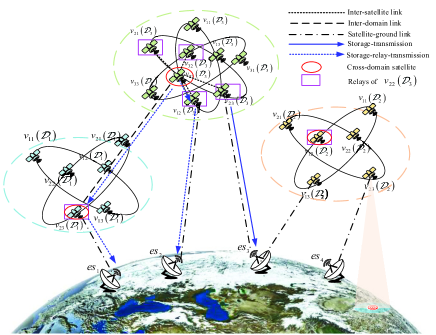
Figure 1: An illustration of the satellite network consisting of three domains.

In the satellite network, for any domain, the other domains can be selected as its auxiliary domains. When satellites complete their missions, they may also need to assist satellites of other domains to complete mission transmission. Two transmission modes can be chosen to offload missions to earth stations: 1) storage-transmission, i.e., satellites directly transmit missions to earth stations, and 2) storage-relay transmission, i.e., satellites transmit missions to the relay to offload. As shown in Fig. 1, the blue solid and dotted lines represent the two transmission modes, respectively. Furthermore, we make the following assumptions. Firstly, we divide the planning cycle into $T$ time slots and assume that the interval of time slot $t$ is fixed as $\tau$, where $t=\left\{1,2,\cdots,T\right\}$. Secondly, we consider the quasi-static network topology. Finally, we assume that only a transmission link can be established with at most one earth station for each satellite in each time slot.

We set that each satellite adopts the "one-satellite four-chain" mode to establish inter-satellite links (ISLs) in the intra-domain, which is widely used in typical satellite systems [28]. Furthermore, we set that satellites of different domains can transmit missions between domains by establishing inter-domain links (IDLs). Since not all satellites have IDLs in the actual network scenario, we select satellites at equal intervals in each domain to establish IDLs and name these satellites as cross-domain satellites (CSs). In addition, we set that each CS only establishes an IDL in each auxiliary domain. In summary, CSs can establish ISLs and IDLs, and the other satellites (i.e., non-cross-domain satellites (NCSs)) can only establish ISLs in the intra-domain. In light of the above rules, the intra-domain relays of each satellite are the satellites that establish the ISLs with itself and the inter-domain relays of CSs are the satellites that establish the IDLs with itself. As shown in Fig. 1, taking the satellite of $\mathcal{D}_{3}$ as an example, $v_{22}\left(\mathcal{D}_{3}\right)$ as the CS is marked with the red oval, and the intra- and inter-domain relays of $v_{22}\left(\mathcal{D}_{3}\right)$ are marked with the purple rectangle. $\mathfrak{\mathbb{\mathcal{R}}}\left(v_{ij}\left(\mathcal{D}_{k}\right),\mathcal{D}_{k^{\prime}}\right)$ is defined as the set of relays, where $k^{\prime}\in\left\{1,\cdots,K\right\}$ is the index of domains. If $k=k^{\prime}$, $\mathfrak{\mathbb{\mathcal{R}}}\left(v_{ij}\left(\mathcal{D}_{k}\right),\mathcal{D}_{k^{\prime}}\right)$ is represented as the set of intra-domain relays of $v_{ij}\left(\mathcal{D}_{k}\right)$. Otherwise, $\mathfrak{\mathbb{\mathcal{R}}}\left(v_{ij}\left(\mathcal{D}_{k}\right),\mathcal{D}_{k^{\prime}}\right)$ is the set of inter-domain relays of $v_{ij}\left(\mathcal{D}_{k}\right)$ in $D_{k^{\prime}}$.

III-B Channel Model

We elaborate on the channel model incorporating the ISL/IDL and satellite-ground link (SGL) in this subsection to characterize the impact of channel changes on the link transmission rate.

III-B1 ISL/IDL Channel Model

According to recent work [29, 30], the achievable transmission rate of the link from $v_{ij}\left(\mathcal{D}_{k}\right)$ to its relay in the $t$-th time slot, denoted by $Cs^{t}\left({\scriptstyle v_{ij}\left(\mathcal{D}_{k}\right),m}\right)$, can be expressed as:

$$Cs^{t}\left({\scriptstyle v_{ij}\left(\mathcal{D}_{k}\right),m}\right)=\frac{P_{sst}G_{tr}\left(v_{ij}\left(\mathcal{D}_{k}\right)\right)G_{re}\left(m\right)}{\mathcal{K}T_{n}\cdot\left(\nicefrac{{E_{b}}}{{N_{0}}}\right)_{req}\cdot\mathcal{L}^{t}\left(v_{ij}\left(\mathcal{D}_{k}\right),m\right)\cdot\mathcal{\textrm{M}}},$$ (1)

where $m\in\mathfrak{\mathbb{\mathcal{R}}}\left(v_{ij}\left(\mathcal{D}_{k}\right),\mathcal{D}_{k^{\prime}}\right)$ is the relay and $\mathcal{L}^{t}\left(v_{ij}\left(\mathcal{D}_{k}\right),m\right)$ is the free space loss shown as follows:

$$\mathcal{L}^{t}\left(v_{ij}\left(\mathcal{D}_{k}\right),m\right)=\left(\frac{4\pi\cdot Sl^{t}\left(v_{ij}\left(\mathcal{D}_{k}\right),m\right)\cdot\mathcal{F}}{c}\right)^{2}.$$ (2)

$Sl^{t}\left(v_{ij}\left(\mathcal{D}_{k}\right),m\right)$ is the slant range between $v_{ij}\left(\mathcal{D}_{k}\right)$ and its relay. $\mathcal{F}$ and $c$ are the communication center frequency and speed of light. $P_{sst}$ is the constant transmission power of satellites for ISL/IDL. $G_{tr}\left(v_{ij}\left(\mathcal{D}_{k}\right)\right)$ and $G_{re}\left(m\right)$ are the transmitting and receiving antenna gain respectively. Besides, $\mathcal{K}$ is the Boltzmann’s constant, and $T_{n}$ is the total system noise temperature. $\left(\nicefrac{{E_{b}}}{{N_{0}}}\right)_{req}$ and M are the required ratio of received energy-per-bit to noise-density, and link margin.

III-B2 SGL Channel Model

The achievable transmission rate of the link from $v_{ij}\left(\mathcal{D}_{k}\right)$ to $es_{g}$ in the $t$-th time slot is calculated using the Shannon formula [31], denoted by $Ce^{t}\left(v_{ij}\left(\mathcal{D}_{k}\right),es_{g}\right)$,

$$Ce^{t}\!\left(v_{ij}\left(\mathcal{D}_{k}\right)\!,\!es_{g}\right)\!=\!\mathcal{B}\!\cdot\!\textrm{log}_{2}\left(\!1\!+\!\mathcal{SNR}^{t}\!\left(\!v_{ij}\left(\mathcal{D}_{k}\right)\!,\!es_{g}\!\right)\right)\!,$$ (3)

where $\mathcal{SNR}^{t}\left(v_{ij}\left(\mathcal{D}_{k}\right),es_{g}\right)$ is the signal-to-noise ratio, expressed as:

$$\mathcal{SNR}^{t}\left(v_{ij}\left(\mathcal{D}_{k}\right),es_{g}\right)=\frac{P_{set}G_{tr}\left(v_{ij}\left(\mathcal{D}_{k}\right)\right)G_{re}\left(es_{g}\right)\mathcal{L}_{p}^{t}}{\mathcal{N}\cdot\mathcal{L}^{t}\left(v_{ij}\left(\mathcal{D}_{k}\right),es_{g}\right)}.$$ (4)

$P_{set}$ is the constant transmission power of satellites for SGL. $\mathcal{L}_{p}^{t}$ is the propagation loss. $\mathcal{N}$ is the noise. $\mathcal{B}$ is the available transmission bandwidth.

III-C Sparse Resource Representation

Due to the high-speed orbiting movement of satellites, the inter-satellite communication resources are highly dynamic [32]. We use the SRR scheme to characterize CR-IS of ISL/IDL, denoted by $l^{t}\left(v_{ij}\left(\mathcal{D}_{k}\right),m\right)$, where $m\in\mathfrak{\mathbb{\mathcal{R}}}\left(v_{ij}\left(\mathcal{D}_{k}\right)\right)$ is the relay and $\mathfrak{\mathbb{\mathcal{R}}}\left(v_{ij}\left(\mathcal{D}_{k}\right)\right)$ $=\left\{\mathfrak{\mathbb{\mathcal{R}}}\left(v_{ij}\left(\mathcal{D}_{k}\right),\mathcal{D}_{k^{\prime}}\right)\left|k^{\prime}\!\in\!\left\{1,2,\cdots,K\right\}\right.\right\}$ is the set of all relays of $v_{ij}\left(\mathcal{D}_{k}\right)$ [27].

The SRR scheme characterizes the CR-IS of ISL/IDL in real-time by constructing the satellite orbit feature matrix (SOFM) of each domain to deduce the network topology. Specifically, the SOFM of each domain consists of orbit parameters representing the satellite position of the initial time slot, including the orbit height $h_{i}$, eccentricity $e_{i}$, inclination $I_{i}$, argument of perigee $\Omega_{i}$, right ascension of ascending node $RA_{i}$, and mean anomaly in the first time slot $\overline{TA_{ij}^{1}}$, where $i\in\left\{1,2,\cdots,\mathcal{I}_{k}\right\},j\in\left\{1,2,\cdots,\mathcal{J}_{k}\right\}$. Using the position information of the satellites obtained by searching the SOFM, the maximum geocentric angle $\theta^{max}\left(v_{ij}\left(\mathcal{D}_{k}\right)\text{,$v_{ij}\left(\mathcal{D}_{k\text{'}}\right)$}\right)$ and geocentric angle $\theta^{t}\left(v_{ij}\left(\mathcal{D}_{k}\right)\text{,$v_{ij}\left(\mathcal{D}_{k\text{'}}\right)$}\right)$ in the $t$-th time slot can be calculated to acquire the CR-IS of ISL/IDL. If $\theta^{t}\left(v_{ij}\left(\mathcal{D}_{k}\right)\text{,$v_{ij}\left(\mathcal{D}_{k\text{'}}\right)$}\right)\leq\theta^{max}\left(v_{ij}\left(\mathcal{D}_{k}\right)\text{,$v_{ij}\left(\mathcal{D}_{k\text{'}}\right)$}\right)$, the ISL/IDL can be established, i.e., $l^{t}\left(v_{ij}\left(\mathcal{D}_{k}\right),m\right)=1$. Otherwise, $l^{t}\left(v_{ij}\left(\mathcal{D}_{k}\right),m\right)=0$.

III-D Mission Priority Model

We define that the mission of each domain consists of a 5-tuple. Specifically, $\mathcal{M}^{t}\left(v_{ij}\left(\mathcal{D}_{k}\right)\right)$=$\left\{\mathcal{P}\left(\mathcal{M}_{k}\right),\rho\left(\mathcal{M}_{k}\right),t,\mathcal{R}s\left(\mathcal{M}_{k}\right),v_{ij}\left(\mathcal{D}_{k}\right)\right\}$ represents the mission collected/generated by $v_{ij}\left(\mathcal{D}_{k}\right)$ in the $t$-th time slot, where $\mathcal{M}_{k}$ represents the mission of $\mathcal{D}_{k}$. $\mathcal{P}\left(\mathcal{M}_{k}\right)$ represents the priority of $\mathcal{M}_{k}$, which is used to determine the order in which each mission is served in different domains. $\rho\left(\mathcal{M}_{k}\right)$ represents the data volume of $\mathcal{M}_{k}$. $t$ represents the mission collected/generated in the $t$-th time slot. $\mathcal{R}s\left(\mathcal{M}_{k}\right)$ represents the survival time slots of $\mathcal{M}_{k}$. Furthermore, $\mathcal{R}s\left(\mathcal{M}_{k}\right)$ is decremented with a step size of 1 during the CMS, i.e., the remaining survival time slot of each mission is different in each time slot, and when decremented to 0, the mission will be deleted from the on-board memory, i.e., the mission is not completed. $v_{ij}\left(\mathcal{D}_{k}\right)$ is used to clarify the reward allocation during training. In this paper, we set that there are common missions and burst missions in each domain and do not consider the splitting of missions, i.e., each mission must complete the transmission on one path.

We extract mission attributes from three aspects (i.e., the data volume of the mission, mission arrival rate, and delay tolerance) and model them as the mission priority to effectively characterize the differentiation of mission demands. The calculation formulation of mission priority is as follows [33]:

$$\mathcal{P}\left(\mathcal{M}_{k}\right)=\stackrel{{\scriptstyle[}}{{\scriptstyle f=1}}]{{\scriptstyle\mathcal{F}}}{\sum}\mathcal{W}_{f}\left(\mathcal{M}_{k}\right)\cdot\mathcal{V}_{f}\left(\mathcal{M}_{k}\right),$$ (5)

where $\mathcal{F}=3$ is the number of the mission attributes. $\mathcal{W}_{f}\left(\mathcal{M}_{k}\right)$ represents the weight of the $f$-th mission attribute of $\mathcal{M}_{k}$, which examines the degree of influence of each mission attribute on the priority of the mission. $\mathcal{W}_{f}\left(\mathcal{M}_{k}\right)$ is shown as follows:

$$\mathcal{W}_{f}\left(\mathcal{M}_{k}\right)=\frac{\stackrel{{\scriptstyle[}}{{y}}=1]{\mathcal{F}}{\sum}\mathcal{\textrm{I}}_{fy}\left(\mathcal{M}_{k}\right)}{\stackrel{{\scriptstyle[}}{{x}}=1]{\mathcal{F}}{\sum}\stackrel{{\scriptstyle[}}{{y}}=1]{\mathcal{F}}{\sum}\mathcal{\textrm{I}}_{xy}\left(\mathcal{M}_{k}\right)},\>\left\{f=1,\cdots,\mathcal{F}\right\},$$ (6)

where $\mathcal{\textrm{I}}_{xy}\left(\mathcal{M}_{k}\right)$ is a score obtained by comparing the importance of each mission attribute using a 0-1 scoring method to effectively evaluate the weight of each mission attribute in $\mathcal{M}_{k}$. $\mathcal{\textrm{I}}_{xy}\left(\mathcal{M}_{k}\right)$ is expressed as follows:

$$\mathcal{\textrm{I}}_{xy}\left(\mathcal{M}_{k}\right)=\begin{cases}1&x>y,\\ 0.5&x=y,\\ 0&x<y.\end{cases}$$ (7)

$\mathcal{V}_{f}\left(\mathcal{M}_{k}\right)$ represents the quantitative value of the $f$-th mission attribute of $\mathcal{M}_{k}$, and the specific value reflects the relationship of the $f$-th mission attribute among different domain missions. For example, the NM should be offloaded in a timely to guarantee its effectiveness, and the OM has a higher delay tolerance than the NM. Therefore, the quantitative value of the delay tolerance attribute of the NM is set higher than that of OM.

III-E Energy Model

In this subsection, we introduce the energy consumption model and the energy harvesting model, respectively. To model the energy consumption of satellites, we define $\mathcal{H}_{\mathcal{M}_{k^{\prime}}}^{t}\left(v_{ij}\left(\mathcal{D}_{k}\right),m\right)$ as the number of $\mathcal{M}_{k^{\prime}}$ that $v_{ij}\left(\mathcal{D}_{k}\right)$ transmits to its relay and $\mathcal{H}_{\mathcal{M}_{k^{\prime}}}^{t}\left(v_{ij}\left(\mathcal{D}_{k}\right),es_{g}\right)$ as the number of $\mathcal{M}_{k^{\prime}}$ that $v_{ij}\left(\mathcal{D}_{k}\right)$ transmits to $es_{g}$ during the $t$-th time slot. Hereafter, we elaborate on the two models.

The energy consumption of $v_{ij}\left(\mathcal{D}_{k}\right)$ for transmitting data during the $t$-th time slot, is expressed as:

$$\begin{array}[]{cc}E_{tr}^{t}\left(v_{ij}\left(\mathcal{D}_{k}\right)\right)\!\!=&\!\!\!\!\underset{{\scriptstyle m\in\mathfrak{\mathbb{\mathcal{R}}}\left(v_{ij}\left(\mathcal{D}_{k}\right)\right)}}{\sum}\!\!\frac{\mathcal{X}^{t}\left(v_{ij}\left(\mathcal{D}_{k}\right),m\right)}{Cs^{t}\left(v_{ij}\left(\mathcal{D}_{k}\right),m\right)}\!\cdot\!P_{sst}\\ &+\stackrel{{\scriptstyle[}}{{\scriptstyle g=1}}]{{\scriptstyle N}}{\sum}\frac{{\scriptstyle\mathcal{X}^{t}\left(v_{ij}\left(\mathcal{D}_{k}\right),es_{g}\right)}}{{\scriptstyle Ce^{t}\left(v_{ij}\left(\mathcal{D}_{k}\right),es_{g}\right)}}\cdot P_{set},\end{array}$$ (8)

where $\mathcal{X}^{t}\left(v_{ij}\left(\mathcal{D}_{k}\right),m\right)=\stackrel{{\scriptstyle[}}{{k}}^{\prime}=1]{K}{\sum}\mathcal{H}_{\mathcal{M}_{k^{\prime}}}^{t}\left(v_{ij}\left(\mathcal{D}_{k}\right),m\right)\cdot\rho\left(\mathcal{M}_{k^{\prime}}\right)$ represents the data volume that $v_{ij}\left(\mathcal{D}_{k}\right)$ transmits to its relay, and $\mathcal{X}^{t}\left(v_{ij}\left(\mathcal{D}_{k}\right),es_{g}\right)=\stackrel{{\scriptstyle[}}{{k}}^{\prime}=1]{K}{\sum}\mathcal{H}_{\mathcal{M}_{k^{\prime}}}^{t}\left(v_{ij}\left(\mathcal{D}_{k}\right),es_{g}\right)\cdot\rho\left(\mathcal{M}_{k^{\prime}}\right)$ represents the data volume that $v_{ij}\left(\mathcal{D}_{k}\right)$ transmits to $es_{g}$.

The energy consumption of $v_{ij}\left(\mathcal{D}_{k}\right)$ for receiving data is denoted as $E_{r}^{t}\left(v_{ij}\left(\mathcal{D}_{k}\right)\right)$ during the $t$-th time slot, as follows:

$$E_{r}^{t}\left(v_{ij}\left(\mathcal{D}_{k}\right)\right)\!\!=\underset{{\scriptstyle m\in\mathbb{R}\left(v_{ij}\left(\mathcal{D}_{k}\right)\right)}}{\sum}\!\!\frac{\widehat{\mathcal{X}^{t}}\left(m,v_{ij}\left(\mathcal{D}_{k}\right)\right)}{Cs^{t}\left(m,v_{ij}\left(\mathcal{D}_{k}\right)\right)}\!\cdot\!P_{sr},$$ (9)

where $\mathbb{R}\left(v_{ij}\left(\mathcal{D}_{k}\right)\right)\!=\!\left\{\!v_{i^{\prime}j^{\prime}}\!\left(\mathcal{D}_{k^{\prime}}\right)\!\!\right.\left|\!v_{ij}\left(\mathcal{D}_{k}\right)\!\in\!\mathfrak{\mathcal{R}\!}\left(\!v_{i^{\prime}j^{\prime}}\left(\mathcal{D}_{k^{\prime}}\right)\!,\!\mathcal{D}_{k}\right)\!,\right.$ $\left.\left.i^{\prime}\in\left\{1,2,\cdots,\mathcal{I}_{k^{\prime}}\right\}\!,j^{\prime}\in\left\{1,2,\right.\cdots,\mathcal{J}_{k^{\prime}}\right\},k^{\prime}\!\in\!\left\{1,2,\cdots,K\right\}\right\}$ is the set of satellites that can transmit missions to $v_{ij}\left(\mathcal{D}_{k}\right)$. $\widehat{\mathcal{X}^{t}}\left(m,v_{ij}\left(\mathcal{D}_{k}\right)\right)$ represents the data volume received by $v_{ij}\left(\mathcal{D}_{k}\right)$ originating from $m$. It should be noted that due to the limitation of storage capacity and remaining battery energy, $\widehat{\mathcal{X}^{t}}\left(m,v_{ij}\left(\mathcal{D}_{k}\right)\right)\leq\mathcal{X}^{t}\left(m,v_{ij}\left(\mathcal{D}_{k}\right)\right)$. $P_{sr}$ is the reception power of satellites.

Moreover, we define the energy consumption of $v_{ij}\left(\mathcal{D}_{k}\right)$ for nominal operation during the $t$-th time slot, denoted by $E_{o}^{t}\left(v_{ij}\left(\mathcal{D}_{k}\right)\right)$, is expressed as follows:

$$E_{o}^{t}\left(v_{ij}\left(\mathcal{D}_{k}\right)\right)=P_{o}\cdot\tau,$$ (10)

where $P_{o}$ is the nominal operation power.

The total energy consumption of $v_{ij}\left(\mathcal{D}_{k}\right)$ during the $t$-th time slot consists of the above energy consumption items, denoted by $E_{c}^{t}\left(v_{ij}\left(\mathcal{D}_{k}\right)\right)$, as follows:

$$E_{c}^{t}\!\left(v_{ij}\left(\mathcal{D}_{k}\right)\right)\!\!=\!\!E_{tr}^{t}\!\left(\!v_{ij}\left(\mathcal{D}_{k}\right)\!\right)\!+\!E_{r}^{t}\!\left(\!v_{ij}\left(\mathcal{D}_{k}\right)\!\right)\!+\!E_{o}^{t}\!\left(\!v_{ij}\left(\mathcal{D}_{k}\right)\!\right)\!.$$ (11)

We denote $E_{h}^{t}\left(v_{ij}\left(\mathcal{D}_{k}\right)\right)$ as the harvested energy of $v_{ij}\left(\mathcal{D}_{k}\right)$ during the $t$-th time slot and determine it in advance according to orbital dynamics. $E_{h}^{t}\left(v_{ij}\left(\mathcal{D}_{k}\right)\right)$ is expressed as:

$$E_{h}^{t}\left(v_{ij}\left(\mathcal{D}_{k}\right)\right)=P_{h}\cdot\min\left\{\tau,y^{t}\left(v_{ij}\left(\mathcal{D}_{k}\right)\right)\right\},$$ (12)

where $P_{h}$ is the energy collection rate. $y^{t}\left(v_{ij}\left(\mathcal{D}_{k}\right)\right)$ is the duration that the satellite is covered by the sun at the beginning of the $t$-th time slot. When the satellite is completely eclipsed by the Earth in the $t$-th time slot, $y^{t}\left(v_{ij}\left(\mathcal{D}_{k}\right)\right)=0$.

IV Formulation

In this section, we study the CMS problem of maximizing the number of completed missions satisfying the resources and link constraints. First of all, we present the related constraints, and then the proposed CMS problem is formulated based on these constraints. Finally, we convert it into the MDP-based HCMS problem to solve.

IV-A Related Constraints Modeling

IV-A1 Storage Resource Constraint

The total data volume of all missions stored on each satellite cannot exceed its storage capacity,

$$\mathcal{B}^{t}\left(v_{ij}\left(\mathcal{D}_{k}\right)\right)\!+\widehat{\mathcal{X}^{t}}\left(v_{ij}\left(\mathcal{D}_{k}\right)\right)\!-\mathcal{X}^{t}\left(v_{ij}\left(\mathcal{D}_{k}\right)\right)\!+\!\rho\left(\mathcal{M}_{k}\right)\!\leq\!\mathcal{B}_{max}.$$ (13)

where $\mathcal{B}^{t}\left(v_{ij}\left(\mathcal{D}_{k}\right)\right)$ is the total data volume of missions stored in $v_{ij}\left(\mathcal{D}_{k}\right)$ at the beginning of $t$-th time slot, $\widehat{\mathcal{X}^{t}}\left(v_{ij}\left(\mathcal{D}_{k}\right)\right)=\underset{{\scriptstyle m\in\mathbb{R}\left(v_{ij}\left(\mathcal{D}_{k}\right)\right)}}{\sum}\!\!\widehat{\mathcal{X}^{t}}\left(m,v_{ij}\left(\mathcal{D}_{k}\right)\right)$ is the total data volume received by $v_{ij}\left(D_{k}\right)$, $\mathcal{X}^{t}\left(v_{ij}\left(\mathcal{D}_{k}\right)\right)=\!\!\underset{{\scriptstyle{\scriptstyle m\in\mathfrak{\mathbb{\mathcal{R}}}\left(v_{ij}\left(\mathcal{D}_{k}\right)\right)}}}{\sum}\!\!\mathcal{X}^{t}\left(v_{ij}\left(\mathcal{D}_{k}\right),m\right)+\!\!\!\stackrel{{\scriptstyle[}}{{\scriptstyle g=1}}]{{\scriptstyle N}}{\sum}\!\!\mathcal{X}^{t}\left(v_{ij}\left(\mathcal{D}_{k}\right),es_{g}\right)$ is the total data volume that can be transmitted by $v_{ij}\left(\mathcal{D}_{k}\right)$, and $\mathcal{B}_{max}$ is the storage capacity.

IV-A2 Energy Resource Constraint

The battery capacity of each satellite is also limited, and the normal operation of the satellite in shadow should be maintained. Therefore, all energy cannot be fully used for the mission transmission and reception, i.e.,

$$E^{t}\left(v_{ij}\left(\mathcal{D}_{k}\right)\right)-E_{c}^{t}\left(v_{ij}\left(\mathcal{D}_{k}\right)\right)\geq E_{min},$$ (14)

and the battery energy cannot exceed the battery capacity, i.e.,

$$E^{t}\left(v_{ij}\left(\mathcal{D}_{k}\right)\right)+\widetilde{E_{h}^{t}}\left(v_{ij}\left(\mathcal{D}_{k}\right)\right)-E_{c}^{t}\left(v_{ij}\left(\mathcal{D}_{k}\right)\right)\leq E_{max},$$ (15)

where $E^{t}\left(v_{ij}\left(\mathcal{D}_{k}\right)\right)$ is the residual energy in $v_{ij}\left(\mathcal{D}_{k}\right)$ at the beginning of the $t$-th time slot, $E_{min}=E_{max}-\eta\cdot E_{max}$ represents the minimum residual energy of the battery and $\eta$ represents the maximum discharge depth of the battery. $\widetilde{E_{h}^{t}}\left(v_{ij}\left(\mathcal{D}_{k}\right)\right)\leq E_{h}^{t}\left(v_{ij}\left(\mathcal{D}_{k}\right)\right)$ is the actual harvested energy, and $E_{max}$ is the battery capacity.

IV-A3 Communication Resource Constraints

During the mission transmission, since the transmission rate of the link is limited, each satellite transmits the total data volume that cannot exceed the link capacity. Furthermore, we consider that each satellite only transmits missions to one relay or one earth station in each time slot. Therefore, binary variables $u^{t}\left(v_{ij}\left(\mathcal{D}_{k}\right),m\right)$ and $u^{t}\left(v_{ij}\left(\mathcal{D}_{k}\right),es_{g}\right)$ $\in\left\{0,1\right\}$ are introduced to represent whether the links from $v_{ij}\left(\mathcal{D}_{k}\right)$ to the relays/earth stations are used, 1 if used and 0 otherwise. The communication resource constraints are as follows:

$$\begin{array}[]{cc}\mathcal{X}^{t}\!\left(\!v_{ij}\left(\mathcal{D}_{k}\right)\!\right)\!\leq&\!\!\!\!\!\left(\!\!\underset{{\scriptstyle{\scriptstyle m\in\mathfrak{\mathbb{\mathcal{R}}}\left(v_{ij}\left(\mathcal{D}_{k}\right)\right)}}}{\sum}\!\!\!\!\!\!\!Cs^{t}\left(v_{ij}\left(\mathcal{D}_{k}\right),m\right)\!\cdot\!u^{t}\left(v_{ij}\!\left(\mathcal{D}_{k}\right)\!,\!m\!\right)\right.\\ &\left.\!\!\!\!\!\!\!\!\!\!\!\!\!\!\!+\!\!\stackrel{{\scriptstyle[}}{{\scriptstyle g=1}}]{{\scriptstyle N}}{\sum}Ce^{t}\left(v_{ij}\left(\mathcal{D}_{k}\right),es_{g}\right)\!\cdot\!u^{t}\left(\!v_{ij}\left(\mathcal{D}_{k}\right)\!,\!es_{g}\right)\!\right)\!\cdot\!\tau\end{array}$$ (16)

IV-A4 Link Constraint

Since we consider that each satellite only transmits missions to one relay or one earth station in each time slot, only one link can be selected for the mission transmission of each satellite in each time slot,

$$\underset{{\scriptstyle m\in\mathfrak{\mathbb{\mathcal{R}}}\left(v_{ij}\left(\mathcal{D}_{k}\right)\right)}}{\sum}\!\!\!\!\!\!\!\!\!u^{t}\left(v_{ij}\left(\mathcal{D}_{k}\right),m\right)\!\!+\!\!\stackrel{{\scriptstyle[}}{{\scriptstyle g=1}}]{{\scriptstyle N}}{\sum}\!u^{t}\!\left(\!v_{ij}\left(\mathcal{D}_{k}\right)\!,\!es_{g}\right)\!\!=\!\!1,$$ (17)

IV-B Problem Formulation

To achieve effective offloading of missions in each domain, we jointly consider the resources and link constraints to maximize the number of completed missions in the whole network. Mathematically, this problem can be formulated as follows:

$$\begin{array}[]{c}\!\!\negthickspace\negthickspace\textrm{CMS:\!\!}\underset{\underset{{\scriptstyle u^{t}\left(\!v_{ij}\left(\mathcal{D}_{k}\right),es_{g}\!\right)}}{u^{t}\left(\!v_{ij}\left(\mathcal{D}_{k}\right),m\!\right)}}{\max}\underset{k\in\left\{1,2,\cdots,K\right\}}{\sum}\mathbb{C}\left(\mathcal{D}_{k}\right)\\ \textrm{s.t.}\enskip\left(\ref{eq:Storage}\right)-\left(\ref{eq:Link}\right),\end{array}$$ (18)

where $\mathcal{\mathbb{C}}\left(\mathcal{D}_{k}\right)=\stackrel{{\scriptstyle[}}{{\scriptstyle i=1}}]{{\scriptscriptstyle\mathcal{{\scriptstyle I}}_{k}}}{\sum}\stackrel{{\scriptstyle[}}{{\scriptstyle j=1}}]{{\scriptscriptstyle\mathcal{{\scriptstyle J}}_{k}}}{\sum}\stackrel{{\scriptstyle[}}{{\scriptstyle t=1}}]{{\scriptstyle T}}{\sum}\stackrel{{\scriptstyle[}}{{\scriptstyle g=1}}]{{\scriptstyle N}}{\sum}\mathcal{H}^{t}\left(v_{ij}\left(\mathcal{D}_{k}\right),es_{g}\right)$ is the total number of completed missions in $\mathcal{D}_{k}$, and $\mathcal{H}^{t}\left(v_{ij}\left(\mathcal{D}_{k}\right),es_{g}\right)=\stackrel{{\scriptstyle[}}{{k}}^{\prime}=1]{K}{\sum}\mathcal{H}_{\mathcal{M}_{k^{\prime}}}^{t}\left(v_{ij}\left(\mathcal{D}_{k}\right),es_{g}\right).$ It should be noted that although this formulation only includes missions that are offloaded on the SGL, the missions may be offloaded by mode (2), i.e., storage-relay-transmission.

In this formulation, decision variables are integer variables. Therefore, the CMS problem is the integer linear programming problem, which is NP-hard and mission scheduling demands are dynamic, which strengthens the solution complexity of the problem. Furthermore, with the continuous increase of satellite systems and the continuous expansion of the constellations’ scale, the number of decision variables for the CMS problem increases rapidly, which makes it more difficult to solve the CMS problem using the traditional optimization method. Therefore, we need to convert the CMS problem so that it can be solved efficiently.

IV-C CMS Problem Conversion

In this subsection, exploiting the Markov property of the CMS process and the correlation of intra- and inter-domain mission scheduling, we convert the CMS problem into the MDP-based HCMS problem (including TMS and BMS problems) by constructing the TMS and BMS models of reward association. Specifically, the BMS problem is formulated to solve the mission scheduling in the domain to achieve intra-domain resource collaboration, and the TMS problem is formulated to solve the mission scheduling in the inter-domain to achieve inter-domain resource collaboration.

IV-C1 BMS Problem

Before describing the BMS problem, we first define the state information of each satellite. Due to the obvious differences in the resources of CSs and NCSs and each domain mission attribute, we adopt the relative value of the resource states and the mission states to replace the true value to describe each satellite. Specifically, we set that the state of each satellite $s^{t}\left(v_{ij}\left(\mathcal{D}_{k}\right)\right)$ consists of a 4-tuple, i.e.,

$$\begin{array}[]{cc}s^{t}\left(v_{ij}\left(\mathcal{D}_{k}\right)\right)=&\!\!\!\!\!\!\left(\widetilde{\mathcal{B}^{t}}\left(v_{ij}\left(\mathcal{D}_{k}\right)\right),\widetilde{E^{t}}\left(v_{ij}\left(\mathcal{D}_{k}\right)\right)\text{,}\right.\\ &\left.\widetilde{Ce^{t}}\left(v_{ij}\left(\mathcal{D}_{k}\right)\right),\widetilde{\mathcal{R}s^{t}}\left(v_{ij}\left(\mathcal{D}_{k}\right)\right)\right),\end{array}$$ (19)

where $\widetilde{\mathcal{B}^{t}}\left(v_{ij}\left(\mathcal{D}_{k}\right)\right)$ is the relative value that characterizes storage occupied, $\widetilde{E^{t}}\left(v_{ij}\left(\mathcal{D}_{k}\right)\right)$ is the relative value that characterizes remaining available battery energy, $\widetilde{Ce^{t}}\left(v_{ij}\left(\mathcal{D}_{k}\right)\right)$ indicates whether can directly offload the missions to earth stations, and $\widetilde{\mathcal{R}s^{t}}\left(v_{ij}\left(\mathcal{D}_{k}\right)\right)$ is the average of the remaining survival time slots for all missions stored on $v_{ij}\left(\mathcal{D}_{k}\right)$ at the beginning of the $t$-th time slot.

Specifically, $\widetilde{\mathcal{B}^{t}}\left(v_{ij}\left(\mathcal{D}_{k}\right)\right)=\nicefrac{{\mathcal{B}_{max}}}{{\mathcal{B}^{t}\left(v_{ij}\left(\mathcal{D}_{k}\right)\right)}}$ and if $\mathcal{B}^{t}\left(v_{ij}\left(\mathcal{D}_{k}\right)\right)=0$, $\widetilde{\mathcal{B}^{t}}\left(v_{ij}\left(\mathcal{D}_{k}\right)\right)=\mathcal{B}_{max}$. $\mathcal{B}^{t}\left(v_{ij}\left(\mathcal{D}_{k}\right)\right)\in\left[0,\mathcal{B}_{max}\right]$ is denoted as

$$\!\begin{array}[]{cc}\mathcal{B}^{t}\left(v_{ij}\left(\mathcal{D}_{k}\right)\right)\!=&\mathcal{B}^{t-1}\left(v_{ij}\left(\mathcal{D}_{k}\right)\right)\!+\!\widehat{\mathcal{X}^{t-1}}\left(v_{ij}\left(\mathcal{D}_{k}\right)\right)\!\\ &-\!\mathcal{X}^{t-1}\left(v_{ij}\left(\mathcal{D}_{k}\right)\right)\!+\!\rho\left(\mathcal{M}_{k}\right)\!.\end{array}$$ (20)

$\widetilde{E^{t}}\left(\!v_{ij}\left(\mathcal{D}_{k}\right)\!\right)\!=\!\nicefrac{{E^{t}\left(v_{ij}\left(\mathcal{D}_{k}\right)\right)}}{{\left(E_{min}+E_{o}^{t}\left(v_{ij}\left(\mathcal{D}_{k}\right)\right)\right)}}$. $E^{t}\left(\!v_{ij}\left(\mathcal{D}_{k}\right)\!\right)$ $\in\left[0,E_{max}\right]$ is denoted as

$$E^{t}\!\!\left({\scriptstyle v_{ij}\left(\mathcal{D}_{k}\right)}\right)\!=\!E^{t-1}\!\left({\scriptstyle v_{ij}\left(\mathcal{D}_{k}\right)}\right)\!+\!\widetilde{E_{h}^{t-1}\!}\left({\scriptstyle v_{ij}\left(\mathcal{D}_{k}\right)}\right)\!-\!E_{c}^{t-1}\!\left({\scriptstyle v_{ij}\left(\mathcal{D}_{k}\right)}\right)\!.$$ (21)

$\widetilde{Ce^{t}}\left(v_{ij}\left(\mathcal{D}_{k}\right)\right)$ is the average rate of available SGLs by $v_{ij}\left(\mathcal{D}_{k}\right)$. If there is no available SGL, $\widetilde{Ce^{t}}\left(v_{ij}\left(\mathcal{D}_{k}\right)\right)$=0.

Since the satellites affect the state information of each other when transmitting missions, to achieve efficient mission scheduling of the whole network, we focus on a multi-agent network scenario and adopt the joint state information (JSI) of multiple satellites to make a decision. Specifically, in the BMS problem, we set each satellite to exchange its local state information with its intra-domain relays, and processes them. Further, each satellite constructs the JSI of the intra-domain using processed state information of its own and intra-domain relays, expressed as

$$\textrm{S}_{BMS}^{t}\left(v_{ij}\left(\mathcal{D}_{k}\right)\right)\!=\!\left[\widehat{s^{t}}\left({\scriptstyle v_{ij}\left(\mathcal{D}_{k}\right)}\right)\right]\cup\left[\widehat{s^{t}}\left({\scriptstyle m}\right)\right]_{m\in\mathfrak{\mathbb{\mathcal{R}}}\left(v_{ij}\left(\mathcal{D}_{k}\right),\mathcal{D}_{k}\right)}\!,$$ (22)

where $\widehat{s^{t}}\left({\scriptstyle v_{ij}\left(\mathcal{D}_{k}\right)}\right)\!=\!\left(\!\widetilde{\mathcal{B}^{t}}\left({\scriptstyle v_{ij}\left(\mathcal{D}_{k}\right)}\right),\!\widetilde{E^{t}}\left({\scriptstyle v_{ij}\left(\mathcal{D}_{k}\right)}\right),\!\widetilde{Ce^{t}}\left({\scriptstyle v_{ij}\left(\mathcal{D}_{k}\right)}\right)\!,\right.$ $\left.\widehat{\mathcal{R}s^{t}}\left({\scriptstyle v_{ij}\left(\mathcal{D}_{k}\right)}\right)\right)$ and $\widehat{s^{t}}\left({\scriptstyle m}\right)\!=\!\left(\!\widetilde{\mathcal{B}^{t}\!}\left({\scriptstyle m}\right)\!,\!\widetilde{E^{t}\!}\left({\scriptstyle m}\right)\!,\!\widetilde{Ce^{t}\!}\left({\scriptstyle m}\right)\!,\!\widehat{\mathcal{R}s^{t}\!}\left({\scriptstyle m}\right)\!\right)$ are the processed state information. $\widehat{\mathcal{R}s^{t}}\left({\scriptstyle v_{ij}\left(\mathcal{D}_{k}\right)}\right)=\nicefrac{{\widetilde{\mathcal{R}s^{t}}\left(v_{ij}\left(\mathcal{D}_{k}\right)\right)}}{{\widetilde{\mathcal{R}s^{t}}\left(v_{ij}\left(\mathcal{D}_{k}\right)\right)}}$ represents the relative value of the average of the remaining survival time slots, and if $\widetilde{\mathcal{R}s^{t}}\left(v_{ij}\left(\mathcal{D}_{k}\right)\right)=0$, $\widehat{\mathcal{R}s^{t}}\left({\scriptstyle v_{ij}\left(\mathcal{D}_{k}\right)}\right)=0$. Similarly, $\widehat{\mathcal{R}s^{t}}\left(m\right)=\nicefrac{{\widetilde{\mathcal{R}s^{t}}\left(v_{ij}\left(\mathcal{D}_{k}\right)\right)}}{{\widetilde{\mathcal{R}s^{t}}\left(m\right)}}$, and if $\widetilde{\mathcal{R}s^{t}}\left(m\right)=0$, $\widehat{\mathcal{R}s^{t}}\left(m\right)=\widetilde{\mathcal{R}s^{t}}\left(v_{ij}\left(\mathcal{D}_{k}\right)\right)$.

$$\textrm{Pr}_{BMS}^{t}\left(v_{ij}\left(\mathcal{D}_{k}\right)\right)=\begin{cases}\stackrel{{\scriptstyle[}}{{\scriptstyle g=1}}]{{\scriptstyle N}}{\sum}\mathcal{X}^{t}\left({\scriptstyle a_{BMS}^{t}\left(v_{ij}\left(\mathcal{D}_{k}\right)\right),es_{g}}\right),&if\>a_{BMS}^{t}\left(v_{ij}\left(\mathcal{D}_{k}\right)\right)=v_{ij}\left(\mathcal{D}_{k}\right),\\ \stackrel{{\scriptstyle[}}{{\scriptstyle g=1}}]{{\scriptstyle N}}{\sum}\widetilde{\mathcal{X}^{t}}\left({\scriptstyle a_{BMS}^{t}\left(v_{ij}\left(\mathcal{D}_{k}\right)\right),es_{g}}\right),&if\>a_{BMS}^{t}\left(v_{ij}\left(\mathcal{D}_{k}\right)\right)\neq v_{ij}\left(\mathcal{D}_{k}\right)\cap\widetilde{Ce^{t}}\left(v_{ij}\left(\mathcal{D}_{k}\right)\right)=0\\ &\cap\,missions\,originate\,from\,v_{ij}\left(\mathcal{D}_{k}\right),\\ 0,&else,\end{cases}$$ (23)

 

The feasible action set of the BMS problem $\mathcal{\textrm{A}}_{BMS}^{t}\left(v_{ij}\left(\mathcal{D}_{k}\right)\right)$ corresponds to the index of optional intra-domain relays and the earth station, which characterizes the satellites that can be selected to perform mission transmission during mission scheduling, expressed as $\mathcal{\textrm{A}}_{BMS}^{t}\left(v_{ij}\left(\mathcal{D}_{k}\right)\right)\!\!=\!\!\left\{a_{BMS}^{t}\left(v_{ij}\left(\mathcal{D}_{k}\right)\right)\!\!=\!\!p\left|l^{t}\left(v_{ij}\left(\mathcal{D}_{k}\right),p\right)\!=\!1,\!p\!\in\!\left\{\!\mathfrak{\mathbb{\mathcal{R}}\!}\left(v_{ij}\left(\mathcal{D}_{k}\right)\!,\!\mathcal{D}_{k}\right)\right.\right.\right.$ $\left.\left.\cup v_{ij}\left(\mathcal{D}_{k}\right)\right\}\right\},$ where $v_{ij}\left(\mathcal{D}_{k}\right)$ is used to indicate that the missions are transmitted to the earth station, if $\exists l^{t}\left(v_{ij}\left(\mathcal{D}_{k}\right),es_{g}\right)\!=\!1$, $l^{t}\left(v_{ij}\left(\mathcal{D}_{k}\right),v_{ij}\left(\mathcal{D}_{k}\right)\right)\!=\!1$, otherwice, $l^{t}\left(v_{ij}\left(\mathcal{D}_{k}\right),v_{ij}\left(\mathcal{D}_{k}\right)\right)=0$. $l^{t}\left(v_{ij}\left(\mathcal{D}_{k}\right),es_{g}\right)$ is the connection relationship of SGL.

For the reward of the BMS problem, we set it consists of two parts, namely, 1) the profit value $\textrm{Pr}_{BMS}^{t}\left(v_{ij}\left(\mathcal{D}_{k}\right)\right)$: the data volume of missions successfully transmitted to the earth station, denoted as (23), where $\widetilde{\mathcal{X}^{t}}\left({\scriptstyle a_{BMS}^{t}\left(v_{ij}\left(\mathcal{D}_{k}\right)\right),es_{g}}\right)$ is the data volume of missions from $v_{ij}\left(\mathcal{D}_{k}\right)$ successfully transmitted to the earth station via the transmission mode 2); 2) the penalty value $\textrm{Pe}_{BMS}^{t}\left(v_{ij}\left(\mathcal{D}_{k}\right)\right)$: the data volume of missions failed to be received by the relay when using the transmission mode 2), denoted as

$$\begin{array}[]{cc}\!\!\textrm{Pe}_{BMS}^{t}\left({\scriptstyle{\textstyle v_{ij}\left(\mathcal{D}_{k}\right)}}\right)\!=&\!\!\!\!\!\!\!\!\!\!\mathcal{X}^{t}\left({\scriptstyle{\textstyle v_{ij}\left(\mathcal{D}_{k}\right),a_{BMS}^{t}\left(\!v_{ij}\left(\mathcal{D}_{k}\right)\!\right)}}\right)\\ &\!\!\!\!\!\!\!\!\!\!-\widehat{\mathcal{X}^{t}}\left({\textstyle v_{ij}\left(\mathcal{D}_{k}\right),a_{BMS}^{t}\left(\!v_{ij}\left(\mathcal{D}_{k}\right)\!\right)}\right),\end{array}$$ (24)

then we define that (23) minus (24) as the reward, i.e.,

$$\textrm{R}_{BMS}^{t}\left({\scriptstyle{\textstyle{\scriptstyle v_{ij}\left(\mathcal{D}_{k}\right)}}}\right)=\textrm{Pr}_{BMS}^{t}\left({\scriptstyle v_{ij}\left(\mathcal{D}_{k}\right)}\right)-\textrm{Pe}_{BMS}^{t}\left({\scriptstyle v_{ij}\left(\mathcal{D}_{k}\right)}\right).$$ (25)

To sum up, we can define that the BMS policy $\pi_{BMS}$ is a mapping from $\textrm{S}_{BMS}^{t}\left(v_{ij}\left(\mathcal{D}_{k}\right)\right)$ to $a_{BMS}^{t}\left(v_{ij}\left(\mathcal{D}_{k}\right)\right)$. To measure the policy $\pi_{BMS}$, we define the state-value functions to find an optimal policy that maximizes the long-term reward in the intra-domain as follows:

$$\textrm{BMS:}\>\max\;\enskip\mathbb{E}_{\pi,S}\left[\stackrel{{\scriptstyle[}}{{\scriptstyle t=1}}]{{\scriptstyle T}}{\sum}\textrm{R}_{BMS}^{t}\left({\scriptstyle{\textstyle v_{ij}\left(\mathcal{D}_{k}\right)}}\right)\right],$$ (26)

where $\mathbb{E}\left[\bullet\right]$ is the expectation function.

IV-C2 TMS Problem

In the TMS problem, we define it in a similar way to the BMS problem. Specifically, each satellite constructs the JSI of the inter-domain using state information of inter-domain relays and the average of the JSI of the intra-domain, expressed as

$$\begin{array}[]{cc}{\textstyle\textrm{S}_{TMS}^{t}\left({\scriptstyle v_{ij}\left(\mathcal{D}_{k}\right)}\right)=}\!\!\!\!\!\!\!\!&\left[\overline{\textrm{S}_{BMS}^{t}\left({\scriptstyle v_{ij}\left(\mathcal{D}_{k}\right)}\right)}\right]\cup\left[\widehat{s^{t}}\left({\scriptstyle m}\right)\right]_{m\in}\\ &{\scriptscriptstyle\left\{\mathfrak{\mathbb{\mathcal{R}}}\left(v_{ij}\left(\mathcal{D}_{k}\right),\mathcal{D}_{k^{\prime}}\right)\left|k^{\prime}\!\in\!\left\{1,2,\cdots,K\right\},k^{\prime}\neq k\right.\right\}}\end{array}$$ (27)

where $\overline{\textrm{S}_{BMS}^{t}\left({\scriptstyle v_{ij}\left(\mathcal{D}_{k}\right)}\right)}$ is the average of the joint state information of the intra-domain, denoted as

$${\scriptstyle\overline{\textrm{S}_{BMS}^{t}\left({\scriptstyle v_{ij}\left(\mathcal{D}_{k}\right)}\right)}=\frac{\left[\widehat{s^{t}}\left({\scriptstyle v_{ij}\left(\mathcal{D}_{k}\right)}\right)\right]+\left[\widehat{s^{t}}\left({\scriptstyle m}\right)\right]_{m\in\mathfrak{\mathbb{\mathcal{R}}}\left(v_{ij}\left(\mathcal{D}_{k}\right),\mathcal{D}_{k}\right)}}{\left|\mathfrak{\mathbb{\mathcal{R}}}\left(v_{ij}\left(\mathcal{D}_{k}\right),\mathcal{D}_{k}\right)\right|+1}.}$$ (28)

where $\left|\bullet\right|$ represents getting the number of elements in a set.

$$\textrm{Pr}_{TMS}^{t}\left(v_{ij}\left(\mathcal{D}_{k}\right)\right)=\begin{cases}\textrm{Pr}_{BMS}^{t}\left(v_{ij}\left(\mathcal{D}_{k}\right)\right),&if\>a_{TMS}^{t}\left(v_{ij}\left(\mathcal{D}_{k}\right)\right)=\mathcal{D}_{k},\\ \stackrel{{\scriptstyle[}}{{\scriptstyle g=1}}]{{\scriptstyle N}}{\sum}\widetilde{\mathcal{X}^{t}}\left(a_{BMS}^{t}\left(v_{ij}\left(\mathcal{D}_{k^{\prime}}\right)\right),es_{g}\right),&if\>a_{TMS}^{t}\left(v_{ij}\left(\mathcal{D}_{k}\right)\right)\neq\mathcal{D}_{k}\cap\,a_{BMS}^{t}\left(v_{ij}\left(\mathcal{D}_{k^{\prime}}\right)\right)=v_{ij}\left(\mathcal{D}_{k^{\prime}}\right)\\ &\cap\,\widetilde{Ce^{t}}\left(v_{ij}\left(\mathcal{D}_{k}\right)\right)=0\cap\,missions\,originate\,from\,v_{ij}\left(\mathcal{D}_{k}\right),\\ 0,&else,\end{cases}$$ (29)

 

The feasible action set of the TMS problem $\mathcal{\textrm{A}}_{TMS}^{t}\left(v_{ij}\left(\mathcal{D}_{k}\right)\right)$ corresponds to the optional service domains in the satellite network, which characterizes the domains that can be selected to perform mission transmission during mission scheduling, expressed as $\mathcal{\textrm{A}}_{TMS}^{t}\left(v_{ij}\left(\mathcal{D}_{k}\right)\right)\!\!=\!\!\left\{\!a_{TMS}^{t}\!\left({\scriptstyle v_{ij}\left(\mathcal{D}_{k}\right)}\right)\!\!=\!\!\mathcal{D}_{k^{\prime}}\!\left|\!\left\{\!l^{t}\left(\!{\textstyle v_{ij}\!\left(\mathcal{D}_{k}\right)\!}{\textstyle,\!p}\right)\!=\!1,\!p\!\in\!\mathfrak{\mathbb{\mathcal{R}}\!}\left(\!{\scriptstyle v_{ij}\left(\mathcal{D}_{k}\right)\text{,}\mathcal{D}_{k^{\prime}}}\right)\!\right\}\!\neq\!\emptyset\!,\right.\right.$ $\left.{\scriptstyle k^{\prime}\!\in\!\left\{1,2,\cdots,K\right\},k^{\prime}\neq k}\right\}\cup\left\{\!a_{TMS}^{t}\left({\scriptstyle v_{ij}\left(\mathcal{D}_{k}\right)}\right)\!\!=\!\!\mathcal{D}_{k}\left|\!\mathcal{\textrm{A}}_{BMS}^{t}\left({\scriptstyle v_{ij}\left(\mathcal{D}_{k}\right)}\right)\!\neq\!\emptyset\!\right.\right\}$.

Since the TMS policy is the domain of the transmission mission, the data volume of the transmitted missions cannot be directly obtained by executing this policy, i.e., the actual reward cannot be directly obtained. However, after executing the TMS policy, CSs will further execute the BMS policy to select one satellite for mission transmission in the service domain determined by TMS. Therefore, the reward of the TMS problem is obtained after executing the BMS policy and also has two parts, 1) the profit value $\textrm{Pr}_{TMS}^{t}\left(v_{ij}\left(\mathcal{D}_{k}\right)\right)$: the data volume of missions successfully transmitted to the earth station by executing the TMS and BMS policies, denoted as (29), and 2) the penalty value $\textrm{Pe}_{TMS}^{t}\left(v_{ij}\left(\mathcal{D}_{k}\right)\right)$: the total data volume of missions failed to be received by its relay when using the transmission mode 2), denoted as

$${\scriptstyle\textrm{Pe}_{TMS}^{t}\left(v_{ij}\left(\mathcal{D}_{k}\right)\right)}\!\!=\!\!\begin{cases}{\scriptscriptstyle\textrm{Pe}_{BMS}^{t}\left(v_{ij}\left(\mathcal{D}_{k}\right)\right)},&\!\!\!\!\!\!\!\!\!\!\!\!\!\!\!\!\!\!\!\!\!\!\!\!\!\!\!\!\!\!\!\!\!\!\!\!\!\!\!\!\!\!\!\!\!\!\!\!{\scriptscriptstyle if\>a_{TMS}^{t}\left(v_{ij}\left(\mathcal{D}_{k}\right)\right)=\mathcal{D}_{k},}\\ {\scriptscriptstyle\mathcal{X}^{t}\left(v_{ij}\left(\mathcal{D}_{k}\right),v_{ij}\left(\mathcal{D}_{k^{\prime}}\right)\right)\!-\!\widehat{\mathcal{X}^{t}}\left(v_{ij}\left(\mathcal{D}_{k}\right),v_{ij}\left(\mathcal{D}_{k^{\prime}}\right)\right)},\\ &\!\!\!\!\!\!\!\!\!\!\!\!\!\!\!\!\!\!\!\!\!\!\!\!\!\!\!\!\!\!\!\!\!\!\!\!\!\!\!\!\!\!\!\!\!\!\!\!\!\!\!\!\!\!\!\!\!\!\!\!\!\!\!\!\!\!\!\!\!\!\!\!\!\!\!\!\!\!\!\!\!\!\!\!\!\!\!\!\!\!\!\!{\scriptscriptstyle if\>a_{TMS}^{t}\left(v_{ij}\left(\mathcal{D}_{k}\right)\right)\neq\mathcal{D}_{k},v_{ij}\left(\mathcal{D}_{k^{\prime}}\right)\in\mathfrak{\mathbb{\mathcal{R}}}\left(v_{ij}\left(\mathcal{D}_{k}\right),\mathcal{D}_{k^{\prime}}\right),}\end{cases}$$ (30)

then the reward is

$$\textrm{R}_{TMS}^{t}\left({\scriptstyle v_{ij}\left(\mathcal{D}_{k}\right)}\right)=\textrm{Pr}_{TMS}^{t}\left({\scriptstyle v_{ij}\left(\mathcal{D}_{k}\right)}\right)-\textrm{Pe}_{TMS}^{t}\left({\scriptstyle v_{ij}\left(\mathcal{D}_{k}\right)}\right).$$ (31)

To sum up, we can define that the TMS policy $\pi_{TMS}$ is a mapping from $\textrm{S}_{TMS}^{t}\left(v_{ij}\left(\mathcal{D}_{k}\right)\right)$ to $a_{TMS}^{t}\left(v_{ij}\left(\mathcal{D}_{k}\right)\right)$. Similarly, the state-value function of TMS is as follows:

$$\textrm{TMS:}\>\max\;\enskip\mathbb{E}_{\pi,S}\left[\stackrel{{\scriptstyle[}}{{\scriptstyle t=1}}]{{\scriptstyle T}}{\sum}\textrm{R}_{TMS}^{t}\left(v_{ij}\left(\mathcal{D}_{k}\right)\right)\right].$$ (32)

$$\mathcal{L}_{BMS}\left({\scriptstyle\vartheta_{BMS}\left(v_{ij}\left(\mathcal{D}_{k}\right)\right)}\right)=-\frac{1}{\left|M_{BMS}\right|}\cdot\!\!\!\underset{{\scriptstyle t\in M_{BMS}}}{\sum}\!\!\!\log\left(\pi_{BMS}\left({\scriptstyle a_{BMS}^{t}\left(v_{ij}\left(\mathcal{D}_{k}\right)\right)\left|\textrm{S}_{BMS}^{t}\left(v_{ij}\left(\mathcal{D}_{k}\right)\right)\right.,\vartheta_{BMS}\left(v_{ij}\left(\mathcal{D}_{k}\right)\right)}\right)\right)\cdot W_{BMS}^{t}\left({\scriptstyle v_{ij}\left(\mathcal{D}_{k}\right)}\right).$$ (33)

$$\mathcal{L}_{TMS}\left({\scriptstyle\vartheta_{TMS}\left(v_{ij}\left(\mathcal{D}_{k}\right)\right)}\right)=-\frac{1}{\left|M_{TMS}\right|}\cdot\!\!\!\underset{{\scriptstyle t\in M_{TMS}}}{\sum}\!\!\!\log\left(\pi_{TMS}\left({\scriptstyle a_{TMS}^{t}\left(v_{ij}\left(\mathcal{D}_{k}\right)\right)\left|\textrm{S}_{TMS}^{t}\left(v_{ij}\left(\mathcal{D}_{k}\right)\right)\right.,\vartheta_{TMS}\left(v_{ij}\left(\mathcal{D}_{k}\right)\right)}\right)\right)\cdot W_{TMS}^{t}\left({\scriptstyle v_{ij}\left(\mathcal{D}_{k}\right)}\right).$$ (34)

 

$$\mathcal{L}_{BMS}\left(\varpi_{BMS}\left(v_{ij}\left(\mathcal{D}_{k}\right)\right)\right)=\frac{1}{2\cdot\left|M_{BMS}\right|}\cdot\!\!\!\underset{{\scriptstyle t\in M_{BMS}}}{\sum}\!\!\!\left(\widehat{\textrm{R}_{BMS}^{t}}\left(v_{ij}\left(\mathcal{D}_{k}\right)\right)\!-\!\mathcal{V}_{BMS}\left(\textrm{S}_{BMS}^{t}\left(v_{ij}\left(\mathcal{D}_{k}\right)\right),\varpi_{BMS}\left(v_{ij}\left(\mathcal{D}_{k}\right)\right)\right)\right)^{2}.$$ (35)

$$\mathcal{L}_{TMS}\left(\varpi_{TMS}\left(v_{ij}\left(\mathcal{D}_{k}\right)\right)\right)=\frac{1}{2\cdot\left|M_{TMS}\right|}\cdot\!\!\!\underset{{\scriptstyle t\in M_{TMS}}}{\sum}\!\!\!\left(\widehat{\textrm{R}_{TMS}^{t}}\left(v_{ij}\left(\mathcal{D}_{k}\right)\right)\!-\!\mathcal{V}_{TMS}\left(\textrm{S}_{TMS}^{t}\left(v_{ij}\left(\mathcal{D}_{k}\right)\right),\varpi_{TMS}\left(v_{ij}\left(\mathcal{D}_{k}\right)\right)\right)\right)^{2}.$$ (36)

 

V HICMS Algorithm Design

To achieve higher adaptability and autonomy of CMS and efficiently mitigate the impact of network scale, we develop a HICMS algorithm to solve the HCMS problem. In this section, we first elaborate on the framework of the proposed HICMS algorithm. Then, we determine the local network environment of CSs and NCSs and acquire the feasible action set of each satellite. Finally, we introduce the setting and updating of the designed actor and critic networks.

V-A HICMS Algorithm Framework

In the HICMS algorithm, we set each satellite in the network environment as an agent to distributedly learn and execute the CMS policy. Furthermore, since CSs undertake the intra-domain and cross-domain mission’s transmission and auxiliary work, CSs will fully implement the two stages of the HICMS algorithm, and NCSs only need to implement the BMS stage.

We take the CS as an example to introduce the process of the HICMS algorithm to solve the HCMS problem as follows. First of all, the CS determines the local network environment associated with itself, which is used to obtain the joint state information and the feasible action set. Then, the CS obtains the TMS policy using the top-layer actor network according to the JSI of the inter-domain. Execute the TMS policy to determine the service domain for mission transmission, and according to the JSI of the intra-service domain, apply the bottom-layer actor network to obtain the BMS policy. Execute the BMS policy to complete the mission transmission to obtain the actual reward and upload the reward obtained by the bottom layer to the top layer. Finally, update the top- and bottom-layer critic and actor networks to optimize the mission scheduling policy of the two stages according to the obtained rewards of the BMS and TMS stages. The above steps are performed iteratively until the whole network obtains the converged and stable mission scheduling policy.

V-B Determination of the Local Network Environment

With the network scale increasing, each satellite obtains the state information of all satellites in real-time is infeasible in actual network scenarios [34]. Therefore, we set that each satellite obtains the joint state information and the feasible action set from the local network environment associated with itself.

The local network environment can be determined according to the designed ISL and IDL establishment rules, i.e., the local network environment of each satellite includes itself and its relays. Specifically, according to the "one-satellite four-chain" mode, by connecting to $v_{i\left(j-1\right)}\left(\mathcal{D}_{k}\right)$ and $v_{i\left(j+1\right)}\left(\mathcal{D}_{k}\right)$, $v_{ij}\left(\mathcal{D}_{k}\right)$ establishes the intra-plane ISL connections, and by connecting to $v_{\left(i-1\right)j}\left(\mathcal{D}_{k}\right)$ and $v_{\left(i+1\right)j}\left(\mathcal{D}_{k}\right)$, $v_{ij}\left(\mathcal{D}_{k}\right)$ establishes the inter-plane ISL connections. Therefore, each satellite can select four satellites that establish the intra- and inter-plane ISLs as the intra-domain relays respectively. Since NCSs only have intra-domain relays, NCSs can determine the local network environment according to the above content. However, CSs also need to determine the inter-domain relays. Before determining inter-domain relays, we first clear the number of CSs and select the specific process of CSs. Due to the difference in the number of satellites in each domain, we take the number of satellites in the domain with the fewest satellites as the number of CSs. Furthermore, we select satellites as CSs at equal intervals in each domain until the number of CSs in this domain reaches the upper limit. For example, if the domain with the fewest number of satellites has 24 satellites, all satellites in this domain are CSs, and if there are 48 satellites in other domains, one CS is selected for every two satellites, and so on. Then, we set that each CS established an IDL in each auxiliary domain according to the principle of proximity and non-repetition to ensure that each CS can establish IDLs and the number is consistent. Finally, each CS determines the satellite that establishes IDLs with itself as inter-domain relays. To sum up, CSs can determine the local network environment containing the intra- and inter-domain relays.

V-C Acquisition of Feasible Action Set

After determining the local network environment, each satellite can acquire the feasible action set according to the connection relationship of the SGLs, ISLs, and IDLs. However, due to the high-speed orbit motion of satellites, the connection relationship of the link is time-varying to cause the time-varying feasible action set for each time slot. Therefore, we need to determine the connection relationship of the SGLs, ISLs, and IDLs $\left(l^{t}\left(v_{ij}\left(\mathcal{D}_{k}\right),es_{g}\right)/l^{t}\left(v_{ij}\left(\mathcal{D}_{k}\right),m\right)\right)$ before selecting the policy to determine the feasible action set of each satellite, where $l^{t}\left(v_{ij}\left(\mathcal{D}_{k}\right),m\right)$ can be obtained by the SRR and $l^{t}\left(v_{ij}\left(\mathcal{D}_{k}\right),es_{g}\right)$ can be obtained by Satellite Tool Kit (STK).

For the BMS stage, each satellite needs to obtain the connection relationship of SGLs and ISLs, and the set of the connection relationship of the BMS stage is defined as $L_{BMS}^{t}\left(v_{ij}\left(\mathcal{D}_{k}\right)\right)=\left[l^{t}\left(v_{ij}\left(\mathcal{D}_{k}\right),m\right)\right]_{m\in\mathfrak{\mathbb{\mathcal{R}}}\left(v_{ij}\left(\mathcal{D}_{k}\right),\mathcal{D}_{k}\right)}\cup\left[l^{t}\left(v_{ij}\left(\mathcal{D}_{k}\right),es_{g}\right)\right]_{g\in\left\{1,2,\cdots,N\right\}}$. The feasible action set of BMS stage $\textrm{A}_{BMS}^{t}\left(v_{ij}\left(\mathcal{D}_{k}\right)\right)$ can be acquired according to $L_{BMS}^{t}\left(v_{ij}\left(\mathcal{D}_{k}\right)\right)$. For the TMS stage, CSs need to obtain the the connection relationship of IDLs while obtaining the connection relationship of SGLs and ISLs. The set of the connection relationship of the TMS stage is defined as $L_{TMS}^{t}\left(v_{ij}\left(\mathcal{D}_{k}\right)\right)=L_{BMS}^{t}\left(v_{ij}\left(\mathcal{D}_{k}\right)\right)\cup\left[l^{t}\left(v_{ij}\left(\mathcal{D}_{k}\right),m\right)\right]_{m\in\left\{\mathfrak{\mathbb{\mathcal{R}}}\left(v_{ij}\left(\mathcal{D}_{k}\right),\mathcal{D}_{k^{\prime}}\right)\left|k^{\prime}\!\in\!\left\{1,2,\cdots,K\right\},k^{\prime}\neq k\right.\right\}}$. The feasible action set of TMS stage $\textrm{A}_{TMS}^{t}\left(v_{ij}\left(\mathcal{D}_{k}\right)\right)$ can be acquired according to $L_{TMS}^{t}\left(v_{ij}\left(\mathcal{D}_{k}\right)\right)$.

Algorithm 1 Hierarchical Intelligent Cross-domain Mission Scheduling Algorithm

0:  $\left|M_{BMS}\right|,\left|M_{TMS}\right|$, $\gamma$, $T,episode$, $\alpha_{BMS}^{\vartheta},$ $\alpha_{BMS}^{\varpi},$ $\alpha_{TMS}^{\vartheta}\!,$ $\alpha_{TMS}^{\varpi}$.

0:  ${\scriptstyle\!\vartheta_{BMS}\!\left(\!{\scriptstyle v_{ij}\left(\mathcal{D}_{k}\right)}\!\right)},\!{\scriptstyle\vartheta_{TMS}\!\left(\!{\scriptstyle v_{ij}\left(\mathcal{D}_{k}\right)}\!\right),\varpi_{BMS}\!\left(\!{\scriptstyle v_{ij}\left(\mathcal{D}_{k}\right)}\!\right),}{\scriptstyle\varpi_{TMS}\!\left(\!{\scriptstyle v_{ij}\left(\mathcal{D}_{k}\right)\!}\right)}$

1:   Initialize $\mathcal{Q}_{BMS}\!=\!0,\!\mathcal{Q}_{TMS}\!=\!0,\!M_{BMS}\!=\!\emptyset,\!M_{TMS}\!=\!\emptyset$.

2:   Determine the local network environment of each satellite.

3:  while $episode>0$ do

4:     Initialize $\textrm{S}_{BMS}^{1}\left(v_{ij}\left(\mathcal{D}_{k}\right)\right),\textrm{S}_{TMS}^{1}\left(v_{ij}\left(\mathcal{D}_{k}\right)\right)$.

5:     for  $t=\left\{1,2,\cdots,T\right\}$ do

6:        for  each CS  do

7:           Acquire the feasible action set $\textrm{A}_{TMS}^{t}\left(v_{ij}\left(\mathcal{D}_{k}\right)\right)$.

8:            Choose the TMS policy $a_{TMS}^{t}\left(v_{ij}\left(\mathcal{D}_{k}\right)\right)$.

9:        end for

10:        for  each satellite  do

11:           Acquire the feasible action set $\textrm{A}_{BMS}^{t}\left(v_{ij}\left(\mathcal{D}_{k}\right)\right)$.

12:            Choose the BMS policy $a_{BMS}^{t}\left(v_{ij}\left(\mathcal{D}_{k}\right)\right)$.

13:        end for

14:        CSs execute $a_{TMS}^{t}\left(v_{ij}\left(\mathcal{D}_{k}\right)\right)$ and $a_{BMS}^{t}\left(v_{ij}\left(\mathcal{D}_{k}\right)\right)$ to obtain $\mathcal{\textrm{R}}_{TMS}^{t}\left(v_{ij}\left(\mathcal{D}_{k}\right)\right)$ and $\mathcal{\textrm{R}}_{BMS}^{t}\left(v_{ij}\left(\mathcal{D}_{k}\right)\right)$, and NCSs execute $a_{BMS}^{t}\left(v_{ij}\left(\mathcal{D}_{k}\right)\right)$ to obtain $\mathcal{\textrm{R}}_{BMS}^{t}\left(v_{ij}\left(\mathcal{D}_{k}\right)\right)$.

15:         Get $\textrm{S}_{BMS}^{t+1}\left(v_{ij}\left(\mathcal{D}_{k}\right)\right),\textrm{S}_{TMS}^{t+1}\left(v_{ij}\left(\mathcal{D}_{k}\right)\right)$.

16:        ${\scriptstyle{\textstyle M_{TMS}\!=\!M_{TMS}\cup}}$$\left(\textrm{S}_{TMS}^{t}\left(v_{ij}\left(\mathcal{D}_{k}\right)\right),a_{TMS}^{t}\left(v_{ij}\left(\mathcal{D}_{k}\right)\right),\right.$ ${\textstyle\left.\mathcal{\textrm{R}}_{TMS}^{t}\left({\scriptstyle v_{ij}\left(\mathcal{D}_{k}\right)}\right),t,\textrm{S}_{TMS}^{t+1}\left({\scriptstyle v_{ij}\left(\mathcal{D}_{k}\right)}\right)\right)}$, $M_{BMS}\!=\!M_{BMS}$ $\cup\left(\textrm{S}_{BMS}^{t}\!\left(\!{\scriptstyle{\textstyle v_{ij}\left(\mathcal{D}_{k}\right)}}\right)\!,\!a_{BMS}^{t}\!\left(\!{\scriptstyle{\textstyle v_{ij}\left(\mathcal{D}_{k}\right)}}\!\right),\!\textrm{R}_{BMS}^{t}\!\left(\!{\scriptstyle{\textstyle v_{ij}\left(\mathcal{D}_{k}\right)}}\!\right)\!,t,\right.$ $\left.\textrm{S}_{BMS}^{t+1}\left(v_{ij}\left(\mathcal{D}_{k}\right)\right)\right)$.

17:        $\textrm{S}_{BMS}^{t}\!\left(\!{\scriptstyle{\textstyle v_{ij}\left(\mathcal{D}_{k}\right)}}\right)=\textrm{S}_{BMS}^{t+1}\!\left(\!{\scriptstyle{\textstyle v_{ij}\left(\mathcal{D}_{k}\right)}}\right),$ $\textrm{S}_{TMS}^{t}\left(v_{ij}\left(\mathcal{D}_{k}\right)\right)=\textrm{S}_{TMS}^{t+1}\left(v_{ij}\left(\mathcal{D}_{k}\right)\right).$

18:        $\mathcal{Q}_{BMS}=\mathcal{Q}_{BMS}+1,$ $\mathcal{Q}_{TMS}=\mathcal{Q}_{TMS}+1.$

19:        if  $\mathcal{Q}_{BMS}=\left|M_{BMS}\right|$  then

20:           for  each satellite  do

21:              Calculate estimated state-value $\widehat{\textrm{R}_{BMS}^{t}}\left(v_{ij}\left(\mathcal{D}_{k}\right)\right)$.

22:               Use loss functions to update $\vartheta_{BMS}\left(v_{ij}\left(\mathcal{D}_{k}\right)\right)$ and $\varpi_{BMS}\left(v_{ij}\left(\mathcal{D}_{k}\right)\right)$.

23:           end for

24:           $\mathcal{Q}_{BMS}=0,M_{BMS}=\emptyset$.

25:        end if

26:        if  $\mathcal{Q}_{TMS}=\left|M_{TMS}\right|$  then

27:           for  each CS  do

28:              Calculate estimated state-value $\widehat{\textrm{R}_{TMS}^{t}}\left(v_{ij}\left(\mathcal{D}_{k}\right)\right)$.

29:              Use loss functions to update $\vartheta_{TMS}\left(v_{ij}\left(\mathcal{D}_{k}\right)\right)$ and $\varpi_{TMS}\left(v_{ij}\left(\mathcal{D}_{k}\right)\right)$.

30:           end for

31:           $\mathcal{Q}_{TMS}=0,M_{TMS}=\emptyset$.

32:        end if

33:     end for

34:     $episode=episode-1$.

35:  end while

V-D Setting and Updating of the Actor and Critic Networks

The multi-agent Advantage Actor-Critic (A2C) algorithm framework is considered in this paper, and the actor and critic networks are constructed using the deep neural network [35] to approximate the policy function and state-value function. Specifically, the policy functions of the BMS and TMS stages are defined as $\pi_{BMS}\left(\textrm{S}_{BMS}^{t}\left(v_{ij}\left(\mathcal{D}_{k}\right)\right),\vartheta_{BMS}\left(v_{ij}\left(\mathcal{D}_{k}\right)\right)\right)$ and $\pi_{TMS}\left(\textrm{S}_{TMS}^{t}\left(v_{ij}\left(\mathcal{D}_{k}\right)\right),\vartheta_{TMS}\left(v_{ij}\left(\mathcal{D}_{k}\right)\right)\right)$, respectively. The state-value functions of the BMS and TMS stages are defined as $\mathcal{V}_{BMS}\left({\textstyle\textrm{S}_{BMS}^{t}\left(v_{ij}\left(\mathcal{D}_{k}\right)\right),\varpi_{BMS}\left(v_{ij}\left(\mathcal{D}_{k}\right)\right)}\right)$ and $\mathcal{V}_{TMS}\left(\textrm{S}_{TMS}^{t}\left(v_{ij}\left(\mathcal{D}_{k}\right)\right),\varpi_{TMS}\left(v_{ij}\left(\mathcal{D}_{k}\right)\right)\right)$, respectively. $\vartheta_{BMS}\left(v_{ij}\left(\mathcal{D}_{k}\right)\right)$, $\vartheta_{TMS}\left(v_{ij}\left(\mathcal{D}_{k}\right)\right)$, $\varpi_{BMS}\left(v_{ij}\left(\mathcal{D}_{k}\right)\right)$, and $\varpi_{TMS}\left(v_{ij}\left(\mathcal{D}_{k}\right)\right)$ are the optimization parameters of the actor and critic networks, including weight and bias.

For the actor and critic networks of the two stages, the separate full connection (FC) layers are set as input layers for processing the resource and mission states in JSIs of intra- and inter-domain, i.e., the first layer includes 4 FC layers. Then, all the first layers’ output results are combined to input into a new FC layer. The activation function of each FC layer is set to the ReLU. For the output layer, the actor networks of the two stages are softmax for obtaining the probability of each action, and the critic networks of the two stages are linear. The actor and critic networks of the two stages are updated by loss functions, where the loss functions of actor networks can be expressed as (33) and (34), and the loss functions of critic networks can be expressed as (35) and (36). In the (33)-(36), $M_{BMS}$ and $M_{TMS}$ are the minibatch of the BMS and TMS stages, respectively. $\left|M_{BMS}\right|$ and $\left|M_{TMS}\right|$ are the minibatch size. $W_{BMS}^{t}\left({\scriptstyle v_{ij}\left(\mathcal{D}_{k}\right)}\right)=\widehat{\textrm{R}_{BMS}^{t}}\left(v_{ij}\left(\mathcal{D}_{k}\right)\right)-\mathcal{V}_{BMS}\left({\textstyle\textrm{S}_{BMS}^{t}\left(v_{ij}\left(\mathcal{D}_{k}\right)\right),\varpi_{BMS}^{-}\left(v_{ij}\left(\mathcal{D}_{k}\right)\right)}\right)$ is Temporal-Difference errors. $\widehat{\!\textrm{R}_{BMS}^{t}}\!\left(\!v_{ij}\left(\mathcal{D}_{k}\right)\!\right)\!=\!\textrm{R}_{BMS}^{t}\left({\scriptstyle{\textstyle v_{ij}\left(\mathcal{D}_{k}\right)}}\right)\!+\gamma\cdot\mathcal{V}_{BMS}\left(\textrm{S}_{BMS}^{t+1}\left(v_{ij}\left(\mathcal{D}_{k}\right)\right),\varpi_{BMS}^{-}\left(v_{ij}\left(\mathcal{D}_{k}\right)\right)\right)$ is the estimated state value, and $\gamma\in\left[0,1\right)$ is the discount factor. $W_{TMS}^{t}\left({\scriptstyle v_{ij}\left(\mathcal{D}_{k}\right)}\right)$ and $\widehat{\textrm{R}_{TMS}^{t}}\left(v_{ij}\left(\mathcal{D}_{k}\right)\right)$ are similar to $W_{BMS}^{t}\left({\scriptstyle v_{ij}\left(\mathcal{D}_{k}\right)}\right)$ and $\widehat{\textrm{R}_{BMS}^{t}}\left(v_{ij}\left(\mathcal{D}_{k}\right)\right)$.

Table I: Major simulation parameters.

Parameters	$\mathcal{D}_{1}$	$\mathcal{D}_{2}$	$\mathcal{D}_{3}$	$\mathcal{D}_{4}$ (Add_1)	$\mathcal{D}_{5}$ (Add_2)	$\mathcal{D}_{6}$ (Add_3)
Number of satellites	66 ($6*11$)	48 ($8*6$)	24 ($3*8$)	24 ($6*4$)	60 ($6*10$)	48 ($8*6$)
Orbit height, inclination	780Km, 86.4∘	1336Km, 66∘	19100Km, 64.8∘	20200Km, 55∘	1070Km, 85∘	1414Km, 52∘
The type of mission	CM	OM	NM	NM	CM	OM
Total number of missions	10560	1824	4800	4800	7200	1824
$\rho\left(\mathcal{M}_{k}\right),\mathcal{R}s\left(\mathcal{M}_{k}\right)$	1Gbits, 18	3Gbits, 72	0.5Gbits, 6	0.5Gbits, 6	1Gbits, 18	3Gbits, 72
$\tau,T,P_{set},P_{sst},P_{sr}P_{o},P_{h},\eta$	100s, 216, 20W, 20W, 10W, 5W, 20W, $75\%$
$\mathcal{B}_{max}$, $E_{max}$	NCSs: $\mathcal{B}_{max}$=60Gbits, $E_{max}$=100KJ; CSs: $\mathcal{B}_{max}$=120Gbits, $E_{max}$=200KJ

For the actor and critic networks training, the orthogonal initializer is adopted [36] and the RMSprop is used as the gradient optimizer. Furthermore, in light of the importance of normalization for training the actor and critic networks, the JSIs of intra- and inter-domain are normalized and clipped to $[0,2]$. The reward is clipped to $[-2,2]$ [34].

The detailed pseudo-code of our proposed HICMS algorithm for solving the HCMS problem is given in Algorithm 1 and explained next. In the algorithm, each episode consists of $T$ time slots. $\alpha_{BMS}^{\vartheta},$ $\alpha_{BMS}^{\varpi},$ $\alpha_{TMS}^{\vartheta},$ and $\alpha_{TMS}^{\varpi}$ are the learning rates for the actor and critic networks of the BMS and TMS stages. Each satellite first determines the local network environment based on Section V-B (line 2). During the training, the joint state information is reinitialized in each episode (line 4). For the CSs, the TMS and BMS stages are executed to obtain the rewards (lines 6 to 14); for the NCSs, the BMS stage is executed to obtain the reward (lines 10 to 14). Then, each satellite collects the experience by the above process until enough samples are collected for minibatch updating (line 16). CSs update the parameters of the actor and critic networks in the BMS and TMS stages (lines 19 to 32), and NCSs update the parameters of the actor and critic networks in the BMS stage (lines 19 to 25). This process is repeated until $episode=0$.

VI Simulations And Discussions

In this section, we divide an extensive simulation results into three parts to demonstrate the performance of the proposed HICMS algorithm from different perspectives: 1) analyze the performance improvement brought by CMS; 2) compare the performance of different cross-domain algorithms; 3) compare the performance of algorithms under different network scales. For the performance comparison, four additional approaches as follows are considered:

• Independent domain mission scheduling (IDMS) [27]: The algorithm is implemented in the framework of the BMS stage, and during mission offloading, the resources of each domain are independent of each other.

• No cooperative mission scheduling (NCMS): In this scheme, each satellite only uses transmission mode 1) to offload missions.

• Intelligent cross-domain mission scheduling (ICMS) [27]: The implementation process of the algorithm is similar to that of the BMS stage. The difference is that the feasible action set includes inter-domain relays.

• Blind Transmission Selection (BTS): In this scheme, the CMS policy is randomly selected from the feasible action set with the same probability, which means that it is a blind CMS policy without any consideration of resource and mission states.

VI-A Simulation Configuration

Our simulations are conducted on a satellite network scenario with three domains and ten earth stations (Section VI-B1 and VI-B2). Furthermore, to verify the effect of network scales on the performance of the algorithm, we add three more domains to the simulation scenario (Section VI-B3). The main parameters used in the simulation are listed in Table I, where the orbit parameters of each domain are set according to the actual satellite systems. The initial remaining survival time slot of burst missions is set as $3$. According to the set simulation parameters and [33], we use (5) to calculate the priority of common missions and get the result $\mathcal{P}\left(\mathcal{M}_{3}\right)>\mathcal{P}\left(\mathcal{M}_{1}\right)>\mathcal{P}\left(\mathcal{M}_{2}\right)$ and missions of the same type have the same priority. Furthermore, the planning cycle is set for 6 hours, and all connection relationships of SGLs from 15 Oct. 2022 04:00:00 to 15 Oct. 2022 10:00:00 are obtained by STK. The transmission rates of ISL and IDL are distributed within $[80,160]$Mbps and the transmission rate of SGLs is 60Mbp according to [37] and [31]. For the training of actor and critic networks, we set $\gamma=0.99$, $\alpha_{BMS}^{\varpi}=\alpha_{TMS}^{\varpi}=1e-4$, $\alpha_{BMS}^{\vartheta}=\alpha_{TMS}^{\vartheta}=2.5e-4$, $\left|M_{BMS}\right|=\left|M_{TMS}\right|=72$, and $episode=500$.

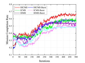
Figure 2: Convergence performance of the HICMS and existing algorithms.

VI-B Performance Evaluation

VI-B1 Performance Analysis of CMS

Figure 2 shows the convergence performance of the HICMS and existing algorithms. It can be seen that the mission completion rate (MCR) obtained by the HICMS during the training process fluctuates and rises with the optimization of the CMS policy and finally converges stably with small fluctuations. Furthermore, whether burst missions are generated, the HICMS has the best learning ability.

As shown in Figs. 3 and 4, we verify that the CMS leads to significant performance gains under common missions. Specifically, HICMS achieves higher MCR under different communication and energy resource configurations through efficiently collaborating the inter-domain resources (For example, the number of missions offloaded by $\mathcal{D}_{2}$ increases significantly and exceeds the total number of missions collected $\mathcal{D}_{2}$.). Further, with the increase of SGL transmission rate and battery capacity, the gain of CMS increases gradually. The reasons are: 1) the increase in transmission rate makes missions in each domain be offloaded in time to reduce storage occupancy rate, which improves the possibility of inter-domain resource collaboration; 2) CMS needs to consume more energy and the improvement of battery capacity provides more energy supply for CMS to improve mission offloading capability. Besides, IDMS can obtain gains under sufficient communication and energy resources through efficiently collaborating the intra-domain resources.

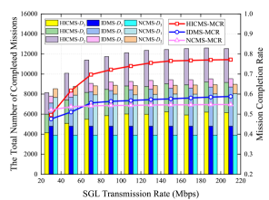
Figure 3: The total number of completed missions and MCR versus SGL transmission rate.

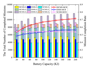
Figure 4: The total number of completed missions and MCR versus $E_{max}$.

Figures 5 and 6 show the number of completed common and burst missions under different the arrival rates of burst CMs and under different survival time slots of burst CMs to verify that the CMS can obtain better performance under burst missions. In Fig. 5, whether the arrival rate of burst missions is large or small, the total number of completed missions by the HICMS is the largest, and the total number of completed missions by the three algorithms gradually increases. In addition, with increasing the arrival rate of burst missions, the number of completed burst missions by the HICMS gradually increases and surpasses that of IDMS and NCMS. However, due to the highest priority of burst missions, the increase in burst missions makes the offloading of common missions lag, which reduces the number of completed common missions. In Fig. 6, with increasing the survival time slot of burst CMs, the number of completed burst missions by the three algorithms first increases and then stabilizes. Furthermore, the total number of completed missions by the HICMS is the largest. The reason is that the larger the survival time slot is, the more opportunities the burst missions have to be successfully offloaded. However, when the survival time slot is large, limited resources make it impossible for the number of completed missions to grow continuously. Furthermore, due to the long-term wait for burst missions to be transmitted, the number of completed common missions is reduced.

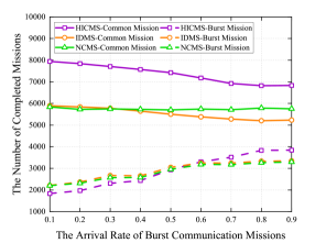
Figure 5: The number of completed missions versus the arrival rate of burst CMs.

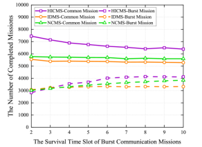
Figure 6: The number of completed missions versus the survival time slot of burst CMs.

Table II: Different algorithms’ performance under different the number of domains.

The number of domains	The total number of completed missions
	Common mission (Mode 1)					Common and burst missions (Mode 2)
	HICMS	IDMS	NCMS	ICMS	BTS	HICMS	IDMS	NCMS	ICMS	BTS
2 domains	5395	3977	4954	5370	2462	4838 (4002/836)	3591 (2844/747)	4396 (3577/819)	4426 (3464/962)	2405 (2078/327)
3 domains	10927	8718	8794	9167	6006	10367 (7150/3217)	8294 (5684/2610)	8150 (5924/2226)	9114 (5961/3153)	5326 (3965/1361)
4 domains	15398	13587	12700	14497	10161	14229 (10557/3672)	13125 (8689/4436)	11818 (8161/3657)	13714 (9436/4278)	8698 (6391/2307)
5 domains	20566	17338	15973	17040	11737	17070 (12701/4377)	15124 (10110/5014)	14101 (9746/4355)	15586 (11182/4404)	9953 (7476/2477)
6 domains	21071	18258	16824	18120	12583	18347 (13704/4643)	16641 (11576/5065)	15300 (10690/4610)	15607 (10953/4654)	11012 (8367/2645)

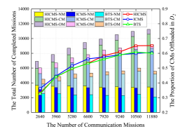
Figure 7: The total number of completed missions and the proportion of CMs offloaded in $\mathcal{D}_{2}$ under different the number of CMs.

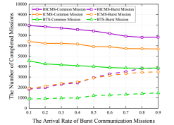
Figure 8: The number of completed missions versus the arrival rate of burst CMs.

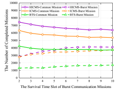
Figure 9: The number of completed missions versus the survival time slot of burst CMs.

VI-B2 Performance Comparisons of Different Cross-domain Algorithms

Figure 9 shows the total number of completed missions and the proportion of CMs offloaded in $\mathcal{D}_{2}$ under different the number of CMs. It can be seen that with increasing the number of CMs, the performance of the HICMS is better than the ICMS and BTS, and the total number of completed missions increases gradually. Furthermore, for the three algorithms, the increase of CMs does not affect the offloading of NMs, because the priority of NMs is higher than that of CMs. However, the number of offloaded OMs decreased gradually, which indicates that the significant increase in the number of offloaded CMs is assisted by $\mathcal{D}_{2}$. The proportion of CMs offloaded in $\mathcal{D}_{2}$ also effectively proves this conclusion. It can be observed from the curve that the proportion of CMs in the missions offloaded by $\mathcal{D}_{2}$ increases gradually, and the inter-domain collaboration performance of the HICMS is better. Besides, since ICMS directly selects intra-domain/inter-domain relays for cooperative mission scheduling and IDLs do not exist in every time slot, inter-domain collaboration performance and the number of completed missions are poorer than HICMS.

As shown in Figs. 9 and 9, whether common missions or burst missions, HICMS obtains the best performance, and the total number of completed missions gradually increases. In Fig. 9, when the arrival rate of burst missions is small, the number of completed burst missions of HICMS and ICMS is almost equal, and with the arrival rate of burst missions increasing, the performance of the HICMS outperforms that of the ICMS. The reason is that the inter-domain collaboration of ICMS is poor, and burst missions cannot be completed through efficient inter-domain resource collaboration when the intra-domain resources cannot be supplied in time. Besides, since BTS cannot effectively select the CMS policy based on resources and mission states, the total number of completed missions hardly increases. In Fig. 9, similarly, due to the difficulty in guaranteeing the effective offloading of burst missions, with increasing the survival time slot of burst CMs, the number of completed burst missions in ICMS increases slightly and soon stabilizes. The total number of completed missions remains almost unchanged for BTS.

VI-B3 Performance Comparisons under Different Network Scales

Table II shows the different algorithms’ performance comparison under different the number of domains. It can be observed that in Modes 1 and 2, the total number of completed missions by HICMS is the highest under different the number of domains. Furthermore, with increasing the number of domains, the total number of completed missions by the IDMS is similar to that of ICMS. The reason is that due to the poor inter-domain collaboration of the ICMS, the more domains, the harder it is to learn a better CMS policy to gradually loss the advantages of the CMS. In Mode 2, the number of completed common missions by the HICMS is always the highest, and the number of completed burst missions is not much different from the highest one. IDMS has a good performance for burst missions, which may be because burst missions with a higher priority can be directly offloaded in the domain to avoid the reduction of the remaining survival time slots. Besides, since the remaining survival time slots of burst missions are the smallest, under the same total number of missions, the number of completed missions in Mode 2 is less than in Mode 1.

Furthermore, it should be noted that due to limited transceivers of satellites, when the number of domains is greater than 3, we set that each domain selects only two domains as auxiliary domains and each CS establishes IDLs in the two auxiliary domains. Therefore, for the same number of domains, the MCR obtained by selecting different IDLs is also different, but the performance of HICMS is still higher than that of the other algorithms.

VII Conclusion

In this paper, we investigate the CMS problem for satellite networks to efficiently collaborate multi-domain resources. First, we accurately characterize the communication resource state of inter-satellite, and systematically characterize the differentiation of mission demands. Hereafter, we convert the CMS problem to the HCMS problem and develop the HICMS algorithm to solve it. The proposed algorithm can dynamically adjust and efficiently match the CMS policy to efficiently collaborate intra- and inter-domain resources to improve mission completion performance. Simulation results demonstrate that the proposed algorithm outperforms the independent domains and existing CMS algorithms and can still guarantee performance in case the network scales increase.

References

- [1] B. Deng, C. Jiang, H. Yao, S. Guo, and S. Zhao, “The next generation heterogeneous satellite communication networks: Integration of resource management and deep reinforcement learning,” IEEE Wireless Commun., vol. 27, no. 2, pp. 105–111, Apr. 2020.
- [2] H. Xie, Y. Zhan, G. Zeng, and X. Pan, “LEO mega-constellations for 6G global coverage: Challenges and opportunities,” IEEE Access, vol. 9, pp. 164 223–164 244, Dec. 2021.
- [3] P. Wang, B. Di, and L. Song, “Mega-constellation design for integrated satellite-terrestrial networks for global seamless connectivity,” IEEE Wireless Commun. Lett., vol. 11, no. 8, pp. 1669–1673, Aug. 2022.
- [4] M. Sheng, D. Zhou, W. Bai, J. Liu, H. Li, Y. Shi, and J. Li, “Coverage enhancement for 6G satellite-terrestrial integrated networks: performance metrics, constellation configuration and resource allocation,” Sci. China Inf. Sci., vol. 66, no. 3, pp. 1–20, Feb. 2023.
- [5] J. Radtke, C. Kebschull, and E. Stoll, “Interactions of the space debris environment with mega constellations - using the example of the OneWeb constellation,” Acta Astronaut., vol. 131, pp. 55–68, Feb. 2017.
- [6] T. Pultarova, “Telecommunications - space tycoons go head to head over mega satellite network [news briefing],” Eng. Technol., vol. 10, no. 2, p. 20, Mar. 2015.
- [7] Y. Su, Y. Liu, Y. Zhou, J. Yuan, H. Cao, and J. Shi, “Broadband LEO satellite communications: Architectures and key technologies,” IEEE Wireless Commun., vol. 26, no. 2, pp. 55–61, Apr. 2019.
- [8] W. Saad, M. Bennis, and M. Chen, “A vision of 6G wireless systems: Applications, trends, technologies, and open research problems,” IEEE Network, vol. 34, no. 3, pp. 134–142, May/June 2020.
- [9] J. A. Ruiz-de Azua, L. Fernandez, M. Badia, A. Marton, N. Garzaniti, A. Calveras, A. Golkar, and A. Camps, “Demonstration of the federated satellite systems concept for future earth observation satellite missions,” in Proc. IGARSS 2020, Waikoloa, HI, USA, Sept. 2020, pp. 3574–3577.
- [10] Q. Hao, M. Sheng, D. Zhou, and Y. Shi, “A multi-aspect expanded hypergraph enabled cross-domain resource management in satellite networks,” IEEE Trans. Commun., vol. 70, no. 7, pp. 4687–4701, July 2022.
- [11] H. He, D. Zhou, M. Sheng, and J. Li, “Hierarchical cross-domain satellite resource management: An intelligent collaboration perspective,” IEEE Trans. Commun., vol. 71, no. 4, pp. 2201–2215, Apr. 2023.
- [12] C.-Q. Dai, C. Li, S. Fu, J. Zhao, and Q. Chen, “Dynamic scheduling for emergency tasks in space data relay network,” IEEE Trans. Veh. Technol., vol. 70, no. 1, pp. 795–807, Jan. 2021.
- [13] A. Marahatta, S. Pirbhulal, F. Zhang, R. M. Parizi, K.-K. R. Choo, and Z. Liu, “Classification-based and energy-efficient dynamic task scheduling scheme for virtualized cloud data center,” IEEE Trans. Cloud Comput., vol. 9, no. 4, pp. 1376–1390, Oct.-Dec. 2021.
- [14] D. Zhou, M. Sheng, B. Li, J. Li, and Z. Han, “Distributionally robust planning for data delivery in distributed satellite cluster network,” IEEE Trans. Wireless Commun., vol. 18, no. 7, pp. 3642–3657, July 2019.
- [15] Q. Qi, L. Zhang, J. Wang, H. Sun, Z. Zhuang, J. Liao, and F. R. Yu, “Scalable parallel task scheduling for autonomous driving using multi-task deep reinforcement learning,” IEEE Trans. Veh. Technol., vol. 69, no. 11, pp. 13 861–13 874, Nov. 2020.
- [16] D. Zhou, M. Sheng, J. Li, and Z. Han, “Aerospace integrated networks innovation for empowering 6G: A survey and future challenges,” IEEE Commun. Surv. Tutorials, vol. 25, no. 2, pp. 975–1019, Feb. 2023.
- [17] D. Zhou, M. Sheng, R. Liu, Y. Wang, and J. Li, “Channel-aware mission scheduling in broadband data relay satellite networks,” IEEE J. Sel. Areas Commun., vol. 36, no. 5, pp. 1052–1064, May 2018.
- [18] L. Wang, C. Jiang, L. Kuang, S. Wu, H. Huang, and Y. Qian, “High-efficient resource allocation in data relay satellite systems with users behavior coordination,” IEEE Trans. Veh. Technol., vol. 67, no. 12, pp. 12 072–12 085, Dec. 2018.
- [19] P. Li, J. Li, H. Li, S. Zhang, and G. Yang, “Graph based task scheduling algorithm for earth observation satellites,” in Proc. IEEE GLOBECOM, Abu Dhabi, United Arab Emirates, Dec. 2018, pp. 1–7.
- [20] X. Chen, X. Li, X. Wang, Q. Luo, and G. Wu, “Task scheduling method for data relay satellite network considering breakpoint transmission,” IEEE Trans. Veh. Technol., vol. 70, no. 1, pp. 844–857, 2021.
- [21] G. Wu, Q. Luo, Y. Zhu, X. Chen, Y. Feng, and W. Pedrycz, “Flexible task scheduling in data relay satellite networks,” IEEE Trans. Aerosp. Electron. Syst., vol. 58, no. 2, pp. 1055–1068, Apr. 2022.
- [22] J. Wang, X. Zhu, D. Qiu, and L. T. Yang, “Dynamic scheduling for emergency tasks on distributed imaging satellites with task merging,” IEEE Trans. Parallel Distrib. Syst., vol. 25, no. 9, pp. 2275–2285, Sept. 2014.
- [23] S. Haiquan, X. Wei, H. Xiaoxuan, and X. Chongyan, “Earth observation satellite scheduling for emergency tasks,” J. Syst. Eng. Electron., vol. 30, no. 5, pp. 931–945, Oct. 2019.
- [24] Z. Liu and W. Xiong, “A DQN-based hyperheuristic algorithm for emergency scheduling of earth observation satellites,” in Proc. CECIT, Sanya, China, Dec. 2021, pp. 39–47.
- [25] B. Deng, C. Jiang, L. Kuang, S. Guo, N. Ge, and J. Lu, “Preemptive dynamic scheduling algorithm for data relay satellite systems,” in Proc. IEEE ICC, Paris, France, May 2017, pp. 1–6.
- [26] B. Deng, C. Jiang, L. Kuang, S. Guo, J. Lu, and S. Zhao, “Two-phase task scheduling in data relay satellite systems,” IEEE Trans. Veh. Technol., vol. 67, no. 2, pp. 1782–1793, Feb. 2018.
- [27] C. Bao, M. Sheng, D. Zhou, Y. Shi, and J. Li, “Towards intelligent cross-domain resource coordinate scheduling for satellite networks,” IEEE Trans. Wireless Commun., 2023, Early Access.
- [28] Q. Chen, G. Giambene, L. Yang, C. Fan, and X. Chen, “Analysis of inter-satellite link paths for LEO mega-constellation networks,” IEEE Trans. Veh. Technol., vol. 70, no. 3, pp. 2743–2755, Mar. 2021.
- [29] J. L. Laso Fernández, “Study, modelling and design of intersatellite links (ISL) in millimeter-wave band/estudio, modelado y diseño de enlaces intersatelitales (ISL) en bandas de milimétricas,” Telecomunicacion, July 2020.
- [30] D. Zhou, M. Sheng, J. Luo, R. Liu, J. Li, and Z. Han, “Collaborative data scheduling with joint forward and backward induction in small satellite networks,” IEEE Trans. Commun., vol. 67, no. 5, pp. 3443–3456, May 2019.
- [31] S. Fu, J. Gao, and L. Zhao, “Integrated resource management for terrestrial-satellite systems,” IEEE Trans. Veh. Technol., vol. 69, no. 3, pp. 3256–3266, Mar. 2020.
- [32] R. Liu, M. Sheng, K.-S. Lui, X. Wang, Y. Wang, and D. Zhou, “An analytical framework for resource-limited small satellite networks,” IEEE Commun. Lett., vol. 20, no. 2, pp. 388–391, Feb. 2016.
- [33] J. Wu, J. Zhang, J. Yang, and L. Xing, “Research on task priority model and algorithm for satellite scheduling problem,” IEEE Access, vol. 7, pp. 103 031–103 046, July 2019.
- [34] T. Chu, J. Wang, L. Codecà, and Z. Li, “Multi-agent deep reinforcement learning for large-scale traffic signal control,” IEEE Trans. Intell. Transp. Syst., vol. 21, no. 3, pp. 1086–1095, Mar. 2020.
- [35] Y. Zheng, J. Liu, M. Sheng, and C. Zhou, Exploiting Fingerprint Correlation for Fingerprint-Based Indoor Localization: A Deep Learning-Based Approach. Cham: Springer International Publishing, 2023, pp. 201–237.
- [36] A. M. Saxe, J. L. McClelland, and S. Ganguli, “Exact solutions to the nonlinear dynamics of learning in deep linear neural networks,” arXiv preprint arXiv:1312.6120, Dec. 2013.
- [37] A. Golkar and I. Lluch i Cruz, “The federated satellite systems paradigm: Concept and business case evaluation,” Acta Astronautica, vol. 111, pp. 230–248, June 2015.