Reliable Prediction Intervals with Regression Neural Networks

Abstract

This paper proposes an extension to conventional regression Neural Networks (NNs) for replacing the point predictions they produce with prediction intervals that satisfy a required level of confidence. Our approach follows a novel machine learning framework, called Conformal Prediction (CP), for assigning reliable confidence measures to predictions without assuming anything more than that the data are independent and identically distributed (i.i.d.). We evaluate the proposed method on four benchmark datasets and on the problem of predicting Total Electron Content (TEC), which is an important parameter in trans-ionospheric links; for the latter we use a dataset of more than 60000 TEC measurements collected over a period of 11 years. Our experimental results show that the prediction intervals produced by our method are both well-calibrated and tight enough to be useful in practice.

1 Introduction

Conformal Prediction (CP) is a novel framework for complementing the predictions of traditional machine learning algorithms with valid measures of their confidence. Confidence measures indicate the likelihood of each prediction being correct and therefore provide the ability of making much more informed decisions. This makes them a highly desirable feature of the techniques developed for many real-world applications.

In this paper we develop a regression CP based on Neural Networks (NNs), which is one of the most popular machine learning techniques. Some indicative fields in which NNs have been used with success are medicine, image processing, environmental modelling, robotics and the industry (see e.g. Mantzaris et al., 2008; Iliadis & Maris, 2007; Yang et al., 2009; Iliadis et al., 2008). In order to apply CP to NNs we follow a modified version of the original CP approach, called Inductive Conformal Prediction (ICP). ICP was proposed by Papadopoulos et al. (2002a) and Papadopoulos et al. (2002b) in an effort to overcome the computational inefficiency problem of CP. As demonstrated in the work of Papadopoulos (2008), which describes ICP and its application to classification NNs, this computational inefficiency problem renders the original CP approach highly unsuitable for being coupled with NNs; and in general any method that requires long training times.

In the case of regression, instead of the point predictions produced by conventional techniques, CPs produce prediction intervals that satisfy a given level of confidence. The important property of these intervals is that they are well-calibrated, meaning that in the long run the intervals produced for some confidence level $1-\delta$ will not contain the true label of an example with a relative frequency of at most $\delta$. Moreover, this is achieved without assuming anything more than that the data are independent and identically distributed (i.i.d.), which is the typical assumption of most machine learning methods.

We first evaluate the proposed method on four benchmark datasets from the UCI (Frank & Asuncion, 2010) and DELVE (Rasmussen et al., 1996) machine learning repositories. Then we apply it to the problem of predicting Total Electron Content (TEC), which is an important parameter that represents a quantitative measure of the detrimental effect of the ionosphere (an ionised region in the upper atmosphere) on electromagnetic signals from space-based systems propagating through it. Prediction of TEC enables mitigation techniques to be applied in order to reduce these undesirable ionospheric effects on radar, communication, surveillance and navigation signals. For this reason, the use of NNs for TEC prediction was addressed in many studies such as (Cander et al., 1998; Maruyama, 2007; Haralambous et al., 2010). In this work we make one step further and provide prediction intervals, which make mitigation techniques more effective as they allow taking into account the highest possible TEC value at a desired confidence level.

The rest of the paper starts with an overview of related work on CP, on the alternative ways of obtaining confidence information and on the prediction of TEC and other Space Weather parameters in Section 2. This is followed by a brief description of the general idea behind CP and ICP in Section 3, while Section 4 details the Nearest Neighbours Regression ICP algorithm and gives the definition of a new normalized nonconformity measure. In Section 5 the proposed method is evaluated experimentally on four benchmark datasets. Subsequently, Section 6, first describes the characteristics of TEC and the measurement data used in this study, while it then presents its experimental results. Finally, Section 7, gives the conclusions and future directions of this work.

2 Related Work

This section gives a synopsis of the work carried out on Conformal Prediction since it was first proposed, of the alternative ways that can be used for producing confidence information and their important drawbacks, and of the use of machine learning techniques for the prediction of parameters in ionospheric and generally Space Weather research.

2.1 Conformal Prediction

CP was initially proposed by Gammerman et al. (1998) and later greatly improved by Saunders et al. (1999). In these papers CP was applied to Support Vector Machines for classification. Soon it started being applied to other popular classification algorithms, such as k-Nearest Neighbours (Proedrou et al., 2002), Decision Trees and Evolutionary Algorithms (Lambrou et al., 2011). In the case of regression, where its application becomes more complicated, an initial attempt to apply it to Ridge Regression was made by Melluish et al. (1999), while soon after a much better version was proposed by Nouretdinov et al. (2001a). Slightly later it was also applied to k-Nearest Neighbours for Regression by Papadopoulos et al. (2008, 2011).

At the same time, work was being carried out on overcoming the computational inefficiency problem of CP, which was due to its transductive nature. After trying out some ways of improving the efficiency of the transductive CP, such as “competitive transduction” and “transduction with hashing”, a much more radical modification was made by moving to inductive inference. This modified version of CP, called Inductive Conformal Prediction (ICP) was proposed by Papadopoulos et al. (2002a) for regression and by Papadopoulos et al. (2002b) for classification. ICP has also been applied to Neural Networks for classification in the work of Papadopoulos (2008), where a computational complexity analysis showing that ICPs are as efficient as their underlying algorithms can be found.

To date CPs have been applied to a variety of problems, such as the early detection of ovarian cancer (Gammerman et al., 2008), the classification of leukaemia subtypes (Bellotti et al., 2005), the recognition of hypoxia electroencephalograms (EEGs) (Zhang et al., 2008), the prediction of plant promoters (Shahmuradov et al., 2005), the diagnosis of acute abdominal pain (Papadopoulos et al., 2009a), the assessment of stroke risk (Lambrou et al., 2010) and the estimation of effort for software projects (Papadopoulos et al., 2009b).

2.2 Alternative Ways of Producing Confidence Information

There are two other machine learning areas that can be used for producing some kind of confidence information; these are the Bayesian framework and the theory of Probably Approximately Correct learning (PAC theory, Valiant, 1984).

The Bayesian framework can be used for producing methods that complement individual predictions with probabilistic measures of their quality. These measures though, are based on some a priori assumptions about the distribution generating the data. If the correct prior is known, the measures produced by Bayesian methods are optimal. The problem is that for real world data the required knowledge is typically not available and as a result one is forced to assume the existence of some arbitrarily chosen prior. In this case, since the assumed prior is most probably violated, the outputs of Bayesian methods may become quite misleading. For example the prediction intervals output for the 95% confidence level may contain the true label in much less than 95% of the cases. This signifies a major failure, as we would expect confidence levels to bound the percentage of expected errors. Papadopoulos et al. (2011) demonstrate experimentally this negative aspect of Bayesian techniques by applying Gaussian Process Regression (Rasmussen & Williams, 2006) to three benchmark datasets. A more detailed experimental comparison of Bayesian techniques and CP, that resulted in the same conclusion, for both classification and regression was performed by Melluish et al. (2001).

On the other hand, PAC theory can be applied to an algorithm in order to produce upper bounds on the probability of its error with respect to some confidence level. Contrary to Bayesian techniques, PAC theory only assumes that the data are generated independently by some completely unknown distribution. In order for the bounds produced by PAC theory to be interesting in practice however, the dataset in question should be particularly clean. As this is rarely the case, the resulting bounds are typically very loose and therefore not very useful in practice. A demonstration of the crudeness of PAC bounds was performed by Nouretdinov et al. (2001b). Furthermore, PAC theory has two additional drawbacks: (a) the majority of relevant results either involve large explicit constants or do not specify the relevant constants at all; (b) the bounds obtained by PAC theory are for the overall error and not for individual predictions.

All above problems are overcome by CPs, which in contrast to Bayesian techniques produce well-calibrated outputs as they are only based on the general i.i.d. assumption. Moreover, unlike PAC theory, they produce confidence measures that are useful in practice and are associated with individual predictions. Both the robustness of the resulting prediction intervals and their usefulness are demonstrated experimentally for the proposed methods in Sections 5 and 6.2.

2.3 Space Weather Parameter Prediction

Machine learning techniques have been applied widely in the last $18$ years for the specification, long-term prediction and short-term forecasting of Space Weather parameters and particularly ionospheric related parameters. The non-linear nature of a vast array of phenomena affecting the state and variability of Space Weather and the upper atmosphere within the whole chain of Solar Terrestrial effects represents a challenging field for the application of such techniques (Lundstedt, 1992).

Starting from the principal driver of Space Weather, solar activity, neural networks have been used to provide a functional representation of its benign state (Macpherson, 1993; Gleisner & Lundstedt, 2001). In addition to neural networks, Support Vector Machines (Gavrishchaka & Ganguli, 2001), Time-Delay Neural Networks (Gleisner et al., 1996) and Elman Recurrent Neural Networks (Wu & Lundstedt, 1996) have been applied to predict geomagnetic disturbances which are essentially short time scale consequence effects specific to solar activity transient phenomena. The nature and general morphology of these phenomena is very complex to model from first principles due to the numerous interactions involving various atmospheric layers.

A number of studies have also been conducted concentrating on the prediction of TEC and other related ionospheric parameters important for telecommunication applications. These studies have dealt with short-term forecasting (Cander et al., 2003; Liu et al., 2005; Koutroumbas et al., 2008; Strangeways et al., 2009; Stamper et al., 2004) and long-term prediction (Maruyama, 2007; Haralambous et al., 2010; Agapitos et al., 2010) of such parameters as well as coping with missing data points (Francis et al., 2001). Furthermore, it is important to note that work in this area is not limited to temporal variations of parameters, it also includes spatial ones (Oyeyemi & Poole, 2004).

3 The Conformal Prediction Framework

This section gives a brief description of the CP framework and its inductive version which is followed in this paper, for more details the interested reader is referred to the book by Vovk et al. (2005). We are interested in making a prediction for the label of an example $x_{l+g}$, based on a set of training examples $\{(x_{1},y_{1}),\dots,(x_{l},y_{l})\}$, where each $x_{i}\in\mathbb{R}^{d}$ is the vector of attributes for example $i$ and $y_{i}\in\mathbb{R}$ is the label of that example. Our only assumption is that all $(x_{i},y_{i})$, $i=1,2,\dots,$ have been generated independently from the same probability distribution (i.i.d.).

The idea behind CP is to assume every possible label $\tilde{y}$ of the example $x_{l+g}$ and check how likely it is that the extended set of examples

$$\{(x_{1},y_{1}),\dots,(x_{l},y_{l}),(x_{l+g},\tilde{y})\}$$ (1)

is i.i.d. This in effect will correspond to the likelihood of $\tilde{y}$ being the true label of the example $x_{l+g}$ since this is the only unknown value in (1).

To do this we first assign a value $\alpha^{\tilde{y}}_{i}$ to each pair $(x_{i},y_{i})$ in (1) which indicates how strange, or nonconforming, this pair is for the rest of the examples in the same set. This value, called the nonconformity score of the pair $(x_{i},y_{i})$, is calculated using a traditional machine learning algorithm, called the underlying algorithm of the corresponding CP. More specifically, we train the underlying algorithm on (1) and generate the prediction rule

$$D_{\{(x_{1},y_{1}),\dots,(x_{l},y_{l}),(x_{l+g},\tilde{y})\}},$$ (2)

which maps any input pattern $x_{i}$ to a predicted label $\hat{y}_{i}$. The nonconformity score of each pair $(x_{i},y_{i}):y=1,\dots,l,l+g$ is then measured as the degree of disagreement between the prediction

$$\hat{y}_{i}=D_{\{(x_{1},y_{1}),\dots,(x_{l},y_{l}),(x_{l+g},\tilde{y})\}}(x_{i})$$ (3)

and the actual label $y_{i}$; note that in the case of the pair $(x_{l+g},\tilde{y})$ the actual label is replaced by the assumed label $\tilde{y}$. The function used for measuring this degree of disagreement is called the nonconformity measure of the CP. Notice that a change in the assumed label $\tilde{y}$ affects all predictions (3) since it is part of the underlying algorithm’s training set.

The nonconformity score $\alpha^{\tilde{y}}_{l+g}$ is then compared to the nonconformity scores of all other examples to find out how unusual the pair $(x_{l+g},\tilde{y})$ is according to the nonconformity measure used. This comparison is performed with the function

$$p(\{(x_{1},y_{1}),\dots,(x_{l},y_{l}),(x_{l+g},\tilde{y})\})=\frac{\#\{i=1,\dots,l,l+g:\alpha^{\tilde{y}}_{i}\geq\alpha^{\tilde{y}}_{l+g}\}}{l+1},$$ (4)

which calculates the portion of examples in (1) that are equally or more nonconforming than $(x_{l+g},\tilde{y})$. The output of this function, which lies between $\frac{1}{l+1}$ and 1, is called the p-value of $\tilde{y}$, also denoted as $p(\tilde{y})$. An important property of (4) is that $\forall\delta\in[0,1]$ and for all probability distributions $P$ on $Z$,

$$P\{\{(x_{1},y_{1}),\dots,(x_{l},y_{l}),(x_{l+g},y_{l+g})\}:p(y_{l+g})\leq\delta\}\leq\delta,$$ (5)

in other words for i.i.d. data, the probability of the p-value for the true label $y_{l+g}$ being less than or equal to any given threshold $\delta$ is less than or equal to $\delta$; a proof can be found in the book by Vovk et al. (2005). This makes it a valid test of randomness with respect to the i.i.d. model. According to this property, if $p(\tilde{y})$ is under some very low threshold, say $0.05$, this means that $\tilde{y}$ is highly unlikely of being the true label as the probability of such an event is at most $5\%$ if (1) is i.i.d.

Assuming it were possible to calculate the p-value of every possible label following the above procedure, we could then exclude all labels with a p-value under some very low threshold, or significance level, $\delta$ and have at most $\delta$ chance of being wrong. Consequently, given a confidence level $1-\delta$ a regression CP outputs the set

$$\{\tilde{y}:p(\tilde{y})>\delta\},$$ (6)

in other words the interval containing all labels that have a p-value greater than $\delta$. Of course it is impossible to explicitly consider every possible label $\tilde{y}\in\mathbb{R}$, so regression CPs follow a different approach which makes it possible to compute the prediction interval (6). This approach is described by Nouretdinov et al. (2001a) for Ridge Regression and by Papadopoulos et al. (2008) for $k$-Nearest Neighbours Regression.

3.1 Inductive Conformal Prediction

The only drawback of the original CP approach is that due to its transductive nature all its computations, including training the underlying algorithm, have to be repeated for each assumed label of every new test example. This makes it very computationally inefficient especially for algorithms that require long training times such as NNs. Furthermore, in the case of regression where it is impossible to explicitly consider every possible label of the new example, the approach followed by Nouretdinov et al. (2001a) and Papadopoulos et al. (2008) for computing the prediction interval (6) can only be employed if it is possible to calculate how a change in $\tilde{y}$ will affect the predictions produced by (3) for all examples in (1) and consequently the resulting nonconformity scores $\alpha^{\tilde{y}}_{1},\dots,\alpha^{\tilde{y}}_{l},\alpha^{\tilde{y}}_{l+g}$. ICP is based on the same theoretical foundations described above, but performs inductive rather than transductive inference. As a result ICP is almost as efficient as its underlying algorithm (Papadopoulos, 2008) and it can be combined with any conventional regression method.

ICP splits the training set (of size $l$) into two smaller sets, the proper training set with $m<l$ examples and the calibration set with $q:=l-m$ examples. It then uses the proper training set for training its underlying algorithm and the calibration set for calculating the p-value of each possible label $\tilde{y}$. More specifically, it trains the underlying algorithm on $(x_{1},y_{1}),\dots,(x_{m},y_{m})$ to generate the prediction rule

$$D_{\{(x_{1},y_{1}),\dots,(x_{m},y_{m})\}},$$ (7)

and calculates the nonconformity score $\alpha_{m+i}$ of each example in the calibration set $(x_{m+i},y_{m+i}),i=1,\dots,q$ as the degree of disagreement between the prediction

$$\hat{y}_{m+i}=D_{\{(x_{1},y_{1}),\dots,(x_{m},y_{m})\}}(x_{m+i})$$ (8)

and the actual label $y_{m+i}$. This needs to be done only once as now $x_{l+g}$ is not included in the training set of the underlying algorithm. From this point on, it only needs to compute the prediction

$$\hat{y}_{l+g}=D_{\{(x_{1},y_{1}),\dots,(x_{m},y_{m})\}}(x_{l+g})$$ (9)

for each new example $x_{l+g}$ and calculate the nonconformity score $a^{\tilde{y}}_{l+g}$ of the pair $(x_{l+g},\tilde{y})$ for every possible label $\tilde{y}$ as the degree of disagreement between itself the prediction $\hat{y}_{l+g}$. The p-value of $\tilde{y}$ can now be calculated as

$$p(\tilde{y})=\frac{\#\{i=m+1,\dots,m+q,l+g:\alpha_{i}\geq\alpha^{\tilde{y}}_{l+g}\}}{q+1}.$$ (10)

Again it is impossible to explicitly go through every possible label $\tilde{y}\in\mathbb{R}$ to calculate its p-value, but it is possible to compute the prediction interval (6) as we show in the next section.

4 Neural Networks Regression ICP

In order to use ICP in conjunction with some traditional algorithm we first have to define a nonconformity measure. Recall that a nonconformity measure is a function that measures the disagreement between the actual label $y_{i}$ and the prediction $\hat{y}_{i}$ produced by the prediction rule (7) of the underlying algorithm for the example $x_{i}$. In the case of regression this can be easily defined as the absolute difference between the two

$$\alpha_{i}=|y_{i}-\hat{y}_{i}|.$$ (11)

We first describe the Neural Networks Regression ICP (NNR ICP) algorithm with this measure and then define a normalized nonconformity measure, which has the effect of producing tighter prediction intervals by taking into account the expected accuracy of the underlying NN on each example.

The first steps of the NNR ICP algorithm follow exactly the general scheme given in Section 3.1:

• Split the training set $\{(x_{1},y_{1}),\dots,(x_{l},y_{l})\}$ into two subsets:

  • the proper training set: $\{(x_{1},y_{1}),\dots,(x_{m},y_{m})\}$, and

  • the calibration set: $\{(x_{m+1},y_{m+1}),\dots,(x_{m+q},y_{m+q})\}$.

• Use the proper training set to train the NN.

• For each pair $(x_{m+i},y_{m+i}),i=1,\dots,q$ in the calibration set:

  • supply the input pattern $x_{m+i}$ to the trained NN to obtain the prediction $\hat{y}_{m+i}$ and

  • calculate the nonconformity score $\alpha_{m+i}$ with (11).

At this point however, it becomes impossible to follow the general ICP scheme as there is no way of trying out all possible labels $\tilde{y}\in\mathbb{R}$ in order to calculate their nonconformity score and p-value. Notice though that both the nonconformity scores of the calibration set examples $\alpha_{m+1},\dots,\alpha_{m+q}$ and the prediction $\hat{y}_{l+g}$ of the trained NN for the new example $x_{l+g}$ will remain fixed as we change the assumed label $\tilde{y}$. The only value that will change is the nonconformity score

$$\alpha^{\tilde{y}}_{l+g}=|\tilde{y}-\hat{y}_{l+g}|.$$ (12)

Thus $p(\tilde{y})$ will only change at the points where $\alpha^{\tilde{y}}_{l+g}=\alpha_{m+i}$ for some $i=1,\dots,q$. As a result, for a given confidence level $1-\delta$ we only need to find the biggest $\alpha_{m+i}$ such that when $\alpha^{\tilde{y}}_{l+g}=\alpha_{m+i}$ then $p(\tilde{y})>\delta$, which will give us the maximum and minimum $\tilde{y}$ that have a p-value greater than $\delta$ and consequently the beginning and end of the corresponding prediction interval. More specifically, after calculating the nonconformity scores of all calibration examples the NNR ICP algorithm continues as follows:

• Sort the nonconformity scores of the calibration examples in descending order obtaining the sequence

  $$\alpha_{(m+1)},\dots,\alpha_{(m+q)}.$$ (13)

• For each new test example $x_{l+g}$:

  • supply the input pattern $x_{l+g}$ to the trained NN to obtain the prediction $\hat{y}_{l+g}$ and

  • output the prediction interval

    $$(\hat{y}_{l+g}-\alpha_{(m+s)},\hat{y}_{l+g}+\alpha_{(m+s)}),$$ (14)

    where

    $$s=\lfloor\delta(q+1)\rfloor.$$ (15)

An important parameter of the ICP algorithm is the number $q$ of training examples that will be allocated to the calibration set and the nonconformity scores of which will be used by the ICP to generate its prediction intervals. This number should only correspond to a small portion of the training set, as in the opposite case the removal of these examples will result in a significant reduction to the predictive ability of the underlying NN and consequently to wider than desirable prediction intervals. As we are mainly interested in the confidence levels of $99\%$ and $95\%$, the calibration sizes we use are of the form $q=100n-1$, where $n\in{{{\mathbb{N}}}}$ (see (15)).

4.1 A Normalized Nonconformity Measure

We extend nonconformity measure definition (11) by normalizing it with the predicted accuracy of the underlying NN on the given example. This leads to prediction intervals that are larger for the “difficult” examples and smaller for the “easy” ones. As a result the ICP can satisfy the required confidence level with intervals that are on average tighter.

Our new measure is defined as

$$\alpha_{i}=\frac{|y_{i}-\hat{y}_{i}|}{\exp(\mu_{i})+\beta},$$ (16)

where $\mu_{i}$ is the prediction of the value $\ln(|y_{i}-\hat{y}_{i}|)$ produced by a linear NN trained on the proper training patterns and $\exp$ is the exponential function. In effect after training the underlying NN of the ICP we calculate the residuals $|y_{j}-\hat{y}_{j}|$ for all proper training examples $j=1,\dots,m$ and train a linear NN on the pairs $(x_{j},\ln(|y_{j}-\hat{y}_{j}|))$ producing the prediction rule

$$D_{\{(x_{1},\ln(|y_{1}-\hat{y}_{1}|)),\dots,(x_{m},\ln(|y_{m}-\hat{y}_{m}|))\}}.$$ (17)

Then $\mu_{i}$ is the prediction

$$\mu_{i}=D_{\{(x_{1},\ln(|y_{1}-\hat{y}_{1}|)),\dots,(x_{m},\ln(|y_{m}-\hat{y}_{m}|))\}}(x_{i}).$$ (18)

of this linear NN for the input pattern $x_{i}$. The parameter $\beta\geq 0$ controls the sensitivity of the measure to changes of $\mu_{i}$, since the latter depends on the range of possible labels and the complexity of the problem in question.

We use a linear rather than a more complex NN as we want the prediction rule (17) to capture only the important variation of the loss of the underlying NN and not be affected by small changes, which are mainly due to noise. Besides linear NN are much faster to train, which means that the computational efficiency of the ICP is not affected by much. We also use the logarithmic instead of the direct scale to ensure that the estimate is always positive.

When using (16) as nonconformity measure the prediction interval produced by the ICP for each new pattern $x_{l+g}$ becomes

$$(\hat{y}_{l+g}-\alpha_{(m+s)}(\exp(\mu_{l+g})+\beta),\hat{y}_{l+g}+\alpha_{(m+s)}(\exp(\mu_{l+g})+\beta)),$$ (19)

where again $s=\lfloor\delta(q+1)\rfloor$.

5 Experimental Evaluation on Benchmark Datasets

We tested the proposed method on four benchmark datasets from the UCI (Frank & Asuncion, 2010) and DELVE (Rasmussen et al., 1996) repositories:

• Boston Housing, which lists the median house prices for $506$ different areas of Boston MA in $1000s. Each area is described by 13 attributes such as pollution and crime rate.

• Abalone, which concerns the prediction of the age of abalone from physical measurements. The data set consists of 4177 examples described by 8 attributes such as diameter, height and shell weight.

• Computer Activity, which is a collection of a computer systems activity measures from a Sun SPARCstation 20/712 with 128 Mbytes of memory running in a multi-user university department. It consists of 8192 examples of 12 measured values, such as the number of system buffer reads per second and the number of system call writes per second, at random points in time. The task is to predict the portion of time that the cpus run in user mode, ranging from 0 to 100. We used the small variant of the data set which contains only 12 of the 21 attributes.

• Bank, which was generated from simplistic simulator of the queues in a series of banks. The task is to predict the rate of rejections, i.e. the fraction of customers that are turned away from the bank because all the open tellers have full queues. The data set consists of 8192 examples described by 8 attributes like area population size and maximum possible length of queues. We used the 8nm variant of the data set which contains 8 of the 32 attributes, and is highly non-linear with moderate noise.

Before conducting our experiments the attributes of all datasets were normalized to a minimum value of -1 and a maximum value of 1. Our experiments followed a fold cross-validation process; each dataset was split randomly into $k$ folds of almost equal size and our experiments were repeated $k$ times each time using one of the $k$ folds as test set and the other $k-1$ folds as training set. In order to ensure that the results reported here do not depend on the particular split of the dataset into the $k$ folds or in the particular choice of calibration examples, this process was repeated 10 times with different permutations of the examples. Based on their sizes the Boston Housing and Abalone datasets were split into 10 and 4 folds respectively, while the other two were splint into 2 folds. The calibration set sizes were set to $q=100n-1$ (see Section 4), where $n$ was chosen so that $q$ was approximately $1/10$th of each dataset’s training size; in the case of the Boston Housing data set the smallest value $n=1$ was used due to its small size.

	Boston		Computer
	Housing	Abalone	Activity	Bank
Examples	506	4177	8192	8192
Attributes	13	8	12	8
Label range	45	28	99	0.48
Folds	10	4	2	2
Hidden Neurons	7	8	17	13
Calibration size	99	299	399	399

Table 1: Main characteristics and experimental setup for each data set.

		Original NNR				NNR ICP
		RMSE		CC		RMSE		CC
Boston Housing		4.059		0.900		4.307		0.885
Abalone		2.091		0.761		2.099		0.759
Computer Activity		3.105		0.986		3.249		0.984
Bank		0.019		0.953		0.019		0.950

Table 2: Point prediction performance of NNR ICP and its underlying Neural Network.

				Interdecile			Percentage
Nonconformity	Median Width			Mean Width			of Errors (%)
Measure	90%	95%	99%	90%	95%	99%	90%	95%	99%
(11)	12.44	17.18	39.32	12.49	17.07	38.68	10.18	4.66	0.87
(16) - $\beta=0$	11.93	16.82	35.81	12.48	17.67	39.91	10.26	5.02	1.09
(16) - $\beta=0.5$	11.67	16.13	32.19	12.03	16.74	34.94	10.16	4.94	1.03

Table 3: Tightness and empirical reliability results for the Boston Housing Dataset.

				Interdecile			Percentage
Nonconformity	Median Width			Mean Width			of Errors (%)
Measure	90%	95%	99%	90%	95%	99%	90%	95%	99%
(11)	6.60	9.08	14.97	6.64	9.07	14.89	10.01	5.02	0.91
(16) - $\beta=0$	5.48	7.31	12.69	5.73	7.63	13.28	9.86	4.89	0.85
(16) - $\beta=0.5$	5.65	7.41	12.47	5.80	7.59	12.78	10.02	5.00	0.88

Table 4: Tightness and empirical reliability results for the Abalone Dataset.

				Interdecile			Percentage
Nonconformity	Median Width			Mean Width			of Errors (%)
Measure	90%	95%	99%	90%	95%	99%	90%	95%	99%
(11)	9.75	12.34	19.86	9.76	12.46	20.35	10.02	5.32	1.01
(16) - $\beta=0$	8.81	11.01	17.94	8.98	11.21	18.44	10.24	5.43	1.13
(16) - $\beta=0.5$	8.78	10.97	17.28	8.90	11.12	17.59	10.18	5.35	1.00

Table 5: Tightness and empirical reliability results for the Computer Activity Dataset.

				Interdecile			Percentage
Nonconformity	Median Width			Mean Width			of Errors (%)
Measure	90%	95%	99%	90%	95%	99%	90%	95%	99%
(11)	0.059	0.084	0.137	0.058	0.083	0.144	10.21	4.86	1.07
(16) - $\beta=0$	0.038	0.048	0.078	0.042	0.053	0.087	9.96	5.16	1.05
(16) - $\beta=0.5$	0.058	0.083	0.136	0.058	0.083	0.139	10.18	4.83	1.06

Table 6: Tightness and empirical reliability results for the Bank Dataset.

The underlying NN had a fully connected two-layer structure. The hidden layer consisted of neurons with hyperbolic tangent activation functions, while the output layer consisted of a single neuron with a linear activation function. The number of hidden neurons was determined by trial and error by performing a fold cross-validation process with the original NN predictor on 10 different random permutations than the ones used for evaluating the ICP. The training algorithm used was the Levenberg-Marquardt backpropagation algorithm with early stopping based on a validation set created from 10% of the proper training examples. In an effort to avoid local minima 10 NNs were trained with different random initialisations and the one that performed best on the validation set was selected for being applied to the calibration and test examples.

The number of examples and attributes of each dataset and the width of its range of labels, together with the number of folds $k$, calibration set size $q$ and number of hidden units used in our experiments are reported in Table 1. In the case of nonconformity measure (16) we experimented with $\beta=0$ and $\beta=0.5$ for all datasets to explore the difference that the addition of this parameter makes. It is worth to note however, that somewhat tighter prediction intervals can be obtained by adjusting $\beta$ for each dataset. We chose not to do this here so as to show that the huge improvement in prediction interval widths resulting from the use of this nonconformity measure does not depend on fine tuning this parameter.

Table 2 reports the performance of the point predictions of our method in terms of its Root Mean Squared Error (RMSE) and the Correlation Coefficient (CC) between the predicted and actual values and compares them to those of its underlying NN. This table basically shows the effect that the removal of the calibration examples has on the performance of the NN, since this is the only difference between the two as far as point predictions are concerned. The values presented in this table show that the performance decrease is not significant. This is a small prise that we have to pay for the much more informative outputs of the ICP.

Since the advantage of our method is that it produces prediction intervals, the main aim of our experiments was to check their tightness, and therefore usefulness, and their empirical reliability. To this end the first two parts of Tables 3-6 report the median and interdecile mean widths of the prediction intervals produced for the four datasets when using nonconformity measures (11) and (16) with $\beta$ set to $0$ and $0.5$ for the $90\%$, $95\%$ and $99\%$ confidence levels. We chose to report the median and interdecile mean values instead of the mean for evaluating prediction interval tightness so as to avoid the strong impact of a few extremely large or extremely small intervals. The third and last part of Tables 3-6 reports the percentage of errors made each time, which is in fact the percentage of intervals that did not contain the true label of the example.

More information on the tightness of the obtained prediction intervals are given in Figure 1, which shows the median, upper and lower quartiles, and upper and lower deciles of their widths for each dataset. Each chart is divided into three parts, one for each confidence level we consider, and each part contains a boxplot for each nonconformity measure used.

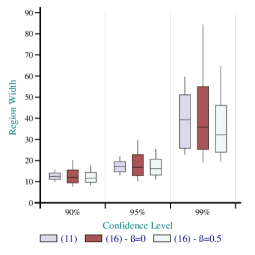
(a) Boston Housing

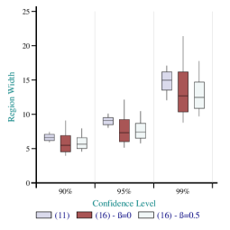
(b) Abalone

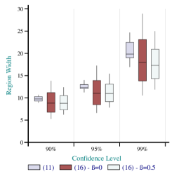
(c) Computer Activity

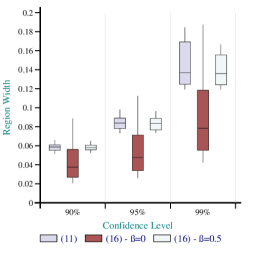
(d) Bank

Figure 1: Prediction interval width distribution for each dataset.

The values reported in Tables 3-6 in conjunction with the range of possible labels of each dataset show that the prediction intervals produced by our method are quite tight. For a confidence level as high as $99\%$ the median widths obtained with nonconformity measure (11) are $87.4\%$, $53.5\%$, $20.1\%$ and $28.5\%$ of the label range of the four datasets respectively, while the best widths obtained with nonconformity measure (16) are $71.5\%$, $44.5\%$, $17.5\%$ and $16.3\%$ of the label range. If we now consider the slightly lower $95\%$ confidence level the median widths obtained with nonconformity measure (11) are $38.2\%$, $32.4\%$, $12.5\%$ and $17.5\%$ of the label ranges respectively, while the best widths obtained with nonconformity measure (16) are $35.8\%$, $26.1\%$, $11.1\%$ and $10\%$ of the label ranges. It is worth to note that the relatively big intervals obtained for the Boston Housing dataset at the $99\%$ confidence level are partly due to the small size of the calibration set used in this case; this is also the reason for which these intervals become much tighter at the $95\%$ confidence level. Figure 1 shows the difference between the two nonconformity measures and demonstrates the improvement achieved by our normalized nonconformity measure (16). With the exception of the Boston Housing dataset, in all other cases more than half of the intervals of measure (16) are tighter than the 25th percentile of the widths produced by measure (11). In the case of the Bank dataset the difference is even more impressive. The same figure also shows the difference between the two values of $\beta$. When $\beta$ is set to $0$ the width distribution is bigger as the measure is more sensitive. When we slightly increase $\beta$ the sizes of the widths fluctuate less and in most cases become generally a bit smaller. In the case of the Bank dataset the value of $\beta=0.5$ was clearly too large considering that the label range of the dataset was smaller than $0.5$.

Finally, the values reported in the rightmost part of Tables 3-6 demonstrate the reliability of the obtained prediction intervals. The percentages reported in this part of the four tables are in all cases very near the required significance levels.

6 Total Electron Content Prediction

6.1 Characteristics and Measurement Data

TEC is defined as the total amount of electrons along a particular line of sight in the ionosphere and is measured in total electron content units (1 TECu = $10^{16}$ el/m²). It is an important parameter in trans-ionospheric links since when multiplied by a factor which is a function of the signal frequency, it yields an estimate of the delay imposed on the signal by the ionosphere (an ionized region ranging in height above the surface of the earth from approximately 50 to 1000 km) due to its dispersive nature (Kersley et al., 2004). The necessity for accurate prediction of TEC stems out of the fact that up to date and accurate information is needed in the application of mitigation techniques for the reduction of ionospheric imposed errors on radar, communication, surveillance and navigation systems.

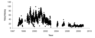
(a) Noon values of TEC

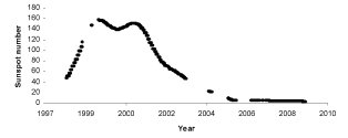
(b) Modelled monthly mean sunspot number

Figure 2: Long-term variability of TEC and solar activity.

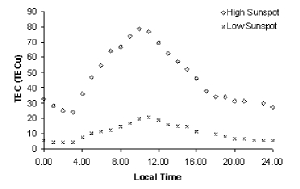
(a) 24-hour variability

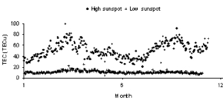
(b) Seasonal variability

Figure 3: 24-hour and seasonal variability of TEC for low and high solar activity.

The density of free electrons within the ionosphere and therefore TEC depend upon the strength of the solar ionizing radiation which is a function of time of day, season, geographical location and solar activity (Goodman, 1992). The long-term effect of solar activity on TEC follows an eleven-year cycle and is shown in Figure 2 where noon values of TEC are plotted against time as well as a modelled monthly mean sunspot number (R), which is a well established index of solar activity. Comparing the two we can observe a clear correlation between the mean level of TEC and the modelled sunspot number. We should note that during the last couple of years solar activity was characterised by a prolonged period of low sunspot values (see Figure 2). This however does not pose a problem to the approach adopted in this paper as the cyclic variation of solar activity is not embedded in the model specification. The 24-hour variability of TEC is demonstrated with two examples recorded during low and high solar activity in Figure 3a. Examples of its seasonal variability are shown in Figure 3b, in which the noon values of TEC are plotted again for low and high sunspot. As can be observed from these figures solar activity has an important effect on both the 24-hour and seasonal variability of TEC.

The TEC measurements used in this work consist of a bit more than 60000 values recorded between 1998 and 2009. The parameters used as inputs for modelling TEC are the hour, day and monthly mean sunspot number. The first two were converted into their quadrature components in order to avoid their unrealistic discontinuity at the midnight and change of year boundaries. Therefore the following four values were used in their place:

$$sinhour={{{{{{{{{\rm sin}}}}}}}}}(2\pi\frac{hour}{24}),$$ (20)

$$coshour={{{{{{{{{\rm cos}}}}}}}}}(2\pi\frac{hour}{24}),$$ (21)

$$sinday={{{{{{{{{\rm sin}}}}}}}}}(2\pi\frac{day}{365}),$$ (22)

$$cosday={{{{{{{{{\rm cos}}}}}}}}}(2\pi\frac{day}{365}).$$ (23)

It is worth to note that in ionospheric work solar activity is usually represented by the 12-month smoothed sunspot number, which however has the disadvantage that the most recent value available corresponds to TEC measurements made six months ago. In our case in order to enable TEC data to be modelled as soon as they are measured, and for future predictions of TEC to be made, the monthly mean sunspot number values were modelled using a smooth curve defined by a summation of sinusoids.

6.2 Experiments and Results

Our experiments followed the same experimental setting described in Section 5. Before conducting our experiments all attributes of the dataset were normalized to a minimum value of $-1$ and a maximum value of $1$. A 2-fold cross-validation process was performed 10 times on random permutations of the dataset with the 2 folds consisting of 30211 and 30210 examples respectively. This allowed the evaluation of the proposed method on the whole range of possible sunspot values (which typically exhibit an 11 year cycle), since solar activity has a strong effect on the variability of TEC. The calibration set size was set to $999$ examples, which resulted in $q+1$ in (15) being $1000$.

The underlying NN had the same structure and followed the same training process as the one used in the experiments of Section 5. In this case the number of hidden neurons was set to 13, which was as before determined by trial and error. Finally, for nonconformity measure (16) we again experimented with $\beta=0$ and $\beta=0.5$.

				Interdecile			Percentage
Nonconformity	Median Width			Mean Width			of Errors (%)
Measure	90%	95%	99%	90%	95%	99%	90%	95%	99%
(11)	16.15	21.88	38.17	16.32	22.02	38.67	10.12	5.02	1.01
(16) - $\beta=0$	13.04	16.24	25.91	14.20	17.69	28.27	9.73	4.92	1.00
(16) - $\beta=0.5$	12.90	16.17	26.81	13.82	17.33	28.70	9.82	4.96	0.97

Table 7: Tightness and empirical reliability results.

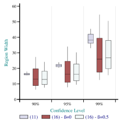
Figure 4: Prediction interval width distribution.

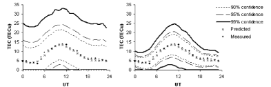
(a) Low Sunspot

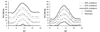
(b) Medium Sunspot

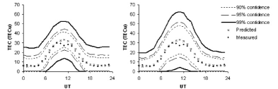
(c) High Sunspot

Figure 5: Examples of the prediction intervals produced by nonconformity measure (11) on the left and (16) on the right for typical days in low, medium and high sunspot periods.

In terms of point predictions both our method and the original NN performed quite well with a RMSE of $5.5$ TECu and a correlation coefficient between the predicted and the actual values of $0.94$; there was almost no difference between the two due to the large size of the dataset. The results of our method in terms of prediction interval tightness and empirical reliability are presented in Table 7, while boxplots showing the distribution of the obtained prediction interval widths are displayed in Figure 4. By considering the range of the measured values in our dataset, which are between $0$ and $110$ TECu, we can see that the prediction interval widths produced by the proposed method are quite impressive. For example, the median width obtained with nonconformity measure (16) and $\beta=0$ for the $99\%$ confidence level covers only $23.5\%$ of this range, while for the $95\%$ confidence level it covers $14.8\%$. It is worth to mention that, since the produced intervals are generated based on the size of the absolute error that the underlying algorithm can have on each example, a few of the intervals start from values below zero, which are impossible for the particular application. So we could in fact make these intervals start at zero without making any additional errors and this would result in slightly smaller values than those reported in this table. We chose not to do so here in order to evaluate the actual intervals as output by our method without any intervention. The error percentages reported in Table 7 again demonstrate the reliability of the obtained intervals as they are almost equal to the required significance level in all cases.

By comparing the boxplots presented in Figure 4 for each of the two nonconformity measures we can see the remarkable improvement that the normalized nonconformity measure (16) achieves. The majority of the prediction interval widths produced by measure (16) are below the 10th percentile of those produced by measure (11). The difference between the two measures is further demonstrated in Figure 5, which plots the intervals obtained by each measure for three typical days in the low, medium and high sunspot periods. Here we can see that unlike the intervals of measure (11), those of measure (16) are wider at noon and in the high sunspot period, when the variability of TEC is higher, but they are much smaller during the night and in the low sunspot period.

7 Conclusions and Future Work

We have developed a regression ICP based on NNs, which is one of the most popular techniques for regression problems. Unlike conventional regression NNs, and in general machine learning methods, our algorithm produces prediction intervals that satisfy a required confidence level. Our experimental results on four benchmark datasets and on the problem of TEC prediction show that the prediction intervals produced by the proposed method are not only well-calibrated, and therefore highly reliable, but they are also tight enough to be useful in practice. Furthermore, we defined a normalized nonconformity measure, which achieved an impressive improvement in terms of prediction interval tightness over the typical regression measure.

Our main direction for future research is the development of more normalized measures, which will hopefully give even tighter intervals. Moreover, our future plans include the application and evaluation of the proposed method on other problems for which provision of prediction intervals is highly desirable. We also intend to apply Conformal Prediction for investigating TEC variability under increased geomagnetic activity, an issue that was not considered in this paper.

References

References

- Agapitos et al. (2010) Agapitos, A., Konstantinidis, A., Haralambous, H., & Papadopoulos, H. (2010). Evolutionary prediction of total electron content over Cyprus. In Proceedings of the 6th IFIP International Conference on Artificial Intelligence Appications and Innovations (AIAI 2010) (pp. 387–394). Springer volume 339 of IFIP AICT.
- Bellotti et al. (2005) Bellotti, T., Luo, Z., Gammerman, A., Delft, F. W. V., & Saha, V. (2005). Qualified predictions for microarray and proteomics pattern diagnostics with confidence machines. International Journal of Neural Systems, 15, 247–258.
- Cander et al. (1998) Cander, L. R., Milosavljevic, M. M., Stankovic, S. S., & Tomasevic, S. (1998). Ionospheric forecasting technique by artificial neural network. Electronics Letters, 34, 1573–1574.
- Cander et al. (2003) Cander, L. R., Milosavljevic, M. M., & Tomasevic, S. (2003). Ionospheric storm forecasting technique by artificial neural network. Annals of Geophysics, 46, 719–724.
- Francis et al. (2001) Francis, N. M., Brown, A. G., Cannon, P. S., & Broomhead, D. S. (2001). Prediction of the hourly ionospheric parameter, foF2, incorporating a novel non-linear interpolation technique to cope with missing data points. Journal of Geophysical Research, 106, 30077–30083.
- Frank & Asuncion (2010) Frank, A., & Asuncion, A. (2010). UCI machine learning repository. URL http://archive.ics.uci.edu/ml.
- Gammerman et al. (1998) Gammerman, A., Vapnik, V., & Vovk, V. (1998). Learning by transduction. In Proceedings of the Fourteenth Conference on Uncertainty in Artificial Intelligence (pp. 148–156). San Francisco, CA: Morgan Kaufmann.
- Gammerman et al. (2008) Gammerman, A., Vovk, V., Burford, B., Nouretdinov, I., Luo, Z., Chervonenkis, A., Waterfield, M., Cramer, R., Tempst, P., Villanueva, J., Kabir, M., Camuzeaux, S., Timms, J., Menon, U., & Jacobs, I. (2008). Serum proteomic abnormality predating screen detection of ovarian cancer. The Computer Journal, doi:10.1093/comjnl/bxn021, .
- Gavrishchaka & Ganguli (2001) Gavrishchaka, V. V., & Ganguli, S. B. (2001). Support vector machine as an efficient tool for high-dimensional data processing: Application to substorm forecasting. Journal of Geophysical Research, 106, 29911–29914.
- Gleisner & Lundstedt (2001) Gleisner, H., & Lundstedt, H. (2001). A neural network-based local model for prediction of geomagnetic disturbances. Journal of Geophysical Research, 106, 8425–8433.
- Gleisner et al. (1996) Gleisner, H., Lundstedt, H., & Wintoft, P. (1996). Predicting geomagnetic storms from solar-wind data using time-delay neural networks. Annales Geophysicae, 14, 679–686.
- Goodman (1992) Goodman, J. (1992). HF Communications, Science and Technology. Van Nostrand Reinhold.
- Haralambous et al. (2010) Haralambous, H., Vrionides, P., Economou, L., & Papadopoulos, H. (2010). A local total electron content neural network model over Cyprus. In Proceedings of the 4th International Symposium on Communications, Control and Signal Processing (ISCCSP). IEEE.
- Iliadis & Maris (2007) Iliadis, L. S., & Maris, F. (2007). An artificial neural network model for mountainous water-resources management: The case of cyprus mountainous watersheds. Environmental Modelling and Software, 22, 1066–1072.
- Iliadis et al. (2008) Iliadis, L. S., Spartalis, S., & Tachos, S. (2008). Application of fuzzy t-norms towards a new artificial neural networks’ evaluation framework: A case from wood industry. Information Sciences, 178, 3828–3839.
- Kersley et al. (2004) Kersley, L., Malan, D., Pryse, S. E., Cander, L. R., Bamford, R. A., Belehaki, A., Leitinger, R., Radicella, S. M., Mitchell, C. N., & Spencer, P. S. J. (2004). Total electron content - a key parameter in propagation: measurement and use in ionospheric imaging. Annals of Geophysics, 47, 1067–1091.
- Koutroumbas et al. (2008) Koutroumbas, K., Tsagouri, I., & Belehaki, A. (2008). Time series autoregression technique implemented on-line in DIAS system for ionospheric forecast over Europe. Annales Geophysicae, 26, 371–386.
- Lambrou et al. (2011) Lambrou, A., Papadopoulos, H., & Gammerman, A. (2011). Reliable confidence measures for medical diagnosis with evolutionary algorithms. IEEE Transactions on Information Technology in Biomedicine, 15, 93–99.
- Lambrou et al. (2010) Lambrou, A., Papadopoulos, H., Kyriacou, E., Pattichis, C. S., Pattichis, M. S., Gammerman, A., & Nicolaides, A. (2010). Assessment of stroke risk based on morphological ultrasound image analysis with conformal prediction. In H. Papadopoulos, A. S. Andreou, & M. Bramer (Eds.), Proceedings of the 6th IFIP International Conference on Artificial Intelligence Appications and Innovations (AIAI 2010) (pp. 146–153). Springer volume 339 of IFIP AICT.
- Liu et al. (2005) Liu, R., Xu, Z., Wu, J., Liu, S., Zhang, B., & Wang, G. (2005). Preliminary studies on ionospheric forecasting in China and its surrounding area. Journal of Atmospheric and Solar-Terrestrial Physics, 67, 1129–1136.
- Lundstedt (1992) Lundstedt, H. (1992). Neural networks and predictions of solar-terrestrial effects. Planetary and Space Science, 40, 457–464.
- Macpherson (1993) Macpherson, K. (1993). Neural network computation techniques applied to solar activity prediction. Advances in Space Research, 13, 447–450.
- Mantzaris et al. (2008) Mantzaris, D., Anastassopoulos, G., Adamopoulos, A., & Gardikis, S. (2008). A non-symbolic implementation of abdominal pain estimation in childhood. Information Sciences, 178, 3860–3866.
- Maruyama (2007) Maruyama, T. (2007). Regional reference total electron content model over japan based on neural network mapping techniques. Ann. Geophys., 25, 2609–2614.
- Melluish et al. (2001) Melluish, T., Saunders, C., Nouretdinov, I., & Vovk, V. (2001). Comparing the Bayes and Typicalness frameworks. In Proceedings of the 12th European Conference on Machine Learning (ECML’01) (pp. 360–371). Springer volume 2167 of Lecture Notes in Computer Science.
- Melluish et al. (1999) Melluish, T., Vovk, V., & Gammerman, A. (1999). Transduction for regression estimation with confidence. In Neural Information Processing Systems (NIPS’99).
- Nouretdinov et al. (2001a) Nouretdinov, I., Melluish, T., & Vovk, V. (2001a). Ridge regression confidence machine. In Proceedings of the 18th International Conference on Machine Learning (ICML’01) (pp. 385–392). San Francisco, CA: Morgan Kaufmann.
- Nouretdinov et al. (2001b) Nouretdinov, I., Vovk, V., Vyugin, M. V., & Gammerman, A. (2001b). Pattern recognition and density estimation under the general i.i.d. assumption. In Proceedings of the 14th Annual Conference on Computational Learning Theory and 5th European Conference on Computational Learning Theory (pp. 337–353). Springer volume 2111 of Lecture Notes in Computer Science.
- Oyeyemi & Poole (2004) Oyeyemi, E. O., & Poole, A. W. V. (2004). Towards the development of a new global foF2 empirical model using neural networks. Advances in Space Research, 34, 1966–1972.
- Papadopoulos (2008) Papadopoulos, H. (2008). Inductive Conformal Prediction: Theory and application to neural networks. In P. Fritzsche (Ed.), Tools in Artificial Intelligence chapter 18. (pp. 315–330). Vienna, Austria: InTech. URL http://www.intechopen.com/download/pdf/pdfs_id/5294.
- Papadopoulos et al. (2008) Papadopoulos, H., Gammerman, A., & Vovk, V. (2008). Normalized nonconformity measures for regression conformal prediction. In Proceedings of the IASTED International Conference on Artificial Intelligence and Applications (AIA 2008) (pp. 64–69). ACTA Press.
- Papadopoulos et al. (2009a) Papadopoulos, H., Gammerman, A., & Vovk, V. (2009a). Reliable diagnosis of acute abdominal pain with conformal prediction. Engineering Intelligent Systems, 17, 115–126.
- Papadopoulos et al. (2009b) Papadopoulos, H., Papatheocharous, E., & Andreou, A. S. (2009b). Reliable confidence intervals for software effort estimation. In AISEW 2009. CEUR-WS.org volume 475 of CEUR Workshop Proceedings. URL http://ceur-ws.org/Vol-475/AISEW2009/22-pp-211-220-208.pdf.
- Papadopoulos et al. (2002a) Papadopoulos, H., Proedrou, K., Vovk, V., & Gammerman, A. (2002a). Inductive confidence machines for regression. In Proceedings of the 13th European Conference on Machine Learning (ECML’02) (pp. 345–356). Springer volume 2430 of Lecture Notes in Computer Science.
- Papadopoulos et al. (2002b) Papadopoulos, H., Vovk, V., & Gammerman, A. (2002b). Qualified predictions for large data sets in the case of pattern recognition. In Proceedings of the 2002 International Conference on Machine Learning and Applications (ICMLA’02) (pp. 159–163). CSREA Press.
- Papadopoulos et al. (2011) Papadopoulos, H., Vovk, V., & Gammerman, A. (2011). Regression conformal prediction with nearest neighbours. Journal of Artificial Intelligence Research, 40, 815–840. URL http://dx.doi.org/10.1613/jair.3198.
- Proedrou et al. (2002) Proedrou, K., Nouretdinov, I., Vovk, V., & Gammerman, A. (2002). Transductive confidence machines for pattern recognition. In Proceedings of the 13th European Conference on Machine Learning (ECML’02) (pp. 381–390). Springer volume 2430 of Lecture Notes in Computer Science.
- Rasmussen et al. (1996) Rasmussen, C. E., Neal, R. M., Hinton, G. E., Van Camp, D., Revow, M., Ghahramani, Z., Kustra, R., & Tibshirani, R. (1996). DELVE: Data for evaluating learning in valid experiments. URL http://www.cs.toronto.edu/delve/.
- Rasmussen & Williams (2006) Rasmussen, C. E., & Williams, C. K. I. (2006). Gaussian Processes for Machine Learning. MIT Press.
- Saunders et al. (1999) Saunders, C., Gammerman, A., & Vovk, V. (1999). Transduction with confidence and credibility. In Proceedings of the 16th International Joint Conference on Artificial Intelligence (pp. 722–726). Los Altos, CA: Morgan Kaufmann volume 2.
- Shahmuradov et al. (2005) Shahmuradov, I. A., Solovyev, V. V., & Gammerman, A. J. (2005). Plant promoter prediction with confidence estimation. Nucleic Acids Research, 33, 1069–1076.
- Stamper et al. (2004) Stamper, R., Belehaki, A., Buresova, D., Cander, L., Kutiev, I., Pietrella, M., Stanislawska, I., Stankov, S. M., Tsagouri, I., Tulunay, Y., & Zolesi, B. (2004). Nowcasting, forecasting and warning for ionospheric propagation: tools and methods. Annals of Geophysics, 47, 957–983.
- Strangeways et al. (2009) Strangeways, H., Kutiev, I., Cander, L. R., Kouris, S., Gherm, V., Marin, D., Morena, B. D. L., Pryse, S. E., Perrone, L., Pietrella, M., Stankov, S. M., Tomasik, L., Tulunay, E., Tulunay, Y., Zernov, N., & Zolesi, B. (2009). Near-earth space plasma modelling and forecasting. Annals of Geophysics, 52, 255–271.
- Valiant (1984) Valiant, L. G. (1984). A theory of the learnable. Communications of the ACM, 27, 1134–1142.
- Vovk et al. (2005) Vovk, V., Gammerman, A., & Shafer, G. (2005). Algorithmic Learning in a Random World. New York: Springer.
- Wu & Lundstedt (1996) Wu, J.-G., & Lundstedt, H. (1996). Prediction of geomagnetic storms from solar wind data using elman recurrent neural networks. Geophys. Res. Lett., 23, 319–322.
- Yang et al. (2009) Yang, S., Wang, M., & Jiao, L. (2009). Radar target recognition using contourlet packet transform and neural network approach. Signal Processing, 89, 394–409.
- Zhang et al. (2008) Zhang, J., Li, G., Hu, M., Li, J., & Luo, Z. (2008). Recognition of hypoxia EEG with a preset confidence level based on EEG analysis. In Proceedings of the International Joint Conference on Neural Networks (IJCNN 2008), part of the IEEE World Congress on Computational Intelligence (WCCI 2008) (pp. 3005–3008). IEEE.