Improving Cross-domain Few-shot Classification with Multilayer Perceptron

Abstract

Cross-domain few-shot classification (CDFSC) is a challenging and tough task due to the significant distribution discrepancies across different domains. To address this challenge, many approaches aim to learn transferable representations. Multilayer perceptron (MLP) has shown its capability to learn transferable representations in various downstream tasks, such as unsupervised image classification and supervised concept generalization. However, its potential in the few-shot settings has yet to be comprehensively explored. In this study, we investigate the potential of MLP to assist in addressing the challenges of CDFSC. Specifically, we introduce three distinct frameworks incorporating MLP in accordance with three types of few-shot classification methods to verify the effectiveness of MLP. We reveal that MLP can significantly enhance discriminative capabilities and alleviate distribution shifts, which can be supported by our expensive experiments involving 10 baseline models and 12 benchmark datasets. Furthermore, our method even compares favorably against other state-of-the-art CDFSC algorithms.

Index Terms—  Multilayer Perceptron, cross-domain few-shot classification, distribution shift

1 Introduction

The introduction of MLP projector after the encoder, initially pioneered in SimCLR [1], is claimed to effectively mitigate information loss caused by contrastive loss, and has become a widely adopted technique in recent advancements of unsupervised learning frameworks, aimed at enhancing the discriminative capability [1, 2]. Similarly, in the context of supervised learning, recent works have explored the integration of contrastive loss and MLP projectors to enhance transferability and improve model performance  [3, 4]. However, Wang et al. [5] argue that previous works overlooked the ablation of the MLP and incorrectly attributed the enhanced transfer performance solely to the contrastive mechanism within the loss function. Through the utilization of the concept generalization task, they determined that the inclusion of the MLP maintains the intra-class variation present in the pre-training dataset. This indicates the preservation of more instance discriminative information, ultimately resulting in beneficial effects for transfer learning.

Fig. 1: Comparisons of RFS and RFS with MLP on 12 testing datasets. KL divergence (div.) and accuracy (acc.) are reported. KL divergence quantifies the distribution divergence between the pre-training dataset (i.e., miniImageNet) and each testing dataset.

Although MLP has demonstrated its capability to learn transferable representations in various downstream tasks, the effectiveness of MLP in the few-shot setting has not been explored well. To validate the transferability of MLP in the few-shot setting, we extend MLP to the task of CDFSC. In CDFSC, the goal is to learn from base classes sampled from the training distribution and generalize to novel classes sampled from a distinct testing distribution. To demonstrate MLP’s effectiveness in mitigating distribution shift, we conduct an empirical experiment. Specifically, we adopt a classical few-shot classification algorithm RFS [6] as the baseline, and incorporate MLP before the classifier during the pre-training phase. As depicted in Figure 1, MLP shows the potential to reduce the distribution discrepancy between the pre-training and evaluation datasets, indicating its effectiveness in aligning the feature distributions.

Motivated by this finding, we further introduce three distinct frameworks incorporating MLP in accordance with three types of few-shot classification (FSC) methods. Specifically, we incorporate an MLP projector before the classifier during the pre-training phase. During the testing phase, we remove the MLP projector and evaluate the transferability of the feature extractor. Experimental results on MLP show three interesting findings: 1) MLP helps obtain better discriminative ability. 2) The batch normalization layer in MLP plays the most crucial role in improving transferability. 3) MLP is more efficient when the backbone is more sophisticated. Furthermore, experimental results confirm that adding an MLP into the FSC methods can consistently improve the transferability of the model in the cross-domain setting. Our main contributions include:

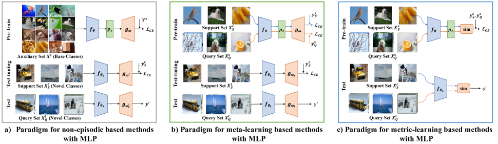
Fig. 2: The frameworks with MLP in accordance with three types of few-shot classification methods. Firstly, we pre-train a feature extractor $f$, an MLP projector $p$ and a classifier $g$. $sim$ denotes the classifier that computes similarity, e.g., the nearest-neighbor classifier. MLP projector is removed in the meta-testing phase for evaluating the performance of the pre-trained feature extractor $f$.

• We initiate the first known and comprehensive effort to study MLP in CDFSC, and further introduce three distinct frameworks in accordance with three types of few-shot classification methods to verify the effectiveness of MLP.

• We empirically demonstrate that MLP helps existing few-shot classification algorithms significantly improve cross-domain generalization performance on 12 datasets and even compare favorably against state-of-the-art CDFSC algorithms.

• Our analyses indicate that MLP helps obtain better discriminative ability and mitigate the distribution shift. Additionally, we find that batch normalization plays the most crucial role in improving transferability.

2 Related Work

2.1 Few-Shot Classification

Few-Shot Classification (FSC) methods can be divided into three types. First, meta-learning based methods [7, 8] adopt a learning-to-learn paradigm, allowing models to learn from training data and apply this prior learning to improve performance on new tasks or domains. Second, metric-learning based methods [9, 10] employ a learning-to-compare paradigm, allowing models to compare the similarity or the distance of the representations between support set data and query set data. Finally, non-episodic based methods [6, 11] abandon the learning-to-learn paradigm and adopt the pre-training paradigm from transfer learning. In this work, we introduce three distinct frameworks in accordance with these three types of FSC methods by incorporating MLP in cross-domain few-shot setting.

2.2 Cross-Domain Few-Shot Classification

One line of CDFSC methods learns various features via data augmentation, such as adversarial task augmentation [12] which learns worst-case tasks, and random crop augmentation [13] which is used for self-supervision learning. Another family of CDFSC methods aims to align features by using affine transforms [14] and hyperbolic tangent transformation [15] to minimize the distribution discrepancy between training and test datasets. However, these methods often result in complex optimization procedures and expensive computational complexity. In this study, we aim to shed new light on improving transferability with MLP, which only introduces a little computational complexity while ensuring simplicity and effectiveness in handling distribution-shift few-shot learning data.

3 Method

Type	Method	ChestX	CropD	DeepW	DTD	Euro	Flower	ISIC	Kaokore	Omni	Resisc	Sketch	SVHN	Average
Non-episodic	BL [11]	26.98	65.44	55.27	59.58	83.81	77.59	42.69	37.24	96.24	71.34	72.60	77.49	63.86
	BL+MLP	28.62	70.48	57.54	61.96	84.26	81.49	42.55	40.06	98.12	75.62	75.15	84.19	66.67 +2.81
	BL++ [11]	25.49	48.22	50.86	51.76	75.79	66.15	40.73	32.64	87.87	63.16	63.72	64.01	55.87
	BL+++MLP	28.09	65.62	57.65	64.33	85.83	81.47	44.32	38.14	97.47	74.76	75.85	82.30	66.32 +10.45
	RFS [6]	27.68	58.38	51.02	62.31	76.33	75.62	41.05	35.70	90.55	73.82	73.05	63.22	60.73
	RFS+MLP	29.09	66.87	56.42	67.78	83.14	86.24	46.02	42.31	97.95	80.04	77.64	81.27	67.90 +7.17
Meta-learning	ANIL [8]	24.41	48.69	46.93	46.55	63.96	61.27	37.57	31.50	84.53	58.92	61.90	58.29	52.04
	ANIL+MLP	25.02	58.10	49.35	53.30	75.73	66.45	39.19	32.61	83.02	64.62	61.70	51.97	55.09 +3.05
	MTL [16]	24.15	33.27	43.14	49.43	54.27	58.18	35.56	31.36	72.77	57.93	60.53	52.72	47.78
	MTL+MLP	25.19	51.23	46.06	49.41	65.19	51.34	34.74	31.59	78.84	53.97	51.62	52.01	49.27 +1.49
Metric-learning	PN [10]	26.38	55.59	47.50	50.55	70.96	63.56	32.95	33.58	92.68	58.70	54.53	64.38	54.28
	PN+MLP	27.07	60.76	47.83	50.49	73.22	62.63	33.76	32.00	87.06	59.02	51.85	66.69	54.37 +0.09
	DN4 [17]	27.34	53.62	50.94	58.67	76.52	75.01	42.68	37.67	97.43	70.30	72.81	84.76	62.31
	DN4+MLP	28.38	67.48	56.40	62.15	82.61	80.78	39.41	40.15	98.17	75.78	75.77	88.18	66.27 +3.96
	CAN [18]	27.46	52.82	53.14	56.85	73.77	71.40	42.32	36.55	83.03	69.96	66.03	58.32	57.64
	CAN+MLP	28.57	67.63	58.93	64.31	83.66	79.81	42.73	38.00	97.08	75.68	73.64	71.54	65.13 +7.49

Table 1: Comparisons with the vanilla baselines in 5-way 5-shot setting on 12 datasets with ResNet12 as the backbone. Bold denotes the best average scores, and underline denotes our method outperforms the vanilla methods by a large margin of more than 5.00%.

As shown in Figure 2, we adapt MLP to three types of FSC methods, i.e., non-episodic, meta-learning and metric-learning based methods. Specifically, our method mainly consists of a feature extractor $f(\cdot)$, an MLP projector $p(\cdot)$, and a classifier $g(\cdot)$ or similarity function $sim(\cdot)$. The MLP projector consists of two fully connected layers $fc$, a batch normalization layer $BN$, and a ReLU layer $ReLU$, which can be denoted as:

$$p(\cdot)=fc_{2}(ReLU(BN(fc_{1}(\cdot))).$$ (1)

In detail, the dimensions of the fully connected layers are set to be the same as the dimensions of the output of the feature extractor. We introduce three paradigms as follows.

Paradigm for non-episodic based methods with MLP. During the training phase, we divide the auxiliary set $X^{s}$ from the source dataset $D_{s}$ into batches of samples $T^{s}=\{X^{s}_{i}\}_{i=1}$, and denote the corresponding global labels as $Y^{s}_{i}$. We use the cross-entropy loss function to train our model:

$$\theta_{s},\varepsilon_{s},\omega_{s}=\underset{\theta,\varepsilon,\omega}{\arg\min}\sum_{i=1}^{N}\mathcal{L}^{\mathrm{CE}}\left(g_{\omega}\left(p_{\varepsilon}\left(f_{\theta}\left(X^{s}_{i}\right)\right)\right),Y^{s}_{i}\right),$$ (2)

where $\theta,\varepsilon,\omega$ are the parameters of the feature extractor, the MLP and the classifier, respectively. During the test-tuning phase, we divide the target dataset into amounts of tasks, and each task can be divided into the a support set $X^{t}_{S}$ and a query set $X^{t}_{Q}$. The support set data are used to fine-tune a new classifier $g_{\omega^{\prime}}$. The optimization function of one loop can be formulated as:

Method	RFS	RFS+MLP	RFS	RFS+MLP
Dataset	ChestX		CropD
$D_{1}$ ($\downarrow$)	6.85	6.78	6.37	5.83
$V$ ($\downarrow$)	2.73	2.69	2.64	2.61
$r$ ($\downarrow$)	1.21	1.20	0.85	0.80
Dataset	Euro		ISIC
$D_{1}$ ($\downarrow$)	3.83	3.57	6.09	5.66
$V$ ($\downarrow$)	1.73	1.51	2.35	2.05
$r$ ($\downarrow$)	0.49	0.43	1.04	0.92

Table 2: Quantitative analysis of features learned by RFS and RFS+MLP on CD-FSL benchmark. $D_{1}$ is the averaged $L_{2}$ inner-class distance, and $V$ is the inner-class variance, and $r$ is the ratio between the average of inner-class distance and the inter-class distance. Bold denotes the best scores.

$$\omega^{\prime}_{t} =\underset{\omega}{\arg\min}\mathcal{L}^{\mathrm{CE}}\left(g_{{\omega^{\prime}}}\left(f_{\theta_{s}}\left(X^{t}_{S}\right)\right),Y^{t}_{S}\right).$$ (3)

After the model is adapted to the support set, the query set data is used to evaluate the model performance.

Paradigm for Meta-learning Based Methods with MLP. During the training phase, we divide the auxiliary set $X^{s}$ from the source dataset $D_{s}$ into amounts of tasks $T^{s}=\{X^{s}_{i}\}_{i=1}$, which can be split into support set $T^{s}_{Si}=\{{X^{s}_{Si}}\}_{i=1}$ and query set $T^{s}_{Qi}=\{{X^{s}_{Qi}}\}_{i=1}$. The corresponding local labels are denoted as $y^{s}_{Si}$ and $y^{s}_{Qi}$. The support set data are used to train our model, thus the optimization function of one inner loop can be formulated as:

$$\theta^{\prime}_{s},\varepsilon^{\prime}_{s},\omega^{\prime}_{s}=\underset{\theta,\varepsilon,\omega}{\arg\min}\mathcal{L}^{\mathrm{CE}}\left(g_{\omega}\left(p_{\varepsilon}\left(f_{\theta}\left(X^{s}_{Si}\right)\right)\right),y^{s}_{Si}\right).$$ (4)

The query set data are used to truly update the model, and the optimization function of the outer loop can be formulated as:

$$\theta_{s},\varepsilon_{s},\omega_{s}=\underset{\theta,\varepsilon,\omega}{\arg\min}\mathcal{L}^{\mathrm{CE}}\left(g_{\omega^{\prime}_{s}}\left(p_{\varepsilon^{\prime}_{s}}\left(f_{\theta^{\prime}_{s}}\left(X^{s}_{Qi}\right)\right)\right),y^{s}_{Qi}\right).$$ (5)

During the test-tuning and test phase, it also adopts the paradigm of tuning on the support set of the target dataset (like Equation 4) and finally testing on the query set of the target dataset.

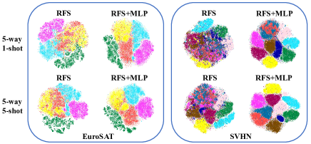
Fig. 3: The t-SNE visualization of RFS and RFS+MLP on EuroSAT and SVHN datasets with ResNet12 backbone in 5-way 1-shot and 5-way 5-shot settings. Different colors denote different classes.

Paradigm for Metric-learning Based Methods with MLP. Taking ProtoNet [10] as an example, it leverages the support set to calculate the mean centroid of the features. We denote $X^{s}_{i,j}$ as j-th sample in i-th class from the support set, thus the prototype can be defined as $c^{s}_{i}=1/K\sum^{K}_{j=1}f_{\theta_{s}}(X^{s}_{i,j})$, where $K$ denotes the number of images per class. Therefore, the probability of a query image $X^{s}_{Q}$ of the source dataset belonging to the i-th class can be formulated as:

$$P(y^{s}_{Q}=i\mid X^{s}_{Q})=\frac{\exp\left(-sim\left(p_{\varepsilon}(f_{\theta}(X^{s}_{Q})),c_{i}\right)\right)}{\sum^{C}_{j}\exp\left(-sim\left(p_{\varepsilon}(f_{\theta}(X^{s}_{Q})),c_{j}\right)\right)},$$ (6)

where $sim$ is a distance function or similarity function. Specifically, during the training phase, the cross-entropy loss is employed to train the model. Also, during the test phase, the nearest-neighbor classifier (like Equation 6) can be conveniently used for prediction.

4 Experiments

4.1 Experimental Setting

Datasets. During the training phase, we train our model on miniImageNet dataset [9] from scratch, which consists of 50,000 training images and 10,000 testing images, evenly distributed across 100 classes. We use the train set of miniImageNet for training. During the test-tuning phase, we evaluate the generalization performance on 12 datasets, i.e., CD-FSL benchmark [19] (including ChestX-ray (ChestX) [20], CropDisease (CropD) [21], EuroSAT (Euro) [22], ISIC [23]), DeepWeeds (DeepW) [24], DTD [25], Flower102 (Flower) [26], Kaokore [27], Omniglot (Omni) [28], Resisc45 (Resisc) [29], Sketch [30] and SVHN [31], following the setup in [5].

Method	ChestX	CropD	Euro	ISIC	Average
MatchingNet [9]	22.40	66.39	64.45	36.74	47.50
PN [10]	23.41	75.17	68.95	37.04	51.14
PN+FWT [14]	23.77	85.82	67.34	38.87	53.95
RN [32]	22.96	68.99	61.31	39.41	48.17
RN+FWT [14]	23.95	75.78	69.13	38.68	51.89
RN+ATA [12]	24.43	78.20	71.02	40.38	53.51
TPN+ATA [12]	23.60	88.15	79.47	45.83	59.26
RDC [15]	25.91	88.90	77.15	41.28	58.31
LDP-net [13]	26.67	89.40	82.01	48.06	61.54
BL+MLP (Ours)	25.70	89.36	79.62	44.61	59.82
RFS+MLP (Ours)	26.00	89.68	78.13	46.33	60.04

Table 3: Comparisons with SOTA methods in 5-way 5-shot setting on CD-FSL with ResNet10 as the backbone. Bold denotes the best scores and underline denotes the second-best scores.

Baselines. We choose 10 baselines for evaluating the effectiveness of our method. For non-episodic based methods, we adopt Baseline (BL) [11], Baseline++ (BL++) [11] and RFS [6]. For meta-learning based methods, we adopt MAML [7], ANIL [8], BOIL [33] and MTL [16]. For metric-learning based methods, we adopt ProtoNet (PN) [10], DN4 [17] and CAN [18]. Furthermore, we compare our method with state-of-the-art (SOTA) methods, including MatchingNet [9], ProtoNet (PN) [10], RelationNet (RN) [32], FWT [14], ATA [12], RDC [15] and LDP-net [13].

Experimental Setup. We mainly use three backbones as the feature extractor to evaluate the effectiveness of MLP, i.e., Conv64F, ResNet12 and ResNet18. For the training phase, we train all the models for 100 epochs on miniImageNet with SGD optimizer. The learning rate is set to vary within the range of 0.001 to 0.1 across different methods. The momentum rate is 0.9 and the weight decay is 5e-4. The learning rate decay strategy is based on cosine decay. For non-episodic based methods, we set the batch size to 128. For the other two types of methods, we set 2000 episodes in one epoch. For evaluation, we use the same 600 randomly sampled few-shot episodes for consistency, and report the averaged top-1 accuracy.

4.2 Analysis Experiments

The reasons behind the improved transferability achieved by MLP are: 1) MLP can mitigate the distribution shift between the pre-training and evaluation datasets. As shown in Figure 1, MLP significantly reduces the KL divergence between the pre-training and evaluation datasets, resulting in higher accuracy. 2) MLP can help the model obtain better discriminative ability in terms of cluster compactness. As shown in Table 2, the quantitative experiment demonstrates that when employing MLP, there are improvements in lower intra-class distance, intra-class variance, and the ratio between the average intra-class distance and inter-class distance. This indicates that MLP can make the learned representations more discriminable. Qualitatively, in Figure 3, we can also observe that MLP can help the model obtain better discriminative ability.

4.3 Comparisons

Comparisons with vanilla FSC methods. Table 1 demonstrates that all methods with MLP outperform the vanilla methods. For instance, BL++, RFS and CAN with MLP outperform the vanilla methods by a large margin of 10.45%, 7.17% and 7.49% on 12 datasets for the averaged top-1 accuracy, respectively. For some methods, there can be a large improvement on some datasets, e.g., +14.05% for CAN on Omniglot and +18.05% for RFS on SVHN, indicating MLP can significantly enhance the generalization performance of existing FSC methods.

Example	Input FC	BN	ReLU	Output FC	Acc.
(a)					60.73
(b)	$\checkmark$				61.03 (+0.30)
(c)	$\checkmark$	$\checkmark$			67.66 (+6.93)
(d)	$\checkmark$		$\checkmark$		61.14 (+0.41)
(e)	$\checkmark$	$\checkmark$		$\checkmark$	67.14 (+6.41)
(f)	$\checkmark$		$\checkmark$	$\checkmark$	62.05 (+1.32)
(g)	$\checkmark$	$\checkmark$	$\checkmark$		67.61 (+6.88)
RFS+MLP	$\checkmark$	$\checkmark$	$\checkmark$	$\checkmark$	67.90 (+7.17)

Table 4: Ablation on different components of MLP. The average results of 12 datasets are reported. Improvements over the baseline of RFS w/o MLP are marked in green.

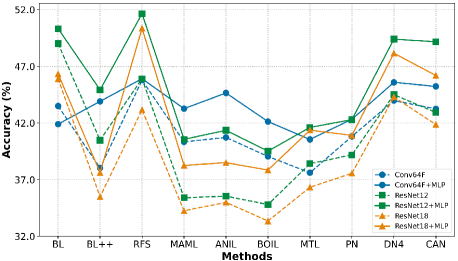
Fig. 4: Investigations on various backbones in 5-way 1-shot setting on 12 datasets. Different colors denote different backbones.

Comparisons with SOTA CDFSC methods. As shown in Table 3, in 5-way 5-shot setting, the averaged result of our method can reach around 60%, which is superior to and competitive to most of the state-of-the-art CDFSC algorithms. Our method incorporates an MLP to learn a more transferable feature extractor. This brings about only a marginal increase in computational complexity, further demonstrating the simplicity and effectiveness of our method.

4.4 Ablation Study

Effectiveness of different components in MLP. As shown in Table 4, we observe that integrating all components of MLP achieves the best accuracy among all variants. Furthermore, we find that Batch Normalization layer plays the most important role in enhancing the transferability of the model, whereas the linear layer and ReLU activation function are comparatively less influential.

Effectiveness of different backbones. As shown in Figure 4, we observe that MLP is efficient across different backbones, particularly when employed with more sophisticated backbone architectures. For the Conv64F backbone, most methods with MLP outperform vanilla methods by 0$\sim$3%, and by 3$\sim$6% for the ResNet12 and the ResNet18 backbone on 12 datasets.

5 Conclusion

In this paper, we initiate the first empirical study on using MLP for cross-domain few-shot classification. To verify the effectiveness of MLP in the few-shot setting, we introduce three distinct frameworks incorporating MLP in accordance with three types of few-shot classification methods. Based on empirical results, we identify that the MLP helps the model obtain better discriminative ability and mitigate the distribution shift, which results in good transferability. Our findings are confirmed with extensive experiments on various few-shot classification algorithms and diverse backbone networks.

References

- [1] Ting Chen, Simon Kornblith, Mohammad Norouzi, and Geoffrey Hinton, “A simple framework for contrastive learning of visual representations,” in ICML, 2020.
- [2] Xinlei Chen, Haoqi Fan, Ross Girshick, and Kaiming He, “Improved baselines with momentum contrastive learning,” arXiv, 2020.
- [3] Ashraful Islam, Chun-Fu Richard Chen, Rameswar Panda, Leonid Karlinsky, Richard Radke, and Rogerio Feris, “A broad study on the transferability of visual representations with contrastive learning,” in ICCV, 2021.
- [4] Prannay Khosla, Piotr Teterwak, Chen Wang, Aaron Sarna, Yonglong Tian, Phillip Isola, Aaron Maschinot, Ce Liu, and Dilip Krishnan, “Supervised contrastive learning,” NeurIPS, 2020.
- [5] Yizhou Wang, Shixiang Tang, Feng Zhu, Lei Bai, Rui Zhao, Donglian Qi, and Wanli Ouyang, “Revisiting the transferability of supervised pretraining: an mlp perspective,” in CVPR, 2022.
- [6] Yonglong Tian, Yue Wang, Dilip Krishnan, Joshua B Tenenbaum, and Phillip Isola, “Rethinking few-shot image classification: a good embedding is all you need?,” in ECCV, 2020.
- [7] Chelsea Finn, Pieter Abbeel, and Sergey Levine, “Model-agnostic meta-learning for fast adaptation of deep networks,” in ICML, 2017.
- [8] Aniruddh Raghu, Maithra Raghu, Samy Bengio, and Oriol Vinyals, “Rapid learning or feature reuse? towards understanding the effectiveness of maml,” ICLR, 2020.
- [9] Oriol Vinyals, Charles Blundell, Timothy Lillicrap, Daan Wierstra, et al., “Matching networks for one shot learning,” NeurIPS, 2016.
- [10] Jake Snell, Kevin Swersky, and Richard Zemel, “Prototypical networks for few-shot learning,” NeurIPS, 2017.
- [11] Wei-Yu Chen, Yen-Cheng Liu, Zsolt Kira, Yu-Chiang Frank Wang, and Jia-Bin Huang, “A closer look at few-shot classification,” in ICLR, 2019.
- [12] Haoqing Wang and Zhi-Hong Deng, “Cross-domain few-shot classification via adversarial task augmentation,” IJCAI, 2021.
- [13] Fei Zhou, Peng Wang, Lei Zhang, Wei Wei, and Yanning Zhang, “Revisiting prototypical network for cross domain few-shot learning,” in CVPR, 2023.
- [14] Hung-Yu Tseng, Hsin-Ying Lee, Jia-Bin Huang, and Ming-Hsuan Yang, “Cross-domain few-shot classification via learned feature-wise transformation,” arXiv, 2020.
- [15] Pan Li, Shaogang Gong, Chengjie Wang, and Yanwei Fu, “Ranking distance calibration for cross-domain few-shot learning,” in CVPR, 2022.
- [16] Qianru Sun, Yaoyao Liu, Tat-Seng Chua, and Bernt Schiele, “Meta-transfer learning for few-shot learning,” in CVPR, 2019.
- [17] Wenbin Li, Lei Wang, Jinglin Xu, Jing Huo, Yang Gao, and Jiebo Luo, “Revisiting local descriptor based image-to-class measure for few-shot learning,” in CVPR, 2019.
- [18] Ruibing Hou, Hong Chang, Bingpeng Ma, Shiguang Shan, and Xilin Chen, “Cross attention network for few-shot classification,” NeurIPS, 2019.
- [19] Yunhui Guo, Noel C Codella, Leonid Karlinsky, James V Codella, John R Smith, Kate Saenko, Tajana Rosing, and Rogerio Feris, “A broader study of cross-domain few-shot learning,” in ECCV, 2020.
- [20] Xiaosong Wang, Yifan Peng, Le Lu, Zhiyong Lu, Mohammadhadi Bagheri, and Ronald M Summers, “Chestx-ray8: Hospital-scale chest x-ray database and benchmarks on weakly-supervised classification and localization of common thorax diseases,” in CVPR, 2017.
- [21] Sharada P Mohanty, David P Hughes, and Marcel Salathé, “Using deep learning for image-based plant disease detection,” Front. Plant Sci., 2016.
- [22] Patrick Helber, Benjamin Bischke, Andreas Dengel, and Damian Borth, “Eurosat: A novel dataset and deep learning benchmark for land use and land cover classification,” IEEE J-STARS, 2019.
- [23] Noel Codella, Veronica Rotemberg, Philipp Tschandl, M Emre Celebi, Stephen Dusza, David Gutman, Brian Helba, Aadi Kalloo, Konstantinos Liopyris, Michael Marchetti, et al., “Skin lesion analysis toward melanoma detection 2018: A challenge hosted by the international skin imaging collaboration (isic),” arXiv, 2019.
- [24] Alex Olsen, Dmitry A Konovalov, Bronson Philippa, Peter Ridd, Jake C Wood, Jamie Johns, Wesley Banks, Benjamin Girgenti, Owen Kenny, James Whinney, et al., “Deepweeds: A multiclass weed species image dataset for deep learning,” Scientific reports, 2019.
- [25] Mircea Cimpoi, Subhransu Maji, Iasonas Kokkinos, Sammy Mohamed, and Andrea Vedaldi, “Describing textures in the wild,” in CVPR, 2014.
- [26] Maria-Elena Nilsback and Andrew Zisserman, “Automated flower classification over a large number of classes,” in CVGIP, 2008.
- [27] Yingtao Tian, Chikahiko Suzuki, Tarin Clanuwat, Mikel Bober-Irizar, Alex Lamb, and Asanobu Kitamoto, “Kaokore: A pre-modern japanese art facial expression dataset,” arXiv, 2020.
- [28] Brenden M Lake, Ruslan Salakhutdinov, and Joshua B Tenenbaum, “Human-level concept learning through probabilistic program induction,” Science, 2015.
- [29] Gong Cheng, Junwei Han, and Xiaoqiang Lu, “Remote sensing image scene classification: Benchmark and state of the art,” Proceedings of the IEEE, 2017.
- [30] Haohan Wang, Songwei Ge, Zachary Lipton, and Eric P Xing, “Learning robust global representations by penalizing local predictive power,” in NeurIPS, 2019.
- [31] Yuval Netzer, Tao Wang, Adam Coates, Alessandro Bissacco, Bo Wu, and Andrew Y Ng, “Reading digits in natural images with unsupervised feature learning,” NeurIPS Workshop, 2011.
- [32] Flood Sung, Yongxin Yang, Li Zhang, Tao Xiang, Philip HS Torr, and Timothy M Hospedales, “Learning to compare: Relation network for few-shot learning,” in CVPR, 2018.
- [33] Jaehoon Oh, Hyungjun Yoo, ChangHwan Kim, and Se-Young Yun, “Boil: Towards representation change for few-shot learning,” ICLR, 2021.