Enhancing Data Lakes with GraphAr: Efficient Graph Data Management with a Specialized Storage Scheme

Abstract

Data lakes, increasingly adopted for their ability to store and analyze diverse types of data, commonly use columnar storage formats like Parquet and ORC for handling relational tables. However, these traditional setups fall short when it comes to efficiently managing graph data, particularly those conforming to the Labeled Property Graph (LPG) model. To address this gap, this paper introduces GraphAr, a specialized storage scheme designed to enhance existing data lakes for efficient graph data management. Leveraging the strengths of Parquet, GraphAr captures LPG semantics precisely and facilitates graph-specific operations such as neighbor retrieval and label filtering. Through innovative data organization, encoding, and decoding techniques, GraphAr dramatically improves performance. Our evaluations reveal that GraphAr outperforms conventional Parquet and Acero-based methods, achieving an average speedup of $3283\times$ for neighbor retrieval, $6.0\times$ for label filtering, and $29.5\times$ for end-to-end workloads. These findings highlight GraphAr’s potential to extend the utility of data lakes by enabling efficient graph data management.

1 Introduction

Data lakes have quickly become an essential infrastructure for organizations looking to store and analyze diverse datasets in their raw formats [64, 22, 28, 48, 47, 41, 53]. As centralized repositories, they offer unparalleled flexibility in accommodating a wide array of data types, from structured relational tables to unstructured logs and text files. Crucially, they serve as a cost-effective solution for archiving data at scale while still allowing for queries on archived or rarely accessed data. This dual utility makes them invaluable for both real-time analytics and long-term data management. Columnar storage formats like Parquet [5] and ORC [4] have become standard for storing tabular data in data lakes due to their robust compression and efficient query capabilities.

In sync with these trends, graph data has become increasingly importance, especially for modeling complex relationships. Leading graph databases like Neo4j [13], TigerGraph [31], and JanusGraph [10] leverage the Labeled Property Graph (LPG) model [20, 23, 21] for this purpose. The recent ISO SQL:2023 standard includes a SQL/PGQ extension that not only facilitates querying property graphs but also enables the creation of property graph views from relational tables [19]. This groundbreaking inclusion highlights the growing convergence of relational and graph data models and emphasizes the need to integrate LPGs into data lakes. Consequently, LPGs are making their way into data lakes for multiple uses, from backups and archival storage for existing graph databases to natural extensions of transactional, log, and tabular data.

Managing and analyzing LPGs in data lakes offers several significant benefits. Graph-specific queries are often more naturally articulated in languages like Cypher [35], Gremlin [55], GQL [34], or SQL/PGQ, providing an intuitive framework for conducting comprehensive analysis of entity relationships, facilitating the discovery of valuable insights. Data lakes also provide computational flexibility for running complex graph algorithms, enabling the exploration of intricate patterns. Additionally, they offer cost-effective storage solutions, allowing organizations to utilize more affordable and colder storage options without sacrificing query performance. Most notably, data lakes enable seamless querying across both graph and relational data, ushering in a holistic approach to data analytics.

Figure 1: A graph-related query within the data lake.

As shown in Figure 1, the example workload illustrates a scenario of immense relevance to public health researchers. The query aims to count the number of families—comprising a father, mother, and child—each labeled as Asian and Enrollee (indicating their participation in a health study), and diagnosed with hypertension since 2020. Such queries hold significant utility for public health studies as they allow for the analysis of correlations between familial relationships, racial groups, and specific health conditions like hypertension among study participants. Understanding these relationships can be critical for targeted health interventions and for identifying possible social or genetic factors contributing to disease prevalence. Within the context of this research query, data lakes offer an economical and scalable solution for storing diverse, multi-source, and often historical health-related data. More importantly, the intricate relationships and multiple attributes required by this research are more naturally and efficiently captured through property graph queries than through traditional SQL. However, integrating LPGs into data lakes introduces unique challenges:

Firstly, there is no standardized way to encapsulate an LPG within the existing data lake architecture. While columnar formats like Parquet and ORC excel at storing individual tables, they fall short in representing the complex relationships and semantics across these tables, which are inherent to LPGs.

Secondly, executing graph-specific operations, particularly neighbor retrieval and label filtering, can be highly inefficient in this setup. For example, neighbor retrieval might require multiple joins, significantly impacting performance. Label filtering, another essential operation, also introduces inefficiency due to the lack of native support in columnar formats.

GraphAr. To address these challenges, we introduce GraphAr, an efficient storage scheme for graph data in data lakes. GraphAr is designed to enhance the efficiency of data lakes while utilizing the capabilities of existing formats, with a specific focus on Parquet in this paper. GraphAr ensures seamless integration with existing tools and introduces innovative additions specifically tailored to handle LPGs.

Firstly, Parquet provides flexible and efficient support for various datatypes, including atomic types (e.g., bools and integers), and nested and/or repeated structures (e.g., arrays and maps). Using Parquet as fundamental building block, GraphAr further introduces standardized YAML files to represent the schema metadata for LPGs. This combination of data organization and metadata management enables the complete expression of LPG semantics, while ensuring compatibility with both data lakes and graph-related systems.

Secondly, GraphAr incorporates specialized optimization techniques to improve the performance of two critical graph operations: neighbor retrieval and label filtering, which are not inherently optimized in existing formats. GraphAr facilitates neighbor retrieval by organizing edges as sorted tables in Parquet to enable an efficient CSR/CSC-like representation, and leveraging Parquet’s delta encoding to reduce overhead in data storage and loading. GraphAr also introduces a novel decoding algorithm that utilizes BMI and SIMD instructions, along with a unique structure named PAC (page-aligned collections), to further accelerate the neighbor retrieval process. In addressing another critical aspect of LPGs, GraphAr adapts the run-length encoding (RLE) technique from Parquet and introduces a unique merge-based decoding algorithm. This tailored approach significantly improves label filtering performance, whether it involves simple or complex conditions.

Our key contributions can be summarized as follows:

• Elucidation of challenges and limitations in existing tabular formats for managing LPGs in data lakes (Section 2).

• A strategic choice of Parquet compatibility, a standardized YAML to fully express LPG semantics, and detailed specification for organizing LPGs in Parquet (Section 3).

• Development of specialized optimization techniques for enhancing performance in neighbor retrieval and label filtering operations (Sections 4 and 5).

• Comprehensive performance evaluation of GraphAr compared to Parquet and Acero-based implementations, highlighting substantial speed gains: on average $3283\times$ for neighbor retrieval, $6.0\times$ for label filtering, and $29.5\times$ for end-to-end workloads (Section 6).

2 Background and Key Challenges

In this section, we discuss the limitations of using tabular formats like Parquet and ORC in data lakes for LPGs, a common graph data model. We explore how these formats inadequately support LPG representation and efficient graph queries, laying the groundwork for the challenges that GraphAr tackles, outlined at the section’s end.

2.1 Tabular Formats in Data Lakes

Tabular data is key to data lakes, aiding efficient organization, analysis, and data extraction from large sets. Columnar formats like Parquet [5] and ORC [4] are popular due to their robust features. Unlike row-based formats such as CSV, they allow faster queries by enabling selective column reading, avoiding unnecessary data. Additionally, they offer diverse and efficient compression and encoding strategies, such as delta encoding to compress the variance between consecutive values, and run-length encoding to compress repetitive values. These techniques not only reduce storage needs but also enhance processing speeds. Another advantage of Parquet and ORC is predicate pushdown, which enhances query performance by moving filters closer to the storage layer, thereby reducing subsequent data reads.

The combination of selective column reading, efficient compression, and predicate pushdown positions Parquet and ORC as the go-to choices for managing tabular data in data lakes. Previous studies have demonstrated the importance of leveraging their capabilities for optimizing relational data management [33, 40, 22]. Recent research [45, 60, 61, 62, 63, 6] has also explored enhancements to tabular formats, utilizing CPU instruction sets like BMI and SIMD. In this paper, we will focus on Parquet, but the techniques discussed can be seamlessly adapted to other columnar formats such as ORC.

Figure 2: The internal structure of a Parquet file for a logical table with $C$ columns and $R$ row groups.

Parquet. Figure 2 illustrates the internal structure of a Parquet file. Structurally, a Parquet file represents a table, organized into row groups for logical segmentation. Within a row group, the data of a column is stored in a column chunk, which is guaranteed to be contiguous in the file. Column chunks are further divided into pages, which are the indivisible units for data compression and encoding. These pages, which can vary in type, are interleaved in a column chunk.

Parquet files contain three layers of metadata: file metadata, column metadata, and page header metadata. The file metadata directs to the starting points of each column’s metadata. Inside the column chunks and pages, the respective column and page header metadata are stored, offering a detailed description of the data. This includes data types, encoding, and compression schemes, facilitating efficient and selective access to data pages within columns.

2.2 Labeled Property Graphs

Labeled Property Graphs (LPGs) [20, 23, 21] excel at representing complex relationships and semantics in a natural manner. Their flexible schema allows for accommodating the diverse and evolving nature of big data within repositories, making them integral to data lakes. LPG serves as the canonical data model in many graph systems [13, 36, 31] and graph query languages [59, 7, 35, 55, 34, 30], enabling queries and analytics to uncover valuable insights and patterns. Formally, an LPG is defined as $G=(V,E,T_{V},T_{E},P,L)$, where $V$ is a set of vertices, $E$ a set of edges, $T_{V}$ and $T_{E}$ the types of vertices and edges respectively, $P$ the properties, and $L$ the labels.

For each vertex $v\in V$ and edge $e\in E$, they are associated with a type $t_{v}\in T_{V}$ and $t_{e}\in T_{E}$ respectively, and can have optional properties. A property $p\in P$ is specific to a vertex or an edge type, with a unique identifier within its type and a pre-defined datatype for its values. This implies that vertices or edges of the same type share the same set of properties.

Furthermore, each label $l\in L$ has a unique identifier, usually a string. Each vertex type $t_{v}$ is linked with a set of candidate labels $L(t_{v})\subseteq L$, allowing each vertex of this type to be assigned zero or more labels. Labels hold significant importance in LPGs as they represent classifications and characteristics of entities, whereas properties serve as attributes to store additional information. Although edge types could technically also be labeled, in this paper, we focus solely on vertex labels, aligning with common graph query practice .

While Parquet is highly effective for storing individual vertex and edge types $T_{V}$ and $T_{E}$ along with their associated properties due to the columnar structure and data compression capabilities, it falls short in capturing the interconnected schema essential for linking vertices with edges, e.g., to express the relationships across the three tables of Figure 3, which represent two vertex types and one edge type. This limitation is crucial for efficient graph traversal and pattern matching. Moreover, Parquet lacks native support for the multi-labeling capability of LPGs, resulting in a loss of complex semantics and relationships inherent to LPGs.

Figure 3: An example of querying LPGs on tabular formats.

2.3 Querying Labeled Property Graphs

The core feature shared among existing graph query languages is the facility for pattern matching [30, 7]. This capability allows for in-depth analysis of the relationships between entities, uncovering valuable insights and patterns that may not be readily apparent in other data models. A graph pattern is defined as vertices and their connections through edges, filtered based on labels and property values [34]. Figure 3 illustrates the example workload mentioned in Figure 1, expressed in Cypher. And the steps for matching (a:Asian:Enrollee)-[e1:Diagnosed]->(d) are highlighted in the figure.

When it comes to properties, a viable approach is to use native tabular data. This leverages the storage efficiency of existing formats, while optimizing property-related operations in graph queries. However, this approach struggles with two crucial aspects of pattern matching.

Firstly, tabular formats lack native support for representing graph topology, making it difficult to efficiently fetch the neighboring vertices and edges for a given vertex. A common workaround is to store edge endpoints as properties and use the join operations across multiple tables to retrieve neighbors, as shown in Figure 3. However, this approach is often inefficient due to the computational overhead of multiple joins.

Secondly, LPGs allow vertices to have multiple labels, offering a flexible and expressive way to describe entities. Label filtering is an essential feature in graph queries, to enable the selection of specific subsets of vertices, making it a core element in all graph query languages [34, 7, 55, 59]. Existing formats do not natively accommodate this flexibility and do not provide a foundation for label-based optimizations. Encoding labels as ordinary properties and performing filtering by string matching, as seen in the initial step of Figure 3, limits the expressive power of vertex representation and hampers efficient label handling, a feature unique to graph queries.

These query-side inefficiencies highlight the limitations of using tabular formats for graphs. The reliance on suboptimal workarounds, such as multiple joins for topology expansion and makeshift encoding schemes for label filtering, compromises query performance and complicates the query process. This paves the way for the challenges we seek to address.

2.4 Key Challenges Addressed by GraphAr

The development of GraphAr is motivated by the specific limitations of existing tabular formats for both representing LPGs and supporting efficient graph queries.

Challenge 1: Effective LPG representation. LPGs use type-based organization and specific label/property definitions to form a cohesive graph structure. This enables precise and targeted querying. Existing tabular formats fall short of capturing these intricate semantics, necessitating a specialized solution. This challenge is addressed in Section 3.

Challenge 2: Efficient neighbor retrieval. A cornerstone of graph queries is the operation known as neighbor retrieval. This is vital for quick access to adjacent vertices and edges, thus accelerating graph traversal. Existing tabular formats, however, do not natively or efficiently support this crucial operation. This issue is tackled in Section 4.

Challenge 3: Optimized label filtering. Label filtering is a primary filtering mechanism in graph queries, allowing for the early elimination of irrelevant data. Existing tabular formats do not natively support this operation, making it a ripe area for optimization. This is the focus of Section 5.

Each of these challenges represents a gap in the capabilities of current tabular formats for graph data. They serve as the focus areas for the technical contributions of GraphAr, with each corresponding to a dedicated section in this paper.

(a) Metadata.

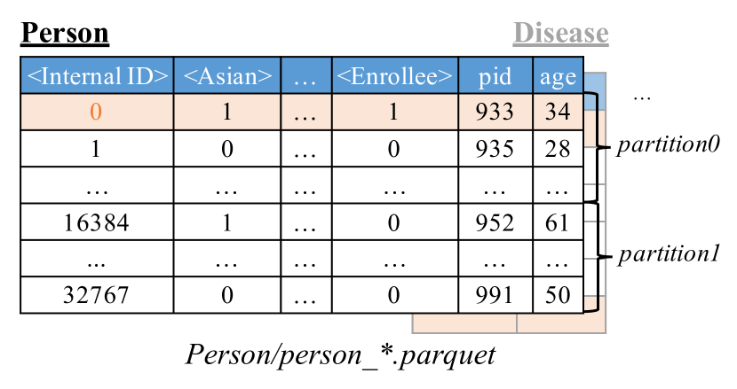
(b) Vertex table of Person (and Disease).

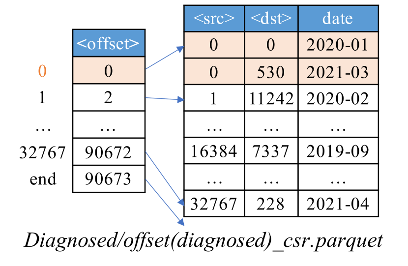
(c) Edge table of Person-Diagnosed-Disease.

Figure 4: The metadata and data layout for the example graph in GraphAr.

3 Representing LPGs in GraphAr

This section provides an overview of how GraphAr customizes the representation of LPGs in data lakes. It begins by outlining the goals and non-goals of GraphAr, providing clarity on the rationale behind its design. Next, it explains the strategies employed for data organization and layout, emphasizing the significance of schema metadata and the use of Parquet as the payload format. Lastly, the section describes how GraphAr seamlessly integrates into the data lake ecosystem.

3.1 Goals and Non-Goals

Goals. GraphAr’s primary goal is to provide an efficient storage scheme for LPGs in data lakes, specifically targeting the three main challenges outlined in Section 2.

GraphAr also seeks compatibility with both data lake and graph processing ecosystems for smooth integration with a variety of existing tools and systems.

Non-Goals. GraphAr does not intend to replace existing data lake formats like Parquet and ORC, but to maximize their benefits and offer additional features for LPGs.

In line with the established practices of data warehousing and lake house architectures, both Parquet/ORC and GraphAr adhere to data immutability norms, treating batch-generated data as immutable once created. Higher-level systems, such as graph databases, manage mutation and compaction (e.g., adding, deleting, or updating a vertex) through specialized, non-standardized file and in-memory versioning methods.

3.2 Data Organization and Layout

In GraphAr, vertices and edges are organized according to their types, which aligns with the principles of the LPG model. Parquet is utilized as the payload file format for storing the data in the physical storage, while YAML files are used to capture schema metadata.

Schema metadata. A YAML file, as illustrated in Figure 4(a), stores the metadata for a graph. This file specifies important attributes such as file path prefixes, and vertex/edge types. It serves as a nimble yet effective way to capture metadata that is not accommodated by Parquet, while Parquet files include specific details about properties and labels within their internal schemas. The YAML file can optionally include partition sizes, allowing for data to be segmented into multiple physical parquet files, thereby facilitating file-level parallelism.

Vertex table. As depicted in Figure 4(b), each row in the vertex table represents a unique vertex, identified by a 0-indexed internal ID, stored in the <Internal ID> column. Optionally, when partitioning is enabled, for the $i$-th partition, its internal IDs start at partition_size$\times i$, and within each partition, IDs are sorted in ascending order. Bubbles are allowed at the end of each partition, meaning the actual number of rows can be less than or equal to the partition size.

Property columns (pid and age) are named after their respective properties and hold the corresponding values with specified datatypes. In terms of labels, a set of candidate labels is defined for each vertex type. Then a vertex can have an arbitrary number of labels from the corresponding set. For example, the vertex type Person may have labels to represent ethnicity. For efficient storage and filtering of labels, GraphAr uses a binary representation to maintain each label in an individual column named with angle brackets, e.g., <Asian> and <Enrollee>. Additionally, advanced encoding/decoding techniques are applied, which will be discussed in Section 5.

Edge table. Edges are also organized and stored in Parquet files, similar to vertices. Figure 4(c) showcases the layout of the edge table for type Person-Diagnosed-Disease, where Person and Disease represent the source and destination vertex types, while Diagnosed signifies the classification of the relationships. Each edge is associated with the internal IDs of its source and destination vertices, stored in columns named <src> and <dst>. Edge properties, and optional partitioning, are handled in the same way as vertices.

Optimized access patterns for neighbor retrieval. The layout strategy in GraphAr leverages the columnar storage capabilities of Parquet to facilitate efficient graph traversal. Edges are sorted first by source vertex IDs and then by destination vertice IDs. This sorting strategy optimizes various access patterns. For row-wise access, the layout closely resembles the Coordinate List (COO) format, making it well-suited for edge-centric operations. On the other hand, an auxiliary index table, denoted as <offset>, is introduced to enable more efficient vertex-centric operations. The <offset> table aligns with the partitions in the vertex table, and when applied to the source vertices, facilitates retrieval patterns similar to Compressed Sparse Row (CSR). This separate index table accommodates scenarios where a vertex has multiple types of edges created separately from different data sources, a common occurrence in data lakes. Likewise, a similar approach can be applied to enable Compressed Sparse Column (CSC)-like access. GraphAr allows for efficient retrieval of neighbors in both outgoing and incoming directions, through two sorted tables for the same edge type. CSR, CSC, and COO are widely adopted for representing graphs, by emulating these formats, GraphAr ensures compatibility with existing graph systems.

These layout strategies are complemented by encoding and decoding optimizations, which are detailed in Section 4. Collectively, these strategies serve to enhance both the data management and query capabilities of GraphAr.

3.3 Incorporation with Data Lakes

The design of GraphAr makes it especially well-suited for integration with data lakes, largely due to its reliance on widely adopted standards like Parquet and YAML.

Data transformation and construction. The GraphAr format is essentially a specialized layout of Parquet files accompanied by a YAML metadata file. This enables the use of existing data processing frameworks like Apache Spark, Acero, and Hadoop, which can access various graph systems like Neo4j, TigerGraph and Nebula, or other types of database systems through their respective connectors. These frameworks can also ingest a multitude of data formats including logs, relational tables, JSON, and more. Such flexibility provides users with the ability to construct, transform, and store LPGs in data lakes from a wide array of data sources. To simplify the process of generating files in GraphAr, we have also provided a Spark library specifically designed for this purpose.

Downstream system integration. Since GraphAr is fundamentally based on Parquet and YAML, it is straightforward to use it as a data source for downstream systems. Many systems already have the capability to ingest Parquet files, making GraphAr a convenient and efficient data storage scheme.

Graph-specific optimizations. In addition to serving as a flexible storage format, GraphAr is also optimized for graph-specific operations. These optimizations, include advanced query pushdown techniques and other performance enhancements that are particularly useful for graph-specific tasks and queries within data lakes (see more from Sections 4 and 5).

4 Efficient Neighbor Retrieval

In this section, we address the critical challenge of efficient neighbor retrieval in graphs. We leverage Parquet’s data pages and introduce page-aligned collections (PAC) for streamlined neighbor identification. Additionally, we harness Parquet’s delta encoding as an efficiency-boosting technique. We then introduce a novel and optimized decoding strategy that leverages BMI and SIMD, using bitmaps as the data structure for collections in PAC. All of these techniques are integrated into GraphAr, resulting in highly efficient neighbor retrieval.

4.1 Workflow and Challenges

Parquet use data pages to match the data storage with the access granularity of the underlying storage layers, with a page represents the minimum unit of data that can be read from or written to the storage layer, as illustrated in Figure 2. And encoding and decoding are applied at the page level.

For LPG queries, a common operation is to retrieve specific property values of neighboring vertices, given a queried vertex, e.g., obtaining the name values of Disease vertices connected to a particular Person vertex. Assuming the CSR format utilized for storing edge table Person-Diagnosed-Disease, the typical workflow for this operation involves: 1) Using the <offset> index and <dst> column of the edge table to identify and fetch the first relevant page from the target vertex table (a page from the name column in the Disease table). This page contains at least one neighboring vertex pertinent to the query, and may also include other irrelevant vertices; 2) Selectively fetching the property values corresponding to the neighboring vertices within that page. This step is repeated iteratively for each subsequent page containing the targeted neighbors.

This workflow highlights the two primary tasks during neighbor retrieval. The first task is to identify which pages in the vertex table contain the neighboring vertices relevant to the query. The second task is to fetch the relevant property values within each of these pages efficiently. Before discussing our solutions, we formalize the neighbor retrieval operation:

Definition 1 (Page-aligned collections (PAC))

Given a column in vertex table that includes $m$ pages, the PAC $\mathcal{C}=[C_{0},\ldots,C_{m-1}]$ is a list of up to $m$ collections. Each $C_{i}$ stores a set of internal IDs in the corresponding page. Non-empty collections in $\mathcal{C}$ are retained, while empty ones are omitted.

Definition 2 (Neighbor Retrieval)

Given a vertex $v$, the operation of neighbor retrieval returns the PAC $\mathcal{C}$ representing the internal IDs of the neighboring vertices connected to $v$.

Intuition: Each collection $C$ in PAC returned by neighbor retrieval corresponds to a data page, addressing the first task. To save space and avoid unnecessary processing, empty collections are omitted from the PAC. This is based on the sparsity of real-world graphs, which often results in irrelevant pages. For the second task, the internal IDs within each collection enable the retrieval of only the relevant property values through a selection process. Afterwards, the remaining challenges involve efficiently generating PAC $\mathcal{C}$ and optimizing the data structure of each collection for quick value retrieval.

4.2 Delta Encoding

To compute the PAC $\mathcal{C}$, the encoded internal IDs of neighboring vertices need to be loaded, sourced from the edge table. In a data lake scenario, where data can be stored remotely, the loading process can be more time-consuming than processing due to I/O limitations. To address this issue, we investigate the use of delta encoding for data compression, consequently reducing the volume of data that needs to be loaded.

Delta encoding. Previous research, including Gemini [65] and Facebook-Graph [58], has demonstrated that real-world graphs often exhibit both sparsity and locality. This means that while a vertex’s neighbors might be spread across the entire graph, they are more likely to cluster within certain ID ranges. Such patterns arise from various factors, such as the inherent clustering in real-life graph data, where vertices within a cluster are more interconnected, and the methods used for graph data collection (e.g., crawlers or the organic/viral growth patterns of social networks like Facebook or TikTok). Systems [26, 65] have utilized such sparsity and locality to enable efficient partitioning or compression.

In GraphAr, such inherent locality, reinforced by our meticulous dual-key sorting of edges in the carefully designed layout, to enable incremental arrangement of internal IDs for a vertex’s neighbors, serves as the basis for delta encoding, which is highly effective for both the <src> and <dst> columns in the edge table. Delta encoding works by representing the gaps (deltas) between consecutive values instead of storing each value individually. The deltas, which often have small values, can be stored more compactly, requiring fewer bits.

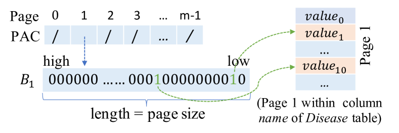
Figure 5: An example of PAC and the bitmap representation.

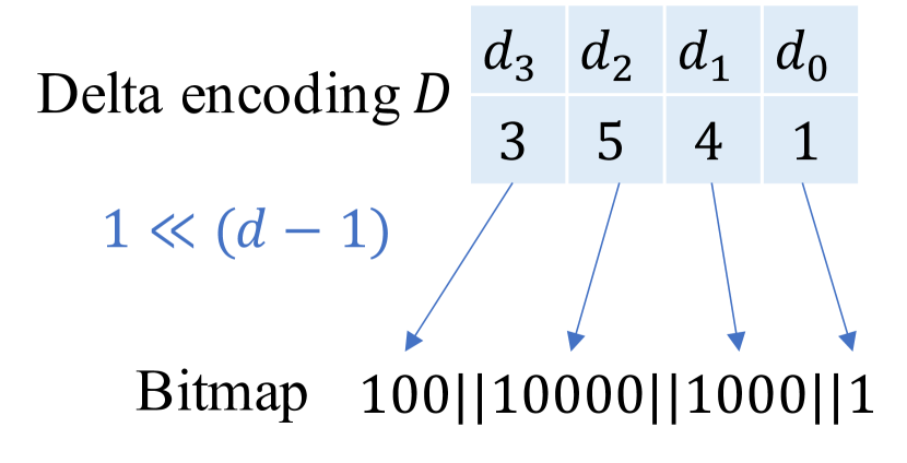
(a) Intuition.

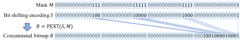
(b) Implementation.

Figure 6: An example of accelerating decoding via BMI.

Implementations. We utilize Parquet’s built-in support for delta encoding [43], which is implemented based on miniblocks. Each miniblock (with a size of $32$ values) is binary packed using its own bit width, which should be a power of 2 for data alignment purposes. This design allows us to adapt to changes in the data distribution, as the bit width of each miniblock is dynamically adjusted to minimize storage consumption. According to our evaluation across various real-world graphs, as detailed in Section 6.2, the delta encoding technique can reduce the expected loaded data volume (which can be measured by storage consumption) by $58.1\%$ to $81.0\%$ compared to without delta encoding. As a result, it brings an individual speedup of up to $3.6\times$ for neighbor retrieval.

4.3 BMI-based Decoding

Challenges. Whiles delta encoding effectively reduces loading costs, it introduces additional decoding computation. Existing works [45, 43, 61, 50, 51, 52] have explored the use of BMI (Bit Manipulation Instructions) and SIMD (Single Instruction, Multiple Data) to accelerate the data compression, decoding, scanning, or management. However, delta encoding involves data dependencies that make vectorization challenging. The decoding of the $(i+1)$-th neighbor depends on the prior decoding of the $i$-th neighbor.

Another unsolved issue is the choice of implementing collection $C$ in PAC. A pioneering solution proposed in [45] underscores the transformation of indices into a bitmap representation to enable selection pushdown in columnar storages. To adopt this approach to efficiently retrieve the properties of neighbors, which constitutes the second task of neighbor retrieval, we adopt a bitmap representation $B$ for each non-empty collection $C$ in PAC, where $B[i]=1$ indicates the existence of $i$-th element. Figure 5 illustrates a PAC and its bitmap representation, where only $C_{1}$ is non-empty, and $B_{1}$ is the bitmap representation of $C_{1}$. The bitmap representation can be used to facilitate the selection pushdown of vertex properties or labels, e.g., fetching the properties of name in the target vertex table Disease, for the neighbors of a person vertex.

Then, the critical challenge becomes how to efficiently generate the bitmap representation from the delta-encoded neighbor IDs. Existing techniques are not suitable for our context due to the data dependencies involved. However, by taking advantage of the sophisticated instruction sets offered by modern CPUs, we can exploit the functionalities of BMI together with SIMD operations to overcome this challenge, through an innovative decoding strategy.

Intuition. To ensure clarity, we initially consider a simplified scenario where each delta value is compressed to a 4-bit size. Conventionally, a two-step approach is used to decode the delta-encoded data, in which the current encoded value is added to the previously decoded ID to obtain the current ID, and then the bitmap is updated bit by bit based on the decoded IDs. However, our analysis reveals that this two-step process is redundant. By leveraging the bit-shifting encoding $1<<(d-1)$ for each delta value $d$, we can generate the bitmap by concatenating the bit-shifting encodings: $1<<(d_{n-1}-1)||\dots||1<<(d_{1}-1)||1<<(d_{0}-1)$, where $d_{0},d_{1},\dots,d_{n-1}$ represent $n$ delta values, and $||$ represents the concatenation operator. This principle is visually depicted in Figure 6(a).

Acceleration via BMI and SIMD. In practical implementation, the bit-shifting encoding is maintained using a fixed-length datatype, characterized by zero-padding on the left side. In our example, 16 bits are sufficient to accommodate the 4-bit delta values. The bit-shifting encodings of four values are stored in a 64-bit register, allowing for parallel generation and processing using SIMD instructions. Then, the focus shifts to the compaction of these encodings. Fortunately, the Parallel Bit Extract (PEXT) operation, a specialized CPU instruction in BMI, facilitates efficient aggregation of discrete bits from source positions into contiguous bits within the destination, governed by a selector mask, as illustrated in Figure 6(b).

The subsequent challenge is to generate the required mask, achieved by deriving the $i$-th mask $m_{i}$ from the $i$-th bit-shifting encoding $s_{i}$ using the equation $m_{i}=(s_{i}<<1)-1$. The beauty of this operation is its potential for parallel execution, facilitated by direct manipulation of the mask sequence residing within a 64-bit register. Specifically, $M$ can be acquired via the following steps: 1) a bitwise (in our example, 16 bits) shift of each $s_{i}$ to the left by 1 bit, parallelized through SIMD instructions like _mm_slli_epi16; and 2) a bitwise subtraction of 1 from the result of the previous step, which can be accelerated via instructions like _mm_sub_epi16. All these SIMD instructions utilized in our implementations are widely available in modern CPUs, included in SSE2 (which we use) and more recent sets such as AVX2 and AVX-512.

In general, vectorization demonstrates greater efficiency when the bit width is smaller, as it allows for more significant parallelism. Our extensive evaluations have confirmed that the BMI-based decoding approach outperforms the default decoding approach in Parquet when the bit width is within 4 bits, with performance improvements ranging from $3.2\%$ to $110\%$. Therefore, we utilize this BMI-based approach for miniblocks with a bit width of 1 to 4 bits, while resorting to the default delta decoding of Parquet for larger bit widths. The combination of data layout, delta encoding, and this adaptive decoding strategy results in an advanced topology management paradigm, enabling efficient neighbor retrieval.

5 Optimized Label Filtering

Labels serve as a representation of the classification or characteristics of vertices in a graph. Filtering vertices by labels is a fundamental syntax in graph query languages, as it allows querying specific subsets of vertices. However, existing approaches [8, 15] of fitting graphs into tabular data often treat labels as regular properties, encapsulating them within a string or list, as seen in Figure 3. These approaches overlook the inherent differences between labels and properties, leading to inefficiencies when performing label filtering, due to the need for decoding string representations and string matching.

Recognizing the widespread use of labels as filter conditions and their unique nature, we develop a specialized format for labels leveraging binary representation and run-length encoding (RLE), for handling simple conditions. To support complex conditions introduced by user-defined functions that involves multiple labels, we enhance our methodology with a novel merge-based decoding algorithm, further improving efficiency and adaptability.

5.1 Handling Simple Conditions

We start by considering the simple condition that focuses on the existence of a single label. In essence, the existence or absence of a label can be effectively represented using binary notation, where the value 1 indicates the existence of the label and 0 indicates its absence, as demonstrated in Figure 4(b). This binary representation offers two significant advantages: 1) it reduces the computational burden associated with decoding and matching as well as simplifies the filtering process as follows; 2) it enables efficient compression.

Definition 3 (Simple Condition Filtering)

Given a label $l$, and an existence/absence indicator $e$, the simple label filtering returns the PAC $\mathcal{C}$, where

$$\left\{\begin{aligned} v\in\mathcal{C},\text{ if }v.label[l]=e\\ v\notin\mathcal{C},\text{ if }v.label[l]\neq e\end{aligned}\right.$$ (1)

Encoding. To compress consecutive runs of 0s or 1s, we utilize the technique of run-length encoding (RLE), which represents them as a single number. This run-length format naturally transforms the binary representation of a label into an interval-based structure. We then adopt a list $P$ to define the positions of intervals. The $i$-th interval is represented by $[P[i],P[i+1])$, where $P[i]$ refers to the $i$-th element within $P$. Besides, it is required to record whether the vertices of the first interval $[P[0],P[1])$ contain the label or not, i.e., the first value. By leveraging this technique, the storage consumption of labels can be significantly reduced.

Decoding. Beyond efficient compression, the RLE approach seamlessly accommodates the decoding requirements for filter conditions. Specifically, to filter vertices with (or without) a specific label, we can simply select all odd intervals or all even intervals from the list $P$, based on the condition and the first value, instead of evaluating each vertex individually. It reduces the time complexity from $O(n)$ to $O(|P|)$, where $n$ represents the number of vertices and $|P|$ represents the size of the interval list $P$. In real-world graphs, $|P|\ll n$ is often observed, due to the sparsity of labels and natural clustering of vertices with similar labels.

5.2 Extending to Complex Conditions

Expanding beyond the realm of simple label existence, we encounter the intricacies of dealing with complex conditions involving multiple labels. Consider a scenario where we need to find vertices with specific label combinations, such as the GQL pattern MATCH (person:Asian&Enrollee) (or in Cypher, MATCH (person:Asian:Enrollee)), which retrieves vertices labeled as Asian and Enrollee. A more complex pattern can be MATCH (person:(Asian&!Enrollee)|Student), which retrieves vertices labeled as Asian but not Enrollee, or labeled as Student. To handle such scenarios, we employ user-defined functions (UDFs) to represent complex filter conditions. The UDF $f$ takes a vertex $v$ as input and returns a boolean value $f(v)$, indicating whether the vertex satisfies the condition or not. Formally, we define the complex condition filtering as follows.

Definition 4 (Complex Condition Filtering)

Given a UDF $f$, the filtering returns the PAC $\mathcal{C}$, where

$$\left\{\begin{aligned} v\in\mathcal{C},\text{ if }f(v)=\text{true}\\ v\notin\mathcal{C},\text{ if }f(v)=\text{false}\end{aligned}\right.$$ (2)

The intuitive approach would be to tackle each vertex independently, decoding the RLE format into the binary representation detailed earlier. However, a direct evaluation of the UDF for every vertex proves impractical, as it retains the same complexity as the most straightforward approach.

Intuition. Inspired by the concept of discretization, two key questions arise: 1) Can we solely evaluate the condition for one representative vertex within each interval? 2) How can we efficiently identify these intervals where the encompassed vertices share the same labels? The affirmative answer to the first question emerges through the following theorem:

Theorem 1

Consider $k$ interval lists $P_{0},P_{1},\dots,P_{k-1}$, where the vertices in $[P_{i}[j],P_{i}[j+1])$ share the same value for the $i$-th label. If an iterval $[s,e)$ is not broken by any position, i.e.,

$$\nexists i\in[0,k),j\in[0,|P_{i}|)\quad s<P_{i}[j]<e,$$ (3)

the vertices within the interval $[s,e)$ have the same labels, i.e.,

$$\forall u,v\in[s,e),l\in[0,k)\quad u.label[l]=v.label[l].$$ (4)

Consequently, it is sufficient to call the UDF for the vertex $s$ alone, as for any vertex $v$ in the interval $[s,e)$, $v$ and $s$ share the same labels thus $f(v)=f(s)$.

Figure 7: An example of merging intervals.

Merge-based algorithm. Partitioning an interval into multiple segments proves unnecessary and counterproductive as it would escalate complexity. Therefore, our focus narrows down to intervals formed by existing positions, which also addresses the second question. To obtain the exact intervals, we can sort the positions in all interval lists $P_{0},P_{1},\dots,P_{k-1}$. This sorting can be accelerated by leveraging the inherent order within the $k$ lists, allowing for seamless merging of $k$ sorted lists into one list $P$. Figure 7 demonstrates an example of interval determination for a complex condition containing two labels. Within the interval $[P[i],P[i+1])$, the vertices share identical labels, necessitating the UDF to be invoked solely for one representative vertex. Additionally, the presence of position $P[6]$ for both labels underscores the importance of merging to avoid redundant computations.

By employing innovative label treatment, interval-based encoding/decoding, and complex condition handling, GraphAr is able to achieve highly efficient label filtering.

6 Evaluation

In this section, we evaluate GraphAr on a range of real-world and synthetic graphs, through micro-benchmarks focusing on neighbor retrieval and label filtering, as well as end-to-end workloads. Our findings validate GraphAr as an efficient storage scheme for LPG storage and querying in data lakes.

Table 1: Statistics of the graphs in our evaluation.

Abbr.	Graph	$\mathbf{|V|}$	$\mathbf{|E|}$
AR	arabic-2005 [29]	22.7M	1.27B
BL	bloom [14]	33.0K	29.7K
CI	citations [14]	264K	221K
CL	cont1-l [56]	1.92M	7.03M
DM	degme [56]	659K	8.13M
HW	hollywood-2009 [29]	1.14M	113M
OL	icij-offshoreleaks [14]	1.97M	3.27M
PP	icij-paradise-papers [14]	163K	364K
IC	indochina-2004 [29]	7.41M	384M
LR	LargeRegFile [56]	2.11M	4.94M
NM	network-management [14]	83.8K	181K
AX	ogbn-arxiv [39]	169K	1.17M
MA	ogbn-mag [39]	736K	21.1M
OS	openstreetmap [14]	71.6K	76.0K
OR	orkut [44]	3.07M	213M
PO	pole [14]	61.5K	105.8K
SF30	SNB Interactive SF-30 [32]	99.4M	655M
SF100	SNB Interactive SF-100 [32]	318M	2.15B
SF300	SNB Interactive SF-300 [32]	908M	6.29B
TP	tp-6 [56]	1.01M	10.7M
TT	twitter-trolls [14]	281K	493K
U2	uk-2002 [29]	18.5M	589M
U5	uk-2005 [29]	39.5M	1.85B
WB	webbase-2001 [29]	118M	2.01B
WK	wiki [42]	13.6M	437M

6.1 Experimental Setup

Platform. Experiments are conducted on an Alibaba Cloud r6.6xlarge instance, equipped with a 24-core Intel(R) Xeon(R) Platinum 8269CY CPU at 2.50GHz and 192GB RAM, running 64-bit Ubuntu 20.04 LTS. The data is hosted on a 200GB PL0 ESSD with a peak I/O throughput of 180MB/s. Additional tests on other platforms and S3-like storage yield similar results. For timing metrics, we use single-threaded executions and report either average or distribution times based on multiple runs for accuracy.

Baselines. GraphAr is developed in C++ on Apache Arrow [2], an open-source, high-performance library that supports columnar formats like Parquet and ORC. We benchmark GraphAr against Apache Arrow/Parquet (version 13.0.0), due to the popularity and high-performance of Parquet. While there are other related works in this area, we discuss them in Section 7 and do not directly compare them with GraphAr, since they are either not applicable or demonstrate worse performance than Parquet in the context of data lakes. Unless otherwise specified, both GraphAr and the baseline follow Parquet’s default configurations, which include a row group length of $1024\times 1024$ rows and a 1MB page size.

Datasets. As summarized in Table 1, our evaluation includes a variety of graphs, span different sizes and domains, including social networks and web graphs. We also use synthetic graphs generated by the LDBC SNB data generator [32], designed to mimic real-world graph characteristics. They are part of the LDBC Social Network Benchmark [32, 57], and we use its query set for end-to-end workload assessments.

6.2 Micro-Benchmark of Neighbor Retrieval

We evaluate GraphAr’s optimizations in neighbor retrieval through micro-benchmarks on selected graphs characterized by a large edge set ($|E|$). Our results substantiate its efficacy in enhancing storage efficiency and retrieval performance.

6.2.1 Storage Efficiency

We compare GraphAr with baseline methods by measuring the storage consumed by encoded Parquet files that store the graph’s topological data. Two baseline approaches are considered: 1) “plain”, which employs plain encoding for the source and destination columns, and 2) “plain + offset”, which extends the “plain” method by sorting edges and adding an offset column to mark each vertex’s starting edge position. As Figure 8(a) depicts, the inclusion of offsets results in a modest increase in storage requirements, with an increase in space usage ranging from $0.5\%$ to $14.8\%$, as the number of vertices is typically much smaller than the number of edges.

In contrast, GraphAr leverages delta encoding for source and destination columns and utilizes plain encoding for the offsets, adhering to default Arrow/Parquet settings. The result is a notable storage advantage: on average, GraphAr requires only 27.3% of the storage needed by the baseline “plain + offset”. This efficiency in storage is particularly beneficial for query performance, as data lake queries are often I/O-bound. The transition from storage efficiency to retrieval performance is elaborated further in the next experiment.

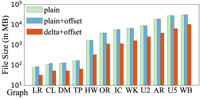
(a) Storage consumption for topology.

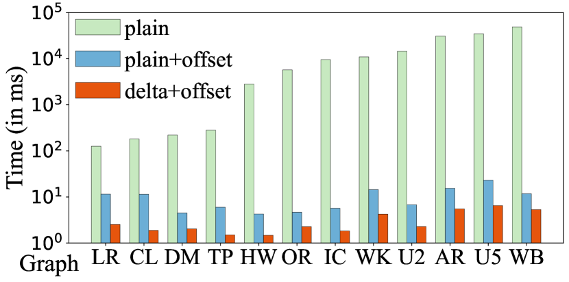
(b) Neighbor retrieval time.

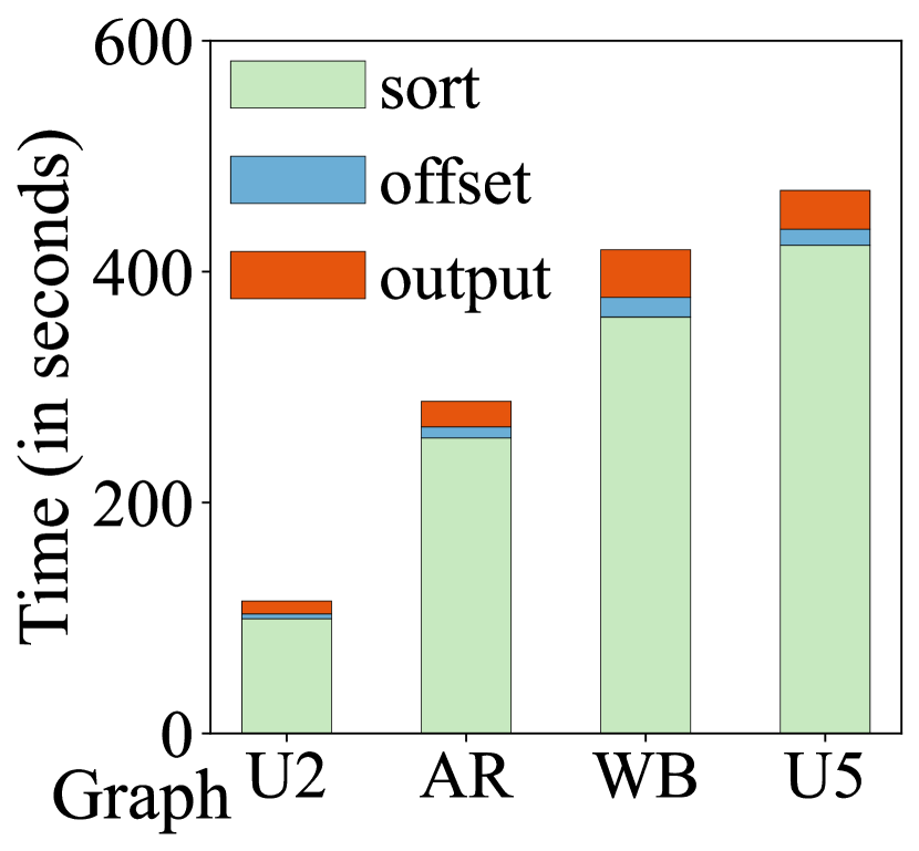
(c) Data transformation time.

Figure 8: Micro-benchmark of neighbor retrieval.

6.2.2 Performance of Neighbor Retrieval

To evaluate GraphAr’s efficiency in neighbor retrieval, we query vertices with the largest degree in selected graphs, maintaining edges in CSR-like or CSC-like formats depending on the degree type. Figure 8(b) shows that GraphAr significantly outperforms the baselines, achieving speedups ranging from $49.8\times$ to $9232.4\times$ over the “plain” method and $2.1\times$ to $6.1\times$ over the “plain + offset” baseline. These gains are attributed to the offset integration and delta encoding, as well as our proposed BMI-based decoding strategy. The offset integration alone accounts for a speedup of between $11.0\times$ and $4177.2\times$, and delta encoding contributes an additional $1.8\times$ to $3.6\times$ speedup on top of that. While not explicitly shown in the log-scaled Figure 8(b), the use of BMI and SIMD further enhances performance, with an average improvement of $20.1\%$.

6.2.3 Performance of Data Transformation

Given that GraphAr is designed for storing LPGs in data lakes, the efficiency of converting original graph data into the GraphAr format is crucial. We focus on the time required for this transformation, using four large graphs (U2, AR, WB and U5) represented as Arrow Tables, a standardized in-memory format in big data systems. Since graphs generally have significantly more edges than vertices and GraphAr employs CSR/CSC-like layouts requiring edge sorting, generating topological data becomes the most time-intensive part.

To dissect this time overhead, we perform a breakdown analysis in Figure 8(c), which shows that we can generate topological data for over $3.9$ million edges per second. The process involves three steps: 1) sorting the edges using Arrow/Acero’s internal order_by operator, labeled as “sort”; 2) generating vertex offsets, labeled as “offset”; and 3) writing the sorted and offset data into Parquet files with specific encoding, labeled as “output”. Generally, this process has a time complexity of $O(|E|log|E|)$ sequentially. Considering this transformation is a one-time, offline operation that substantially reduces future data retrieval times, the associated overhead is acceptable. The most time-consuming step, sorting, offers room for further optimization through distributed frameworks like Spark.

6.3 Micro-Benchmark of Label Filtering

This section evaluates GraphAr’s efficiency in storing and filtering vertex labels. We employ datasets from OGB [39] and Neo4j [14], which feature property graphs with multiple vertex labels, with the number of labels (ranging from $3$ to $349$) indicated under the graph name in Figure 9(a).

6.3.1 Storage Efficiency

We assess storage efficiency by measuring the size of encoded Parquet files used for storing vertex labels. Two baseline methods serve for comparison: The first, termed “string,” concatenates all labels of a vertex into a single string column using BYTE_ARRAY datatype and plain encoding. The second, named “binary (plain),” represents each label in a separate binary column using BOOLEAN datatype and plain encoding. Our approach, denoted as “binary (RLE),” further optimizes this by utilizing Run-Length Encoding (RLE).

As shown in Figure 9(a), our RLE-based method substantially outperforms the baselines, requiring on average only $2.9\%$ and $10.1\%$ of the storage space compared to the “string” and “binary (plain)” methods, respectively. While Parquet does support dictionary encoding that could potentially enhance the “string” baseline, we excluded this from our evaluation. The reason being that, despite some storage gains, dictionary encoding incurs a decoding slowdown of up to $10\times$ due to the extra overhead of storing the dictionary, especially when label numbers are high. Our RLE-based strategy strikes a balance between storage efficiency and decoding performance, as demonstrated in the subsequent experiments.

6.3.2 Performance of Simple Condition Filtering

Recognizing that filtering based on simple conditions represents the cornerstone operation in graph query languages, we prioritize evaluating this operation. For each graph, we perform experiments where we consider each label individually as the target label for filtering, and determine the vertices with that label. To ensure accuracy, each experiment is repeated for $100$ times and the total execution time is reported.

Figure 9(b) illustrates the results, demonstrating that the GraphAr method significantly improves the performance of label filtering based on simple conditions. The most straightforward approach, “string”, which involves decoding the string of labels and conducting matching for each vertex, is the slowest. The “binary (plain)” method separates labels into individual columns and utilizes a binary representation, while the ‘binary (RLE)” method further optimizes the encoding by using RLE. However, both of these methods still require evaluating each vertex. In contrast, our method, referred to as “binary (RLE) + interval”, simply selects all satisfied intervals.

In Figure 9(b), for each graph, we report the middle value of the execution time among filtering each label as the height of the bar, with the error bar representing the range of execution time. Our method may have a large range on some graphs (AX, MA) due to the varying encoding efficiency (i.e., the number of intervals generated) for different columns. However, since the number of intervals is not larger than the number of vertices in any case, our method consistently outperforms the baselines. On average, it achieves a speedup of $6.0\times$ over the “string” method, $3.3\times$ over the “binary (plain)” method, and $2.3\times$ over the “binary (RLE)” method.

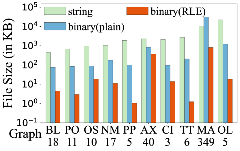
(a) Storage consumption for labels.

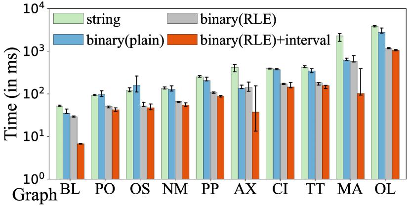
(b) Simple condition filtering.

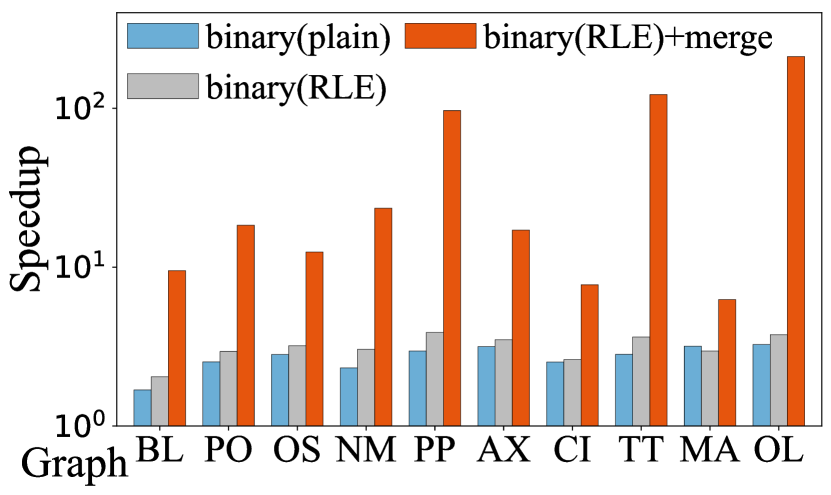
(c) Complex condition filtering.

Figure 9: Micro-benchmark of label filtering.

6.3.3 Performance of Complex Condition Filtering

We also assess the performance of label filtering based on complex conditions using the same graphs as mentioned above. For graphs obtained from Neo4j, we first refer to the provided documentation to identify a filtering operation that involves two labels. If not provided, we create a condition by combining two related labels using either the logical AND operator (if there are vertices satisfying the condition) or OR (otherwise) to reflect real-world semantics. For graphs obtained from OGB, we utilize the first two labels and combine them using OR as the filtering condition.

Figure 9(c) presents the speedup of different methods against the most straightforward approach (referred to as “string” in Figure 9(a) and Figure 9(b)). The results demonstrate that GraphAr performs the best for all test cases. Further analysis reveals that the performance improvement is attributed to the binary representation (as observed in the comparison between “binary (plain)” and “string”), and utilization of RLE (as seen in the comparison between “binary (RLE)” and “binary (plain)”). However, the most significant improvement comes from the merge-based decoding, as observed in the comparison between “binary (RLE) + merge” and “binary (RLE)”, which results in a further speedup of up to $56.3\times$.

6.3.4 Scale Up the Number of Labels

Figure 10 illustrates the execution time of filtering conditions with varying numbers of labels, focusing on BL and MA, which are selected from different datasets (Neo4j and OGB) and have a relatively large number of labels. We test the filtering with $i$ labels by combining the first $i$ labels in a graph using the OR operator as the condition, to ensure that there are vertices satisfying the condition. To reduce experimental noise, we conduct the experiments for $100$ times and report the total execution time for BL and the average time for MA.

As shown in the figure, GraphAr consistently outperforms others on BL. While on MA, it performs best when the number of involved labels is no more than $40$. As the number of labels continuously increases, it performs worse than the baseline “binary (RLE)”, which is due to the number of merged intervals also increasing. In the worst case, the UDF is called for each vertex, means any two consective vertices have different labels. Considering the overhead of merging intervals from different columns, our method may perform worse than directly evaluating the UDF for each vertex. Fortunately, our investigation of real-world workloads reveals that the number of filtered labels in user-written queries is often limited. For instance, in the documentation of Neo4j examples  [14], the filtering involves no more than $5$ labels. Consequently, the performance of our method remains highly promising.

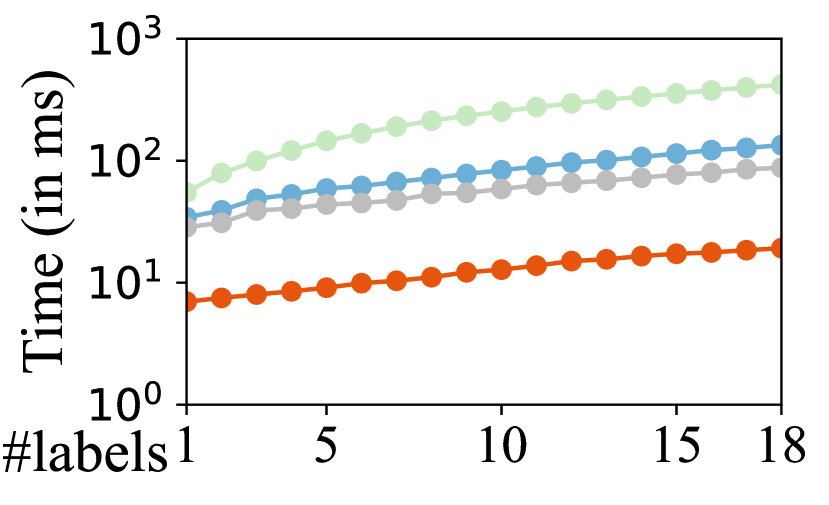
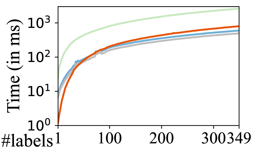
Figure 10: Execution time with the number of labels increases on, tested on BL (left) and MA (right).

6.4 Storage Media

We assess the efficiency of GraphAr across various storage media: local in-memory tmpfs, ESSD (an Alibaba Cloud virtualized elastic block device), and S3-like Object Store Service (OSS). The graph used is SF100, with specifically foucus on the comment vertex type and comment_hasTag_tag edge type.

Table 2 encapsulates the efficiency of GraphAr across different storage media. These results conclusively establish that GraphAr is not only efficient but also robust, delivering consistently high performance, with speedups of $88\times$ to $154\times$ for neighbor retrieval and $2.7\times$ to $11\times$ for label filtering.

6.5 End-to-end Workloads

To demonstrate the practicality of GraphAr in real-world scenarios, we conduct a performance evaluation using end-to-end workloads from the LDBC SNB benchmark [32, 57], which is widely used in the graph processing community. Although the benchmark specifies vertex/edge types, it does not explicitly define the labels. However, we are able to identify certain vertex types that are static (e.g., tagclass and place), which have a fixed and very small vertex set size that does not scale with the graph size. On the other hand, vertex types like comment and person are considered dynamic. Based on this observation, we can treat information related to static types as labels for dynamic types in GraphAr, for example, all tag classes of a comment are attached as labels for the corresponding comment vertex. Similar strategies are also adopted by graph databases [37] to optimize data access performance.

For evaluation, graphs at different scales (listed in Table 1) are generated using the LDBC SNB data generator, as Parquet files. These graphs are then converted into GraphAr format, with the vertex labels attached as described above. Upon investigating the benchmark, including $7$ short and $14$ complex interactive queries, as well as $20$ business intelligence queries, we find that neighbor retrieval is frequently encountered, involved in approximately $90\%$ of the queries. Considering the aforementioned label organization, label filtering is also common, involved in approximately $50\%$ of the queries.

Table 2: Performance comparison across storage media.

	Neighbor Retrieval (s)		Label Filtering (s)
Storage	Plain	GraphAr	String	GraphAr
tmpfs	6.446	0.053	3.984	1.489
ESSD	16.41	0.106	19.06	1.746
OSS	189.4	2.145	252.8	26.22

6.5.1 Query Implementations

Queries. The evaluation focuses on three representative queries, with the required parameters set according to the reference implementations [12, 11]. The first query, IS-3 (interactive-short-3), aims to find all the friends of a given person and return their information. It exemplifies the common pattern of querying neighboring vertices and retrieving associated properties. The second query, IC-8 (interactive-complex-8), is more complex as it involves traversing multiple hops from the starting vertex. Lastly, the BI-2 (business-intelligence-2) query aims to analyze tag evolution. It involves finding and counting the messages associated with tags within a specific tag class, thus requiring vertex filtering by labels.

GraphAr. We develop hand-written implementations for each query based on GraphAr, which utilize the data organization and specifically prioritize two essential operations: neighbor retrieval and label filtering. Our implementation refers to the official reference implementations [12, 11] in Cypher or SQL, to ensure equivalence to the original queries.

Acero. We also implement these queries in Acero [1], which is a powerful C++ library integrated into Apache Arrow for analyzing large streams of data. It offers a comprehensive set of operators such as scan, filter, project, aggregate, and join, among others. Moreover, Acero supports taking Parquet as the data source and enables the pushdown of predicates, making it a strong baseline for comparison with GraphAr. Despite our best efforts to optimize it, we do not perform data re-organization or utilize GraphAr’s encoding/decoding optimizations for the implementations based on Acero.

6.5.2 Performance Comparison

Table 3 presents a comparison of end-to-end time performance, demonstrating that the implementation based on GraphAr significantly outperforms Acero, achieving an average speedup of $29.5\times$. Upon closer examination of the results, it becomes apparent that the performance improvement can be attributed to the following factors: 1) data layout design and encoding/decoding optimizations we proposed, to enable efficient neighbor retrieval (IS-3, IC-8, BI-2) and label filtering (BI-2), as demonstrated in micro-benchmarks; 2) bitmap generation during the two critical operations, which can be utilized in subsequent selection steps (IS-3, IC-8, BI-2).

Taking IS-3 as an example, the optimization of neighbor retrieval achieves an average speedup of $571.4\times$ compared to the baseline utilizing Parquet’s filter pushdown. The subsequent selection based on bitmaps provides a speedup of $2.7\times$. Other steps like order_by show similar performance in GraphAr and Acero due to closely matched implementations.

Table 3: Execution time for IS-3, IC-8 and BI-2 (in seconds).

Graph	SF30		SF100		SF300
Impl.	Acero	GraphAr	Acero	GraphAr	Acero	GraphAr
IS-3	0.156	0.005	0.475	0.010	1.390	0.029
IC-8	72.22	3.362	245.5	6.563	894.4	23.29
BI-2	67.74	4.295	231.6	16.28	755.6	50.04

Summary. In the comprehensive evaluation, GraphAr has been demonstrated to be a highly effective storage scheme for LPGs in data lakes. The key takeaways are:

• Storage efficiency: GraphAr remarkably reduces storage requirements, using only $27.3\%$ of the storage compared to baseline methods for storing topology, and as low as $2.9\%$ for label storage on average.

• Query performance: GraphAr significantly outpaces the baselines in retrieval time, achieving speedups ranging from $49.8\times$ to $9232.4\times$ for neighbor retrieval and an average speedup of $6.0\times$ for simple label filtering, as observed in micro-benchmarks on the ESSD storage.

• Storage media: Preliminary evaluations indicate seamless compatibility across various storage layers like local in-memory tmpfs, ESSD, and S3-like Object Store Service (oss), all achieving high speedup of $88\times$ to $154\times$ for neighbor retrieval and $2.7\times$ to $11\times$ for label filtering.

• Real-world relevance: In end-to-end workloads using the LDBC SNB benchmark, GraphAr shows an average speedup of $29.5\times$ over the Acero baseline, substantiating its practical utility in real-world scenarios.

Collectively, these results validate GraphAr as a robust, storage-efficient, and high-performance solution for both academic research and industrial applications.

7 Related Work

File formats in data lakes. The data lake ecosystem encompasses various common file formats, including CSV, JSON, Protocol Buffers, HDF5 [18], AVRO [3], ORC [4], and Parquet [5]. While these formats support various optimizations that benefit both tables and graphs, they do not inherently cater to some unique needs of LPGs, thus fall short in representing LPG semantics and supporting graph-specific operations.

Data management in data lakes. The popularity of data lakes has led to efforts aimed at enhancing their architecture and data management [48, 25, 16, 54, 49]. These endeavors primarily focus on managing existing data within data lakes and are distinct from GraphAr. GraphAr, on the other hand, can be considered as a new storage format with unique features. It can be leveraged by these existing works to further extend the utility and capabilities of data lakes.

Graph file formats. There are specific formats designed for graph data [27, 38, 9, 24] and RDF (Resource Description Framework) data [17, 46]. However, the primary focus of these formats is to describe or exchange graph data in a standardized manner, e.g., utilizing XML, and are not optimized for storage and retrieval purposes. The lack of encoding, compression and push-down optimizations can lead to far inferior performance, making them less suitable for managing LPGs in data lakes.

Graph databases. There are also graph databases [13, 31, 10] that are designed to store and manage graph data. While they offer various features that are tailored for LPGs, they primarily focus on in-memory mutable data management, operating at a higher level compared to GraphAr. GraphAr, with its format compatible with the LPG model, can be utilized as an archival format for graph databases.

Operation pushdown. Some previous works [45, 60, 61, 62, 63, 6] aim to develop high-performance operators on storage formats of either column-oriented or row-oriented. These works and GraphAr share the same goal of improving pushdown operators and making the utilization of available CPU instructions. However, it is important to note that these works focus on operations related to relational data, such as scan, select, and filter based on properties. In contrast, GraphAr specifically focuses on two graph-specific operations.

8 Conclusion

In conclusion, this paper introduces GraphAr as an efficient and specialized storage scheme for graph data in data lakes. GraphAr focuses on preserving LPG semantics and supporting graph-specific operations, resulting in notable performance improvements in both storage and query efficiency over existing formats designed for relational tables. The evaluation results validate the effectiveness of GraphAr and highlight its potential as a crucial component in data lake architectures.

References

- [1] Acero: A C++ streaming execution engine. https://arrow.apache.org/docs/cpp/streaming_execution.html.
- [2] Apache Arrow. https://arrow.apache.org/.
- [3] Apache AVRO. https://avro.apache.org/.
- [4] Apache ORC. https://orc.apache.org/.
- [5] Apache Parquet. https://parquet.apache.org/.
- [6] AWS S3 Select. https://aws.amazon.com/cn/blogs/aws/s3-glacier-select/.
- [7] Cypher Query language. https://neo4j.com/developer/cypher/.
- [8] Export Neo4j Data to CSV. https://neo4j.com/labs/apoc/4.4/export/csv/.
- [9] GEXF File Format. https://gexf.net/.
- [10] JanusGraph: an open-source, distributed graph database. https://janusgraph.org/.
- [11] LDBC SNB Business Intelligence (BI) workload implementations. https://github.com/ldbc/ldbc_snb_bi.
- [12] LDBC SNB Interactive workload implementations. https://github.com/ldbc/ldbc_snb_interactive_impls.
- [13] Neo4j Graph Database and Analytics. https://neo4j.com/.
- [14] Neo4j Graph Examples. https://github.com/neo4j-graph-examples.
- [15] Neo4j Spark Connector. https://neo4j.com/docs/spark/current/reading/.
- [16] PuppyGraph: A Cloud-Native Graph Data Lakehouse. https://puppygraph.com/.
- [17] RDF Formats. https://www.w3.org/TR/.
- [18] The HDF5 Library and File Format. https://www.hdfgroup.org/solutions/hdf5/.
- [19] Information technology – Database languages – SQL, June 2023. ISO/IEC 9075:2023.
- [20] Renzo Angles, Angela Bonifati, Stefania Dumbrava, George Fletcher, Alastair Green, Jan Hidders, Bei Li, Leonid Libkin, Victor Marsault, Wim Martens, et al. Pg-schema: Schemas for property graphs. Proceedings of the ACM on Management of Data, 1(2):1–25, 2023.
- [21] Dmitry Anikin, Oleg Borisenko, and Yaroslav Nedumov. Labeled property graphs: Sql or nosql? In 2019 Ivannikov Memorial Workshop (IVMEM), pages 7–13. IEEE, 2019.
- [22] Michael Armbrust, Tathagata Das, Liwen Sun, Burak Yavuz, Shixiong Zhu, Mukul Murthy, Joseph Torres, Herman van Hovell, Adrian Ionescu, Alicja Łuszczak, Michał undefinedwitakowski, Michał Szafrański, Xiao Li, Takuya Ueshin, Mostafa Mokhtar, Peter Boncz, Ali Ghodsi, Sameer Paranjpye, Pieter Senster, Reynold Xin, and Matei Zaharia. Delta lake: High-performance acid table storage over cloud object stores. Proc. VLDB Endow., 13(12):3411–3424, aug 2020.
- [23] Nico Baken. Linked data for smart homes: Comparing rdf and labeled property graphs. In LDAC2020—8th Linked Data in Architecture and Construction Workshop, pages 23–36, 2020.
- [24] Vladimir Batagelj and Andrej Mrvar. Pajek—analysis and visualization of large networks. In International Symposium on Graph Drawing, pages 477–478. Springer, 2001.
- [25] Alexander Behm, Shoumik Palkar, Utkarsh Agarwal, Timothy Armstrong, David Cashman, Ankur Dave, Todd Greenstein, Shant Hovsepian, Ryan Johnson, Arvind Sai Krishnan, Paul Leventis, Ala Luszczak, Prashanth Menon, Mostafa Mokhtar, Gene Pang, Sameer Paranjpye, Greg Rahn, Bart Samwel, Tom van Bussel, Herman van Hovell, Maryann Xue, Reynold Xin, and Matei Zaharia. Photon: A fast query engine for lakehouse systems. In Proceedings of the 2022 International Conference on Management of Data, SIGMOD ’22, pages 2326–2339, New York, NY, USA, 2022. Association for Computing Machinery.
- [26] Paolo Boldi and Sebastiano Vigna. The webgraph framework i: compression techniques. In Proceedings of the 13th international conference on World Wide Web, pages 595–602, 2004.
- [27] Ulrik Brandes, Markus Eiglsperger, Ivan Herman, Michael Himsolt, and M. Scott Marshall. Graphml progress report structural layer proposal. In Petra Mutzel, Michael Jünger, and Sebastian Leipert, editors, Graph Drawing, pages 501–512, Berlin, Heidelberg, 2002. Springer Berlin Heidelberg.
- [28] Benoit Dageville, Thierry Cruanes, Marcin Zukowski, Vadim Antonov, Artin Avanes, Jon Bock, Jonathan Claybaugh, Daniel Engovatov, Martin Hentschel, Jiansheng Huang, Allison W. Lee, Ashish Motivala, Abdul Q. Munir, Steven Pelley, Peter Povinec, Greg Rahn, Spyridon Triantafyllis, and Philipp Unterbrunner. The snowflake elastic data warehouse. In Proceedings of the 2016 International Conference on Management of Data, SIGMOD ’16, pages 215–226, New York, NY, USA, 2016. Association for Computing Machinery.
- [29] Timothy A. Davis and Yifan Hu. The university of florida sparse matrix collection. ACM Trans. Math. Softw., 38(1), dec 2011.
- [30] Alin Deutsch, Nadime Francis, Alastair Green, Keith Hare, Bei Li, Leonid Libkin, Tobias Lindaaker, Victor Marsault, Wim Martens, Jan Michels, Filip Murlak, Stefan Plantikow, Petra Selmer, Oskar van Rest, Hannes Voigt, Domagoj Vrgoč, Mingxi Wu, and Fred Zemke. Graph pattern matching in gql and sql/pgq. In Proceedings of the 2022 International Conference on Management of Data, SIGMOD ’22, pages 2246–2258, New York, NY, USA, 2022. Association for Computing Machinery.
- [31] Alin Deutsch, Yu Xu, Mingxi Wu, and Victor E. Lee. Tigergraph: A native MPP graph database. CoRR, abs/1901.08248, 2019.
- [32] Orri Erling, Alex Averbuch, Josep Larriba-Pey, Hassan Chafi, Andrey Gubichev, Arnau Prat, Minh-Duc Pham, and Peter Boncz. The ldbc social network benchmark: Interactive workload. In Proceedings of the 2015 ACM SIGMOD International Conference on Management of Data, SIGMOD ’15, pages 619–630, New York, NY, USA, 2015. Association for Computing Machinery.
- [33] Avrilia Floratou, Umar Farooq Minhas, and Fatma Özcan. Sql-on-hadoop: Full circle back to shared-nothing database architectures. Proceedings of the VLDB Endowment, 7(12):1295–1306, 2014.
- [34] Nadime Francis, Amelie Gheerbrant, Paolo Guagliardo, Libkin Leonid, Victor Marsault, Wim Martens, Filip Murlak, Liat Peterfreund, Alexandra Rogova, and Domagoj Vrgoč. A Researcher’s Digest of GQL. In 26th International Conference on Database Theory (ICDT 2023), volume 255, Ioannina, Greece, March 2023.
- [35] Nadime Francis, Alastair Green, Paolo Guagliardo, Leonid Libkin, Tobias Lindaaker, Victor Marsault, Stefan Plantikow, Mats Rydberg, Petra Selmer, and Andrés Taylor. Cypher: An evolving query language for property graphs. In Proceedings of the 2018 International Conference on Management of Data, SIGMOD ’18, pages 1433–1445, New York, NY, USA, 2018. Association for Computing Machinery.
- [36] Joseph E Gonzalez, Reynold S Xin, Ankur Dave, Daniel Crankshaw, Michael J Franklin, and Ion Stoica. Graphx: Graph processing in a distributed dataflow framework. In 11th USENIX Symposium on Operating Systems Design and Implementation (OSDI 14), pages 599–613, 2014.
- [37] Pranjal Gupta, Amine Mhedhbi, and Semih Salihoglu. Columnar storage and list-based processing for graph database management systems. Proc. VLDB Endow., 14(11):2491–2504, jul 2021.
- [38] Michael Himsolt. Gml: A portable graph file format. 2010.
- [39] Weihua Hu, Matthias Fey, Marinka Zitnik, Yuxiao Dong, Hongyu Ren, Bowen Liu, Michele Catasta, and Jure Leskovec. Open graph benchmark: Datasets for machine learning on graphs. arXiv preprint arXiv:2005.00687, 2020.
- [40] Todor Ivanov and Matteo Pergolesi. The impact of columnar file formats on sql-on-hadoop engine performance: A study on orc and parquet. Concurrency and Computation: Practice and Experience, 32(5):e5523, 2020.
- [41] Pwint Phyu Khine and Zhao Shun Wang. Data lake: a new ideology in big data era. In ITM web of conferences, volume 17, page 03025. EDP Sciences, 2018.
- [42] Jérôme Kunegis. Konect: The koblenz network collection. In Proceedings of the 22nd International Conference on World Wide Web, WWW ’13 Companion, page 1343–1350, New York, NY, USA, 2013. Association for Computing Machinery.
- [43] D. Lemire and L. Boytsov. Decoding billions of integers per second through vectorization. Software: Practice and Experience, 45(1):1–29, may 2013.
- [44] Jure Leskovec and Andrej Krevl. SNAP Datasets: Stanford large network dataset collection. http://snap.stanford.edu/data, June 2014.
- [45] Yinan Li, Jianan Lu, and Badrish Chandramouli. Selection pushdown in column stores using bit manipulation instructions. Proceedings of the ACM on Management of Data, 1(2):1–26, 2023.
- [46] Miguel A. Martínez-Prieto, Mario Arias, and Javier Fernández. Exchange and consumption of huge rdf data. volume 7295, pages 437–452, 05 2012.
- [47] Natalia Miloslavskaya and Alexander Tolstoy. Big data, fast data and data lake concepts. Procedia Computer Science, 88:300–305, 2016.
- [48] Fatemeh Nargesian, Erkang Zhu, Renée J. Miller, Ken Q. Pu, and Patricia C. Arocena. Data lake management: Challenges and opportunities. Proc. VLDB Endow., 12(12):1986–1989, aug 2019.
- [49] Max Neunhöffer. Fishing for graphs in a Hadoop data lake. https://www.oreilly.com/content/fishing-for-graphs-in-a-hadoop-data-lake/.
- [50] Orestis Polychroniou, Arun Raghavan, and Kenneth A. Ross. Rethinking simd vectorization for in-memory databases. In Proceedings of the 2015 ACM SIGMOD International Conference on Management of Data, SIGMOD ’15, page 1493–1508, New York, NY, USA, 2015. Association for Computing Machinery.
- [51] Orestis Polychroniou and Kenneth A. Ross. Towards practical vectorized analytical query engines. In Proceedings of the 15th International Workshop on Data Management on New Hardware, DaMoN’19, New York, NY, USA, 2019. Association for Computing Machinery.
- [52] Orestis Polychroniou and Kenneth A. Ross. Vip: A simd vectorized analytical query engine. The VLDB Journal, 29(6):1243–1261, jul 2020.
- [53] Raghu Ramakrishnan, Baskar Sridharan, John R Douceur, Pavan Kasturi, Balaji Krishnamachari-Sampath, Karthick Krishnamoorthy, Peng Li, Mitica Manu, Spiro Michaylov, Rogério Ramos, et al. Azure data lake store: a hyperscale distributed file service for big data analytics. In Proceedings of the 2017 ACM International Conference on Management of Data, pages 51–63, 2017.
- [54] Franck Ravat and Yan Zhao. Metadata management for data lakes. In New Trends in Databases and Information Systems: ADBIS 2019 Short Papers, Workshops BBIGAP, QAUCA, SemBDM, SIMPDA, M2P, MADEISD, and Doctoral Consortium, Bled, Slovenia, September 8–11, 2019, Proceedings 23, pages 37–44. Springer, 2019.
- [55] Marko A. Rodriguez. The gremlin graph traversal machine and language. CoRR, abs/1508.03843, 2015.
- [56] Ryan A. Rossi and Nesreen K. Ahmed. The network data repository with interactive graph analytics and visualization. In AAAI, 2015.
- [57] Gábor Szárnyas, Jack Waudby, Benjamin A Steer, Dávid Szakállas, Altan Birler, Mingxi Wu, Yuchen Zhang, and Peter Boncz. The ldbc social network benchmark: Business intelligence workload. Proceedings of the VLDB Endowment, 16(4):877–890, 2022.
- [58] Johan Ugander, Brian Karrer, Lars Backstrom, and Cameron Marlow. The anatomy of the facebook social graph. arXiv preprint arXiv:1111.4503, 2011.
- [59] Oskar van Rest, Sungpack Hong, Jinha Kim, Xuming Meng, and Hassan Chafi. Pgql: A property graph query language. In Proceedings of the Fourth International Workshop on Graph Data Management Experiences and Systems, GRADES ’16, New York, NY, USA, 2016. Association for Computing Machinery.
- [60] Thomas Willhalm, Ismail Oukid, Ingo Müller, and Franz Färber. Vectorizing database column scans with complex predicates. 08 2013.
- [61] Thomas Willhalm, Nicolae Popovici, Yazan Boshmaf, Hasso Plattner, Alexander Zeier, and Jan Schaffner. Simd-scan: Ultra fast in-memory table scan using on-chip vector processing units. Proc. VLDB Endow., 2(1):385–394, aug 2009.
- [62] Yifei Yang, Matt Youill, Matthew Woicik, Yizhou Liu, Xiangyao Yu, Marco Serafini, Ashraf Aboulnaga, and Michael Stonebraker. Flexpushdowndb: Hybrid pushdown and caching in a cloud dbms. Proc. VLDB Endow., 14(11):2101–2113, jul 2021.
- [63] Xiangyao Yu, Matt Youill, Matthew Woicik, Abdurrahman Ghanem, Marco Serafini, Ashraf Aboulnaga, and Michael Stonebraker. Pushdowndb: Accelerating a dbms using s3 computation. In 2020 IEEE 36th International Conference on Data Engineering (ICDE), pages 1802–1805, 2020.
- [64] Matei Zaharia, Ali Ghodsi 0002, Reynold Xin, and Michael Armbrust. Lakehouse: A new generation of open platforms that unify data warehousing and advanced analytics. In 11th Conference on Innovative Data Systems Research, CIDR 2021, Virtual Event, January 11-15, 2021, Online Proceedings. www.cidrdb.org, 2021.
- [65] Xiaowei Zhu, Wenguang Chen, Weimin Zheng, and Xiaosong Ma. Gemini: A computation-centric distributed graph processing system. In 12th USENIX Symposium on Operating Systems Design and Implementation (OSDI 16), pages 301–316, 2016.