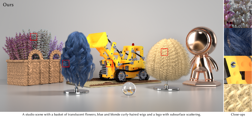
Figure 1. We propose a compact relightable neural 3D asset representation for geometries with complex shading, such as the fiber BCSDF model [Chiang et al., 2016] for blue and blonde curly-haired wigs that exhibit glossy highlights and strong multiple fiber scattering, and the translucent Burley-Christensen shader [Christensen, 2015] combined with shading graphs in the Lego and flowers. Our results are realistic, even at extreme zoom levels, and closely match path-tracing references (shown later). Our representation combines explicit geometry (mesh or fibers) with a neural feature grid and an MLP decoder. This allows for view variation and full relightability, while reducing rendering costs and implementation complexity compared to the original asset representation. The assets can be integrated into a full renderer for path tracing with fast shading under arbitrary lighting conditions, correctly handling light transport within and between assets. On the right we show the close-ups of these assets, demonstrating high-fidelity shading such as complex multiple scattering effects and global illumination.

Relightable Neural Assets

Abstract.

High-fidelity 3D assets with materials composed of fibers (including hair), complex layered material shaders, or fine scattering geometry are critical in high-end realistic rendering applications. Rendering such models is computationally expensive due to heavy shaders and long scattering paths. Moreover, implementing the shading and scattering models is non-trivial and has to be done not only in the 3D content authoring software (which is necessarily complex), but also in all downstream rendering solutions. For example, web and mobile viewers for complex 3D assets are desirable, but frequently cannot support the full shading complexity allowed by the authoring application. Our goal is to design a neural representation for 3D assets with complex shading that supports full relightability and full integration into existing renderers. We provide an end-to-end shading solution at the first intersection of a ray with the underlying geometry. All shading and scattering is precomputed and included in the neural asset; no multiple scattering paths need to be traced, and no complex shading models need to be implemented to render our assets, beyond a single neural architecture. We combine an MLP decoder with a feature grid. Shading consists of querying a feature vector, followed by an MLP evaluation producing the final reflectance value. Our method provides high-fidelity shading, close to the ground-truth Monte Carlo estimate even at close-up views. We believe our neural assets could be used in practical renderers, providing significant speed-ups and simplifying renderer implementations.

1. Introduction

High-fidelity 3D assets with materials using complex layered material shaders (subsurface scattering, coatings, weathered surfaces), or composed of fibers (including hair, fur, or detailed fabrics) are critical in high-end realistic rendering applications. Rendering such models is computationally expensive due to heavy shaders and long scattering paths. Moreover, all downstream renderers need to implement the exact same shading and scattering models as the source authoring system to correctly support the 3D asset. This is non-trivial: for example, web and mobile viewers for 3D assets are unlikely to support the full set of features of advanced 3D content authoring software.

Recent progress in neural rendering suggests converting the 3D asset to a suitable neural representation; however, no existing method provides a sufficient answer. Earlier NeRF representations [Mildenhall et al., 2020; Müller et al., 2022; Chen et al., 2022] focus on view synthesis only; these methods typically bake the original scene lighting into the neural asset, and cannot relight (that is, respond to the illumination of a new scene), which is critical for a high-fidelity asset representation. The spatial resolution of models based on volume rendering is limited: thin primitives like fibers cannot be fully resolved, and close-up views are blurry. However, in our use case the ground-truth geometry is available, and can be used as is, letting us focus on the challenging problem of representing the high-dimensional reflectance accurately.

More recent neural capture methods support relighting [Bi et al., 2020; Sun et al., 2023a; Jin et al., 2023], but this typically works by fitting analytic reflectance models to the observed views, which necessarily degrades complex material appearance. There are some exceptions; the recent work of Zeng et al. [2023] does not have this analytic BRDF limitation, and produces fully neural relightable assets of very high quality from real captures, but still has limitations when representing high-complexity digital 3D assets and does not focus on integrating the results into full-featured renderers. Neural materials [Kuznetsov et al., 2021, 2022] are naturally relightable, but represent standalone materials rather than full assets. We would like to represent the entire asset with its texturing and material assignments, rather than just a flat tileable material patch. Adapting the ideas from the above methods to our asset representation setting is possible, but requires new approaches.

The key contribution of this paper is a neural representation for 3D assets with complex materials that supports high accuracy (even at strong zoom levels), full relightability and correct integration in Monte Carlo path tracers. We keep an explicit geometry, since the cost and implementation complexity of casting primary and shadow rays is reasonable and not a core challenge. Our neural model handles all shading and scattering; no multiple-scattering paths need to be traced, and no complex shaders need to be implemented in the deployment rendering system. Our neural architecture combines an MLP (multi-layer perceptron) decoder with a feature grid, which can be defined using the triplane formulation [Chan et al., 2021]. A shading operation consists of querying the feature vector from the grid at the shading position, followed by passing the feature vector, combined with local information about the geometry intersection, view and light directions, which then produces the final shading color.

Our method provides high fidelity shading, close to the ground truth Monte Carlo estimate even at strong close-up views. Moreover, our assets can be integrated into a full path tracer, interacting correctly with any other scene elements (objects and lights). The data generation consists of rendering $400$ camera views of the asset under different random light directions per pixel, which is tractable even for expensive hair/fur assets. The training on a single NVIDIA A100 ($40GB$) GPU takes about $90$ minutes, with an asset size of about $29MB$ ($30$ minutes and $24MB$ for small model).

In summary, our contributions are:

• A neural 3D representation for assets with complex shading as a combination of explicit geometry, neural feature grid and MLP, allowing for full variation in view and lighting. The representation achieves higher accuracy and rendering performance than previous relightable neural representations.

• An efficient data generation and training pipeline specialized for this representation.

• A full integration of the neural representation into a production renderer. The target renderer can display the asset correctly within a scene consisting of other objects, with full global light transport, at high performance, and with no need to implement the complex material models encoded in the asset.

In the following sections, we cover the background, theory, precomputation, training and rendering of our relightable neural assets, demonstrating high-fidelity renderings, including videos in the supplementary materials.

2. Related Work

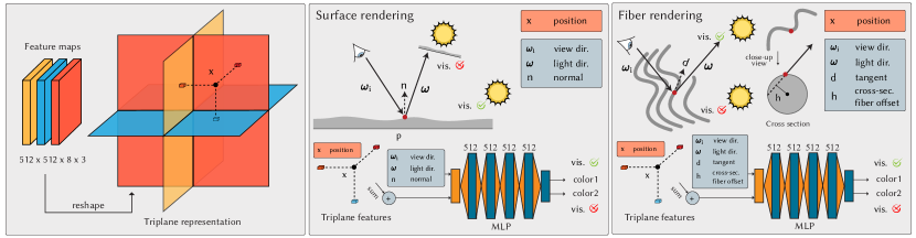
Figure 2. Overview of the pipeline. On the left, we illustrate our triplane representation, consisting of XY, XZ and YZ planes each with 8 feature channels and a default resolution of $512\times 512$. The feature vectors queried from the triplane representation are summed and passed into an MLP, along with additional properties. We show two configuration variants of relightable neural asset pipelines designed for surface rendering (middle) and fiber rendering (right), respectively. The main difference is that surfaces use a normal input, while fibers use tangent and cross-section offset. Both variants output two colors, one of which will be picked according to the visibility at render time.

Ours is a neural relightable rendering method, so we cover neural rendering broadly, and relightable neural capture specifically. Since we target both surface shading and fiber shading, we cover classical techniques in these areas. Additionally, we discuss precomputed radiance transfer (PRT).

Neural rendering in graphics

Recently, deep learning has demonstrated success in a wide range of disciplines, including the field of computer graphics. Neural Radiance Fields (NeRF) [Mildenhall et al., 2020] and follow-up neural scene representations [Chan et al., 2022; Chen et al., 2022; Yu et al., 2021; Müller et al., 2022] enable photorealistic novel view synthesis on complex real-world scenes. However, these neural fields typically do not support relighting, since the lighting and reflectance are baked in the radiance field. Earlier work trained multilayer perceptrons (MLPs) for fast global illumination rendering [Ren et al., 2013, 2015].

Several neural graphics papers targeted specific rendering effects. Kallweit et al. [2017] enables fast cloud rendering with radiance-predicting neural networks. Chu and Thuerey [2017] applied CNNs on efficient fluid simulation. Vicini et al. [2019] learns a shape-adaptive BSSRDF model that better approximates subsurface scattering. Zhu et al. [2021] presented a neural complex luminaire representation that supports the compression, evaluation and importance sampling of the lightfield based on a simplified geometric proxy.

Our work is related to neural materials [Rainer et al., 2019; Kuznetsov et al., 2021, 2022] in its neural architecture and relighting ability, but unlike learning the complex material appearance on planar or curved surfaces, our model is more focused on learning full assets, combining material with geometry. Our approach is similar to the neural architecture of the recent NeuMIP work [2021; 2022], which can theoretically fit any material (e.g. a complex synthetic micro-geometry or measured BTF data) with MLPs.

Relightable neural capture.

Recent advancements in inverse rendering have significantly leveraged neural representations. Various methods, including NeRFactor [Zhang et al., 2021b], Neural Reflectance Fields [Bi et al., 2020], NeRD [Boss et al., 2021a], and TensoIR [Jin et al., 2023], utilize an implicit neural density field for inverse volume rendering, among others [Srinivasan et al., 2021; Boss et al., 2021b; Kuang et al., 2022; Yao et al., 2022; Wu et al., 2023]. Out of these methods, we compare with Bi et al. [2020], because of its high quality (partly due to the dark room capture setup) and its ability to specially handle hair/fur shading.

Alternatively, representing shape via a Signed Distance Field (SDF) is explored in methods such as PhySG [Zhang et al., 2021a], IRON [Zhang et al., 2022a], and more [Zhang et al., 2022b; Mao et al., 2023; Bangaru et al., 2022]. Hybrid methods combining neural and explicit representations with physics-based differentiable rendering are also emerging [Cai et al., 2022; Sun et al., 2023b; Luan et al., 2021; Munkberg et al., 2022; Hasselgren et al., 2022]. However, these methods predominantly depend on analytic BRDF models, limiting their ability to represent and relight complex materials and visual appearances that do not easily fit these models, such as hair, fur, translucency, or skin shading graphs. Deferred Neural Lighting [Gao et al., 2020] inputs proxy geometry and rendered AOVs, employing a 2D CNN decoder for final rendering details. However, it does not support full path tracing integration, as evaluating path throughput for arbitrary positions and ray directions and interleaving path-tracing with CNN passes is non-trivial. NeMF [Zhang et al., 2023] uses a microflake-like phase function instead of a surface BRDF model, but still relies on fitting an analytic parametric material model, inheriting similar limitations.

NRHints [Zeng et al., 2023] is a recent method that overcomes the analytical BRDF constraint, enabling high-fidelity relighting of neural assets from real captured data. However, NRHints involves expensive training and rendering, and did not study full light transport applied to the resulting assets. Representing digital 3D assets with complex geometry and/or multiple scattering is possible with NRHints but less accurate than with our method. In contrast, our method requires significantly less training time, supports full relightability, and achieves full path-tracing integration into existing renderers at real-time frame rates. Of course, our method is designed for representing digital assets while NRHints focuses on capturing real objects; however, NRHints is still the closest alternative method to ours, so we provide extensive comparisons to it.

Complex surface and subsurface shading

Translucency, specifically subsurface scattering (SSS), plays an important role for skin and many other materials. Various shading techniques study efficient simulation of SSS effects [Habel et al., 2013; Donner and Jensen, 2006; Jensen et al., 2001; Donner et al., 2008]. Recently, Monte Carlo random walks [Wrenninge et al., 2017] have been preferred for translucency in high-end production. We use the Burley-Christensen method [Christensen, 2015] but our approach makes no assumptions on the method used to compute the effect in training data. Layered mixture models [Guo et al., 2018; Belcour, 2018; Guo et al., 2016] are capable of faithfully representing complex surface material layering and coating. Lastly, increasing efforts have been made in developing shading languages and material definition tools such as Nvidia MDL, MaterialX, and Adobe Substance. The complexity of materials achievable in a system that allows combining all of these tools using large shading graphs can become intractable for downstream deployment of the assets. A neural representation like ours helps to limit this complexity to the precomputation stage, and produces assets that are much easier to render downstream.

Hair, fur and fabrics are crucial components in representing realistic appearance in our world. Marschner et al. [2003] proposed a realistic hair reflectance model by representing hair fibers as rough dielectric cylinders with reflectance, absorption and transmission, which was later extended by d’Eon et al. [2011] and Khungurn and Marschner [2017]. Yan et al. [2015] presented an animal fur model that represents the fiber geometry with a double cylinder. Chiang et al. [2016] presented a practical fiber shading model for hair and fur (or other fiber-based materials) that is efficient for production path tracing. We use this model to precompute our fiber-based assets, though any similar model could be used. This model is near-field, meaning it defines a full BSDF for points on the fiber, allowing reflectance to vary across the width of the fiber; an important effect that we fully capture. Dual scattering [2008] accounts for the multiple fiber scattering effects in human hair with fast global and local approximations, but requires user intervention in parameter tweaking and only applies to hair.

Precomputed radiance transfer (PRT)

Efficient scene relighting through PRT has been explored in computer graphics research for two decades [Sloan et al., 2002; Ramamoorthi, 2009], often using the spherical harmonic basis, but also using other bases such as wavelets [Ng et al., 2003, 2004], polynomials [Ben-Artzi et al., 2008], spherical Gaussians [Tsai and Shih, 2006; Xu et al., 2013] or neural basis functions [Xu et al., 2022]. It is important to note that the motivation behind PRT methods is fundamentally different from our work. Scenes rendered using PRT are constrained in that they cannot easily incorporate assets that have not undergone the same PRT representation. PRT models do not allow querying the lighting in an arbitrary direction. This lowers the lighting frequencies that can be represented, but even more importantly, the lighting is hard to obtain in a specific basis when shading a given scene point during path tracing. This limitation hinders the compatibility of PRT methods with production Monte Carlo path tracing.

In contrast, our relightable neural assets provide an end-to-end shading solution, which can be seamlessly integrated into existing renderers for Monte Carlo path tracing along with any other classical scene elements for global illumination.

3. Neural Shading Model

Our goal is to take a complex asset and precompute its light transport (including its materials and multiple light interactions with itself) in isolation and compress it using a neural model. Such an asset is fully relightable with respect to the underlying physical light transport and can be inserted into other scenes by quickly evaluating the neural model, for different positions, camera and light directions. No multiple scattering paths need to be traced, and no complex shading models need to be implemented to render our assets, beyond a single neural architecture.

3.1. Relightable Asset Definition

To achieve this, we treat the asset as a scene by itself, lit by some incoming light distribution. The outgoing radiance $L_{o}$ at the shading position $\mathbf{x}_{o}$ with the viewing direction $\bm{\omega}_{o}$ is an integral of the light transport from all positions with all incoming lighting directions

(1) $$L_{o}(\mathbf{x}_{o},\bm{\omega}_{o})=\int_{\mathbf{x}_{i}\in\mathcal{A},\bm{\omega}_{i}\in\bm{\omega}}L_{i}(\mathbf{x}_{i},\bm{\omega}_{i}){T(\mathbf{x}_{o},\bm{\omega}_{o},\mathbf{x}_{i},\bm{\omega}_{i})\mathrm{d}\mathbf{x}_{i}\mathrm{d}\bm{\omega}_{i}},$$

where $L_{i}$ is the incoming radiance at position $\mathbf{x}_{i}$ with lighting direction $\bm{\omega}_{i}$, whose domains are $\mathcal{A}$ and $\bm{\Omega}$ respectively. $T$ is the light transport function from $\{\mathbf{x}_{i},\bm{\omega}_{i}\}$ to $\{\mathbf{x}_{o},\bm{\omega}_{o}\}$, globally depending on the geometries and materials of the entire scene, and including light paths of all lengths.

Representing the above transport would still require 8-dimensional data: each outgoing pair $(\mathbf{x}_{o},\bm{\omega}_{o})$ is an integral over all incoming pairs $(\mathbf{x}_{i},\bm{\omega}_{i})$. We make the further approximation of assuming distant directional light. More precisely, we propose a neural asset $\mathcal{T}$, for which the outgoing radiance is computed as:

(2) $$L_{o}(\mathbf{x},\bm{\omega}_{o})=\int_{\bm{\omega}_{i}\in\bm{\Omega}}L_{i}(\bm{\omega}_{i}){\mathcal{T}(\mathbf{x},\bm{\omega}_{o},\bm{\omega}_{i})\mathrm{d}\bm{\omega}_{i}},$$

where the shading position $\mathbf{x}_{o}$ is denoted as $\mathbf{x}$ for brevity, and $\mathcal{T}$ is defined by integrating out the dependence on $\mathbf{x}_{i}$, that is,

(3) $$\mathcal{T}(\mathbf{x},\bm{\omega}_{o},\bm{\omega}_{i})=\int_{\mathbf{x}_{i}\in\mathcal{A}}T(\mathbf{x}_{o},\bm{\omega}_{o},\mathbf{x}_{i},\bm{\omega}_{i})\mathrm{d}\mathbf{x}_{i}.$$

Equivalently, $\mathcal{T}(\mathbf{x},\bm{\omega}_{o},\bm{\omega}_{i})$ is the radiance leaving $\mathbf{x}$ into direction $\bm{\omega}_{o}$ when lit by a unit-irradiance directional light from direction $\bm{\omega}_{i}$, and including all self-occlusions and inter-reflections. This makes our asset definition similar to a bidirectional texture function (BTF), but defined on an arbitrary geometry instead of a plane. In other words, our assets are akin to 3D BTFs defined over explicit geometry. We show that despite the distant directional light assumption in this definition, our assets can be used with any illumination including near-field lighting, much like BTFs.

Our goal is to represent the asset as a combination of the geometry itself and a neural module capable of evaluating $\mathcal{T}$ for a given shading point $\mathbf{x}$ and given lighting and viewing directions. The similarity of this problem to neural BTF compression also suggests that the design of neural techniques for compressing BTFs could be adapted to our asset compression problem, as we will see shortly.

3.2. Neural Shading Architecture

The neural shading architecture is composed of two steps, as shown in Fig. 2. At a shading point $\mathbf{x}$, we query a feature vector from the triplane feature grid, $\bm{\zeta}(\mathbf{x})$; this feature vector is simply the sum of the features bilinearly interpolated from the three orthographically projected planes (XY, YZ and XZ), similar to Chan et al. [2021].

The shading point $\mathbf{x}$ has other properties, such as the normal (for surface assets), tangent and position along fiber width (for fiber assets). We combine these properties with other available information, such as the camera direction $\bm{\omega}_{o}$, light direction $\bm{\omega}_{i}$. We concatenate all of these properties into a property vector $\tilde{\mathbf{x}}=\tilde{\mathbf{x}}(\mathbf{x},\bm{\omega}_{i},\bm{\omega}_{o})$, which can be thought of as an extended shading point, with all easily available information from the rendering process added to it. More detail on the property vector $\tilde{\mathbf{x}}$ is given below in subsection 3.3. We concatenate $\bm{\zeta}(\mathbf{x})$ and $\tilde{\mathbf{x}}$ into a final input vector $\bm{\xi}$.

In the second step, the transport $\mathcal{T}(\mathbf{x},\bm{\omega}_{i},\bm{\omega}_{o})$ is evaluated by an MLP (multilayer perceptron) decoder taking the concatenation of the feature vector $\bm{\zeta}(\tilde{\mathbf{x}})$ and properties $\tilde{\mathbf{x}}$ as input and returning two RGB colors, one of which will be picked according to the visibility at render time. This design choice is to facilitate the full integration into production renderers — where BSDF evaluation is often done before a shadow ray is traced for visibility. We denote the full input of the MLP as $\bm{\xi}$. The Monte Carlo simulation of global transport is not required any more for runtime evaluation of $\mathcal{T}$, since for any point on the geometry and any incoming and outgoing directions, it can be quickly evaluated through a combination of querying the triplane feature grid and evaluating the MLP.

The neural asset is thus the combination of the geometry, the feature grid $\bm{\zeta}$ and the MLP weights. Once the feature grid and MLP are jointly trained, the scene can be efficiently re-rendered with arbitrary light and camera directions. Importantly, the lighting does not necessarily have to be directional in the final scene where the asset is used, because the neural asset $\mathcal{T}$ is parameterized with the differential of lighting direction $\bm{\omega}_{i}$, similar to other shading models employed in Monte Carlo path tracing. The lighting direction $\bm{\omega}_{o}$ points to a sampled location on any light source and can be different every time $\mathcal{T}$ is evaluated, hence the asset can be used with any lighting that is sampled in a manner similar to traditional Monte Carlo path tracers.

In this sense, our asset is similar to a BTF [Dana et al., 1999], acquired or synthesized under distant directional lighting but used in a final renderer with any lighting (such as area/directional/point emitters and IBLs). Recent neural material representations like NeuMIP [Kuznetsov et al., 2021] are essentially compressed BTFs and make the same assumptions; they are also similar in combining feature grid lookups with MLP decoders, though their MLPs take somewhat different inputs and represent different phenomena on planar surfaces.

In summary, explicit geometry combined with the trained triplane grid $\bm{\zeta}$ and the MLP is a relightable asset that can be evaluated for new camera angles within new illumination conditions.

3.3. Surface Properties

The choice of surface properties $\tilde{\mathbf{x}}$ and $\bm{\xi}$ differs between surface-based and fiber based assets. We append the surface normal $\mathbf{n}(\mathbf{x})$ for surfaces, and direction (tangent) $\mathbf{d}(\mathbf{x})$ for fibers, to the property vector. This is not strictly required, and the model will learn without it, but it improves the fitting accuracy. For fibers, we additionally supply $h(\mathbf{x})$, the offset across the fiber width from the fiber axis, normalized to $[-1,1]$, as introduced by Marschner et al. [2003]. This is critical for the ability of the model to learn spatial variation in lighting across (typically tiny) fiber width, which is a feature of near-field fiber shading models [Chiang et al., 2016].

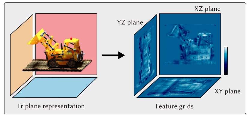
Figure 3. Visualization of the triplane representation. We show the triplane representation for the subsurface lego asset, visualizing the first channel of XY, YZ, and XZ planes, respectively.

Triplane representation

If complete and high-quality UV coordinates are available, our method can use a 2D feature texture, but this is not always feasible. It is challenging to build non-overlapping, low-distortion and compact texture coordinates, especially for meshes with complex topology and fiber assemblies. A more general solution is to use a triplane representation [Chan et al., 2021]. The world position at $\mathbf{x}$ is a $3D$ vector $\{x,y,z\}$, which is converted to three $2D$ vectors of $\{x,y\}$, $\{y,z\}$ and $\{z,x\}$. The neural feature grid $\bm{\zeta}$ is composed of three $2D$ tables for each of them, $\bm{\zeta}_{xy}$, $\bm{\zeta}_{yz}$ and $\bm{\zeta}_{zx}$, as illustrated in Figure 3. Each query outputs an 8-channel vector. By summing the three output vectors, we obtain the final 8-channel feature vector $\bm{\zeta}(\mathbf{x})$.

Lighting Visibility for Self-Shadowing

Direct shadowing is an important effect, easily handled by classical rendering methods, but difficult to learn for a neural network due to its discontinuous nature. Therefore, we also consider the binary visibility of the light direction $\mathbf{V}(\mathbf{x},\bm{\omega}_{i})$, specifying whether the light ray self-intersects with the asset. We use this visibility value as a hint to the MLP, but unlike Zeng et al. [2023] we do not use it as an input, but rather have the MLP produce two outputs (assuming a visibility value of true or false) and pick the right value at render time. This solution provides more practical render integration, as detailed later in Sec. 5. The visibility hint significant improves rendering quality with noise reduction around the shadowing edges.

4. Data Generation and Training

In this section, we describe our data generation pipeline and training details in Sec. 4.1 and Sec. 4.2, respectively.

4.1. Data generation

The training dataset is generated using the Python bindings of Blender 3.5, with a customized CPU version of the Cycles path tracer. Surface scenes are modeled as meshes and can use arbitrary shaders allowed by Blender, including custom shading graphs. For scenes composed of fibers, the fibers are modeled as curved cylinders and their material properties are defined using the model of Chiang et al. [2016], known as Principled Hair BSDF in Blender.

Figure 4 shows our data generation setup along with a visualization of the data generated. To render each image, a perspective camera is randomly placed on a sphere with a user-defined radius centered at the asset, with the field of view set such that the asset is taking most of the view. During data generation, the primary rays within a pixel are all traced through its center, to compute the outgoing radiance of a single visible point $\mathbf{x}$ on the geometry, rather than an average of a footprint. In other words, we are interested in point sampling the appearance spatially, rather than pre-integrating it. Since the primary rays always intersect the same geometry at every pixel, the “alpha” channel of the RGBA rendered result is binary and indicates the pixels that contain valid intersections; these pixels become valid data points for training.

Instead of choosing a single light direction for each image or slice of the training data, we randomize the light direction for each pixel, improving the coverage of the space of view/light pairs available in the dataset. In practice, our path tracer allows lighting to be overridden such that each pixel is rendered with a different light direction $\bm{\omega}_{i}$. As a result, each rendered pixel with a valid intersection provides a separate data point with distinct camera and light directions, which becomes a training sample. Note that even though we use a fixed camera per rendered image in the dataset, it is possible to customize the data generator to produce a random view direction per pixel for shading purposes, just like the light direction. However, we did not find this necessary, and opted for simplicity in keeping the original view directions. Even in this case, the camera directions are slightly different for each pixel since we use a perspective camera, but not random.

In addition to the output radiance, we also utilize a number of arbitrary output variables (AOVs) in the shading graph and output them using Blender’s compositing nodes for the values required by $\tilde{\mathbf{x}}$ and $\bm{\xi}$, such as the position $\mathbf{x}$, viewing direction $\bm{\omega}_{o}$, lighting direction $\bm{\omega}_{i}$ and optionally the lighting visibility $\mathbf{V}$. For an asset composed of fibers, we also output the fiber direction $\mathbf{d}$ and the offset across the fiber $h$.

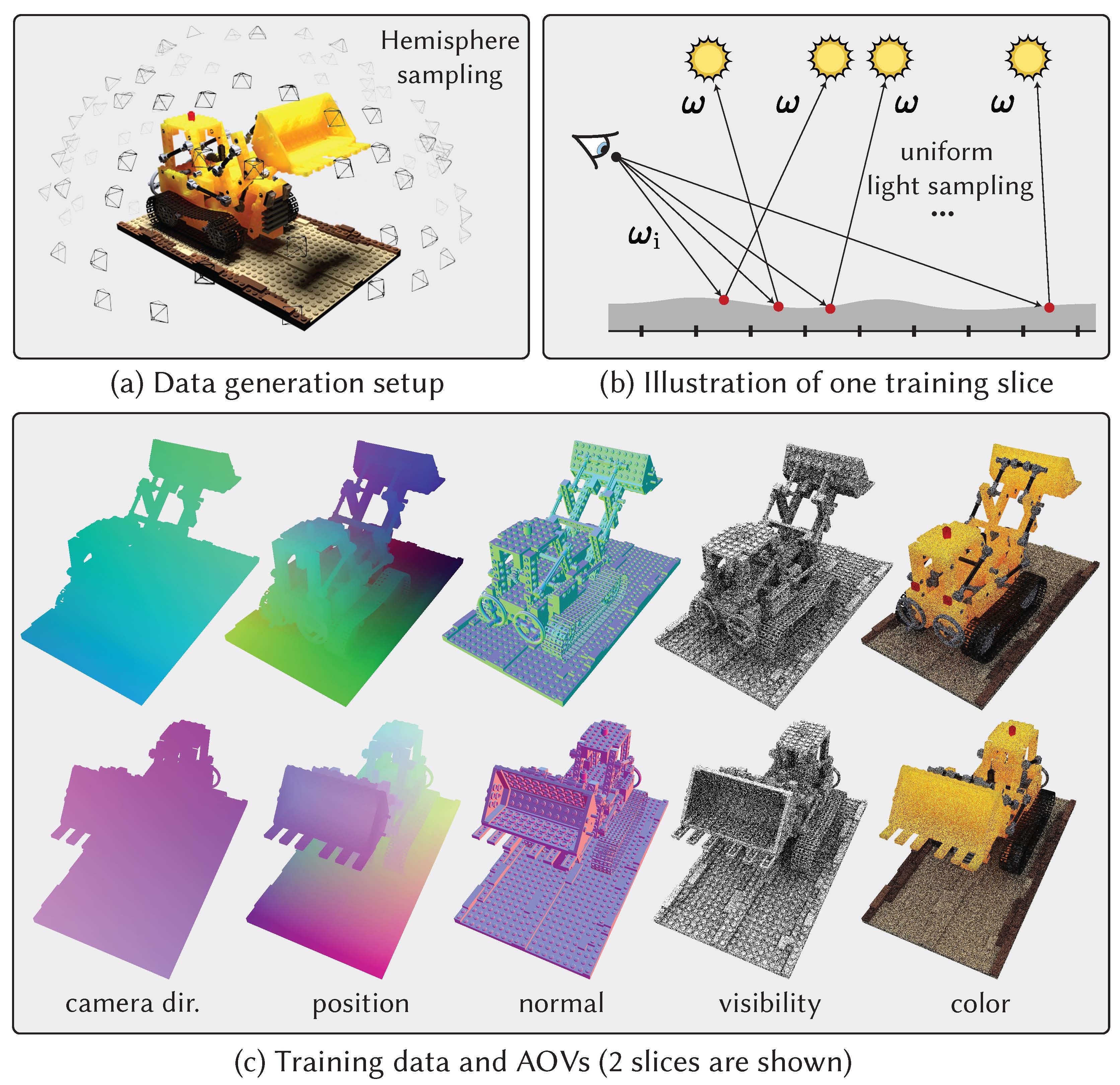
Figure 4. Data generation of our pipeline. (a) We sample camera views around the asset (upper hemisphere) and for each training slice (b) the light directions are randomly sampled for each pixel’s ray hit shading point. In (c), we visualize two slices of the training data and AOVs obtained from Blender Cycles path tracer.

We apply a direct light radiance clamping of value 20.0 and an indirect light clamping of value 10.0. This scales down very bright samples and prevents issues when combining very low roughness and purely directional lighting. Alternatively, we support turning the directional lights into lights with a small angular radius, which also has the same effect of restricting the dynamic range. However, we found that clamping is simpler and works just as well, while making it easier to get accurate visibility hints. Note that previous methods [Zeng et al., 2023; Bi et al., 2020] use low dynamic range images, thus essentially clamping at 1.0.

We render $400$ cameras with a resolution of $1024^{2}$ for a given asset. For some assets, we restrict the lighting directions and viewing directions to the top hemisphere, as it may not be useful to learn bottom hemisphere appearance for certain assets. A typical dataset for a surface asset is about $17.2GB$, while fiber assets increase to about $18GB$. We render $128$ to $4096$ samples per pixel, depending on the complexity of the scattering paths for an asset. Although the rendered data has some remaining noise, it is sufficient as our training regularizes away the noise. We render the images on a cloud instance with $96$ CPU cores. The data for our assets (with complex effects like subsurface scattering and hair with long scattering paths) is generated within $4$ to $6$ hours. We also render out an additional $40$-view validation dataset with fixed light direction per view, enabling us to judge the fitting quality on realistic configurations numerically and visually.

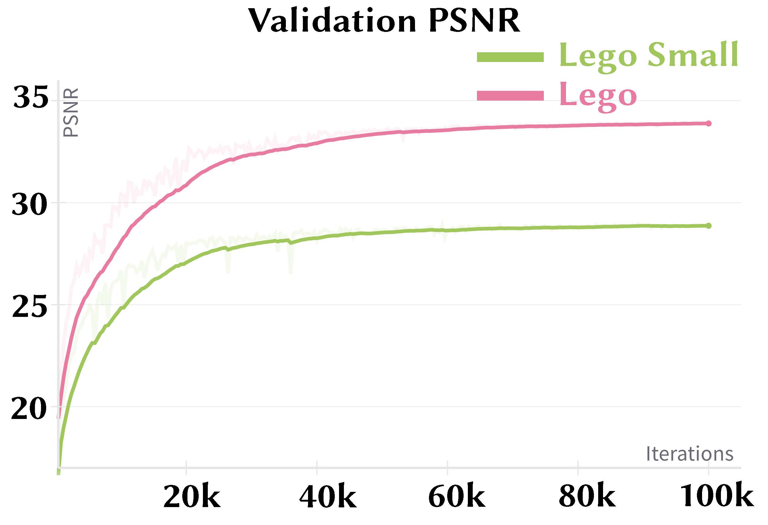
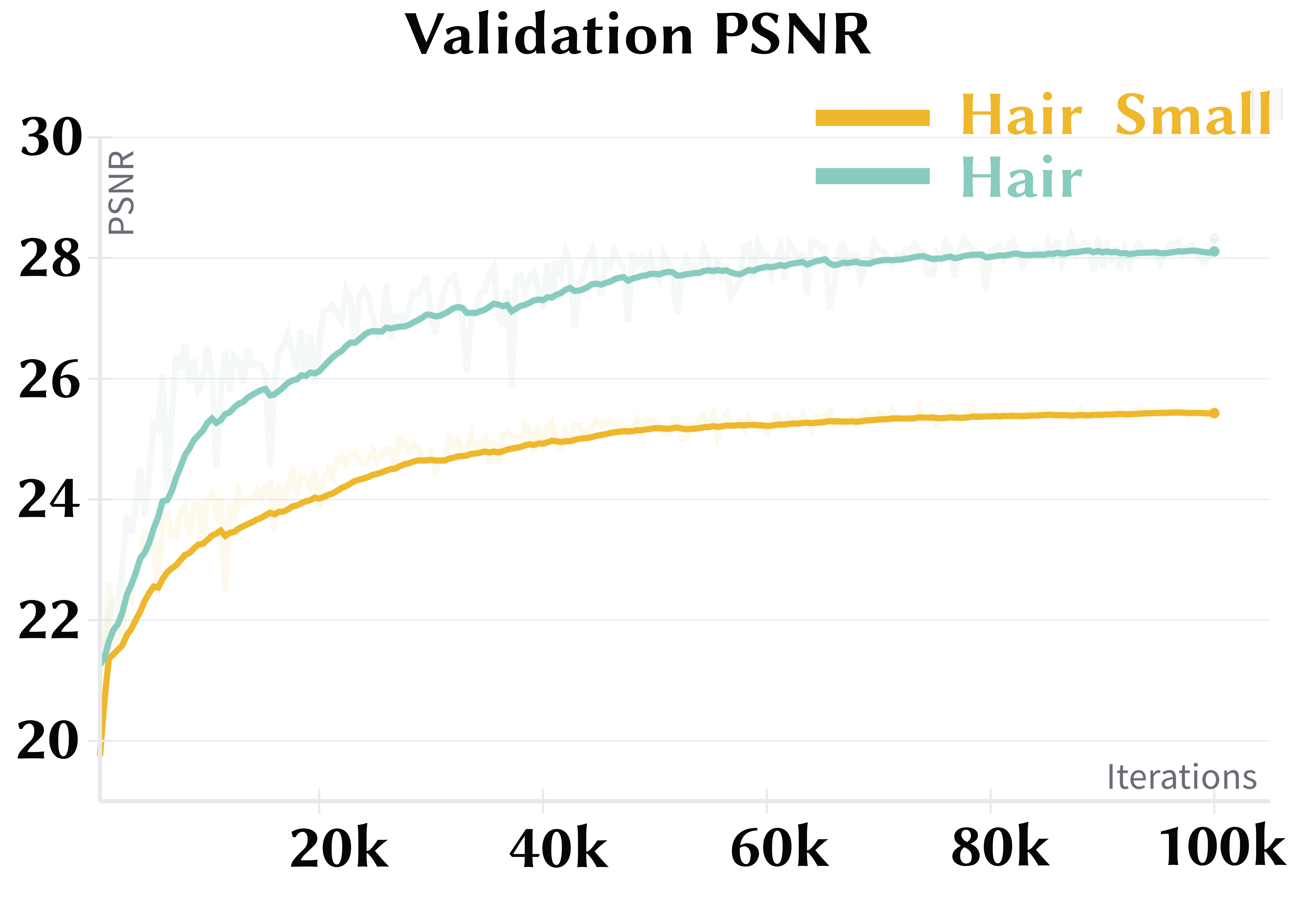
Figure 5. Training convergence plots on translucent lego and blue hair assets. We show the convergence plots for two versions of our model on a surface asset (lego) and a fiber asset (blue hair). The Lego Small and Hair Small are trained with a small variant of our neural model with reduced MLP size for real-time rendering in path tracer, at the cost of compromising some accuracy.

Blender Cycles	Ours	Blender Cycles	Ours (small model)	Ours (small model)	Blender Cycles
(4096 spp, 247 s)	(16 spp, 34 s)	(equal-time, 34 s)	(16 spp, 1.7 s on CPU)	(16 spp, 0.9 s on GPU)	(equal-time, 1 s)

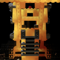
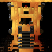
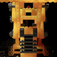
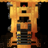
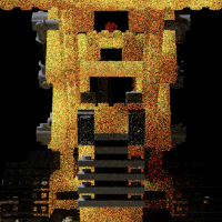
Figure 6. Path tracer integration on surface-based asset. We integrate surface models into a production path tracer on both CPU and GPU rendering. Our model significantly simplfies the shader implementation and improves the rendering performance. In contrast, blender path tracing exhibits severe Monte Carlo noise at equal rendering time budget.

4.2. Training

For each sample point $\mathbf{x}$, the input properties tuple $\bm{\xi}$ is used to predict two RGB transport values $\mathcal{T}$ in the forward pass of our neural architecture. We use the L2 error with $\log(x+1)$ applied to prediction and ground truth, and backpropagate to update the grid $\bm{\zeta}$ and the MLP decoder weights. The network outputs two RGB values (with and without visibility) and we apply the loss only to the output matching the visibility value for the given data point, ignoring the other output.

During training, one batch consists of one image slice from our dataset; each batch contains a different number of valid data samples since every camera can have a different number of valid geometry intersections. As described in 4.1, the ”alpha” channel of the radiance RGBA data is binary; our dataloader only loads data in each image slice with ”alpha” of 1.0, pixels with 0.0 alpha are discarded since they represent ”empty space” with no valid intersections. One training epoch includes the full $400$ batches of data. Our training is implemented using the PyTorch Lightning framework. We use a single Nvidia A100 GPU (40 GB memory) and our entire dataset fits into GPU memory during training, making the training very efficient.

Our training runs for $100,000$ iterations ($250$ epochs) using an Adam optimizer [Kingma and Ba, 2014], along with a StepLR learning rate scheduler using an initial learning rate of $1*10^{-3}$, reducing it by half every $50$ epochs. With these settings, an average training run takes around $90$ to $120$ minutes, and $30$ to $40$ minutes for our small model; so it is much faster than data generation. In contrast, NRHints [Zeng et al., 2023] and Neural Reflectance Fields [Bi et al., 2020] would take roughly a day to train their models on multiple GPUs (e.g. 4).

Note that during the initial iterations of training, we apply a blurring kernel on the three feature grids; starting at an initial footprint of $4$ pixels and gradually decaying it down to $1$ pixel by $20,000$ iterations ($50$ epochs); the remaining training keeps this minimum blur of $1$ pixel. This is inspired by NeuMIP [Kuznetsov et al., 2021] and shows noticeably better results due to spatial low-frequency data sharing, before optimization moves on high frequency details.

During training, we monitor the average PSNR values on the 40 image slices from the validation data set as shown for the Lego and Blue Hair assets in Figure 5. The plots show that the models already converge at around $80,000$ iterations ($200$ epochs), but we notice that letting them train another $20,000$ iterations ($50$ epochs) at the lowest learning rate helps resolve some more high frequency detail.

Blender Cycles	Ours	Blender Cycles	Ours (small model)	Blender Cycles
(4096 spp, 1 hour)	(16 spp, 74.4 s)	(equal-time, 74.6 s)	(16 spp, 17.7 s on CPU)	(equal-time, 17.7 s)

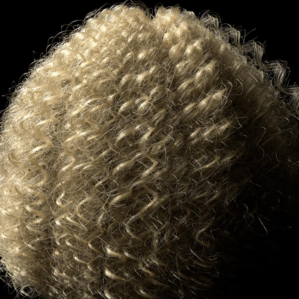
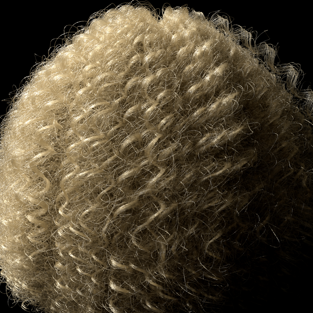
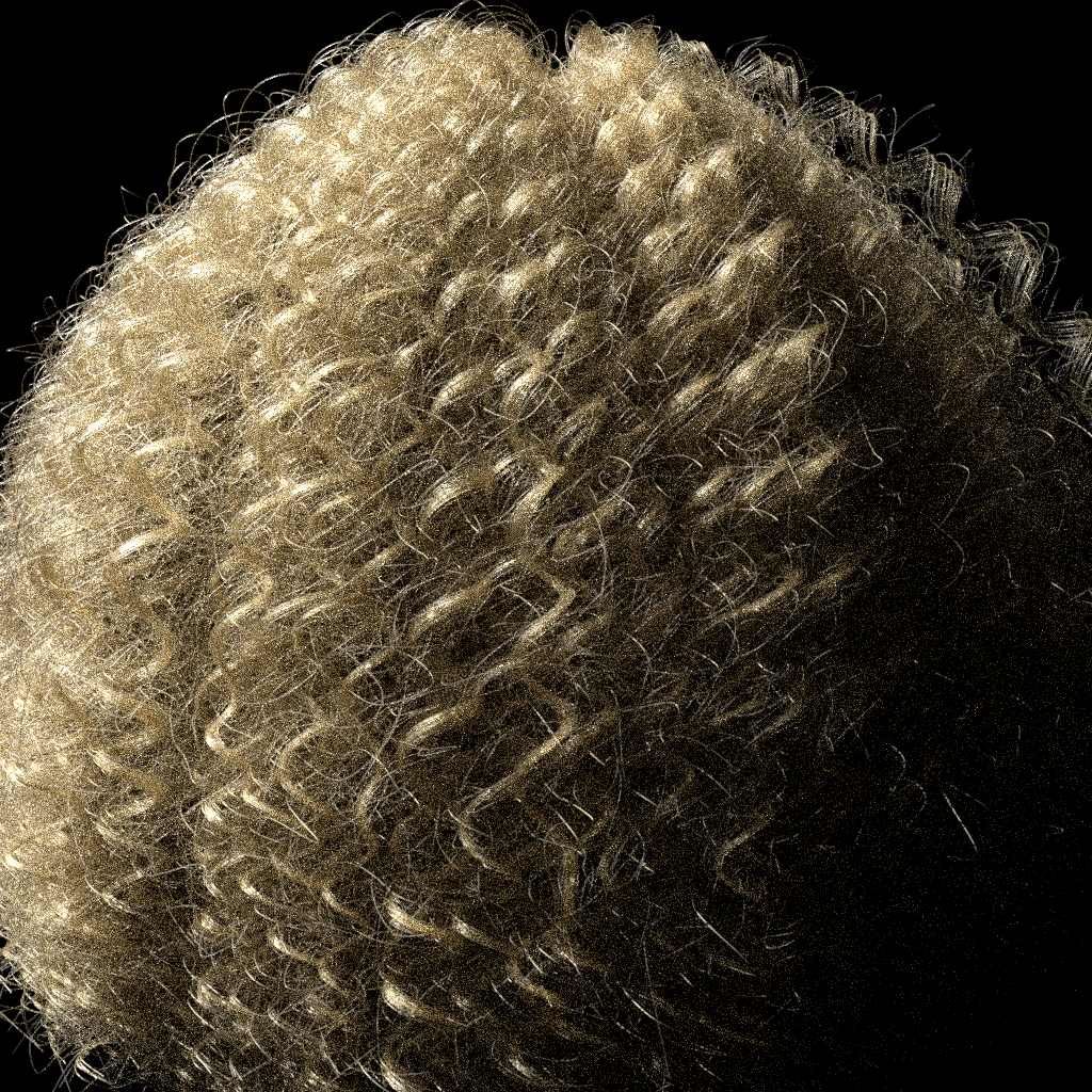
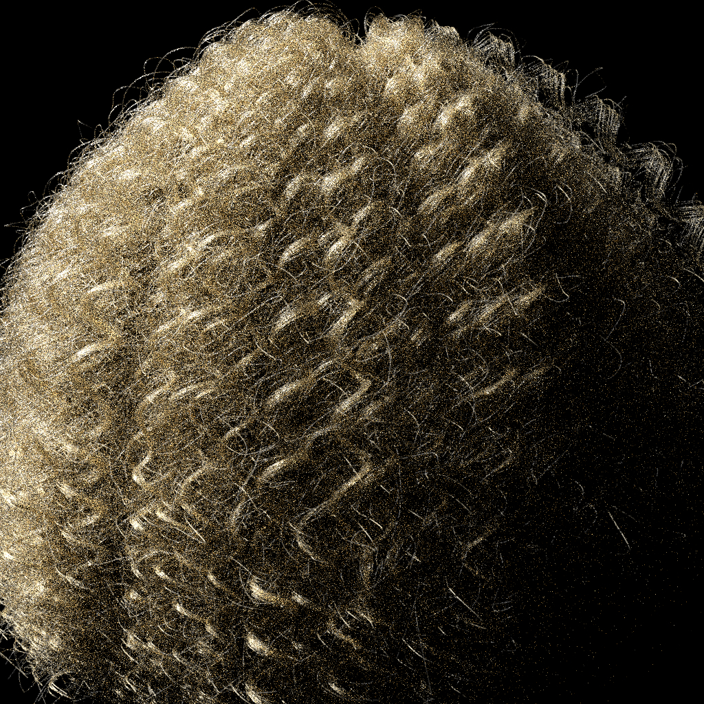
Figure 7. Path tracer integration on fiber-based asset. We integrate hair models into a production path tracer on CPU rendering. Our model significantly simplfies the shader implementation and improves the rendering performance. In contrast, blender path tracing exhibits severe Monte Carlo noise at equal rendering time budget.

We use PyTorch Lightning’s checkpointing system to save out the three best models in terms of PSNR values on the validation dataset as well as the last checkpoint. The trained model includes $7.4$ million parameters ($6.3M$ for small model) between the feature grids and MLP weights, and the total uncompressed size is about $29MB$ ($25MB$ for small model).

5. Rendering

The relightable neural asset can be integrated within a full-featured production path tracer. We demonstrate an integration of our asset in a path tracer that allows for environment (IBL) lighting, local area lighting, other geometries in the scene, and global illumination (Figure 1, 6, 7, 11 and 12).

If a ray intersects the geometry, the shading on the neural asset is computed according to Eq. 2. The original materials are not needed; the neural asset is fully defined by its geometry, feature triplane and MLP weights. Anti-aliasing is applied as usual in the renderer, as our assets encode point-wise rather than pixel-aggregated transport. A rasterizer integration may be possible as well, but we have not studied it yet.

Rendering with a point or directional light simply requires a feature grid query and an MLP evaluation for each hit point. For other illuminations, Monte Carlo light sampling can be used. Indirect rays can be traced from our asset as well, currently based on uniform sampling. Neural importance sampling could be applied in the future, by adapting some of the methods discussed by Xu et al. [2023]. We combine the light samples and indirect samples using multiple importance sampling (MIS).

The implementation needs to take care to recreate the same conditions that the asset has been trained in. All vectors need to be converted to training space (normally equivalent to object space) since this is what the neural model will assume.

Below, we discuss some subtleties of integrating our neural assets into a production path tracer that may not be immediately obvious. Figure 6 and 7 show the correctness of our path tracer integration by comparing to ground truth renders generated using Blender Cycles.

Visibility hint application

In production renderers, BSDF evaluation is frequently done before a shadow ray is traced for the shading point. For example, in frameworks like OptiX and Vulkan raytracing, BSDF evaluation is normally done in a closest hit shader, while visibility checking requires a subsequent ray generation shader to construct the appropriate shadow rays, and the ordering of these shaders would be very tedious to change. Our model essentially replaces the BSDF evaluation in the shading pipeline, so the visibility being unknown at this point is a practical obstacle. To resolve this efficiently, we designed our MLP to output both values (shadowed and unshadowed); we simply hold on to the two values on the ray payload and pick one of these values later on based on the results of the visibility checking.

If the visibility hint is used as an additional MLP input, such as in the assets produced by Zeng et al. [2023], we can still use this approach, though at the cost of double shading cost: we can evaluate the MLP twice for both cases, put the values on the ray payload and continue as above.

Correct light transport handling

The neural representation $\mathcal{T}$ models all transport within the asset; multi-bounce Monte Carlo simulation is only required for the transport between different assets. A shadow ray or a secondary indirect ray should not be occluded by the asset itself, but still intersects the geometries of other assets to allow for inter-asset global transport in the scene.

In practice, for both rays (shadow and indirect), self-intersection is tracked by comparing the instance ID (unique per asset) on the origin of the ray to the ID on the hit point. If a hit is a self-intersection, we mark the visibility hint as zero on the ray payload and continue the ray until it hits the light, or any other asset, or exits the scene. Note that the visibility hint needs to be applied accordingly on both the shadow ray and the indirect ray.

This accounts for correct global illumination, ignoring multiple contributions from the neural asset, which have already been handled in precomputation. Shadow rays need to use closest-hit (rather than any-hit) queries to implement this logic correctly. Multiple importance sampling (MIS) can be used to weight the direct and indirect ray as usual.

6. Results

Our novel relightable neural asset model demonstrates versatility and precision across a variety of materials and lighting conditions. We showcase our method on four surface-based and three fiber-based assets, showing comparisons to a path-traced reference and baselines from previous work [Zeng et al., 2023; Bi et al., 2020]. The supplementary video shows animated relighting results, as well as an integration into an interactive path tracer.

The path-traced reference images are rendered with the Blender Cycles renderer, while ours are rendered by evaluating the fitted neural model in PyTorch. This is separate from the full path-tracer integration shown in Figure 1 and involves a deferred shading pipeline that uses the Cycles renderer to generate the deep buffers for inputs to our neural model and a forward pass in PyTorch for model evaluation. The buffers are $4\times 4$ super-sampled for anti-aliasing. This PyTorch rendering pipeline serves to validate the correctness of the fitted neural models.

High quality and small models.

In the following results, we showcase two model sizes using our method: the high-quality and small models. The only difference between the two models is the size of the MLP, the high-quality model having $512$ neurons in each hidden layer, while the small model having only $64$. The larger MLP size allows for more network capacity with high-fidelity results close to ground truth, while the smaller MLP allows for a high-performance version trading off some quality; even running in real-time on the GPU for most assets.

6.1. Rendering Performance

All our renderings are done on a Windows 11 workstation with an AMD Threadripper 3990x 64 core CPU (128 threads), 128GB of RAM and an Nvidia Quadro RTX A6000 GPU. As mentioned earlier, the results generated with the PyTorch deferred shading pipeline are only intended for correctness validation, so we focus on the rendering performance of our path tracer integration.

Figure 6 and 7 show the performance gained by leveraging our neural asset representation to encode complex light transport on the surface of assets, especially with lots of scattering effects in assets like the Lego and Blonde Hair shown. Our path tracer integration in addition to the CPU-based backend, includes a Vulkan-based GPU backend support for surface-based assets; so we are able to verify real-time ray tracing performance on these assets. Both assets are rendered at a resolution of $1024x1024$ for the performance metrics shown.

The Lego, rendered with a single directional light in Blender Cycles on the CPU to $4096spp$ takes $247s$. It is to be noted that even at $4096spp$, there is still some residual Monte-Carlo noise remaining, but we use this as reference as our training data for this model was rendered to the same sample count. Rendering with our model, using the same scene setup in our CPU-based path tracer to $16spp$, the general number of samples needed for anti-aliasing, takes $34s$, which is over a $7x$ performance gain. The performance gain is even more apparent with our small model, which can render the Lego asset to $16spp$ instantly (with the loss of some quality in scattering); with the CPU-backend taking an average of $105ms$ per sample, and on the GPU $46ms$, including ray tracing time. We also show the noisy renders that can be obtained on path-tracing the original non-neural asset to an equal time in Blender Cycles.

The Blonde Hair asset tells a similar story, but with even larger performance gains: up to $60x$ on the high-quality model, and $200x$ with the small model because one of the major benefits of our model is that it cuts down on ray tracing time by not having to trace any indirect rays inside the asset for multiple scattering. The loss of some definition in the highlights is visible in the small model, however, the overall appearance is preserved. This asset is particularly heavy containing $41,164$ hair strands, with $8.2$ million vertices; hence, the CPU path tracer needs about $1.1s$ per sample. Our GPU backend does not support curves, so we do not have an estimate of speedup for fiber-based assets on the GPU.

6.2. Comparison to NRHints on surface assets

Figure 8 shows a comparison of the path-traced reference (left) to our results (middle, both high-quality and small models) and NRHints [Zeng et al., 2023] (right).

We show renderings across four distinct surface-based assets: Subsurface Lego, Jug and Dice, Ten24 Head and Flowers. These assets have been specifically selected to underscore our model’s ability to handle intricate light transport scenarios, including phenomena such as translucent subsurface scattering, complex self-occlusion, and multiple interreflections. One of the assets is from the NRHints paper (Jug and Dice, top row). The Subsurface Lego features strong translucent appearance, modified from the original NeRF Lego scene [Mildenhall et al., 2021]. The Ten24 Head presents a complex dermis skin shader and layered BSSRDFs and BRDFs. The Flowers scene shows a combination of translucency and complex intricate geometry.

Our model faithfully replicates the path-traced reference, confirming its potential to operate effectively under unfamiliar light/view conditions. Our relightable neural asset model successfully captures the soft translucent appearance as well as the high-frequency details of these surface assets.

The PSNR values achieved by both methods are specified within each image. Overall, even our real-time model performs better than Zeng et al. [2023] despite its smaller MLP size, and our high-quality model is consistently better. Specifically, both on zoomed-out views, and when zooming in on details, our method achieves better PSNR values. NRHints has worse depiction of geometric details (Lego and Flowers) and high frequency texture/shading details (jug/dice and head). This is despite NRHints using more training images (1,000) than our results (400), and requiring highlight hints (while our method only uses shadow/visibility hints). The improvement is due to several factors: our ground-truth geometry, triplane feature grid, and per-pixel randomized light directions in training data.

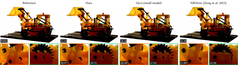
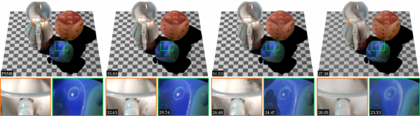
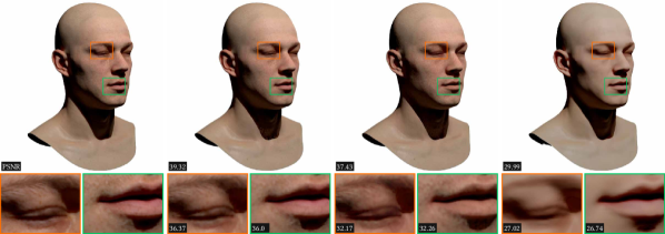
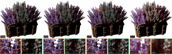
Figure 8. Comparisons with NRHints [Zeng et al., 2023] on surface-based assets. We show a comparison with four mesh-based assets under point light illumination. All of them show effects of long light paths due to subsurface scattering applied to varying degrees. One of the assets is from the NRHints paper (jug and dice, second row). Overall, even our real-time model performs as well or better than Zeng et al. [2023], and our high-quality model is consistently better. NRHints has worse depiction of geometric details (lego and flowers) and high frequency texture/shading details (jug/dice and head).

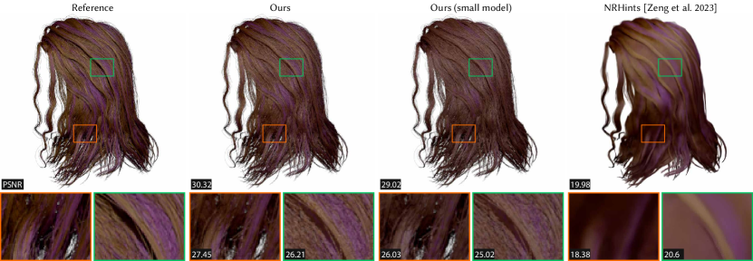
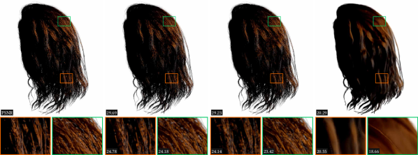
Figure 9. Comparisons with NRHints [Zeng et al., 2023] on fiber-based assets. Fiber-based assets show even more clearly the advantages of our method. Even though [Zeng et al., 2023] learns plausible shading cues and color (for example, the pink highlights in the blonde hair), the results are blurry due to fine geometric details not being reproducible. On the other hand, our results reproduce even the fine structured “glinty” appearance of the fibers, since our method not only uses the ground truth fiber geometry, but also accurately models radiance variation across fiber width. Moreover, the comparison results are rendered under point light illumination to align with the capabilities of the NRHints architecture, which is currently designed to support point lights.

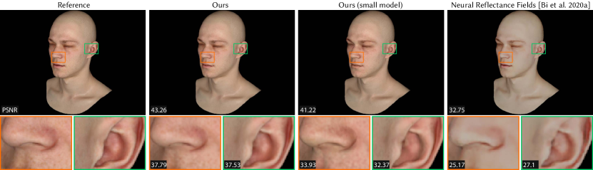
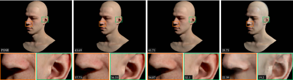
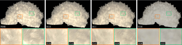
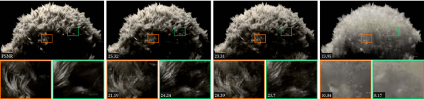
Figure 10. Comparison with Neural Reflectance Fields [Bi et al., 2020], which fits views with collocated point lighting. We compare the methods with both collocated and non-collocated novel point lighting. In both cases, our method (both high-quality and real-time models) clearly outperforms Bi et al. [2020], as their method approximates the shading by estimating the parameters of a simple surface BRDF model (or Kajiya-Kay hair model for fibers). Even with collocated lighting (first and third row), Bi et al. [2020] is not able to recover the same amount of detail and contrast in the shading as our method.

6.3. Comparison to NRHints on fiber assets

In Figure 9, we show a comparison of our method to path traced reference and NRHints [Zeng et al., 2023] on fiber-based assets (hair and fur), where the effects of detailed geometry and multiple-scattered light paths are even more significant than for surface assets. This is reflected in the corresponding PSNR values, but (in our opinion) it is even more true perceptually.

Our asset representation is sufficiently versatile to replicate widely varying fiber effects. For instance, we showcase two hair models, Blonde Hair and Brown Hair, with dramatically different material settings. The Blonde Hair exhibits a much lighter color due to pronounced multiple scattering, while the Brown Hair is characterized by dominant low-order scattering, accompanied by a distinct secondary (transmit-reflect-transmit) highlight, an important effect detailed by Marschner et al. [2003] that our model reproduces without issues.

Even though [Zeng et al., 2023] learns plausible shading cues and color (for example, the pink highlights in the blonde hair), the results are blurry due to fine geometric details not being reproducible. On the other hand, our results reproduce even the fine structured “glinty” appearance of the fibers. Our PSNR values are consistently better than NRHints, even for our small model, which uses a much smaller neural network than NRHints.

Our method not only uses the ground truth fiber geometry, but also accurately models radiance variation across fiber width; we believe ours is the first neural 3D representation that captures fiber shading at this level of accuracy.

6.4. Comparison to Neural Reflectance Fields

In Figure 10, we show a comparison with Neural Reflectance Fields [Bi et al., 2020], which fits views with collocated point lighting. We chose one surface and one fiber based scene, and compare the methods with both collocated and non-collocated novel point lighting. In all cases, our method (both high-quality and small models) clearly outperforms Bi et al. [2020], as their method approximates the shading by estimating the parameters of a simple surface BRDF model (or Kajiya-Kay hair model for the fiber asset). Even with collocated lighting (first and third row), which matches its lighting assumptions, Bi et al. [2020] is not able to recover the same amount of detail and contrast in the shading as our method.

Lake	Office Hallway	City Plaza	Above the Clouds

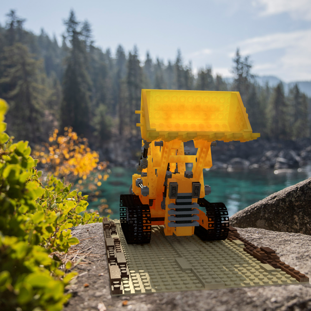
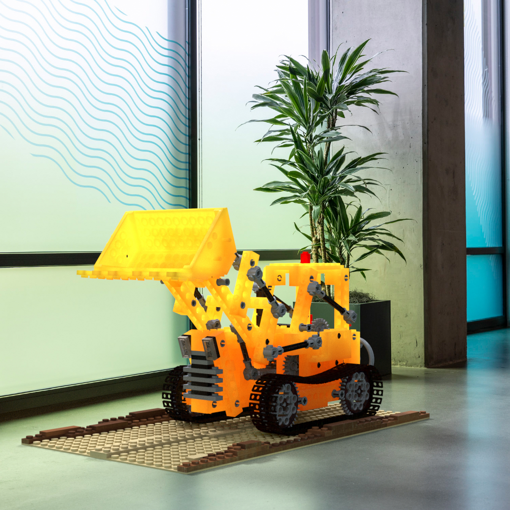
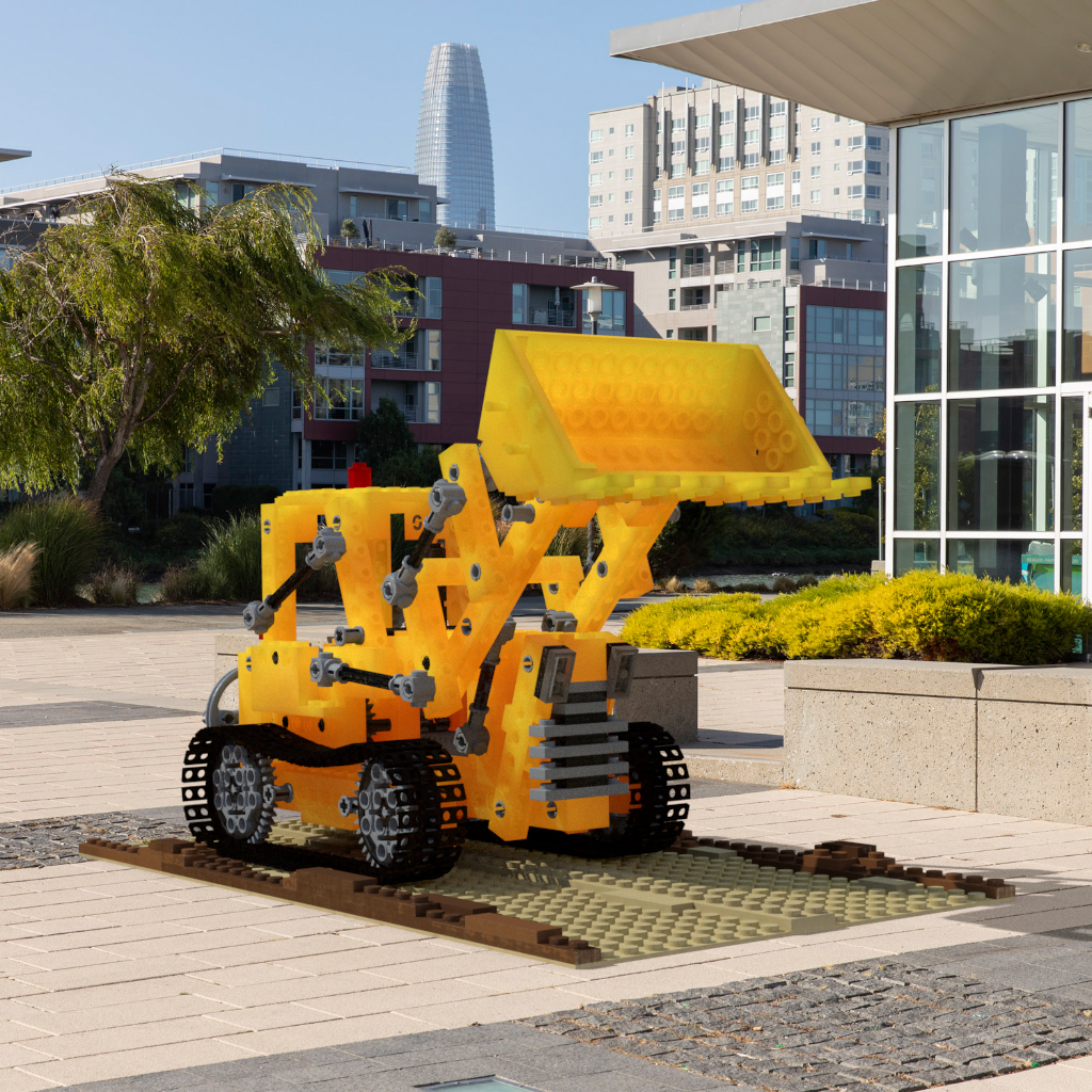
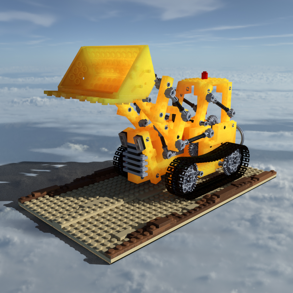
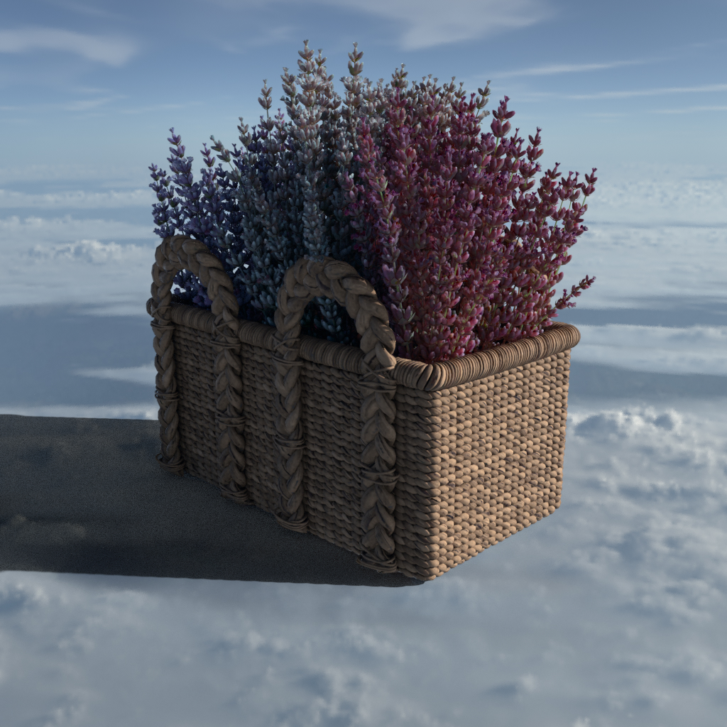
Figure 11. IBL relighting results on surface assets. We render our model under four different IBL environments with shadow-catching ground plane on surface assets, namely the translucent lego and a basket of flowers, both featuring subsurface scattering. The lighting conditions vary from sharp outdoor sunlight to indoor office light, demonstrating our model’s ability to faithfully react to the illuminations for relighting.

Sunset
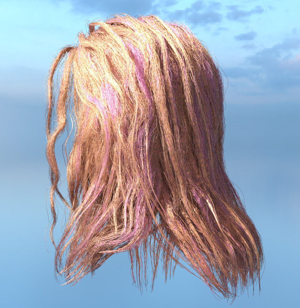
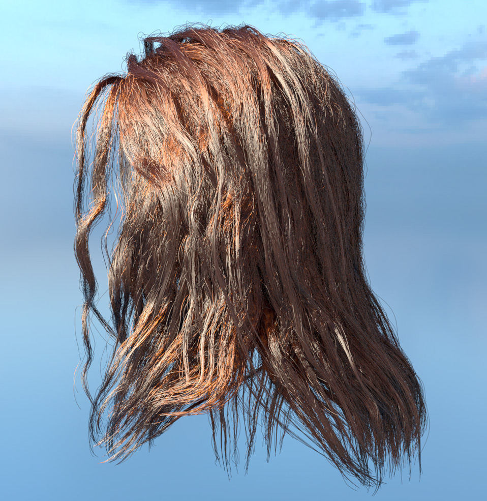
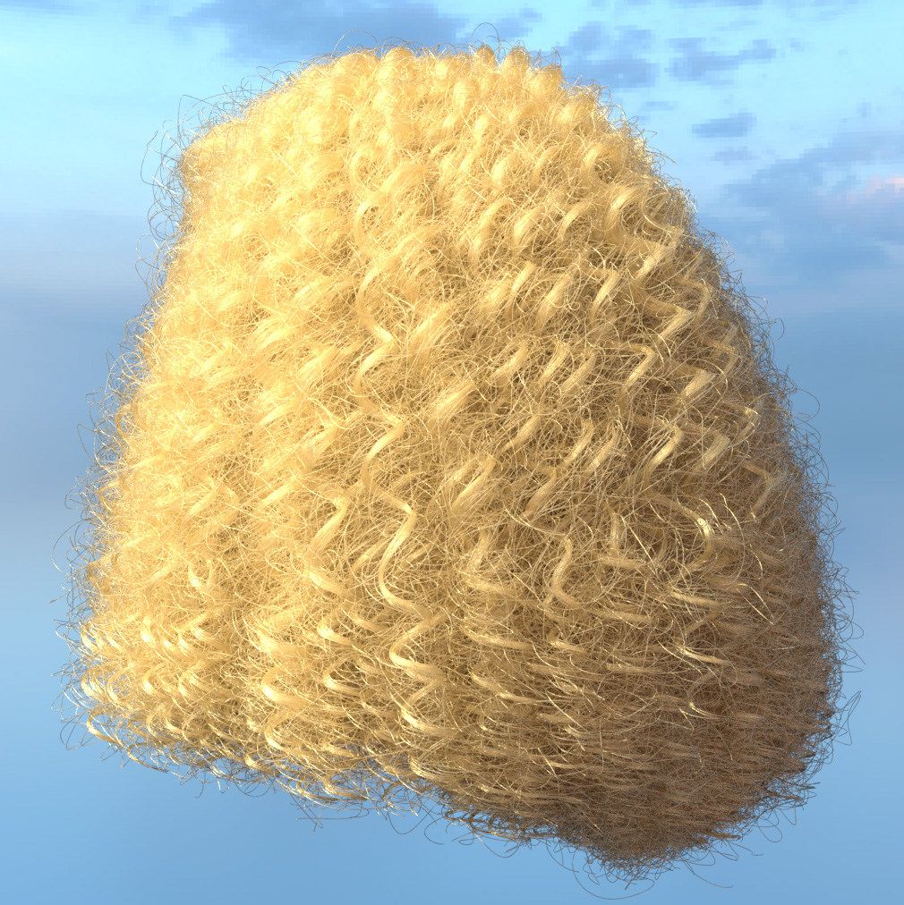
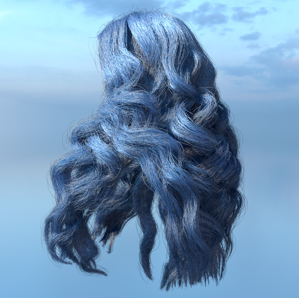
Studio Light

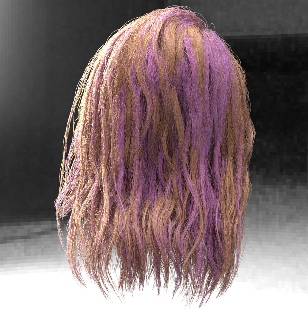
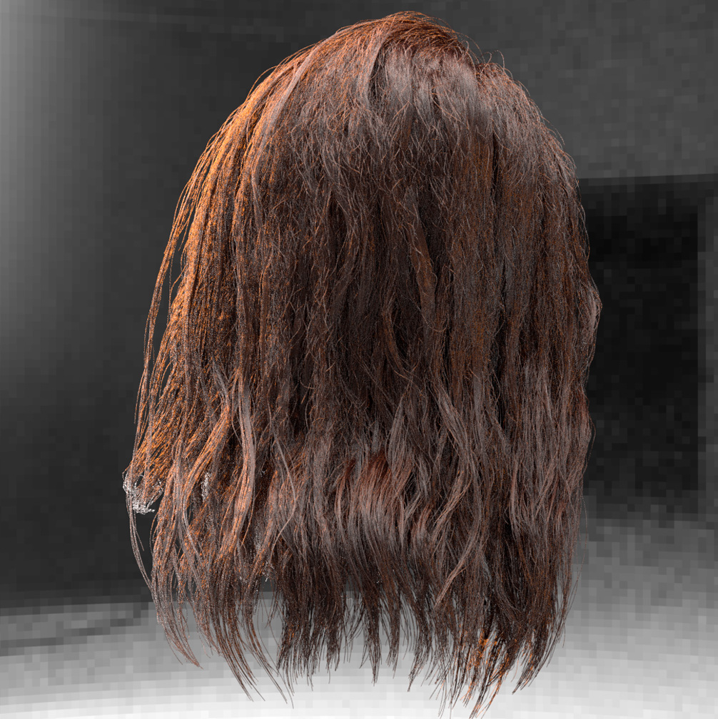
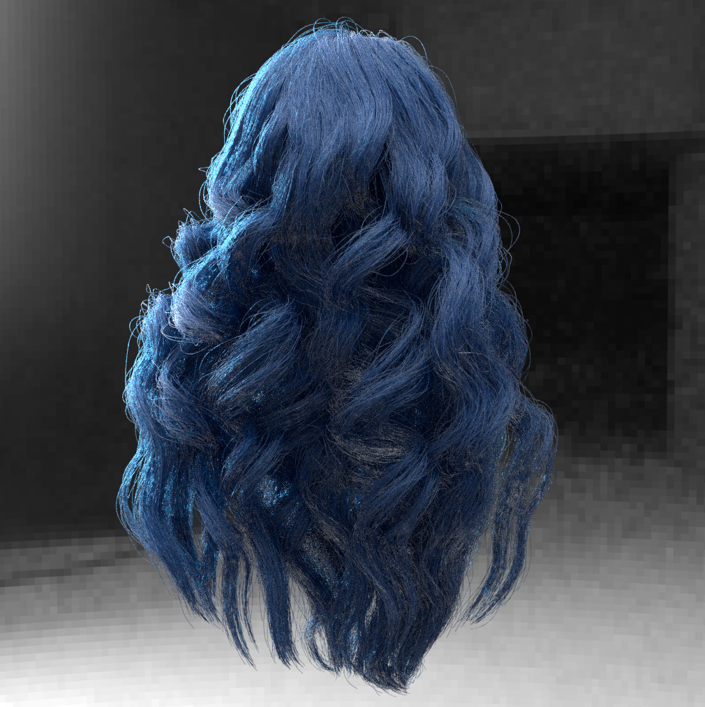
Figure 12. IBL relighting results on fiber assets. Our model is rendered under precise IBL lighting environments, including sunlight and studio light, using four different hair assets with complex scattering effects. It successfully captures the texture of specular glinty highlights and the soft diffusion-like characteristics due to multiple fiber interactions, maintaining the lifelike appearance of individual hair strands and photorealism of the hair appearance, demonstrating reasonable visual accuracy while responding to various illuminations.

6.5. Showcase of our relighting results

In addition, we present our model’s capability to relight surface and fiber assets under varying lighting conditions. As illustrated in Figure 11, we render a translucent Lego and a basket of flowers, both with subsurface scagttering, under four distinct IBL illuminations, each with a shadow-casting ground plane. The selected IBL environments—Lake, Office Hallway, City Plaza, and Above the Clouds—encompass a diverse array of lighting scenarios, both indoor and outdoor. Our relightable neural assets consistently demonstrate the visual transformation of a single asset under varied illuminations but also emphasize the rich detail and photorealism that can be achieved, highlighting the intricate subtleties of light interaction with complex illumination and materials.

In Figure 12, we further demonstrate our model’s relighting capability on fiber assets. Four distinct hair models are each illuminated by an outdoor IBL (Sunset) and an indoor IBL (Studio Light). Our model is capable of accommodating novel perspectives while accurately responding to illumination changes with a complex interplay of highlights, textures, self-shadowing and multiple fiber scattering. We believe no neural rendering methods for full 3D assets have shown comparably powerful relighting ability under arbitrary views.

6.6. Near-field Rendering

As described in Section 3, our model is trained under the assumption of distant lighting. In figure 13, we analyze the effect of this assumption on near-field lighting with the use of a point light placed at three different distances from the neural asset. We observe that on moving the point light from a relatively far distance of $8.66$ closer to $1.73$, our model’s accuracy holds up particularly well as shown by very similar PSNR values in both the full render and crops. Even when the light is moved right next to the asset at a distance of $0.86$, the overall appearance is preserved, but the close-up crops show some reduction in quality. This shows that for most practical applications, the distant light assumption does not cause our method to break down on using local lighting. We would also like to also note that all the comparisons to baselines were performed with point lights showing further evidence of near-field rendering quality.

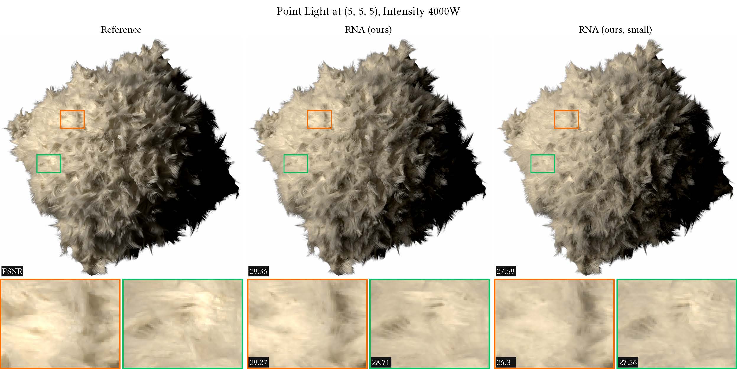
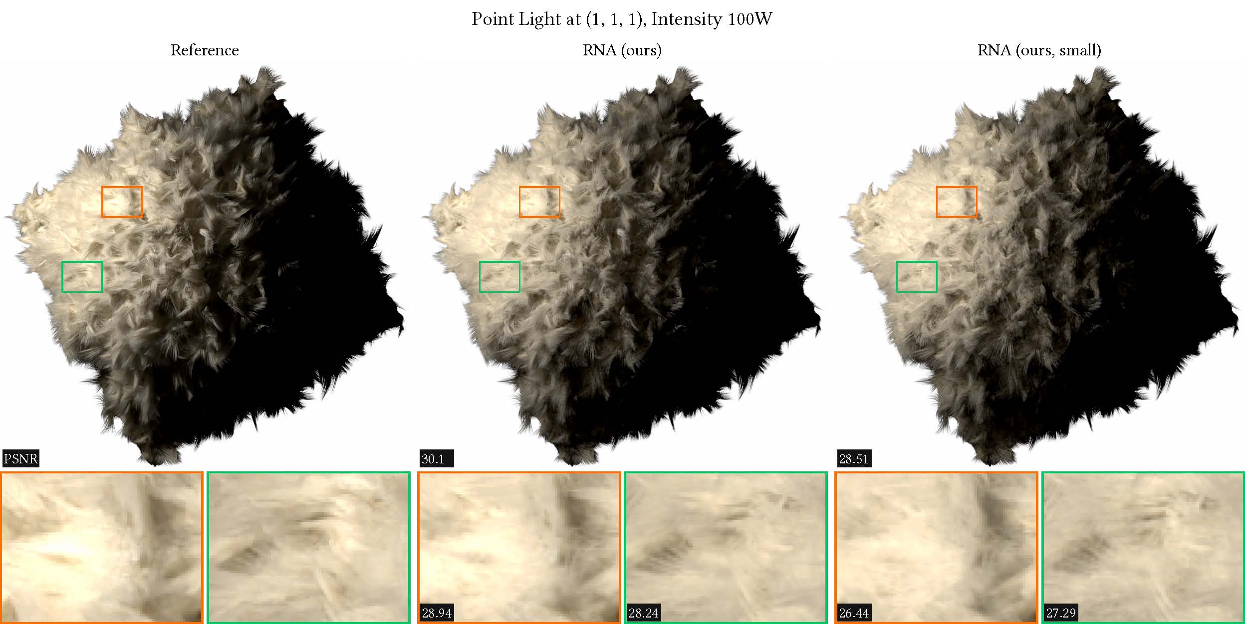
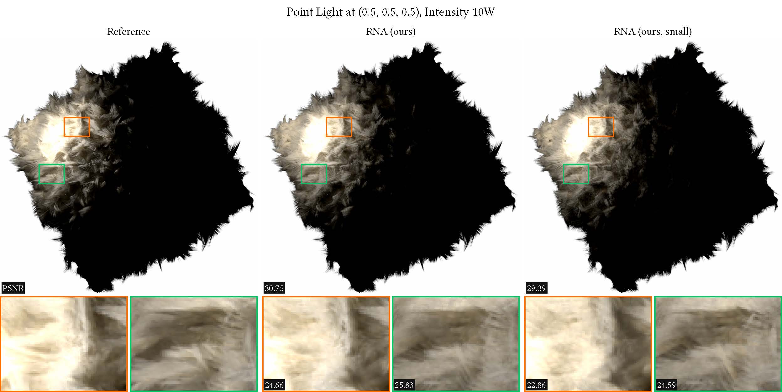
Figure 13. Near-field lighting limitation. We show the rendering of our white fur asset with a point light at distances that are far, close and very close to the asset to illustrate to what extent our distant lighting assumption causes error in near-field lighting.

6.7. Ablations

Ours (w/ $h$)	Ours (w/o $h$)	Reference

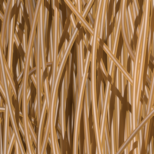
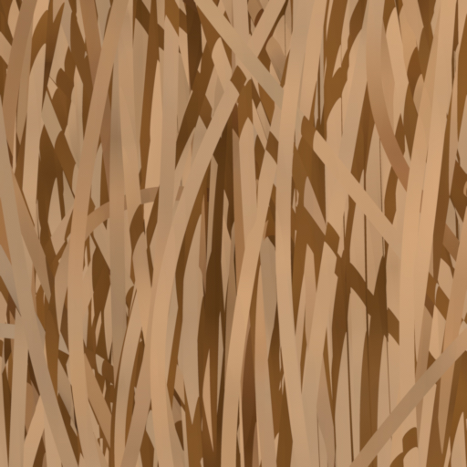
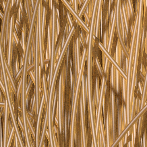
Figure 14. A close-up of a small part of a blonde hair assembly. Our approach can render fairly extreme close-ups that remain detailed and realistic, instead of blurring; however, this requires using the fiber cross-section position $h$ as one of the MLP inputs. Left: without $h$, the model cannot learn the variation. Middle: the variation across the width of a fiber is captured as well as in the reference (right).

6.7.1. Using $h$

In Figure 14, we show a close-up zoom at a small part of a hair assembly. Our model computes point-wise outgoing radiance at every fiber intersection. This lets us render fairly extreme close-ups that remain detailed and realistic, instead of blurring (which would have been the case for volumetric or mesh approximations to the fiber geometry). Note the variation in color across the width of a fiber (middle), a correctly captured feature of the near-field hair BSDF model used, matching the reference (right). However, this requires using the fiber cross-section position $h$ as one of the MLP inputs. Without $h$, the model cannot learn the variation (left).

6.7.2. Network Architecture

We chose MLP and triplane configurations methodically. Table 1 shows the various MLP architectures we tested, along with their training time and average PSNR values on the validation data for the Lego asset that has heavy scattering properties in its shading model. It is clear that increasing the network capacity improved the quality of the model, and took longer to train; the training time being a rough estimate of the model’s inference performance. Of note, for the Lego asset, models with 16 and 32 hidden layer neurons were not able to capture the scattering effects in most regions and 64 was the fastest acceptable one. We chose 64 neurons as the size for the small model as it worked well with all our assets, and was also a size that generally fits on register allocations of GPU production path tracing shaders. The take-away though is that there is a quality vs. performance trade-off that can be made for any particular use case.

Table 2 shows the effect of using feature grids with increasing channel counts on our high-quality model. Increasing the number of channels increases the number of inputs to the MLP and thus has an adverse effect on performance as indicated by training time. The PSNR values show that 8 channels is sufficient for good model quality, and though there is a slight benefit in going up to 16 channels, anything higher doesn’t provide additional gains.

Table 1. Ablation on the MLP architecture. We evaluate different configurations of the MLP, including the number of hidden layers and the number of neurons in each layer. We show the average PSNRs on the Lego asset, along with the runtime for training to give a sense of model performance. All models here use 8 channels for the feature grids. Our chosen architecture for offline model is in bold, and small model is in italics.

Hidden Layers	Neurons	Training Runtime	PSNR
4	16	34m 58s	27.47
4	32	35m 11s	27.36
4	64	31m 17s	28.77
4	128	39m 27s	31.02
4	256	50m 51s	32.68
2	512	55m 51s	33.07
3	512	1h 5m	33.80
4	512	1h 13m	34.09
5	512	1h 25m	34.20
4	1024	2h 44m	34.90

Table 2. Ablation on Feature Grid Channels. We evaluate use of different feature grid channels on the Lego asset with our high-quality model that has 4 hidden layers with 512 neurons each.

Channels	Training Runtime	PSNR
4	1h 11m	33.51
8	1h 13m	34.09
16	1h 20m	34.40
32	1h 37m	34.33

6.7.3. Visibility

We compare the rendering result of our model with and without the lighting visibility hint. As shown in Figure 15, our model improves the rendering quality around shadowing edges with faithful shadows when we provide visibility hints to the MLP. This is because direct shadowing is typically high frequency signals (e.g. hard edge boundaries), which is difficult for MLP to represent well without aiding such hints.

Ours (w/ vis. hint)	Vis. hint	Ours (w/o vis. hint)

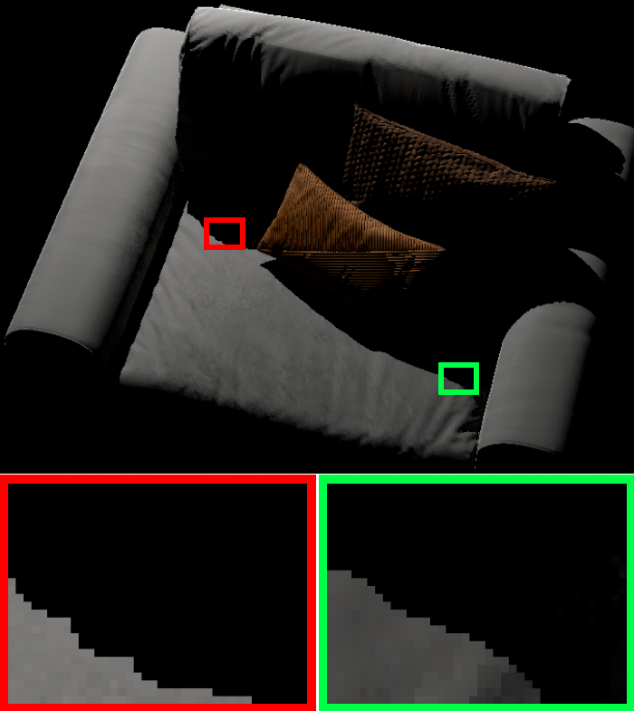
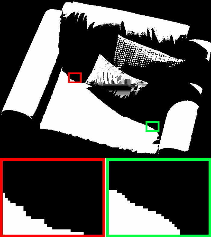
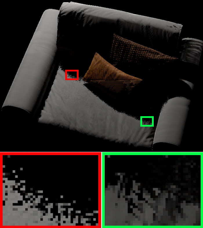
Figure 15. Lighting visibility for self-shadowing. We use visibility value as a hint to the MLP, which significantly improves the rendering quality around shadowing edges.

6.7.4. Triplane vs. UV parameterization

As shown in Figure 16, triplane representation provides sufficient texture details at $512\times 512$. On the other hand, UV parameterization at $512\times 512$ resolution results in blurred details, becoming sharper only at $1024\times 1024$. On the other hand, UV mapping is not always feasible when the mesh topology is complex (or fibers) while triplane representation does not have such limitation.

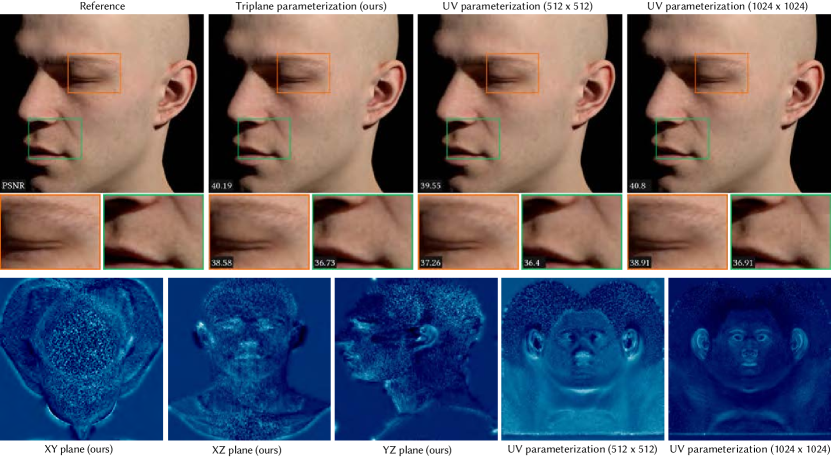
Figure 16. Ablation on the triplane vs. UV parameterization. We examine triplane and UV parameterization on the head asset. UV parameterization at $512\times 512$ resolution results in blurred details, becoming sharper only at $1024\times 1024$. Conversely, the triplane representation provides satisfactory detail at $512\times 512$. The color map is the same as in Fig. 3, visualizing the first channel of features.

6.8. Discussion and limitations

In summary, these results affirm our model’s robustness in managing diverse lighting conditions and viewpoints, as well as its precision in modeling an array of surface types and complex light transport phenomena. We believe our approach has broad applicability, combined with its high performance, positions is as potentially broadly applicable in practice.

Several limitations exist and we would like to address them in future work. One limitation of our current path-tracer integration is that we use simple uniform sampling as an approximation, similar to NeuMIP [Kuznetsov et al., 2021]. A more advanced importance sampling module could be trained, similar to Xu et al. [2023] or Zeltner et al. [2023]. These approaches would require a new sampling neural network, but could reuse the same feature grid from our method.

Furthermore, while our method supports specular objects (e.g. the skin material is fairly specular), very low roughness (close to mirror or glass) materials will show blurring in our fits. Our assets are currently static; animated assets would be an interesting future challenge, and could be supported through mapping shading queries into a canonical pose and training over different poses ins addition to camera and light directions. Furthermore, while primary ray-tracing of the explicit geometry is cheaper than full light transport, it may still be expensive for some applications; this could be addressed by an approximate proxy geometry.

7. Conclusion

In this paper, we introduced a precomputed relightable neural model for representing synthetic surface-based or fiber-based 3D assets with complex materials. Our model allows full view and lighting variation; in comparison with relightable neural capture approaches, we achieve higher accuracy, though our method is specifically designed for representing digital assets, not for capture from real photographs. Our design enables any viewing or illumination conditions and allows for integration of our assets in full scenes, rendered in a production path tracer. Our neural model handles all shading, inter-reflections, and scattering. The benefits of our approach include increased shading performance, as well as as ability to represent complex material models and shading graphs, which do not need to be implemented in the target rendering system.

References

- [1]
- Bangaru et al. [2022] Sai Praveen Bangaru, Michaël Gharbi, Tzu-Mao Li, Fujun Luan, Kalyan Sunkavalli, Milos Hasan, Sai Bi, Zexiang Xu, Gilbert Bernstein, and Fredo Durand. 2022. Differentiable rendering of neural sdfs through reparameterization. In SIGGRAPH Asia 2022 Conference Papers. 1–9.
- Belcour [2018] Laurent Belcour. 2018. Efficient rendering of layered materials using an atomic decomposition with statistical operators. ACM Transactions on Graphics 37, 4 (2018), 1.
- Ben-Artzi et al. [2008] Aner Ben-Artzi, Kevin Egan, Frédo Durand, and Ravi Ramamoorthi. 2008. A Precomputed Polynomial Representation for Interactive BRDF Editing with Global Illumination. ACM Trans. Graph. 27, 2, Article 13 (may 2008), 13 pages. https://doi.org/10.1145/1356682.1356686
- Bi et al. [2020] Sai Bi, Zexiang Xu, Pratul P. Srinivasan, Ben Mildenhall, Kalyan Sunkavalli, Milos Hasan, Yannick Hold-Geoffroy, David J. Kriegman, and Ravi Ramamoorthi. 2020. Neural Reflectance Fields for Appearance Acquisition. abs/2008.03824 (2020). arXiv:2008.03824 https://arxiv.org/abs/2008.03824
- Boss et al. [2021a] Mark Boss, Raphael Braun, Varun Jampani, Jonathan T Barron, Ce Liu, and Hendrik Lensch. 2021a. Nerd: Neural reflectance decomposition from image collections. In Proceedings of the IEEE/CVF International Conference on Computer Vision. 12684–12694.
- Boss et al. [2021b] Mark Boss, Varun Jampani, Raphael Braun, Ce Liu, Jonathan Barron, and Hendrik Lensch. 2021b. Neural-pil: Neural pre-integrated lighting for reflectance decomposition. Advances in Neural Information Processing Systems 34 (2021), 10691–10704.
- Cai et al. [2022] Guangyan Cai, Kai Yan, Zhao Dong, Ioannis Gkioulekas, and Shuang Zhao. 2022. Physics-based inverse rendering using combined implicit and explicit geometries. In Computer Graphics Forum, Vol. 41. Wiley Online Library, 129–138.
- Chan et al. [2022] Eric R Chan, Connor Z Lin, Matthew A Chan, Koki Nagano, Boxiao Pan, Shalini De Mello, Orazio Gallo, Leonidas J Guibas, Jonathan Tremblay, Sameh Khamis, et al. 2022. Efficient geometry-aware 3D generative adversarial networks. In Proceedings of the IEEE/CVF Conference on Computer Vision and Pattern Recognition. 16123–16133.
- Chan et al. [2021] Eric R. Chan, Connor Z. Lin, Matthew A. Chan, Koki Nagano, Boxiao Pan, Shalini De Mello, Orazio Gallo, Leonidas Guibas, Jonathan Tremblay, Sameh Khamis, Tero Karras, and Gordon Wetzstein. 2021. Efficient Geometry-aware 3D Generative Adversarial Networks. In arXiv.
- Chen et al. [2022] Anpei Chen, Zexiang Xu, Andreas Geiger, Jingyi Yu, and Hao Su. 2022. TensoRF: Tensorial Radiance Fields. arXiv preprint arXiv:2203.09517 (2022).
- Chiang et al. [2016] Matt Jen-Yuan Chiang, Benedikt Bitterli, Chuck Tappan, and Brent Burley. 2016. A Practical and Controllable Hair and Fur Model for Production Path Tracing. Computer Graphics Forum (2016). https://doi.org/10.1111/cgf.12830
- Christensen [2015] Per H Christensen. 2015. An approximate reflectance profile for efficient subsurface scattering. In ACM SIGGRAPH 2015 Talks. 1–1.
- Chu and Thuerey [2017] Mengyu Chu and Nils Thuerey. 2017. Data-driven synthesis of smoke flows with CNN-based feature descriptors. ACM Transactions on Graphics (TOG) 36, 4 (2017), 1–14.
- Dana et al. [1999] Kristin J. Dana, Bram van Ginneken, Shree K. Nayar, and Jan J. Koenderink. 1999. Reflectance and Texture of Real-World Surfaces. ACM Trans. Graph. 18, 1 (jan 1999), 1–34. https://doi.org/10.1145/300776.300778
- d’Eon et al. [2011] Eugene d’Eon, Guillaume Francois, Martin Hill, Joe Letteri, and Jean-Marie Aubry. 2011. An energy-conserving hair reflectance model. In Computer Graphics Forum, Vol. 30. Wiley Online Library, 1181–1187.
- Donner and Jensen [2006] Craig Donner and Henrik Wann Jensen. 2006. A Spectral BSSRDF for Shading Human Skin. Rendering techniques 2006 (2006), 409–418.
- Donner et al. [2008] Craig Donner, Tim Weyrich, Eugene d’Eon, Ravi Ramamoorthi, and Szymon Rusinkiewicz. 2008. A layered, heterogeneous reflectance model for acquiring and rendering human skin. ACM transactions on graphics (TOG) 27, 5 (2008), 1–12.
- Gao et al. [2020] Duan Gao, Guojun Chen, Yue Dong, Pieter Peers, Kun Xu, and Xin Tong. 2020. Deferred neural lighting: free-viewpoint relighting from unstructured photographs. ACM Transactions on Graphics (TOG) 39, 6 (2020), 1–15.
- Guo et al. [2016] Jie Guo, Jinghui Qian, Yanwen Guo, and Jingui Pan. 2016. Rendering thin transparent layers with extended normal distribution functions. IEEE transactions on visualization and computer graphics 23, 9 (2016), 2108–2119.
- Guo et al. [2018] Yu Guo, Miloš Hašan, and Shuang Zhao. 2018. Position-free Monte Carlo simulation for arbitrary layered BSDFs. ACM Transactions on Graphics (ToG) 37, 6 (2018), 1–14.
- Habel et al. [2013] Ralf Habel, Per H Christensen, and Wojciech Jarosz. 2013. Photon beam diffusion: A hybrid monte carlo method for subsurface scattering. In Computer Graphics Forum, Vol. 32. Wiley Online Library, 27–37.
- Hasselgren et al. [2022] Jon Hasselgren, Nikolai Hofmann, and Jacob Munkberg. 2022. Shape, light, and material decomposition from images using Monte Carlo rendering and denoising. Advances in Neural Information Processing Systems 35 (2022), 22856–22869.
- Jensen et al. [2001] Henrik Wann Jensen, Stephen R Marschner, Marc Levoy, and Pat Hanrahan. 2001. A practical model for subsurface light transport. In Proceedings of the 28th annual conference on Computer graphics and interactive techniques. 511–518.
- Jin et al. [2023] Haian Jin, Isabella Liu, Peijia Xu, Xiaoshuai Zhang, Songfang Han, Sai Bi, Xiaowei Zhou, Zexiang Xu, and Hao Su. 2023. TensoIR: Tensorial Inverse Rendering. arXiv:2304.12461
- Kallweit et al. [2017] Simon Kallweit, Thomas Müller, Brian Mcwilliams, Markus Gross, and Jan Novák. 2017. Deep scattering: Rendering atmospheric clouds with radiance-predicting neural networks. ACM Transactions on Graphics (TOG) 36, 6 (2017), 1–11.
- Khungurn and Marschner [2017] Pramook Khungurn and Steve Marschner. 2017. Azimuthal scattering from elliptical hair fibers. ACM Transactions on Graphics (TOG) 36, 2 (2017), 1–23.
- Kingma and Ba [2014] Diederik P Kingma and Jimmy Ba. 2014. Adam: A method for stochastic optimization. arXiv preprint arXiv:1412.6980 (2014).
- Kuang et al. [2022] Zhengfei Kuang, Kyle Olszewski, Menglei Chai, Zeng Huang, Panos Achlioptas, and Sergey Tulyakov. 2022. Neroic: Neural rendering of objects from online image collections. ACM Transactions on Graphics (TOG) 41, 4 (2022), 1–12.
- Kuznetsov et al. [2021] Alexandr Kuznetsov, Krishna Mullia, Zexiang Xu, Miloš Hašan, and Ravi Ramamoorthi. 2021. NeuMIP: Multi-Resolution Neural Materials. Transactions on Graphics (Proceedings of SIGGRAPH) 40, 4, Article 175 (July 2021), 13 pages.
- Kuznetsov et al. [2022] Alexandr Kuznetsov, Xuezheng Wang, Krishna Mullia, Fujun Luan, Zexiang Xu, Miloš Hašan, and Ravi Ramamoorthi. 2022. Rendering Neural Materials on Curved Surfaces. In ACM SIGGRAPH 2022 Conference Proceedings. 1–9.
- Luan et al. [2021] Fujun Luan, Shuang Zhao, Kavita Bala, and Zhao Dong. 2021. Unified shape and svbrdf recovery using differentiable monte carlo rendering. In Computer Graphics Forum, Vol. 40. Wiley Online Library, 101–113.
- Mao et al. [2023] Shi Mao, Chenming Wu, Zhelun Shen, and Liangjun Zhang. 2023. NeuS-PIR: Learning Relightable Neural Surface using Pre-Integrated Rendering. arXiv preprint arXiv:2306.07632 (2023).
- Marschner et al. [2003] Stephen R Marschner, Henrik Wann Jensen, Mike Cammarano, Steve Worley, and Pat Hanrahan. 2003. Light scattering from human hair fibers. ACM Transactions on Graphics (TOG) 22, 3 (2003), 780–791.
- Mildenhall et al. [2020] Ben Mildenhall, Pratul P. Srinivasan, Matthew Tancik, Jonathan T. Barron, Ravi Ramamoorthi, and Ren Ng. 2020. NeRF: Representing Scenes as Neural Radiance Fields for View Synthesis. In ECCV.
- Mildenhall et al. [2021] Ben Mildenhall, Pratul P Srinivasan, Matthew Tancik, Jonathan T Barron, Ravi Ramamoorthi, and Ren Ng. 2021. Nerf: Representing scenes as neural radiance fields for view synthesis. Commun. ACM 65, 1 (2021), 99–106.
- Müller et al. [2022] Thomas Müller, Alex Evans, Christoph Schied, and Alexander Keller. 2022. Instant neural graphics primitives with a multiresolution hash encoding. arXiv preprint arXiv:2201.05989 (2022).
- Munkberg et al. [2022] Jacob Munkberg, Jon Hasselgren, Tianchang Shen, Jun Gao, Wenzheng Chen, Alex Evans, Thomas Müller, and Sanja Fidler. 2022. Extracting triangular 3d models, materials, and lighting from images. In Proceedings of the IEEE/CVF Conference on Computer Vision and Pattern Recognition. 8280–8290.
- Ng et al. [2003] Ren Ng, Ravi Ramamoorthi, and Pat Hanrahan. 2003. All-Frequency Shadows Using Non-Linear Wavelet Lighting Approximation. ACM Trans. Graph. 22, 3 (jul 2003), 376–381. https://doi.org/10.1145/882262.882280
- Ng et al. [2004] Ren Ng, Ravi Ramamoorthi, and Pat Hanrahan. 2004. Triple Product Wavelet Integrals for All-Frequency Relighting. ACM Trans. Graph. 23, 3 (aug 2004), 477–487. https://doi.org/10.1145/1015706.1015749
- Rainer et al. [2019] Gilles Rainer, Wenzel Jakob, Abhijeet Ghosh, and Tim Weyrich. 2019. Neural BTF Compression and Interpolation. Computer Graphics Forum (Proceedings of Eurographics) 38, 2 (March 2019).
- Ramamoorthi [2009] Ravi Ramamoorthi. 2009. Precomputation-Based Rendering. NOW Publishers Inc. http://graphics.cs.berkeley.edu/papers/Ramamoorthi-PBR-2009-04/
- Ren et al. [2015] Peiran Ren, Yue Dong, Stephen Lin, Xin Tong, and Baining Guo. 2015. Image based relighting using neural networks. ACM Transactions on Graphics (ToG) 34, 4 (2015), 1–12.
- Ren et al. [2013] Peiran Ren, Jiaping Wang, Minmin Gong, Stephen Lin, Xin Tong, and Baining Guo. 2013. Global illumination with radiance regression functions. ACM Trans. Graph. 32, 4 (2013), 130–1.
- Sloan et al. [2002] Peter-Pike Sloan, Jan Kautz, and John Snyder. 2002. Precomputed Radiance Transfer for Real-Time Rendering in Dynamic, Low-Frequency Lighting Environments. ACM Trans. Graph. 21, 3 (jul 2002), 527–536. https://doi.org/10.1145/566654.566612
- Srinivasan et al. [2021] Pratul P Srinivasan, Boyang Deng, Xiuming Zhang, Matthew Tancik, Ben Mildenhall, and Jonathan T Barron. 2021. Nerv: Neural reflectance and visibility fields for relighting and view synthesis. In Proceedings of the IEEE/CVF Conference on Computer Vision and Pattern Recognition. 7495–7504.
- Sun et al. [2023a] Cheng Sun, Guangyan Cai, Zhengqin Li, Kai Yan, Cheng Zhang, Carl Marshall, Jia-Bin Huang, Shuang Zhao, and Zhao Dong. 2023a. Neural-PBIR Reconstruction of Shape, Material, and Illumination. arXiv:2304.13445 [cs.CV]
- Sun et al. [2023b] Cheng Sun, Guangyan Cai, Zhengqin Li, Kai Yan, Cheng Zhang, Carl Marshall, Jia-Bin Huang, Shuang Zhao, and Zhao Dong. 2023b. Neural-PBIR Reconstruction of Shape, Material, and Illumination. In Proceedings of the IEEE/CVF International Conference on Computer Vision. 18046–18056.
- Tsai and Shih [2006] Yu-Ting Tsai and Zen-Chung Shih. 2006. All-frequency precomputed radiance transfer using spherical radial basis functions and clustered tensor approximation. ACM Transactions on graphics (TOG) 25, 3 (2006), 967–976.
- Vicini et al. [2019] Delio Vicini, Vladlen Koltun, and Wenzel Jakob. 2019. A learned shape-adaptive subsurface scattering model. ACM Transactions on Graphics (TOG) 38, 4 (2019), 1–15.
- Wrenninge et al. [2017] Magnus Wrenninge, Ryusuke Villemin, and Christophe Hery. 2017. Path traced subsurface scattering using anisotropic phase functions and non-exponential free flights. In Tech. Rep. Pixar Inc.
- Wu et al. [2023] Haoqian Wu, Zhipeng Hu, Lincheng Li, Yongqiang Zhang, Changjie Fan, and Xin Yu. 2023. NeFII: Inverse Rendering for Reflectance Decomposition with Near-Field Indirect Illumination. In Proceedings of the IEEE/CVF Conference on Computer Vision and Pattern Recognition. 4295–4304.
- Xu et al. [2023] Bing Xu, Liwen Wu, Milos Hasan, Fujun Luan, Iliyan Georgiev, Zexiang Xu, and Ravi Ramamoorthi. 2023. NeuSample: Importance Sampling for Neural Materials. In ACM SIGGRAPH 2023 Conference Proceedings (SIGGRAPH ’23). Article 41, 10 pages.
- Xu et al. [2013] Kun Xu, Wei-Lun Sun, Zhao Dong, Dan-Yong Zhao, Run-Dong Wu, and Shi-Min Hu. 2013. Anisotropic spherical gaussians. ACM Transactions on Graphics (TOG) 32, 6 (2013), 1–11.
- Xu et al. [2022] Zilin Xu, Zheng Zeng, Lifan Wu, Lu Wang, and Ling-Qi Yan. 2022. Lightweight Neural Basis Functions for All-Frequency Shading. In SIGGRAPH Asia 2022 Conference Papers. 1–9.
- Yan et al. [2015] Ling-Qi Yan, Chi-Wei Tseng, Henrik Wann Jensen, and Ravi Ramamoorthi. 2015. Physically-accurate fur reflectance: Modeling, measurement and rendering. ACM Transactions on Graphics (TOG) 34, 6 (2015), 1–13.
- Yao et al. [2022] Yao Yao, Jingyang Zhang, Jingbo Liu, Yihang Qu, Tian Fang, David McKinnon, Yanghai Tsin, and Long Quan. 2022. Neilf: Neural incident light field for physically-based material estimation. In European Conference on Computer Vision. Springer, 700–716.
- Yu et al. [2021] Alex Yu, Sara Fridovich-Keil, Matthew Tancik, Qinhong Chen, Benjamin Recht, and Angjoo Kanazawa. 2021. Plenoxels: Radiance fields without neural networks. arXiv preprint arXiv:2112.05131 (2021).
- Zeltner et al. [2023] Tizian Zeltner, Fabrice Rousselle, Andrea Weidlich, Petrik Clarberg, Jan Novák, Benedikt Bitterli, Alex Evans, Tomáš Davidovič, Simon Kallweit, and Aaron Lefohn. 2023. Real-Time Neural Appearance Models. arXiv preprint arXiv:2305.02678 (2023).
- Zeng et al. [2023] Chong Zeng, Guojun Chen, Yue Dong, Pieter Peers, Hongzhi Wu, and Xin Tong. 2023. Relighting Neural Radiance Fields with Shadow and Highlight Hints. In ACM SIGGRAPH 2023 Conference Proceedings. 1–11.
- Zhang et al. [2022a] Kai Zhang, Fujun Luan, Zhengqi Li, and Noah Snavely. 2022a. Iron: Inverse rendering by optimizing neural sdfs and materials from photometric images. In Proceedings of the IEEE/CVF Conference on Computer Vision and Pattern Recognition. 5565–5574.
- Zhang et al. [2021a] Kai Zhang, Fujun Luan, Qianqian Wang, Kavita Bala, and Noah Snavely. 2021a. Physg: Inverse rendering with spherical gaussians for physics-based material editing and relighting. In Proceedings of the IEEE/CVF Conference on Computer Vision and Pattern Recognition. 5453–5462.
- Zhang et al. [2021b] Xiuming Zhang, Pratul P Srinivasan, Boyang Deng, Paul Debevec, William T Freeman, and Jonathan T Barron. 2021b. Nerfactor: Neural factorization of shape and reflectance under an unknown illumination. ACM Transactions on Graphics (ToG) 40, 6 (2021), 1–18.
- Zhang et al. [2022b] Yuanqing Zhang, Jiaming Sun, Xingyi He, Huan Fu, Rongfei Jia, and Xiaowei Zhou. 2022b. Modeling indirect illumination for inverse rendering. In Proceedings of the IEEE/CVF Conference on Computer Vision and Pattern Recognition. 18643–18652.
- Zhang et al. [2023] Youjia Zhang, Teng Xu, Junqing Yu, Yuteng Ye, Yanqing Jing, Junle Wang, Jingyi Yu, and Wei Yang. 2023. Nemf: Inverse volume rendering with neural microflake field. In Proceedings of the IEEE/CVF International Conference on Computer Vision. 22919–22929.
- Zhu et al. [2021] Junqiu Zhu, Yaoyi Bai, Zilin Xu, Steve Bako, Edgar Velázquez-Armendáriz, Lu Wang, Pradeep Sen, Miloš Hašan, and Ling-Qi Yan. 2021. Neural complex luminaires: representation and rendering. ACM Transactions on Graphics (TOG) 40, 4 (2021), 1–12.
- Zinke et al. [2008] Arno Zinke, Cem Yuksel, Andreas Weber, and John Keyser. 2008. Dual scattering approximation for fast multiple scattering in hair. In ACM SIGGRAPH 2008 papers. 1–10.