HiER: Highlight Experience Replay and Easy2Hard Curriculum Learning for Boosting Off-Policy Reinforcement Learning Agents

Abstract

Even though reinforcement-learning-based algorithms achieved superhuman performance in many domains, the field of robotics poses significant challenges as the state and action spaces are continuous, and the reward function is predominantly sparse. In this work, we propose: 1) HiER: highlight experience replay that creates a secondary replay buffer for the most relevant experiences, 2) E2H-ISE: an easy2hard data collection curriculum-learning method based on controlling the entropy of the initial state-goal distribution and with it, indirectly, the task difficulty, and 3) HiER+: the combination of HiER and E2H-ISE. They can be applied with or without the techniques of hindsight experience replay (HER) and prioritized experience replay (PER). While both HiER and E2H-ISE surpass the baselines, HiER+ further improves the results and significantly outperforms the state-of-the-art on the push, slide, and pick-and-place robotic manipulation tasks. Our implementation and further media materials are available on the project site.

I INTRODUCTION

A high degree of transferability is essential to create universal robotic solutions. While transferring knowledge between domains [1, 2, 3], robotic systems [4], or tasks [5] is fundamental, it is essential to create and apply universal methods such as reinforcement-learning-based algorithms (RL) [6, 7, 8, 9] which are inspired by the profoundly universal trial-and-error-based human/animal learning.

RL methods, especially combined with neural networks (deep reinforcement learning), were proven to be superior in many fields such as achieving superhuman performance in chess [10], Go [11], or Atari games [12]. Nevertheless, in the field of robotics, there are significant challenges yet to overcome. Most importantly, the state and action spaces are continuous which intensifies the challenge of exploration. Oftentimes, discretization is not feasible due to loss of information or accuracy, preventing the application of tabular RL methods with high stability. Furthermore, the reward functions of robotic tasks are predominantly sparse which escalates the difficulty of exploration.

Introducing prior knowledge in the form of reward shaping could facilitate the exploration by guiding the agent towards the desired solution. However, 1) constructing a sophisticated reward function requires expert knowledge, 2) the reward function is task-specific, and 3) the agent might learn undesired behaviors. Another source of prior knowledge could be in the form of expert demonstrations. However, collecting demonstrations is oftentimes expensive (time and resources) or even not feasible. Furthermore, it constrains transferability as demonstrations are task-specific.

In parallel to constructing more efficient RL algorithms such as state-of-the-art actor-critic models (DDPG [6, 7], TD3 [8], and SAC [9]), another line of research focuses on improving existing RL algorithms by controlling the data collection [13, 14, 15, 16, 17, 18, 19, 20, 21] or the data exploitation [22, 23, 24, 25, 26, 27]. The latter direction of research belongs to the field of curriculum learning (CL) [28, 29, 30].

Our target is to facilitate the training of off-policy RL agents with our CL methods. Our contributions are the following:

1. HiER: The technique of highlight experience replay is a data exploitation CL method. It creates a secondary experience replay buffer to store the most relevant transitions. It can be added to any off-policy RL agent. If only positive experiences are stored in its buffer, HiER can be viewed as a special, automatic demonstration generator as well.

2. E2H-ISE: An easy2hard data collection CL method that controls the entropy of the initial state-goal distribution $\mathcal{H}(\mu_{0})$ which indirectly controls the task difficulty. ISE stands for initial state entropy.

3. HiER+: The combination of HiER and E2H-ISE. In theory, instead of E2H-ISE, other data collection CL methods could be utilized in HiER+. The overview of HiER+ is depicted in Fig.1.

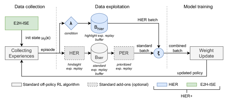
Figure 1: The overview of HiER+. For every episode, the initial state is sampled from $\mu_{0}$ controlled by E2H-ISE. After every episode, the transitions are stored in $\mathcal{B}_{ser}$, and in case the $\lambda$ condition is fulfilled then in $\mathcal{B}_{hier}$ as well. For training, the transitions are sampled from both $\mathcal{B}_{ser}$ and $\mathcal{B}_{hier}$ according to the ratio $\xi$. For detailed description, see Alg. 1.

While both HiER and E2H-ISE surpass the baselines, HiER+ further improves the results and significantly outperforms the state-of-the-art on the push, slide, and pick-and-place robotic manipulation tasks.

The paper is structured as follows: in Section II and III, the essentials of RL and CL are described followed by a literature review. In Section IV and V, HiER, E2H-ISE, and HiER+ are presented with the experimental results. Finally, the summary of our findings is provided in Section VI.

II Background

II-A Reinforcement Learning

In reinforcement learning, an agent attempts to learn the optimal policy for a task through interactions with an environment. It can be formalized with a Markov decision process represented by the state space $\mathcal{S}$, the action space $\mathcal{A}$, the transition probability $p(s_{t+1}|s_{t},a_{t})$, where $s\in\mathcal{S}$ and $a\in\mathcal{A}$, the reward function $r:\mathcal{S}\times\mathcal{A}\rightarrow\mathbb{R}$, the discount factor $\gamma\in[0,1]$, and the initial state distribution $\mu_{0}$.

Every episode starts by sampling from the initial state distribution $\mu_{0}$. In every timestep $t\in\mathbb{N}$, the agent performs an action according to its policy $\pi(a|s)$ and receives a reward, a new state, and a done flag $d\in\{0,1\}$ from the environment. In the case of off-policy algorithms, the $(s_{t},a_{t},s_{t+1},r_{t},d_{t})$ tuples called transitions are stored in the so-called experience replay buffer $\mathcal{B}_{er}$ which is a circular buffer and the batches for the weight updates are sampled from it.

Learning the optimal policy is formulated as maximizing the expected discounted sum of future rewards or expected return $\mathbb{E}_{s_{0}}[R_{0}^{disc}|s_{0}]$ and $R_{t}^{disc}=\sum_{i=t}^{T}\gamma^{i-t}r_{i}$, where $T\in\mathbb{N}$ is the time horizon. Value-based off-policy algorithms learn the optimal policy by learning the optimal $Q$ (action-value) function: $Q^{\pi}(s_{t},a_{t})=\mathbb{E}[R_{t}^{disc}|s_{t},a_{t}]$.

In multi-goal tasks, there are multiple reward functions $r^{g}$ parametrized by the goal $g\in\mathcal{G}$. A goal is described with a set of states $\mathcal{S}^{g}\subset\mathcal{S}$, and it is achieved when the agent is in one of its goal states $s_{t}\in\mathcal{S}^{g}$ [19]. Thus, according to [31] and [19], the policy is conditioned also on the goal $\pi(a|s,g)$. In our implementation, we simply insert goal $g$ into state $s$ and consequently, when the initial state is sampled from $\mu_{0}$, the goal is sampled as well. Henceforth, we refer to $\mu_{0}$ as the initial state-goal distribution.

In robotics, sparse reward function is often formulated as:

$$r(s,\cdot)=\begin{cases}0,&\text{if}\ s\in\mathcal{S}^{g}\\ -1,&\text{otherwise}\end{cases}$$ (1)

II-B Curriculum Learning

In this section, the field of CL is briefly presented. For a thorough overview, we refer the reader to [30, 29].

CL, introduced by Bengio et al. [28], attempts to facilitate the machine-learning training process. As humans need a highly-organized training process (introducing different concepts at different times) to become fully-functional adults, machine-learning-based models might as well benefit from a similar type of curriculum.

Originally, the curriculum followed an easy2hard or starting small structure [28], however, conflicting results with hard example mining [32] led to a more general definition of CL which did not include the easy2hard constrain.

In supervised learning, a CL framework typically consists of two main components: the difficulty measurer and the training scheduler. The former assigns a difficulty score to the samples, while the latter arranges which samples can be used and when for the weight updates.

In reinforcement learning, CL can typically control either the data collection or the data exploitation process. The data collection process can be controlled by changing the initial state distribution, the reward function, the goals, the environment, or the opponent. The data exploitation process can be controlled by transition selection or transition modification.

III Related Works

III-A Data exploitation

Schaul et al. [22] proposed the technique of prioritized experience replay (PER) which controls the transition selection by assigning priority (importance) scores to the samples of the replay buffer based on their last TD-error [33] and thus, instead of uniformly, they are sampled according to their priority. Additionally, as high-priority samples would bias the training, importance sampling is applied.

As a form of prioritization, Oh et al. [23] introduced self-imitation learning (SIL) for on-policy RL. The priority is computed based on the discounted cumulative rewards. Furthermore, the technique of clipped advantage is utilized to incentivize positive experiences. By modifying the Bellmann optimality operator, Ferret et al. [24] introduced self-imitation advantage learning which is a generalized version of SIL for off-policy RL.

Wang et al. [25] presented the method of emphasizing recent experience which is a transition selection technique for off-policy RL agents. It prioritizes recent data without forgetting the past while ensuring that updates of new data are not overwritten by updates of old data.

Andrychowicz et al. [26] introduced the technique of hindsight experience replay (HER) which performs transition modification to augment the replay buffer by adding virtual episodes. After collecting an episode and adding it to the replay buffer, HER creates virtual episodes by changing the (desired) goal to the achieved goal at the end state (or to another state depending on the strategy) and relabeling the transitions before adding them to the replay buffer.

Bujalance and Moutarde [27] propose reward relabeling to guide exploration in sparse-reward robotic environments by giving bonus rewards for the last $L$ transitions of the episodes.

III-B Data collection

Florensa et al. [15] presented the reverse curriculum generation method to facilitate exploration for model-free RL algorithms in sparse-reward robotic scenarios. At first, the environment is initialized close to the goal state. For new episodes, the distance between the initial state and the goal state is gradually increased. As prior knowledge, at least one goal state is required. To sample ’nearby’ feasible states, the environment is initialized in a certain seed state (in the beginning at a goal state), and then, for a specific time, random Brownian motion is executed.

Ivanovic et al. [16] proposed the backward reachability curriculum method which is a generalization of [15] utilizing prior knowledge of the simplified, approximate dynamics of the system. They compute the approximate backward reaching sets using the Hamilton-Jacobi reachability formulation and sample from them using rejection sampling.

Salimans and Chen [17] facilitate exploration by utilizing one human demonstration. In their method, the initial states come from the demonstration. More precisely, until a timestep $\tau\in\mathbb{N}$, the agent copies the actions of the demonstration, and after $\tau$, it takes actions according to its policy. During the training, $\tau$ is moved from the end of the demonstration to the beginning of the demonstration. Their method outperformed state-of-the-art methods in the Atari game Montezuma’s Revenge. Nevertheless, arriving at the same state after a specific sequence of actions (as in the demonstration) is rather unlikely, especially when the transition function is profoundly stochastic, such as in robotics.

Sukhbaatar et al. [18] present automatic curriculum generation with asymmetric self-play of two versions of the same agent. One proposes tasks for the other to complete. With an appropriate reward structure, they automatically create a curriculum for exploration.

Florensa et al. [19] create a curriculum for multi-goal tasks by sampling goals of intermediate difficulty. First, the goals are labeled based on their difficulty, and then a generator is trained to output new goals with appropriate difficulty to efficiently train the agent.

Pong et al. [20] proposed Skew-Fit, an automatic curriculum that attempts to create a better coverage of the state space by maximizing the entropy of the goal-conditioned visited states $\mathcal{H}(\mathcal{S}|\mathcal{G})$ by giving higher weights to rare samples. Skew-Fit converges to uniform distribution under specific conditions.

Racanière et al. [21] proposed an automatic curriculum generation method for goal-oriented RL agents by training a setter agent to generate goals for the solver agent considering goal validity, goal feasibility, and goal coverage.

IV Method

In this Section, our contributions are presented. First, HiER and E2H-ISE in Section IV-A and IV-B, and then, their combination, HiER+ is described in Section IV-C.

IV-A HiER

Humans remember certain events stronger than others and tend to replay them more frequently than regular experiences thus learning better from them [34]. As an example, an encounter with a lion or scoring a goal at the last minute will be engraved in our memory. Inspired by this phenomenon, HiER attempts to find these events and manage them differently than regular experiences. In this paper, only positive experiences are considered with HiER, thus it can be viewed as a special, automatic demonstration generator as well.

PER and HER control what transitions to store in the experience replay buffer and how to sample from them. Contrary to them, HiER creates a secondary experience replay buffer. Henceforth, the former buffer is called standard experience replay buffer $\mathcal{B}_{ser}$, and the latter is referred to as highlight experience replay buffer $\mathcal{B}_{hier}$. At the end of every episode, HiER stores the transitions in $\mathcal{B}_{hier}$ if certain criteria are met. For updates, transitions are sampled both from the $\mathcal{B}_{ser}$ and $\mathcal{B}_{hier}$ based on a given sampling ratio. HiER is depicted in Fig. 1 marked in blue.

The criteria can be based on any type of performance measure, in our case, the undiscounted sum of rewards $R=\sum_{i=0}^{T}r_{i}$ was chosen. The reward function $r$ is formulated as in Eq. (1). Although more complex criteria are possible, in this work, we consider only one performance measure and one criterion: if $R$ is greater than a threshold $\lambda\in\mathbb{R}$ then all the transitions of that episode are stored in $\mathcal{B}_{hier}$ and $\mathcal{B}_{ser}$, otherwise only in $\mathcal{B}_{ser}$. Nevertheless, $\lambda$ can change in time, thus exists a $\lambda_{j}$ for every $j$ where $j\in\mathbb{N}$ is the index of the episode. In this work, the following $\lambda$ modes were considered:

• fix: $\lambda_{j}=Z_{\lambda}$ for every $j$ where $Z_{\lambda}\in\mathbb{R}$ is a constant.

• predefined: $\lambda$ is updated according to a predefined profile. Profiles could be arbitrary, such as linear, square-root, or quadratic. In this work only the linear profile with saturation was considered:

  $$\lambda_{j}=\min\left(1,\ \frac{t}{T_{total}\cdot z_{sat}}\right)$$ (2)

  where $t\in\mathbb{N}$ and $T_{total}\in\mathbb{N}$ are the actual, and the total timesteps of the training and $z_{sat}\in[0,1]$ is a scaler, indicating the start of the saturation.

• ama (adaptive moving average): $\lambda$ is updated according to:

  $$\lambda_{j}=\begin{cases}\min\left(\lambda_{max},\ M+\frac{1}{w}\sum_{i=1}^{w}R_{j-i}\right),&\text{if}\ j>w\\ \lambda_{0},&\text{otherwise}\end{cases}$$ (3)

  where $\lambda_{0}\in\mathbb{R}$ is the initial value of $\lambda$, while $\lambda_{max}\in\mathbb{R}$ is the maximum value allowed for $\lambda$. Furthermore, $w\in\mathbb{Z}^{+}$ is the window size and $M\in\mathbb{R}$ is a constant shift.

Another relevant aspect of HiER is the sampling ratio between $\mathcal{B}_{ser}$ and $\mathcal{B}_{hier}$ for weight update, defined by $\xi\in[0,1]$. It can change in time, updated after every weight update, thus exists a $\xi_{k}$ for every $k$ where $k\in\mathbb{N}$ is the index of the weight update. The following versions were considered:

• fix: $\xi_{k}=Z_{\xi}$ for every $k$ where $Z_{\xi}\in\mathbb{R}$ is a constant.

• prioritized: $\xi$ is updated according to:

  $$\xi_{k}=\frac{L_{hier,k}^{\alpha_{p}}}{L_{hier,k}^{\alpha_{p}}+L_{ser,k}^{\alpha_{p}}}$$ (4)

  where $L_{hier,k}\in\mathbb{R}$ and $L_{ser,k}\in\mathbb{R}$ are the TD-errors of the training batches of HiER and SER at $k$. The parameter $\alpha_{p}\in[0,1]$ determines how much prioritization is used.

Important to note that the formulation of HiER is fundamentally different from [22, 23, 24, 26, 25, 27], not only but most importantly because of the idea of the secondary experience replay.

IV-B E2H-ISE

E2H-ISE is a data collection CL method based on controlling the entropy of the initial state-goal distribution $\mathcal{H}(\mu_{0})$ and with it, indirectly, the task difficulty. In general, $\mu_{0}$ is constrained to one point (zero entropy) and moved towards the uniform distribution on the possible initial space (max entropy). Even though certain E2H-ISE versions allow decreasing the entropy, in general, they move $\mu_{0}$ towards max entropy.

To formalize E2H-ISE, the parameter $c\in[0,1]$ is introduced as the scaling factor of the uniform $\mu_{0}$, assuming that the state space, including the goal space, is continuous and bounded. The visualization of the scaling factor $c$ is depicted in Fig. 2. If $c=1$ there is no scaling, while $c=0$ means that $\mu_{0}$ is deterministic and returns only the center point of the space. To increase or decrease $\mathcal{H}(\mu_{0})$, $c$ changes in time, thus exists $c_{j}$ for every $j$ where $j\in\mathbb{N}$ is the index of the episode. At the start of the training, $c$ is initialized and it is updated at the beginning of every training episode before $s_{0}$ is sampled from $\mu_{0}$. The following versions are proposed for updating $c$:

• predefined: $c$ changes according to a predefined profile similar as in the case of $\lambda$ predefined (see Section IV-A). In this paper, only the linear profile with saturation was considered.

• self-paced: $c$ is updated according to:

  $$c_{j}=\begin{cases}\min(1,\ c_{j-1}+\delta),&\text{if}\ P_{train,w}>\Psi_{high}\\ \max(0,\ c_{j-1}-\delta),&\text{if}\ P_{train,w}<\Psi_{low}\\ c_{j-1},&\text{otherwise}\end{cases}$$ (5)

  where $P_{train,w}\in\mathbb{R}$ is mean of last $w\in\mathbb{Z}^{+}$ (window size) training success rate, $\delta\in[0,1]$ is the step size, and $\Psi_{high}\in\mathbb{R}$ and $\Psi_{low}\in\mathbb{R}$ are threshold values. After any update on $c$, $P_{train,w}$ is emptied, and the update on $c$ is restarted after $w$ episodes.

• control: $c$ is updated according to:

  $$c_{j}=\begin{cases}\min(1,\ c_{t-j}+\delta),&\text{if}\ P_{train,w}\geq\psi\\ \max(0,\ c_{t-j}-\delta),&\text{if}\ P_{train,w}<\psi\end{cases}$$ (6)

  where $\psi\in\mathbb{R}$ is the target. The algorithm attempts to move and keep $P_{train,w}$ at $\psi$. Updates are executed only if $j>w$.

• control adaptive: This method is similar to control but the target success rate $\psi$ is not fixed but computed from the mean evaluation success rate:

  $$\psi_{j}=\min\left(\psi_{max},\ \Delta+\frac{1}{w}\sum_{i=1}^{w}R_{j-i}^{eval}\right)$$ (7)

  where $\Delta\in[0,1]$ is a constant shift (as we want to target a better success rate than the current) and $\psi_{max}\in\mathbb{R}$ is the maximum value allowed for $\psi$. Updates are executed only if $j>w$.

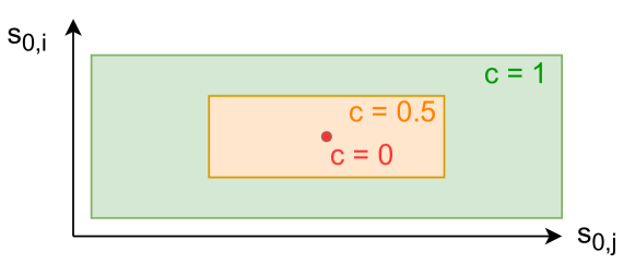
Figure 2: Visualization of the effect of parameter $c$ on $\mu_{0}$.

Important to note, our E2H-ISE formulation is inherently different from  [15, 16, 17] as our solution does not concentrate on goal difficulty but the entropy of $\mu_{0}$. In our case, the easy2hard attribute derives from the magnitude of the entropy and not from the goal difficulty. It is also disparate from [20] as their solution maximizes the entropy of goal-conditioned visited states $\mathcal{H}(\mathcal{S}|\mathcal{G})$ and not $\mathcal{H}(\mu_{0})$.

IV-C HiER+

In this section, HiER+ is presented which is a combination of HiER and E2H-ISE, and can be added to any off-policy RL algorithm with or without HER and PER, depicted in Fig. 1 and presented in Algorithm 1. Having initialized the variables and the environment (Lines 1-6), the training loop starts. After collecting an episode, its transitions are stored in $\mathcal{B}_{ser}$, and if HER is active then virtual experiences are added as well (Lines 13-14). Then the $\lambda$ parameter of HiER is updated and if the given condition is met, the episode is stored in $\mathcal{B}_{hier}$ as well (Lines 15-18). In the next steps, the $c$ parameter of E2H-ISE is updated and the environment is reinitialized (Line 19-21), thus the agent can start collecting the next episode. At a given frequency, the weights of the models are updated (Line 23-31). The batches of $\mathcal{D}_{ser}$ and $\mathcal{D}_{hier}$ are sampled and combined (Lines 24-26). After the weight update (Line 27), if PER is active, the priorities in $\mathcal{B}_{ser}$ are updated (Line 28). Finally, the $\xi$ parameter and with it the batch size of HiER is updated (Lines 29-30).

Algorithm 1 HiER+

1:Initialize $c\leftarrow 0,\ \lambda,\ \xi,\ n,\ \theta,\ \phi$

2:$n_{hier}\leftarrow\xi\cdot n$ $\triangleright$ n: batch size

3:Initialize SER circular buffer $\mathcal{B}_{ser}\leftarrow\emptyset$

4:Initialize HiER circular buffer $\mathcal{B}_{hier}\leftarrow\emptyset$

5:Initialize episode buffer $\mathcal{E}\leftarrow\emptyset$

6:$s\leftarrow\mu_{0}(c_{0})$ $\triangleright$ Init env

7:while Convergence do

8:     $a\leftarrow\pi_{\theta}(s)$ $\triangleright$ Collecting data

9:     $s_{2},r,d\leftarrow$ Env.step($a$)

10:     $\mathcal{E}\leftarrow\mathcal{E}\cup(s,a,s_{2},r,d)$

11:     $s\leftarrow s_{2}$

12:     if Episode ends then

13:         $\mathcal{B}_{ser}\leftarrow\mathcal{B}_{ser}\cup\mathcal{E}$ $\triangleright$ Store transitions of $\mathcal{E}$

14:         $\mathcal{B}_{ser}\leftarrow\mathcal{B}_{ser}\cup\mathcal{E}_{virtual}$ $\triangleright$ HER (optional)

15:         Update $\lambda_{j}$ $\triangleright$ HiER: Section IV-A

16:         if $\lambda_{j}<\sum_{r_{i}\in\mathcal{E}}r_{i}$ then

17:              $\mathcal{B}_{hier}\leftarrow\mathcal{B}_{hier}\cup\mathcal{E}$

18:         end if

19:         Update $c_{j}$ $\triangleright$ E2H-ISE: Section IV-B

20:         $\mathcal{E}\leftarrow\emptyset$

21:         $s\leftarrow\mu_{0}(c_{j})$

22:     end if

23:     if Weight update then

24:         $\mathcal{D}_{ser}\leftarrow$ select $(n-n_{hier})$ sample from $\mathcal{B}_{ser}$

25:         $\mathcal{D}_{hier}\leftarrow$ select $n_{hier}$ sample from $\mathcal{B}_{hier}$

26:         $\mathcal{D}\leftarrow\mathcal{D}_{cer}+\mathcal{D}_{hier}$

27:         Update weights $\theta,\ \phi$ based on $\mathcal{D}$

28:         Update priorities in $\mathcal{B}_{ser}$ $\triangleright$ PER (optional)

29:         Update $\xi_{k}$ $\triangleright$ HiER: Section IV-A

30:         $n_{hier}\leftarrow\xi_{k}\cdot n$

31:     end if

32:     if Evaluation then

33:         Evaluate agent with $\mu_{0}(c=1)$ $\triangleright$ Standard init

34:     end if

35:end while

V Results

Our contributions were validated on the panda-gym robotic benchmark [35]. Three robotic manipulation tasks were considered:

• Push: A block needs to be pushed to a target.

• Slide: A puck needs to be slid to a target outside of the robot’s reach.

• Pick-and-place: A block needs to be moved to a target that is not necessarily on the table thus the robot needs to grasp the block.

For further details, we refer the reader to [35].

Our method is validated with SAC, except in Section V-D where our method is tested with TD3 and DDPG. The standard hyperparameters are set as default in [36] except the discount factor $\gamma=0.95$ as in [35], and the SAC entropy maximization term $\alpha=0.1$. The buffer size of $\mathcal{B}_{hier}$ was set to $10^{6}$.

In this section, the quantitative results are presented, for qualitative evaluation we refer the reader to the project site.

V-A State-of-the-art

The comparison with the state-of-the-art is presented in Tab. I. On the left side of the header, the components of the specific experiment are displayed (HER, PER, E2H-ISE, HiER). In all the experiments, E2H-ISE was used with the self-paced option while HiER was with predefined $\lambda$ profile. The $\xi$ was prioritized when PER was active and fix with $\xi=0.5$ otherwise. The most relevant configurations are depicted in Fig. 3 as well. Both HiER (blue) and E2H-ISE (green) surpass the baselines (gray) for all tasks. Their combination, HiER+ (purple and magenta) further improves the results and significantly outperforms the state-of-the-art. The best performing HiER+ configuration (with HER and without PER) achieves 1.0, 0.83, and 0.69 mean best success rates compared to its baseline with 0.97, 0.38, and 0.27 scores.

	Components				Push			Slide			Pick-and-place
	HER	PER	E2H-ISE	HiER	Max $\uparrow$	Mean $\uparrow$	Std $\downarrow$	Max $\uparrow$	Mean $\uparrow$	Std $\downarrow$	Max $\uparrow$	Mean $\uparrow$	Std $\downarrow$
Baselines	-	-	-	-	0.21	0.16	0.03	0.34	0.12	0.13	0.09	0.07	0.01
	✓	-	-	-	0.99	0.97	0.02	0.45	0.38	0.04	0.32	0.27	0.03
	-	✓	-	-	0.43	0.26	0.07	0.42	0.25	0.14	0.10	0.08	0.01
	✓	✓	-	-	0.97	0.93	0.03	0.43	0.37	0.02	0.33	0.28	0.02
E2H-ISE	-	-	✓	-	0.95	0.85	0.06	0.47	0.45	0.02	0.30	0.25	0.03
	✓	-	✓	-	1.00	1.00	0.01	0.52	0.45	0.03	0.53	0.42	0.04
	-	✓	✓	-	0.89	0.83	0.04	0.52	0.44	0.04	0.36	0.31	0.03
	✓	✓	✓	-	1.00	0.99	0.01	0.50	0.46	0.03	0.44	0.39	0.03
HiER	-	-	-	✓	0.57	0.44	0.09	0.39	0.29	0.07	0.11	0.09	0.01
	✓	-	-	✓	1.00	1.00	0.00	0.91	0.79	0.09	0.42	0.39	0.02
	-	✓	-	✓	0.98	0.80	0.15	0.66	0.41	0.17	0.16	0.13	0.02
	✓	✓	-	✓	1.00	0.98	0.01	0.83	0.78	0.05	0.39	0.37	0.02
HiER+	-	-	✓	✓	1.00	0.98	0.01	0.76	0.53	0.12	0.39	0.33	0.03
	✓	-	✓	✓	1.00	1.00	0.00	0.95	0.83	0.05	0.90	0.69	0.14
	-	✓	✓	✓	1.00	0.98	0.02	0.65	0.51	0.07	0.50	0.41	0.05
	✓	✓	✓	✓	1.00	1.00	0.00	0.88	0.84	0.05	0.55	0.47	0.06

TABLE I: Our method compared to the state-of-the-art based on the evaluation success rate. The experiments were run with 10 independent random seeds. The Max column shows the single best evaluation result, the Mean column shows the mean of the best evaluation results, and the Std column shows the standard deviation on the best evaluation results. The column-wise best results are marked in bold.

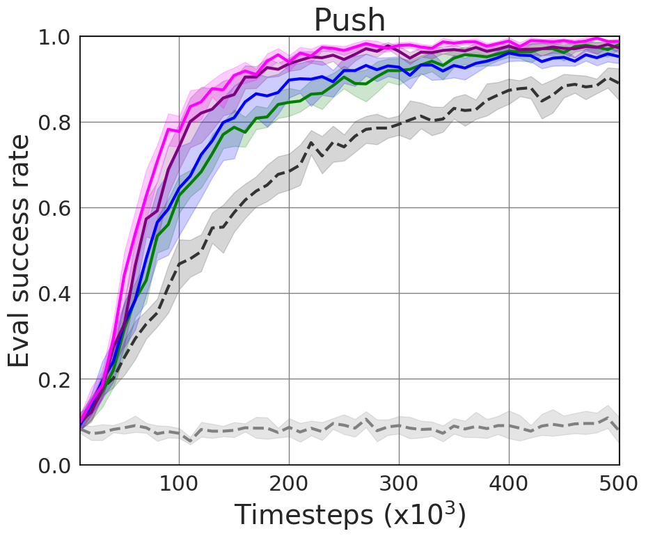
(a)

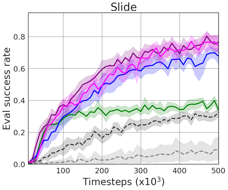
(b)

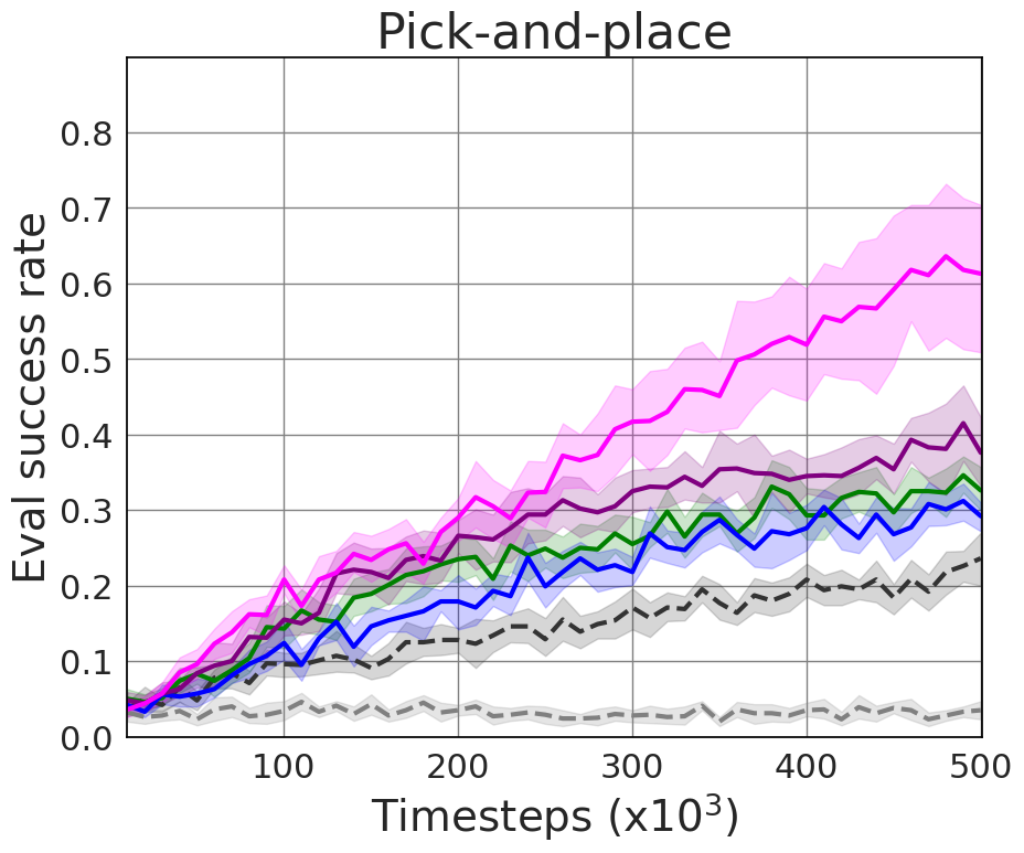
(c)

(d)

Figure 3: Our method compared to the state-of-the-art based on the evaluation success rate. All the results are plotted with their 95% confidence interval, 10 independent seeds in each case.

V-B HiER versions

The different versions of HiER concerning $\lambda$ and $\xi$ are presented in Fig. 4, henceforth referred to as HiER $\lambda$ and HiER $\xi$ versions.

Regarding HiER $\lambda$, the experiments were executed without HER, PER, and E2H-ISE. In these settings, the predefined version outperforms the other variants, depicted in Fig.4 (a), indicating that gradually increasing $\lambda$ could be beneficial. The change of $\lambda$ is depicted in Fig. 4 (b).

The impact of HiER $\xi$ is shown in Fig. 4 (c). The experiments were executed with HER and E2H-ISE but without PER. In these settings, fix $\xi=0.25$ appears to be the best, although we found $\xi=0.5$ better in other settings. Important to note, that when PER is active, it scales the gradient proportionally to the probability of the samples, thus prioritized $\xi$ mode is recommended to counterbalance this effect.

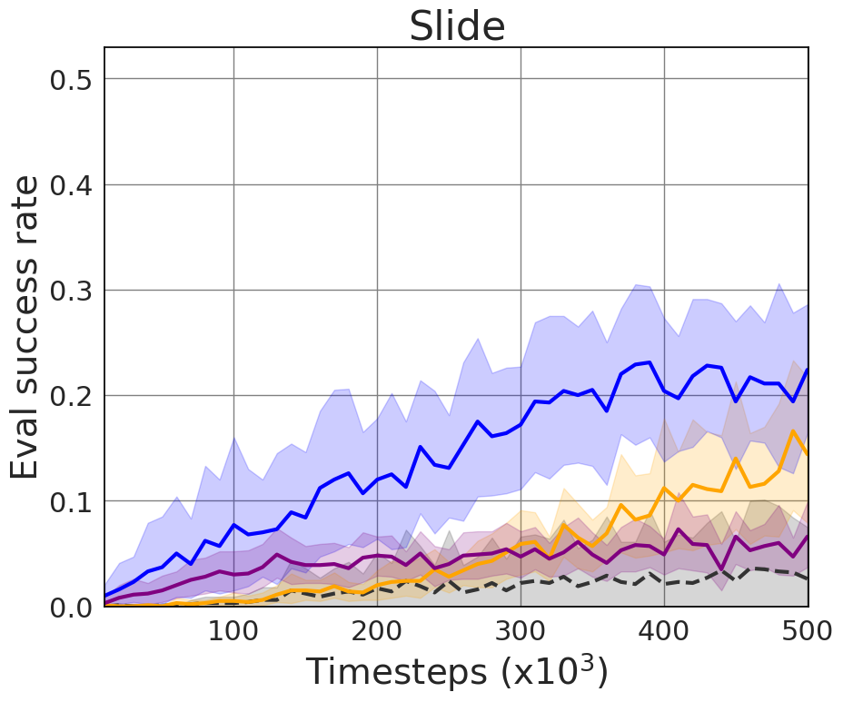
(a) The effect of HiER $\lambda$ versions on the success rate. $\xi$ is fixed at 0.5.

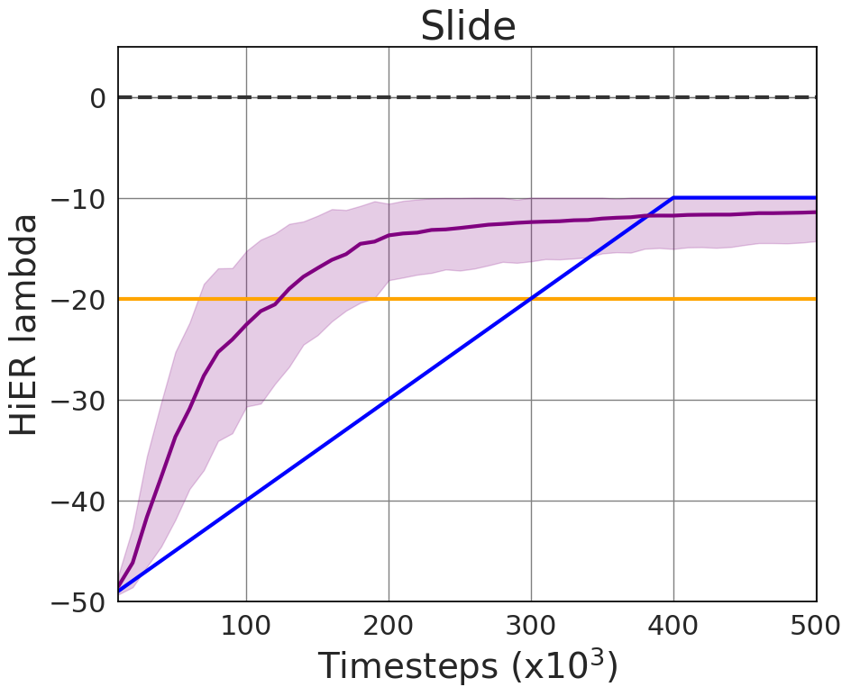
(b) The change of $\lambda$ values over time. $\xi$ is fixed at 0.5.

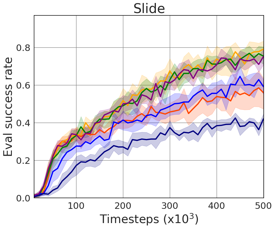
(c) The effect of HiER $\xi$ methods. HiER $\lambda$ is set to predefined.

Figure 4: The effect of HiER $\lambda$ versions (a) and (b), and HiER $\xi$ versions (c). HiER $\lambda$ ama parameters: $\lambda_{0}=-50$, $\lambda_{max}=-10$ $M=0$ and $w=20$. The without version indicates that HiER was not used. All the results are plotted with their 95% confidence interval, 10 independent seeds in each case.

V-C E2H-ISE versions

The different E2H-ISE versions are presented on Tab. II. The experiments were executed without PER as this configuration seems to be superior. The ranking of E2H-ISE versions is relatively sensible for the applied methods (HER and HiER). While without HiER the predefined version had the best mean success rate, with HiER, its performance improved less compared to the other versions. All in all, on average, seemingly the self-paced version performs the best. Nevertheless, further optimization, or possibly another version of E2H-ISE could improve the performance.

Components		predefined			self-paced			control			control adaptive
HER	HiER	Max $\uparrow$	Mean $\uparrow$	Std $\downarrow$	Max $\uparrow$	Mean $\uparrow$	Std $\downarrow$	Max $\uparrow$	Mean $\uparrow$	Std $\downarrow$	Max $\uparrow$	Mean $\uparrow$	Std $\downarrow$
-	-	0.52	0.46	0.03	0.46	0.43	0.02	0.46	0.44	0.02	0.51	0.45	0.03
✓	-	0.49	0.46	0.03	0.54	0.45	0.03	0.53	0.47	0.04	0.54	0.45	0.04
-	✓	0.63	0.50	0.06	0.69	0.49	0.07	0.95	0.57	0.17	0.90	0.55	0.14
✓	✓	0.85	0.71	0.08	0.90	0.81	0.06	0.87	0.70	0.08	0.90	0.80	0.05

TABLE II: The effect of the E2H-ISE methods on the eval success rate. HiER parameters: $\lambda$ mode predefined and $\xi$ fix with $\xi=0.5$. E2H-ISE parameters: self-paced $\Psi_{low}=0.2$, $\Psi_{high}=0.8$ and $\delta=0.05$; control: $\psi=0.8$ and $\delta=0.01$; control adaptive: $\Delta=0.2$, $\psi_{max}=0.9$, and $\delta=0.01$. The row-wise best results are marked in bold. The experiments were run with 10 independent random seeds. Notation is the same as in Tab. I.

V-D TD3 and DDPG

To validate our methods not only with SAC, Tab.III shows our results in the case of DDPG and TD3. The parameters of HiER+ were as in Section V-A. In both cases, HiER+ improved the results of the baseline. Nevertheless, a thorough ablation study on TD3 and DDPG is out of the scope of this paper.

		Push			Slide			Pick-and-place
	Algorithm	Max $\uparrow$	Mean $\uparrow$	Std $\downarrow$	Max $\uparrow$	Mean $\uparrow$	Std $\downarrow$	Max $\uparrow$	Mean $\uparrow$	Std $\downarrow$
TD3	Baseline	0.86	0.40	0.28	0.44	0.27	0.16	0.11	0.09	0.01
	HiER+	0.99	0.93	0.04	0.63	0.53	0.08	0.35	0.28	0.05
DDPG	Baseline	0.42	0.25	0.08	0.74	0.56	0.11	0.11	0.08	0.01
	HiER+	0.91	0.43	0.27	0.83	0.63	0.22	0.20	0.13	0.03

TABLE III: Our method compared to the state-of-the-art based on success rate in the case of TD3 and DDPG. The best results are marked in bold. The experiments were run with 10 independent random seeds. Notation is the same as in Tab. I.

VI Conclusion

In this work, we introduced novel techniques called 1.) highlight experience replay, 2.) easy2hard initial state entropy, and 3.) their combination, HiER+ to facilitate the training of off-policy RL agents in a robotic, sparse-reward environment with continuous state and action spaces.

We showed that both HiER and E2H-ISE surpass the baselines, and HiER+ further improves the results, significantly outperforming the state-of-the-art. Its best configuration achieved 1.0, 0.83, and 0.69 evaluation success rates on the push, slide, and pick-and-place robotic manipulation tasks of the panda-gym benchmark.

Furthermore, we presented our experiments on the different versions of HiER and E2H-ISE. On one hand, we found that in the case of HiER $\lambda$, the predefined version was superior. On the other hand, the ranking of the HiER $\xi$ versions and equally the E2H-ISE versions are less straightforward.

We also showed that HiER+ works well not only with SAC but with TD3 and DDPG as well.

For future work, we will investigate other possible HiER and E2H-ISE versions. Moreover, we are interested in how HiER+ could facilitate sim2real knowledge transfer.

References

- [1] K. Weiss, T. M. Khoshgoftaar, and D. Wang, “A Survey of Transfer Learning,” Journal of Big Data, vol. 3, no. 1, p. 9, Dec. 2016. [Online]. Available: http://doi.org/10.1186/s40537-016-0043-6
- [2] D. Horváth, G. Erdős, Z. Istenes, T. Horváth, and S. Földi, “Object Detection Using Sim2Real Domain Randomization for Robotic Applications,” IEEE Transactions on Robotics, vol. 39, pp. 1225–1243, Apr. 2023. [Online]. Available: http://doi.org/10.1109/TRO.2022.3207619
- [3] D. Horváth, K. Bocsi, G. Erdős, and Z. Istenes, “Sim2Real Grasp Pose Estimation for Adaptive Robotic Applications,” IFAC-PapersOnLine, vol. 56, no. 2, pp. 5233–5239, Jan. 2023. [Online]. Available: http://doi.org/10.1016/j.ifacol.2023.10.121
- [4] S. Zhou, M. K. Helwa, A. P. Schoellig, A. Sarabakha, and E. Kayacan, “Knowledge Transfer Between Robots with Similar Dynamics for High-Accuracy Impromptu Trajectory Tracking,” in 2019 18th European Control Conference (ECC), Jun. 2019, pp. 1–8. [Online]. Available: http://doi.org/10.23919/ECC.2019.8796140
- [5] Y. Bao, Y. Li, S.-L. Huang, L. Zhang, L. Zheng, A. Zamir, and L. Guibas, “An Information-Theoretic Approach to Transferability in Task Transfer Learning,” in 2019 IEEE International Conference on Image Processing (ICIP), Sep. 2019, pp. 2309–2313, iSSN: 2381-8549. [Online]. Available: http://doi.org/10.1109/ICIP.2019.8803726
- [6] D. Silver, G. Lever, N. Heess, T. Degris, D. Wierstra, and M. Riedmiller, “Deterministic Policy Gradient Algorithms,” in Proceedings of the 31st International Conference on Machine Learning, ser. Proceedings of Machine Learning Research, E. P. Xing and T. Jebara, Eds., vol. 32, no. 1. Bejing, China: PMLR, 22–24 Jun 2014, pp. 387–395. [Online]. Available: https://proceedings.mlr.press/v32/silver14.html
- [7] T. P. Lillicrap, J. J. Hunt, A. Pritzel, N. Heess, T. Erez, Y. Tassa, D. Silver, and D. Wierstra, “Continuous Control with Deep Reinforcement Learning,” Jul. 2019, arXiv:1509.02971 [cs, stat]. [Online]. Available: http://doi.org/10.48550/arXiv.1509.02971
- [8] S. Fujimoto, H. van Hoof, and D. Meger, “Addressing Function Approximation Error in Actor-Critic Methods,” Oct. 2018, arXiv:1802.09477 [cs, stat]. [Online]. Available: http://doi.org/10.48550/arXiv.1802.09477
- [9] T. Haarnoja, A. Zhou, P. Abbeel, and S. Levine, “Soft Actor-Critic: Off-Policy Maximum Entropy Deep Reinforcement Learning with a Stochastic Actor,” Aug. 2018, arXiv:1801.01290 [cs, stat]. [Online]. Available: http://doi.org/10.48550/arXiv.1801.01290
- [10] D. Silver, T. Hubert, J. Schrittwieser, I. Antonoglou, M. Lai, A. Guez, M. Lanctot, L. Sifre, D. Kumaran, T. Graepel, T. Lillicrap, K. Simonyan, and D. Hassabis, “Mastering Chess and Shogi by Self-Play with a General Reinforcement Learning Algorithm,” Dec. 2017, arXiv:1712.01815 [cs]. [Online]. Available: http://doi.org/10.48550/arXiv.1712.01815
- [11] D. Silver, J. Schrittwieser, K. Simonyan, I. Antonoglou, A. Huang, A. Guez, T. Hubert, L. Baker, M. Lai, A. Bolton, Y. Chen, T. Lillicrap, F. Hui, L. Sifre, G. van den Driessche, T. Graepel, and D. Hassabis, “Mastering the Game of Go without Human Knowledge,” Nature, vol. 550, no. 7676, pp. 354–359, Oct. 2017, number: 7676 Publisher: Nature Publishing Group. [Online]. Available: https://doi.org/10.1038/nature24270
- [12] V. Mnih, K. Kavukcuoglu, D. Silver, A. A. Rusu, J. Veness, M. G. Bellemare, A. Graves, M. Riedmiller, A. K. Fidjeland, G. Ostrovski, S. Petersen, C. Beattie, A. Sadik, I. Antonoglou, H. King, D. Kumaran, D. Wierstra, S. Legg, and D. Hassabis, “Human-Level Control Through Deep Reinforcement Learning,” Nature, vol. 518, no. 7540, pp. 529–533, Feb. 2015, number: 7540 Publisher: Nature Publishing Group. [Online]. Available: https://doi.org/10.1038/nature14236
- [13] B. Mehta, M. Diaz, F. Golemo, C. J. Pal, and L. Paull, “Active Domain Randomization,” Jul. 2019, arXiv:1904.04762 [cs]. [Online]. Available: http://doi.org/10.48550/arXiv.1904.04762
- [14] S. Luo, H. Kasaei, and L. Schomaker, “Accelerating Reinforcement Learning for Reaching Using Continuous Curriculum Learning,” in 2020 International Joint Conference on Neural Networks (IJCNN), Jul. 2020, pp. 1–8, iSSN: 2161-4407. [Online]. Available: https://doi.org/10.1109/IJCNN48605.2020.9207427
- [15] C. Florensa, D. Held, M. Wulfmeier, M. Zhang, and P. Abbeel, “Reverse Curriculum Generation for Reinforcement Learning,” Jul. 2018, arXiv:1707.05300 [cs]. [Online]. Available: http://doi.org/10.48550/arXiv.1707.05300
- [16] B. Ivanovic, J. Harrison, A. Sharma, M. Chen, and M. Pavone, “BaRC: Backward Reachability Curriculum for Robotic Reinforcement Learning,” in 2019 International Conference on Robotics and Automation (ICRA), May 2019, pp. 15–21, iSSN: 2577-087X. [Online]. Available: https://doi.org/10.1109/ICRA.2019.8794206
- [17] T. Salimans and R. Chen, “Learning Montezuma’s Revenge from a Single Demonstration,” Dec. 2018, arXiv:1812.03381 [cs, stat]. [Online]. Available: http://doi.org/10.48550/arXiv.1812.03381
- [18] S. Sukhbaatar, Z. Lin, I. Kostrikov, G. Synnaeve, A. Szlam, and R. Fergus, “Intrinsic Motivation and Automatic Curricula via Asymmetric Self-Play,” Apr. 2018, arXiv:1703.05407 [cs]. [Online]. Available: http://doi.org/10.48550/arXiv.1703.05407
- [19] C. Florensa, D. Held, X. Geng, and P. Abbeel, “Automatic Goal Generation for Reinforcement Learning Agents,” Jul. 2018, arXiv:1705.06366 [cs]. [Online]. Available: http://doi.org/10.48550/arXiv.1705.06366
- [20] V. H. Pong, M. Dalal, S. Lin, A. Nair, S. Bahl, and S. Levine, “Skew-Fit: State-Covering Self-Supervised Reinforcement Learning,” Aug. 2020, arXiv:1903.03698 [cs, stat]. [Online]. Available: http://doi.org/10.48550/arXiv.1903.03698
- [21] S. Racaniere, A. K. Lampinen, A. Santoro, D. P. Reichert, V. Firoiu, and T. P. Lillicrap, “Automated Curricula Through Setter-Solver Interactions,” Jan. 2020, arXiv:1909.12892 [cs, stat]. [Online]. Available: http://doi.org/10.48550/arXiv.1909.12892
- [22] T. Schaul, J. Quan, I. Antonoglou, and D. Silver, “Prioritized Experience Replay,” Feb. 2016, arXiv:1511.05952 [cs]. [Online]. Available: http://doi.org/10.48550/arXiv.1511.05952
- [23] J. Oh, Y. Guo, S. Singh, and H. Lee, “Self-Imitation Learning,” Jun. 2018, arXiv:1806.05635 [cs, stat]. [Online]. Available: http://doi.org/10.48550/arXiv.1806.05635
- [24] J. Ferret, O. Pietquin, and M. Geist, “Self-Imitation Advantage Learning,” Dec. 2020, arXiv:2012.11989 [cs]. [Online]. Available: http://doi.org/10.48550/arXiv.2012.11989
- [25] C. Wang and K. Ross, “Boosting Soft Actor-Critic: Emphasizing Recent Experience without Forgetting the Past,” Jun. 2019, arXiv:1906.04009 [cs, stat]. [Online]. Available: http://doi.org/10.48550/arXiv.1906.04009
- [26] M. Andrychowicz, F. Wolski, A. Ray, J. Schneider, R. Fong, P. Welinder, B. McGrew, J. Tobin, O. Pieter Abbeel, and W. Zaremba, “Hindsight Experience Replay,” in Advances in Neural Information Processing Systems, vol. 30. Curran Associates, Inc., 2017. [Online]. Available: https://doi.org/10.48550/arXiv.1707.01495
- [27] J. Bujalance and F. Moutarde, “Reward Relabelling for Combined Reinforcement and Imitation Learning on Sparse-Reward Tasks,” in Proceedings of the 2023 International Conference on Autonomous Agents and Multiagent Systems, 2023, pp. 2565–2567. [Online]. Available: https://doi.org/10.48550/arXiv.2201.03834
- [28] Y. Bengio, J. Louradour, R. Collobert, and J. Weston, “Curriculum learning,” in Proceedings of the 26th Annual International Conference on Machine Learning, ser. ICML ’09. New York, NY, USA: Association for Computing Machinery, Jun. 2009, pp. 41–48. [Online]. Available: https://doi.org/10.1145/1553374.1553380
- [29] R. Portelas, C. Colas, L. Weng, K. Hofmann, and P.-Y. Oudeyer, “Automatic Curriculum Learning For Deep RL: A Short Survey,” May 2020, arXiv:2003.04664 [cs, stat]. [Online]. Available: http://doi.org/10.48550/arXiv.2003.04664
- [30] X. Wang, Y. Chen, and W. Zhu, “A Survey on Curriculum Learning,” IEEE Transactions on Pattern Analysis and Machine Intelligence, vol. 44, no. 9, pp. 4555–4576, Sep. 2022, conference Name: IEEE Transactions on Pattern Analysis and Machine Intelligence. [Online]. Available: http://doi.org/10.1109/TPAMI.2021.3069908
- [31] T. Schaul, D. Horgan, K. Gregor, and D. Silver, “Universal Value Function Approximators,” in Proceedings of the 32nd International Conference on Machine Learning, ser. Proceedings of Machine Learning Research, F. Bach and D. Blei, Eds., vol. 37. Lille, France: PMLR, 07–09 Jul 2015, pp. 1312–1320. [Online]. Available: https://proceedings.mlr.press/v37/schaul15.html
- [32] A. Shrivastava, A. Gupta, and R. Girshick, “Training Region-Based Object Detectors with Online Hard Example Mining,” in 2016 IEEE Conference on Computer Vision and Pattern Recognition (CVPR). Las Vegas, NV, USA: IEEE, Jun. 2016, pp. 761–769. [Online]. Available: http://doi.org/10.1109/CVPR.2016.89
- [33] R. S. Sutton, “Learning to Predict by the Methods of Temporal Differences,” Machine Learning, vol. 3, no. 1, pp. 9–44, Aug. 1988. [Online]. Available: https://doi.org/10.1007/BF00115009
- [34] D. Kumaran, D. Hassabis, and J. L. McClelland, “What Learning Systems do Intelligent Agents Need? Complementary Learning Systems Theory Updated,” Trends in Cognitive Sciences, vol. 20, no. 7, pp. 512–534, Jul. 2016. [Online]. Available: https://doi.org/10.1016/j.tics.2016.05.004
- [35] Q. Gallouédec, N. Cazin, E. Dellandréa, and L. Chen, “Panda-Gym: Open-Source Goal-Conditioned Environments for Robotic Learning,” Dec. 2021, arXiv:2106.13687 [cs]. [Online]. Available: http://doi.org/10.48550/arXiv.2106.13687
- [36] “Soft Actor-Critic — Spinning Up documentation.” [Online]. Available: https://spinningup.openai.com/en/latest/algorithms/sac.html