Modeling and Predicting Epidemic Spread: A Gaussian Process Regression Approach

Abstract

Modeling and prediction of epidemic spread are critical to assist in policy-making for mitigation. Therefore, we present a new method based on Gaussian Process Regression to model and predict epidemics, and it quantifies prediction confidence through variance and high probability error bounds. Gaussian Process Regression excels in using small datasets and providing uncertainty bounds, and both of these properties are critical in modeling and predicting epidemic spreading processes with limited data. However, the derivation of formal uncertainty bounds remains lacking when using Gaussian Process Regression in the setting of epidemics, which limits its usefulness in guiding mitigation efforts. Therefore, in this work, we develop a novel bound on the variance of the prediction that quantifies the impact of the epidemic data on the predictions we make. Further, we develop a high probability error bound on the prediction, and we quantify how the epidemic spread, the infection data, and the length of the prediction horizon all affect this error bound. We also show that the error stays below a certain threshold based on the length of the prediction horizon. To illustrate this framework, we leverage Gaussian Process Regression to model and predict COVID-19 using real-world infection data from the United Kingdom.

1 Introduction

Modeling the spread of diseases is critical for understanding spreading patterns (Giordano et al., 2020). Forecasting how diseases spread is a key element in the study of spreading dynamics and assists in decision-making for epidemic mitigation (Woolhouse, 2011). Existing epidemic modeling and prediction techniques typically construct spreading models by selecting appropriate model structures and parameters to fit real-world spreading data (Gallo Marin et al., 2021; Rahimi et al., 2021; Wynants et al., 2020). However, constructing spreading models can be challenging, especially when dealing with limited data, complex spreading patterns, time-varying parameters, intricate network structures, and uncertainties related to population behavior (Roda et al., 2020). To overcome these challenges, researchers have explored alternative approaches. For instance, researchers have used disease spread metrics that can be obtained from spreading data directly, such as the exponential growth rate (Merow and Urban, 2020), the reproduction number (Cori et al., 2013), and the daily infected/hospitalized/deceased cases (Anastassopoulou et al., 2020; Talkhi et al., 2021) to study the severity of disease spread. Inspired by these ideas, we study how to analyze the trend in disease spreading by modeling and predicting the number of infected cases.

The number of infected cases is a widely accepted metric for assessing epidemic spreading processes because it captures the severity of the epidemic directly (Wu et al., 2020). Consequently, it is common to use past spreading data as feedback information to notify the public and guide decision-making for policymakers (Casella, 2020; She et al., 2022b). To make decisions that mitigate pandemic spread in the near future, predicting the change in the number of the infected cases is also critical, in part because such predictions can facilitate predictive control analysis to allocate resources optimally (Maciejowski and Huzmezan, 2007).

Prediction mechanisms can depend on parametric and non-parametric methods. Leveraging parametric models usually depends on fitting spreading data to a specific epidemic compartmental model. For example, Alsayed et al. (2020) propose a Genetic Algorithm to estimate the parameters of the Susceptible–Exposed–Infectious–Recovered (SEIR) model to further predict the number of the infected cases. Meanwhile, Khajanchi and Sarkar (2020) forecast the daily and cumulative number of cases for the COVID-19 pandemic in India through a compartmental model with seven compartments. To implement a model-predictive control framework for epidemic mitigation, She et al. (2022a) leverage linear regression to estimate the parameters for an SIR model to predict future infections. However, parametric models may not be robust to model uncertainties, since the spreading behavior is complex (Wilke and Bergstrom, 2020). Compared to parametric models, non-parametric models have the advantage of modeling and predicting an infection without a predefined model structure. For instance, (Wang et al., 2019; Wu et al., 2018; Alazab et al., 2020; Datilo et al., 2019) leverage neural networks to forecast epidemic spread. However, artificial intelligence methods such as neural networks may require large training datasets that can be difficult to obtain. In addition, the lack of formal prediction uncertainty analysis makes it challenging for these approaches to guide policy-making.

In order to tackle this challenge, we leverage Gaussian Process Regression to model and predict the number of infected cases, where we not only provide uncertainty guarantees for the prediction but also illustrate the results with application to real-world epidemic spread. Gaussian Process Regression excels at capturing complex, nonlinear relationships without relying on predefined functional forms and can effectively handle small datasets (Williams and Rasmussen, 2006). For instance, Senanayake et al. (2016) use variational Gaussian Process Regression to model and predict the seasonal change of Influenza. Meanwhile, Velásquez and Lara (2020) use reduced-space Gaussian Process Regression to forecast the COVID-19 spread in the USA. Similarly, Ketu and Mishra (2021) propose a Multi-Task Gaussian Process (MTGP) Regression model to predict the COVID-19 outbreak worldwide.

Although the use of a Gaussian Process Regression model for disease spread modeling and prediction is not new, most work that utilizes Gaussian Process Regression does not provide a rigorous analysis of model and prediction uncertainty. This lack of rigor makes it challenging to guide real-world decision-making (Hewing et al., 2020). Therefore, we provide a new way to model the change in the number of the infected cases through Gaussian Process Regression, where we are able to provide insights into the uncertainty of the predictions that it produces. We propose an upper bound on the variance of the prediction to study the impact of the epidemic data on the prediction. Further, we develop a high probability error bound on the prediction, where we study how the epidemic spread, the infection data, and the length of the prediction affect the error bound. These results take a critical step in facilitating the development of rigorous predictive control approaches for epidemic mitigation in future works.

In summary, we leverage Gaussian Process Regression to model and predict epidemic spread based on time-series infection data, and we rigorously quantify the model and prediction uncertainty. We bridge the gap between (i) the theoretical analysis of using Gaussian Process Regression for modeling and predicting epidemic spread, and (ii) its practical application in epidemic mitigation. In particular, we use real COVID-19 data from the United Kingdom to illustrate the Gaussian Process Regression model. The rest of the paper is organized as follows. Section II provides background and problem statements. Section III proposes the model and analyzes the impact of data on prediction uncertainty. Section IV illustrates the model by leveraging COVID-19 data from the United Kingdom.

Notation

We use $\mathbb{R}$ and $\mathbb{N}$ to denote the sets of real numbers and natural numbers, respectively. We use $\underline{n}$ to denote the set $\{1,2,\dots,n\}$, $n\in\mathbb{N}_{>0}$. In addition, we use $Card(S)$ to denote the cardinality of a finite set $S$. For a real symmetric matrix $A\in\mathbb{R}^{n\times n}$, we use $[A]_{ij}$ to denote its entry on the $i^{th}$ row and $j^{th}$ column. We use $\lambda_{\max}(A)$ to denote its largest eigenvalue. We use $I_{n}\in\mathbb{R}^{n\times n}$ to denote the identity matrix. Let $\mathcal{N}(\mu,\sigma^{2})$ denote the one dimensional normal distribution with the mean $\mu$ and variance $\sigma^{2}$. We use $\exp(\cdot)$ and $\log(\cdot)$ to denote the exponential function and the logarithmic functions, respectively. We use $p(\cdot)$ to represent the probability distribution of a random variable.

2 Background and Problem Formulation

In this section, we first introduce Gaussian Process Regression. Then we introduce epidemic spread. Finally, we formally state the problem that we address in the remainder of the paper.

2.1 Gaussian Process Regression

We briefly introduce one-dimensional Gaussian Process Regression (Williams and Rasmussen, 2006). Consider an unknown function $f:\mathbb{R}\rightarrow\mathbb{R}$ and $n$ inputs captured by $X=[x_{1},\dots,x_{n}]^{\top}\in\mathbb{R}^{n}$, $n\in\mathbb{N}_{>0}$. The corresponding outputs are given by the vector $F=[f(x_{1}),\dots,f(x_{n})]^{\top}\in\mathbb{R}^{n}$, where the $n$ outputs in $F$ follow a jointly Gaussian distribution. The mean of the jointly Gaussian distribution is given by $m(X)=[m(x_{1}),\cdots,m(x_{n})]^{\top}$, where $m(x_{i})\in\mathbb{R}$, $i\in\underline{n}$. Further, the covariance is given by the kernel function $k:\mathbb{R}\times\mathbb{R}\rightarrow\mathbb{R}_{\geq 0}$, $i,j\in\underline{n}$, where $k(x_{i},x_{j})$ is the covariance between $x_{i}$ and $x_{j}$. Consider that the observation of each output $f(x_{i})$ is corrupted with zero-mean independent Gaussian noise, i.e., $y(x_{i})=f(x_{i})+\epsilon$, where $\epsilon\sim\mathcal{N}(0,\sigma^{2})$, and $\sigma^{2}$ denotes the variance of the noise term $\epsilon$. We define the covariance matrix of the noise as $\sigma^{2}I_{n}\in\mathbb{R}^{n\times n}$. Using the training dataset of $n\in\mathbb{N}_{>0}$ input-output pairs $\{(x_{i},y(x_{i}))\}_{i=1}^{n}$, we can employ Gaussian Process Regression to model the input-output relation $f:\mathbb{R}\rightarrow\mathbb{R}$ at the training location $x_{i}$, $i\in\underline{n}$, and to predict the output $f(x^{*})\in\mathbb{R}$ at the testing location $x^{*}\in\mathbb{R}$, where $x^{*}\neq x_{i}$ for all $i\in\underline{n}$.

Gaussian Process Regression is a kernel-based approach. Hence, we use $k(\cdot,\cdot):\mathbb{R}\times\mathbb{R}\rightarrow\mathbb{R}_{\geq 0}$ to represent the potential kernel function we choose for regression (Genton, 2001). Let $K(X,X)\in\mathbb{R}^{n\times n}_{\geq 0}$ denote the kernel matrix of the training points, where $[K(X,X)]_{ij}=k(x_{i},x_{j})$ denotes the covariance between two training points $x_{i}$ and $x_{j}$, for $i,j\in\underline{n}$. For a testing point $x^{*}$, we further define $K(x^{*},X)\in\mathbb{R}^{1\times n}$ as the kernel vector such that $[K(x^{*},X)]_{j}=k(x^{*},x_{j})$, $j\in\underline{n}$. Therefore, $K(x^{*},X)$ captures the covariance function between the testing point $x^{*}$ and the training point $x_{i}$ for all $i\in\underline{n}$. As Gaussian Process Regression operates as a Bayesian inference approach, we consider a zero-mean prior for generality (Williams and Rasmussen, 2006). The value zero in our study serves as a spreading indicator. If the indicator is zero, the spread remains unchanged; if it is greater than zero, then infected cases increase, and if it is less than zero, then infected cases decrease. This indicator functions similarly to the reproduction number (van den Driessche, 2017). Note that the results we develop can be generalized to any other priors. We will further explain the indicator in the next section.

Consider the posterior distribution for the predicted random variable $f(x^{*})$ at the testing location $x^{*}$ conditioned on the noisy training variables $\{y(x_{1}),\cdots,y(x_{n})\}$. The posterior mean $m(x^{*})$ and posterior variance $\sigma^{2}(x^{*})$ at the testing location $x^{*}$ are given by the following result (Williams and Rasmussen, 2006).

Proposition 2.1.

We define $Y=[y(x_{1}),\cdots,y(x_{n})]^{\top}$. Then $f(x^{*})\mid Y$ satisfies $p(f(x^{*})\mid Y)=\mathcal{N}(m_{Y}(x^{*}),\sigma_{Y}^{2}(x^{*}))$, where

$$m_{Y}(x^{*})=K(x^{*},X)(K(X,X)+\Sigma)^{-1}Y,$$

$$\sigma_{Y}^{2}(x^{*})=k(x^{*},x^{*})-K(x^{*},X)(K(X,X)+\Sigma)^{-1}K(x^{*},X)^{\top}.$$

Proposition 2.1 applies to Gaussian Process Regression with zero prior mean and observation noise with constant variance. For applications in modeling and predicting epidemic spreading processes, the covariance functions $k(\cdot,\cdot)$ are typically chosen to scale with how far away any pair of data points are from each other. These properties establish the foundation for investigating the modeling and prediction uncertainty by Gaussian Process Regression.

2.2 Problem Formulation

As discussed in the introduction, critical metrics such as the number of infected cases can be leveraged to assess epidemic spread. However, the number of infected cases at any time step does not follow a Gaussian distribution. Therefore, the first challenge is to propose a reasonable way to model the infected cases through Gaussian Process Regression. In the context of an epidemic spreading process, the severity of the epidemic can be monitored through population testing and data reporting. Although the epidemic spreading process is continuous-time, observations and predictions are limited by data collection and reporting methods, such as measuring cases at daily, weekly, or monthly intervals. The sampling interval, typically determined by authorities, will therefore affect predictions made from testing data. Therefore, we aim to address how the data reporting interval and the length of the prediction horizon into the future affect the prediction error in the regression problem. In summary, in this work, our goal is to propose a way to leverage Gaussian Process Regression to model epidemic spread and then predict its future trajectory. Specifically, we study the following questions:

• 1. How can we leverage Gaussian Process Regression to model epidemic spread by predicting the future spreading trend?

• 2. Is it possible to obtain prediction uncertainty for epidemic spread through Gaussian Process Regression?

• 3. How do factors such as the sampling interval, observation noise, and number of data points impact the prediction variance?

• 4. What role does the spread behavior and the length of the prediction horizon play in leveraging Gaussian Process Regression to predict future spread, particularly in terms of prediction uncertainty?

We will answer these four questions in the next section.

3 Gaussian Process Regression for Predicting Epidemic Spread

We first introduce epidemic dynamics and propose a method to model the spreading trend in Section 3.1. Then, we leverage Gaussian Process Regression to model and predict the dynamics. We develop an upper bound on the prediction variance to study the impact of the infection data in Section 3.2. In Section 3.3, we will develop a high probability error bound for the prediction, where we explain the relationship between the spreading dynamics, the data, and the error bound.

3.1 Modeling the Spread Using Gaussian Process Regression

For an epidemic spreading process, we use $I(t)$ to denote a noisy observation of the number of the infected cases at time step $t\geq 0$, i.e., $I(t)$ is equal to the number of infected cases at time $t$ plus some noise. We use $\bar{I}(t)$, $t\geq 0$, to denote the true infected cases without observation noise, i.e., the latent variable. Consider the data set $\{I(t_{0}),I(t_{1}),\dots,I(t_{n})\}$ that was measured at times $\{t_{0},t_{1},\dots,t_{n}\}$, $n\in\mathbb{N}$. We first solve Problem 1 in Section 2.2 by proposing a model to capture the trend of the disease spread. Inspired by (Abbott et al., 2020), we suppose that the change in the logarithm of the number of the infected cases between pairs of consecutive time steps follows a Gaussian Process. Hence, for $i\in\underline{n}$, we define

$$\Delta_{\eta}(t_{i})=\log I(t_{i})-\log I(t_{i-1})=\underbrace{\log\bar{I}(t_{i})-\log\bar{I}(t_{i-1})}_{\bar{\Delta}_{\eta}(t_{i})}+\epsilon(t_{i}),$$ (1)

where $\eta=t_{i}-t_{i-1}\geq 0$ captures the length of the time interval for sampling the number of infected cases, which is determined by the data collection approach. Note that $\Delta_{\eta}(t_{i})=\log(\frac{I(t_{i})}{I(t_{i-1})})$ captures the ratio between the number of infected cases at time step $t_{i}$ and time step $t_{i-1}=t_{i}-\eta$, for $\eta>0$. Thus, if the number of infected cases is increasing from time step $t_{i-1}$ to $t_{i}$, then $\Delta_{\eta}(t_{i})$ will be greater than $0$, and vice versa. If the number of infected cases stabilizes at a certain value, then $\Delta_{\eta}(t_{i})=0$. Similar to the reproduction number (van den Driessche, 2017), where the change in spreading behavior is captured by the threshold $1$, we can use the threshold of $0$ for $\Delta_{\eta}(t)$ to capture the spread. Therefore, it is meaningful to leverage $\Delta_{\eta}(t)$ to analyze spreading trends. We consider the case where $I(t)>0$. Note that $\eta$ can represent one hour, one day, one week, etc. To simplify the analysis, we use i.i.d noise $\epsilon(t_{i})\sim\mathcal{N}(0,\sigma^{2})$ to capture the noise between the differences of $\log I(t_{i})$ and $\log I(t_{i-1})$.

Remark 3.1.

Sam Abbott et al. (2020) propose a way to predict the change in the logarithm of the infected data (i.e., $\log(t_{i})-\log(t_{i-1})$, for all $i\in\underline{n}$) through Gaussian Process Regression. However, the focus of that work is on developing computational tools for prediction (e.g., relying on Markov chain Monte Carlo methods). Thus, no theoretical analyses of the modeling and prediction are provided. As discussed in the Introduction, one of the important applications of epidemic prediction is to guide decision-making. For designing resource allocation strategies through predictive control algorithms, leveraging the predicted spreading trend as feedback, we need to analyze the model and prediction errors generated through Gaussian Process Regression. Therefore, developing error bounds on the prediction lays a foundation for control design in epidemic mitigation for future work.

For an epidemic spreading process, the numbers of infected cases at consecutive time steps are given by $I=\{I(t_{0}),I(t_{1}),\dots,I(t_{n})\}$, $n\in\mathbb{N}_{>0}$. We consider the set of $n$ time steps $T=\{t_{1},t_{2},\dots,t_{n}\}$ as the input batch. The corresponding output batch of $n$ entries is given by $\Delta=[\Delta_{\eta}(t_{1}),\Delta_{\eta}(t_{2}),\dots,\Delta_{\eta}(t_{n})]^{\top}$, where $\Delta_{\eta}(t_{i})$, $i\in\underline{n}$, is given by (1). Our goal is to model and predict the change in the difference of the logarithm of the infected cases. Hence, let the testing location (at which we predict the epidemic spread) be the time step $t^{*}=t_{n}+\eta d$. The parameter $d\in\mathbb{N}_{>0}$ denotes the length of the prediction horizon, which determines how many time steps we would like to predict in the near future, where time steps are separated by the sampling interval $\eta$. After incorporating the epidemic prediction problem through Gaussian Process Regression, based on Proposition 2.1, we have the following result.

Proposition 3.2.

The prediction mean is given by $m_{\Delta}(t^{*})=K(t^{*},T)(K(T,T)+\sigma^{2}I_{n})^{-1}\Delta$. The variance of the prediction is $\sigma^{2}_{\Delta}(t^{*})=k(t^{*},t^{*})-K(t^{*},T)(K(T,T)+\sigma^{2}I_{n})^{-1}K(t^{*},T)^{\top}$.

Proposition 3.2 addresses the Problem 1 in Section 2.2. In the next subsection, we will develop an upper bound on the prediction variance $\sigma^{2}_{\Delta}(t^{*})$.

3.2 The Impact of Spread Data on Prediction Variance

Proposition 3.2 provides the analytical solution for leveraging Gaussian Process Regression to predict the change in the logarithm of the infection data. To better analyze the performance of the regression, we specify the kernel function used in the regression. Specifically, we use the squared exponential kernel to capture the covariance function between any pair of points $a,b\in\mathbb{R}$, such that

$$k(a,b)=\alpha^{2}\exp\left(-\frac{(a-b)^{2}}{2\beta^{2}}\right),$$ (2)

where $\beta>0$ is the length scale of the kernel, and $\alpha^{2}$ is the signal variance. The length scale captures the strength of the coupling between any pair of points $(a,b)$ with respect to their distance. The signal variance captures the rate at which the function changes in terms of magnitude.

Remark 3.3.

As a widely used kernel in Gaussian Process Regression, the squared exponential kernel is a stationary kernel, implying that the covariance between two random variables at two points depends only on the distance between them, not on their absolute locations. The squared exponential kernel is infinitely differentiable, promoting smoothness in the modeled functions. Moreover, the squared exponential kernel is Lipschitz continuous, a critical property for deriving error bounds in subsequent work (Williams and Rasmussen, 2006). The kernel has also been successfully implemented for epidemic spread prediction (Abbott et al., 2020). Therefore, in this study, we choose the squared exponential kernel as our kernel function for analysis. Note that our results can be generalized when using other stationary kernels with Lipschitz continuity, though we use the squared exponential kernel due to its prior success in epidemic modeling.

We next propose an upper bound for the prediction variance. Consider a set of time steps $T=\{t_{1},t_{2},\dots,t_{n}\}$. Let $\mathbb{T}_{r}(t^{*})$ denote the time interval such that $\mathbb{T}_{r}(t^{*})=\{t|t\in\underset{t_{i}\in T}{\bigcup}(\left|t_{i}-t^{*}\right|\leq r)\}$ contains all time steps in $T$ that are contained within a ball of radius $r$ around the testing location $t^{*}$.

Theorem 3.4.

Let the squared exponential kernel from (2) be used and let $T\subset\mathbb{T}_{r}(t^{*})$. Then the posterior variance $\sigma^{2}_{\Delta}(t^{*})$ at the testing time step $t^{*}$ in Proposition 3.2 is upper bounded by $\alpha^{2}-\frac{\alpha^{4}\exp(-\frac{r^{2}}{\beta^{2}})}{\alpha^{2}\exp(-\frac{\eta^{2}}{2\beta^{2}})+\frac{\sigma^{2}}{n}}$.

Proof 3.5.

Based on Proposition 3.2,

$$\sigma^{2}_{\Delta}(t^{*}) =k(t^{*},t^{*})-K(t^{*},T)(K(T,T)+\sigma^{2}I_{n})^{-1}K(t^{*},T)^{\top}$$

$$\leq k(t^{*},t^{*})-\frac{\|K(t^{*},T)\|^{2}}{\lambda_{\max}(K(T,T)+\sigma^{2}I_{n})}\leq k(t^{*},t^{*})-\frac{\|K(t^{*},T)\|^{2}}{\lambda_{\max}(K(T,T))+\sigma^{2}}.$$

Note that we use the conditions that the covariance matrix $K(T,T)$ is a positive semidefinite matrix and that $\sigma^{2}I_{n}$ is a positive definite diagonal matrix; thus, $K(T,T)+\sigma^{2}I_{n}$ is a positive definite matrix. By applying the Gershgorin Circle Theorem (Gershgorin, 1931), we find

$$\lambda_{\max}(K(T,T))\leq n\underset{\begin{subarray}{c}t_{i},t_{j}\in T,t_{i}\neq t_{j}\end{subarray}}{\max}k(t_{i},t_{j})=n\alpha^{2}\exp(-\frac{\eta^{2}}{2\beta^{2}}).$$ (3)

Here, we use the condition that $\underset{\begin{subarray}{c}t_{i},t_{j},\in T,t_{i}\neq t_{j}\end{subarray}}{\max}k(t_{i},t_{j})$ is obtained where $\underset{\begin{subarray}{c}t_{i},t_{j}\in T,t_{i}\neq t_{j}\end{subarray}}{\min}(t_{i}-t_{j})^{2}$ is obtained, since the value of the squared exponential kernel increases when the interval between the two time steps decreases. Based on the condition that the interval between any pair of time steps of observations and predictions of data are determined by the sampling interval $\eta$, we see that $\eta$ is the minimal length of the time interval $t_{i}-t_{j}$, i.e., we have $\underset{\begin{subarray}{c}t_{i},t_{j}\in T,t_{i}\neq t_{j}\end{subarray}}{\min}(t_{i}-t_{j})^{2}=\eta^{2}$. Therefore, $\underset{t_{i},t_{j}\in T,t_{i}\neq t_{j}}{\max}k(t_{i},t_{j})=\alpha^{2}\exp(-\frac{\eta^{2}}{2\beta^{2}})$, and we obtain (3).

Based on the definition of the kernel vector $K(t^{*},T)$ and (2), we have that

$$\|K(t^{*},T)\|^{2}\geq n~{}\underset{t_{i}\in T}{\min}\ k^{2}(t^{*},t_{i})=n\alpha^{4}\exp(-\frac{r^{2}}{\beta^{2}}).$$ (4)

Similarly, based on the property of the squared exponential kernel, and the condition $T\subset\mathbb{T}_{r}(t^{*})$, it can be observed that solving $\underset{t_{i}\in T}{\operatorname*{arg\,min}}\ k(t_{i},t^{*})$ gives the same answer as solving $\underset{t_{i}\in T}{\operatorname*{arg\,max}}\ (t_{i}-t^{*})^{2}$. Recall that the training and prediction time steps satisfy that $\mathbb{T}_{r}(t^{*})=\{t|t\in\underset{t_{i}\in T}{\bigcup}(\left|t_{i}-t^{*}\right|\leq r)\}$, and thus $T\subset\mathbb{T}_{r}(t^{*})$ and $t^{*}\in\mathbb{T}_{r}(t^{*})$. Hence, $\underset{t_{i}\in T}{\max}\ (t^{*}-t_{i})^{2}=r^{2}$ and $\underset{t_{i}\in T}{\min}\ k^{2}(t^{*},t_{i})=(\alpha^{2}\exp(-\frac{r^{2}}{2\beta^{2}}))^{2}$, and we obtain (4).

In addition, we have that $k(t^{*},t^{*})=\alpha^{2}$. By substituting (3) and (4) in $\sigma^{2}_{\Delta}(t^{*})$, we have

$$\sigma^{2}_{\Delta}(t^{*})\leq\alpha^{2}-\frac{\alpha^{4}\exp(-\frac{r^{2}}{\beta^{2}})}{\alpha^{2}\exp(-\frac{\eta^{2}}{2\beta^{2}})+\frac{\sigma^{2}}{n}},$$

which completes the proof.

Theorem 3.4 provides an upper bound on the prediction variance $\sigma^{2}_{\Delta}(t^{*})$ at the testing time step $t^{*}$, when all training time steps satisfy $T\subset\mathbb{T}_{r}(t^{*})$. In order to further investigate the spread, we provide the following remarks to study the impact of the data on the variance bound. We note the following, which follow by using the monotonicity property of the variance upper bound.

Remark 3.6.

The bound on the prediction variance given by Theorem 3.4 satisfies the following results:

• The more data points we have, captured by $n\in\mathbb{N}_{\geq 0}$, the lower the variance bound.

• The lower the observation noise $\sigma^{2}$ at the training time steps is, the lower the variance bound.

• The higher the sampling step interval $\eta$ is, the lower the variance bound.

Remark 3.7.

Theorem 3.4 and Remark 3.6 illustrate that the way in which we use spread data can affect the variance bound, and thus together they address Problems 2 and 3 in Section 2.2. Note that the variance bound in Remark 3.6 is based on the condition that the training points are restricted to an interval around the testing location $t^{*}$ with a radius $r$, captured by $\mathbb{T}_{r}(t^{*})$. Consequently, the more training data we have in $\mathbb{T}_{r}(t^{*})$, the lower the variance bound. This is intuitive since it implies that having more training data near $t^{*}$ leads to greater confidence in our predictions at $t^{*}$. We also consider the impact of observation noise $\epsilon$, and we see that higher observation noise will result in a higher variance bound for the prediction, which is also intuitive. Thus, it is crucial to design a screening strategy to obtain relatively accurate numbers of infected cases to lower the observation noise.

The last point concerns the length of the sampling interval. We use an example to explain why a higher sampling interval will generate a lower upper bound. Consider $r$ equal to $7$ days. We fix the number of testing points at five, and we consider two scenarios. In the first scenario, where we record infection data every day, we can leverage the daily infected cases to compute $\Delta_{\eta}(t)$ from day $1$ to day $5$ to predict the spread $\Delta_{\eta}(t^{*})$ on day $7$. In the second scenario, where we record infection data every half day, we can use $\Delta_{\eta}(t)$ from day 1 (12 AM) to day 3 (12 AM) to predict $\Delta_{\eta}(t^{*})$ on day $7$. It is natural to think that the first scenario will generate a lower prediction variance since most data points are closer to the testing time step, i.e., day $5$. Mathematically, for an interval $T_{r}(t^{*})$ with a fixed radius $r$, when we choose the number of training time steps as $n$, a higher sampling interval $\eta$ will spread the training data across the interval, while a lower sampling interval $\eta$ will cluster the training data in a smaller interval. Since the upper bound on the prediction variance is a worst-case bound, a more clustered training dataset will result in a higher variance bound. Note that the discussion does not apply to the situation where increasing $\eta$ may decrease the number of training points in an interval of radius $r$ around the testing location $t^{*}$. Therefore, it is important to select an appropriate sampling interval $\eta$ to record infection data that effectively controls the bound on the posterior variance.

3.3 High Probability Error Bound on The Prediction

Having discussed the impact of data on the upper bound of the prediction variance, we now analyze the error bound on the prediction mean. We next introduce the Lipschitz constant on the squared exponential kernel (Lederer et al., 2021). We consider the space of sample functions corresponding to the space of continuous functions on the time interval $\mathbb{T}\subset\mathbb{R}_{\geq 0}$, where $\mathbb{T}=[t_{1},t_{p}]$ such that the time steps $T\subset\mathbb{T}$ and $t^{*}\in\mathbb{T}$. Note that $t_{p}$ is the last testing time step in chronological order.

Lemma 3.8.

(Lederer et al., 2021, Corollary 8) Consider the squared exponential kernel $k(\cdot,\cdot)$ given in (2). Consider $t_{i}\in\mathbb{T}$ and $t_{j}\in\mathbb{T}$. The Lipschitz constant $L_{k}$ of the squared exponential kernel viewed as a function of its first argument is given by $L_{k}=\frac{\alpha^{2}}{\beta e^{1/2}}$, i.e., $\left|k(t_{i},t)-k(t_{j},t)\right|\leq L_{k}\left|t_{i}-t_{j}\right|$, for all $t\in\mathbb{T}$.

We see that $L_{k}$ is only determined by the parameters of the kernel $\alpha$ and $\beta$. In addition, consider our continuous unknown function $\bar{\Delta}_{\eta}(\cdot):\mathbb{T}\rightarrow\mathbb{R}$ with Lipschitz constant $L_{\Delta}$, such that $|\bar{\Delta}_{\eta}(t_{1})-\bar{\Delta}_{\eta}(t_{2})|\leq L_{\Delta}\left|t_{1}-t_{2}\right|$ for all $t_{1},t_{2}\in\mathbb{T}$. The Lipschitz continuity of $\bar{\Delta}_{\eta}(t)$ indicates that the change in spread over some time interval is limited by the length of that interval. Recall that the observations are denoted by $\Delta=[\Delta_{\eta}(t_{1}),\Delta_{\eta}(t_{2}),\dots,\Delta_{\eta}(t_{n})]^{\top}$, such that $t_{i}\in T$ and $T\subset\mathbb{T}$. The testing location of the prediction $m_{\Delta}(t^{*})$ satisfies $t^{*}\in\mathbb{T}$.

We further specify the length of the time interval of interest $\mathbb{T}$, since our training and testing locations are a finite number of time steps. Consider a set of grid points $\mathbb{T}_{\tau}$ that are evenly distributed over a time interval. Namely, we consider that $T\subset\mathbb{T}\subset\{t\mid t\in\underset{t^{\prime}\in\mathbb{T}_{\tau}}{\bigcup}[t^{\prime}-\tau,t^{\prime}+\tau]\}$. To ensure that the union of the intervals of length $2\tau$ can cover the continuous-time interval $\mathbb{T}$, the interval between any two neighboring points in $\mathbb{T}_{\tau}$ must be smaller than $2\tau$. Based on the condition, the union of the intervals centered at the grid points in $\mathbb{T}_{\tau}$ covers the interval $\mathbb{T}$. We define the cardinality of the set $\mathbb{T}_{\tau}$ with the minimum number of grid points to satisfy $\mathbb{T}\subset\{t\mid t\in\underset{t^{\prime}\in\mathbb{T}_{\tau}}{\bigcup}[t^{\prime}-\tau,t^{\prime}+\tau]\}$ as the cover number of $\mathbb{T}$, denoted by $M(\tau,\mathbb{T})$. According to Proposition 3.2 and Lemma 3.8, we derive the following theorem by leveraging the results from (Lederer et al., 2019).

Theorem 3.9.

Consider the regression problem given in Proposition 3.2. It holds for the prediction $m_{\Delta}(t^{*})$ that

$$p\left(\left|\bar{\Delta}_{\eta}(t^{*})-m_{\Delta}(t^{*})\right|\leq\sqrt{\gamma(\tau)}\sigma_{\Delta}(t^{*})+\xi(\tau),\forall t^{*}\in\mathbb{T}\right)\geq 1-\delta,\delta\in(0,1),$$ (5)

where $\bar{\Delta}_{\eta}(t^{*})$ is the noise-free variable at the testing time step $t^{*}$, and $m_{\Delta}(t^{*})$ and $\sigma_{\Delta}(t^{*})$ are the mean and the standard deviation of the prediction in Proposition 3.2, respectively. Further, we have that

$$\gamma(\tau)=2\log(\frac{M(\tau,\mathbb{T})}{\delta})\qquad\textnormal{ and }\qquad\xi(\tau)=(L_{\Delta}+L_{m})\tau+\sqrt{\gamma(\tau)L_{\sigma^{2}}\tau},$$

where $L_{\Delta}$ is the Lipschitz constant of the function $\bar{\Delta}_{\eta}(t)$, $L_{m}=\frac{\alpha^{2}}{\beta e^{1/2}}\sqrt{n}(K(T,T)+\sigma^{2}I_{n})^{-1}\Delta$ is the Lipschitz constant of the prediction mean function $m_{\Delta}(\cdot)$, and

$$L_{\sigma^{2}}=\frac{2n\alpha^{4}}{\beta e^{1/2}}\exp(-\frac{\eta^{2}}{2\beta^{2}})\left\|(K(T,T)+\sigma^{2}I_{n})^{-1}\right\|.$$ (6)

Proof 3.10.

We first derive the Lipschitz constant bounds of the posterior mean function $m_{\Delta}(\cdot)$ and the posterior variance function $\sigma^{2}(\cdot)$. Consider the two predictions $m_{\Delta}(t^{*})$ and $m_{\Delta}(t^{+})$ at two testing time steps $t^{*},t^{+}\in\mathbb{T}$. Based on Proportion 3.2, we have that

$$m_{\Delta}(t^{*})=K(t^{*},T)(K(T,T)+\sigma^{2}I_{n})^{-1}\Delta\ \text{ and }\ m_{\Delta}(t^{+})=K(t^{+},T)(K(T,T)+\sigma^{2}I_{n})^{-1}\Delta.$$ (7)

The absolute difference between the posterior means evaluated at $t^{*}$ and $t^{+}$ is given by

$$\left|m_{\Delta}(t^{*})-m_{\Delta}(t^{+})\right| =\|(K(t^{*},T)-K(t^{+},T))\underbrace{(K(T,T)+\sigma^{2}I_{n})^{-1}\Delta}_{\Psi}\|$$ (8)

$$\leq L_{k}\sqrt{n}\|\Psi\|\left|t^{+}-t^{*}\right|=\frac{\alpha^{2}}{\beta e^{1/2}}\sqrt{n}\|\Psi\|\left|t^{+}-t^{*}\right|,$$

where we have used the result from Lemma 3.8 that the squared exponential kernel is Lipschitz continuous in its first argument with constant $L_{k}=\frac{\alpha^{2}}{\beta e^{1/2}}$. Thus, the mean function of the prediction $m_{\Delta}(\cdot)$ at testing locations $t^{*},t^{+}\in\mathbb{T}$ is Lipschitz continuous with the Lipschitz constant $L_{m}=\frac{\alpha^{2}}{\beta e^{1/2}}\sqrt{n}\|\Psi\|$.

Next, we derive the bound on the prediction variance function $\sigma^{2}(\cdot)$. Applying the Cauchy-Schwarz inequality to the absolute value of the difference of variances at the testing time steps $t^{*}$ and $t^{+}$, we have that

$$\left|\sigma^{2}_{\Delta}(t^{+})-\sigma^{2}_{\Delta}(t^{*})\right| =\|k(t^{*},t^{*})-K(t^{*},T)(K(T,T)+\sigma^{2}I_{n})^{-1}K(t^{*},T)^{\top}-k(t^{+},t^{+})$$

$$+K(t^{+},T)(K(T,T)+\sigma^{2}I_{n})^{-1}K(t^{+},T)^{\top}\|$$

$$\leq\left\|K(t^{*},T)-K(t^{+},T)\right\|\left\|(K(T,T)+\sigma^{2}I_{n})^{-1}\right\|\|K(t^{*},T)+K(t^{+},T)\|,$$

where we use the fact that $k(t^{*},t^{*})-k(t^{+},t^{+})=0$. Again using Lemma 3.8 gives

$$\left\|K(t^{*},T)-K(t^{+},T)\right\|\leq\sqrt{n}\frac{\alpha^{2}}{\beta e^{1/2}}\left|t^{+}-t^{*}\right|.$$

In addition, by definition of the squared exponential kernel we have

$$\left\|K(t^{*},T)+K(t^{+},T)\right\|\leq 2\sqrt{n}\underset{t^{*},t^{+}\in\mathbb{T}}{\max}k(t^{*},t^{+})=2\sqrt{n}\alpha^{2}\exp\left(-\frac{\underset{t^{*},t^{+}\in\mathbb{T}}{\min}{(t^{*}-t^{+})^{2}}}{2\beta^{2}}\right).$$ (9)

Note that the minimum length of the time interval between the prediction time steps is given by $\eta$. Hence, the Lipschitz constant $L_{\sigma^{2}}$ of the covariance function $\sigma^{2}(\cdot)$ is given by

$$L_{\sigma^{2}}=\frac{2n\alpha^{4}}{\beta e^{1/2}}\exp\left(-\frac{\eta^{2}}{2\beta^{2}}\right)\left\|(K(T,T)+\sigma^{2}I_{n})^{-1}\right\|,$$ (10)

such that

$$\left|\sigma^{2}_{\Delta}(t^{+})-\sigma^{2}_{\Delta}(t^{*})\right|\leq L_{\sigma^{2}}\left|t^{+}-t^{*}\right|.$$

Then, we transfer the Lipschitz continuity of the posterior variance to the posterior standard deviation through the equation

$$\left|\sigma^{2}_{\Delta}(t^{+})-\sigma^{2}_{\Delta}(t^{*})\right|=\left|\sqrt{\sigma^{2}_{\Delta}(t^{+})}-\sqrt{\sigma^{2}_{\Delta}(t^{*})}\right|\left|\sqrt{\sigma^{2}_{\Delta}(t^{+})}+\sqrt{\sigma^{2}_{\Delta}(t^{*})}\right|\geq\left|\sqrt{\sigma^{2}_{\Delta}(t^{+})}-\sqrt{\sigma^{2}_{\Delta}(t^{*})}\right|^{2}.$$

We can bound the difference of the posterior standard deviation at two testing time steps through

$$\left|\sigma_{\Delta}(t^{+})-\sigma_{\Delta}(t^{*})\right|\leq\sqrt{\left|\sigma^{2}_{\Delta}(t^{+})-\sigma^{2}_{\Delta}(t^{*})\right|}\leq\sqrt{L_{\sigma^{2}}}\sqrt{\left|t^{+}-t^{*}\right|}.$$ (11)

Based on (8)-(11), we will show the high probability error bound of the prediction. Recall that we define the time interval of interest $\mathbb{T}$ such that the training time steps $T\subset\mathbb{T}$ and the testing time steps $t^{*},t^{+}\in\mathbb{T}$. We prove the probabilistic high probability error bound by exploiting the fact that for (i) every set $\mathbb{T}_{\tau}$ with $Card(\mathbb{T}_{\tau})$ grid points, (ii) the corresponding set $\mathbb{T}$, and (iii) $\underset{t^{*}\in\mathbb{T}}{\max}\ \underset{t^{+}\in\mathbb{T}_{\tau}}{\min}\left|t^{*}-t^{+}\right|\leq\tau$, it holds with a probability of at least

$$1-M(\tau,\mathbb{T})e^{-\gamma(\tau)/2}$$ (12)

that

$$\left|m_{\Delta}(t^{*})-\bar{\Delta}_{\eta}(t^{*})\right|\leq\sqrt{\gamma(\tau)}\sigma_{\Delta}(t^{*})$$ (13)

for all $t^{*}\in\mathbb{T}_{\tau}$  (Srinivas et al., 2012, Equations (25) and (26)). To further study the bound, we choose $\gamma(\tau)=2\log\left(\frac{M(\tau,\mathbb{T})}{\delta}\right)$. Then the statement

$$\left|m_{\Delta}(t^{*})-\bar{\Delta}_{\eta}(t^{*})\right|\leq\sqrt{\gamma(\tau)}\sigma_{\Delta}(t^{*})\qquad\textnormal{ for all }t^{*}\in\mathbb{T}_{\tau}$$

holds with a probability of at least $1-\delta$ for $\delta\in(0,1)$.

Due to the continuity of $\bar{\Delta}_{\eta}(\cdot)$, $m_{\Delta}(\cdot)$ and $\sigma^{2}(\cdot)$, we have that $\underset{t^{+}\in\mathbb{T}_{\tau}}{\min}\left|\bar{\Delta}_{\eta}(t^{*})-\bar{\Delta}_{\eta}(t^{+})\right|\leq\tau L_{\Delta}$ for all $t^{*}\in\mathbb{T}$, where $L_{\Delta}$ is the Lipschitz constant of the function $\bar{\Delta}_{\eta}(\cdot)$. Based on (8), the prediction means between two time steps $t^{+}$ and $t^{*}$ satisfy $\underset{t^{+}\in\mathbb{T}_{\tau}}{\min}\left|m(t^{*})-m_{\Delta}(t^{+})\right|\leq\tau L_{m}$ for all $t^{*}\in\mathbb{T}$, where $L_{m}$ is the Lipschitz constant of the prediction mean function $m_{\Delta}(\cdot)$. In addition, according to (11), the predicted standard deviation at two testing locations is given by $\underset{t^{+}\in\mathbb{T}_{\tau}}{\min}\left|\sigma_{\Delta}(t^{+})-\sigma_{\Delta}(t^{*})\right|\leq\sqrt{L_{\sigma^{2}}\tau}$ for all $t^{*}\in\mathbb{T}$, where $L_{\sigma^{2}}$ is defined in (10).

Based on these conditions and (Lederer et al., 2019, Equations (27)-(33)), we obtain that

$$p\left(\left|\bar{\Delta}_{\eta}(t^{*})-m_{\Delta}(t^{*})\right|\leq\sqrt{\gamma(\tau)}\sigma_{\Delta}(t^{*})+\xi(\tau)\textnormal{ for all }t^{*}\in\mathbb{T}\right)\geq 1-\delta,$$ (14)

where

$$\gamma(\tau)=2\log\left(\frac{M(\tau,\mathbb{T})}{\delta}\right)\qquad\text{ and }\qquad\xi(\tau)=(L_{\Delta}+L_{m})\tau+\sqrt{\gamma(\tau)L_{\sigma^{2}}\tau},$$

which completes the proof.

Theorem 3.9 develops a high probability error bound on the prediction mean $m_{\Delta}(t^{*})$, where $t^{*}\in\mathbb{T}$. The high probability error bound provides insights into several key factors: (1) how the spreading behavior affects the prediction error, captured by the Lipschitz constant of the function $\bar{\Delta}_{\eta}(\cdot)$, and (2) how the length of the interval of interest affects the error bound, captured by $\mathbb{T}$ and $\mathbb{T}_{\tau}$. In summary, a higher change in the spreading process will generate a higher Lipschitz constant for the function $\bar{\Delta}_{\eta}(\cdot)$, resulting in a higher error bound. When exploring a longer time interval, a greater $\mathbb{T}$ will also result in a higher error bound. These insights will facilitate predictive control algorithm design for policy-making in pandemic mitigation problems in future work. We note that a high probability error bound on the prediction is critical for rigorous stability and feasibility analysis, as emphasized (Hewing et al., 2020). Based on this idea, we further investigate how the error bound from Theorem 3.9 can reveal the impact of the prediction horizon.

Corollary 3.11.

Given the prediction horizon $d\in\mathbb{N}_{>0}$, such that the testing time step is given by $t_{n}+\eta d\in\mathbb{T}$, the error bound in Theorem 3.9 can be further refined by setting $\gamma(\tau)=\frac{(n-1+d)\eta}{2\tau\delta}+\frac{1}{\delta}$.

Proof 3.12.

Recall that $M(\tau,\mathbb{T})$ is the covering number of the interval $\mathbb{T}$ given the grid points $\mathbb{T}_{\tau}$. In order to study the impact of the prediction horizon on the error bound, we further consider the regression problem in the interval of interest, which is $\mathbb{T}_{p}=[t_{1},t_{n}+d\eta]\subset\mathbb{T}$. Consider an interval $[p,\ q]$ with $p<q$ and $p,q\in\mathbb{R}_{\geq 0}$. By definition, we have that $M(\tau,[p,\ q])=\frac{q-p}{2\tau}+1$. Then, $M(\tau,\mathbb{T}_{p})=\frac{t_{n}+d\eta-t_{1}}{2\tau}+1=\frac{(n-1+d)\eta}{2\tau}+1$. Therefore, based on Theorem 3.9, we have that $\gamma(\tau)=\frac{(n-1+d)\eta}{2\tau\delta}+\frac{1}{\delta}$, which completes the proof.

Theorem 3.9 proposes a high probability error bound on the prediction. Further, under the condition that all training data are fixed, and the training and prediction time steps are in $\mathbb{T}$, Corollary 3.11 studies how the length of the prediction horizon $d\in\mathbb{N}_{>0}$ affects the error bound. As shown in Corollary 3.11, a longer prediction horizon $d$ will result in a higher $\gamma(\tau)$, which will increase both terms in the error bound in (5). Therefore, the longer the prediction horizon, the greater the error bound, which is intuitive. Theorem 3.9 and Corollary 3.11 address Problems 2 and 4 in Section 2.2 by quantifying this intuitive trend.

4 Modeling and Prediction for COVID-19 Spread in the United Kingdom

In this section, we implement Gaussian Process Regression to model and predict real-world epidemic spread. To do so, we use actual COVID-19 testing data from the United Kingdom (Mathieu et al., 2020). As shown in Figure 1, we plot the daily number of infected cases per million of the UK population from $03-01-2022$ to $02-28-2023$. We selected this dataset due to the presence of multiple waves of infection and variability in data size over time. In order to better capture changes in the daily number of infected cases, we process the data by computing the rolling average based on a forward sliding window of seven days. For instance, the average number of infected cases on $03-01-2022$ is obtained by summing the number of infected cases from $03-01-2022$ to $03-07-2022$ and dividing by $7$. This preprocessing helps smooth the data, reducing noise in $\Delta(t)$ and allowing us to focus on changes in the spreading trend caused by the spread, rather than noise in data collection.

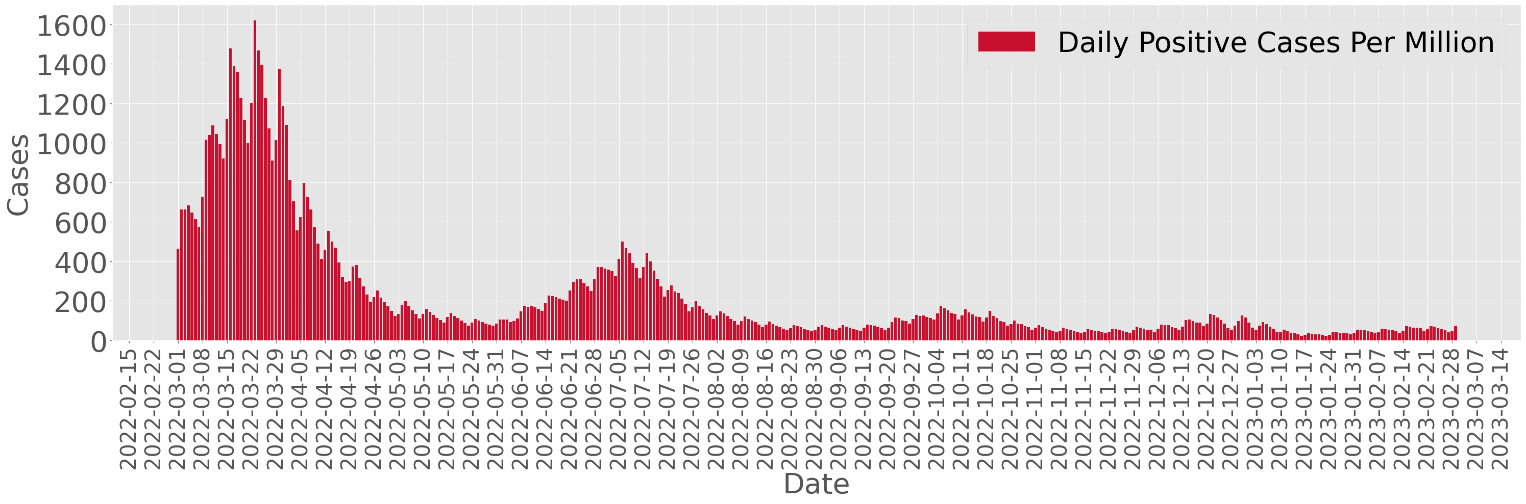
Figure 1: The daily infected cases in the United Kingdom from $03-01-2022$ to $02-28-2023$ (Mathieu et al., 2020).

It is common to record the number of infected cases on a daily basis. Based on the data format, we use $I(t)$ to represent the number of daily infected cases on day $t$, $t\in\mathbb{N}$. Then, the sampling interval is one day, i.e., $\eta=1$. Furthermore, the difference in the logarithms of consecutive daily infected cases is given by $\Delta_{\eta}(t)=\log(I(t))-\log(I(t-1))$, $t\in\mathbb{N}$. For instance, $\Delta_{\eta}(1)$ on $03-02-2022$ is obtained through differencing the infected cases on $03-02-2022$ and $03-01-2022$. Based on this formulation, we plot $\Delta_{\eta}(t)$ from $03-02-2022$ to $02-20-2023$ in Figure 2. Comparing Figure 2 to Figure 1, the difference $\Delta_{\eta}(t)=\log(I(t))-\log(I(t-1))$ can capture the spread trend. For instance, when $\Delta_{\eta}(t)$ is less than $0$ from $03-22-2022$ to $05-24-2022$ in Figure 2, the trend of the number of infected cases decreases in Figure 1. Conversely, when $\Delta_{\eta}(t)$ is greater than 0 from $05-31-2022$ to $07-05-2022$ in Figure 2, the trend of the number of infected cases increases in Figure 1. This observation aligns with Remark 2 such that when $\Delta_{\eta}(t)$ is greater than $0$, the daily infected cases are increasing, and when $\Delta_{\eta}(t)$ is less than $0$, the daily infected cases are decreasing. A value of $\Delta_{\eta}(t)=0$ represents the peak of a wave (i.e., a maximum) or the bottom of a valley (i.e., a minimum) in the daily spread. Additionally, the larger the value of $\left|\Delta(t)\right|$ is, the greater the change in daily infected cases between two consecutive days.

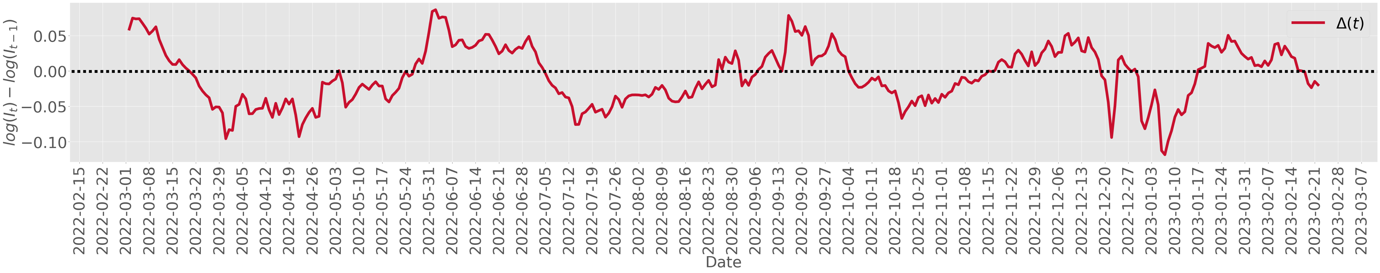
Figure 2: The difference in the logarithm of consecutive daily infected cases from $03-02-2022$ to $02-20-2023$.

We use Gaussian Process Regression to model $\Delta_{\eta}(t)$, $t\in\underline{n}$, where $n=356$ is the number of the days covering the period of interest from $03-02-2022$ to $02-20-2023$. Therefore, the training locations are $\{1,2,\dots,n\}$, and the corresponding training data are $[\Delta_{\eta}(1),\Delta_{\eta}(2),\dots,\Delta_{\eta}(n)]$, as shown in Figure 2. By applying the Gaussian Process Regression algorithm provided in Proposition 3.2, we visualize the model at the training time steps in Figure 3. The red solid line in Figure 3 represents the training data $\Delta_{\eta}(t)$, $t\in\underline{n}$. The blue dotted line illustrates the prediction mean, denoted as $m^{*}(t)$, at the training locations $t\in\underline{n}$. The shaded blue area, bounded by the blue dashed lines, indicates the $95\%$ confidence interval of the Gaussian Process Regression model. It is observed that when $\Delta_{\eta}(t)$ exhibits less fluctuation, the confidence interval becomes tighter. For instance, a comparison between the bounds from $10-25-2022$ to $11-08-2022$ and from $12-13-2022$ to $12-27-2022$ reveals a much tighter bound in the latter period.

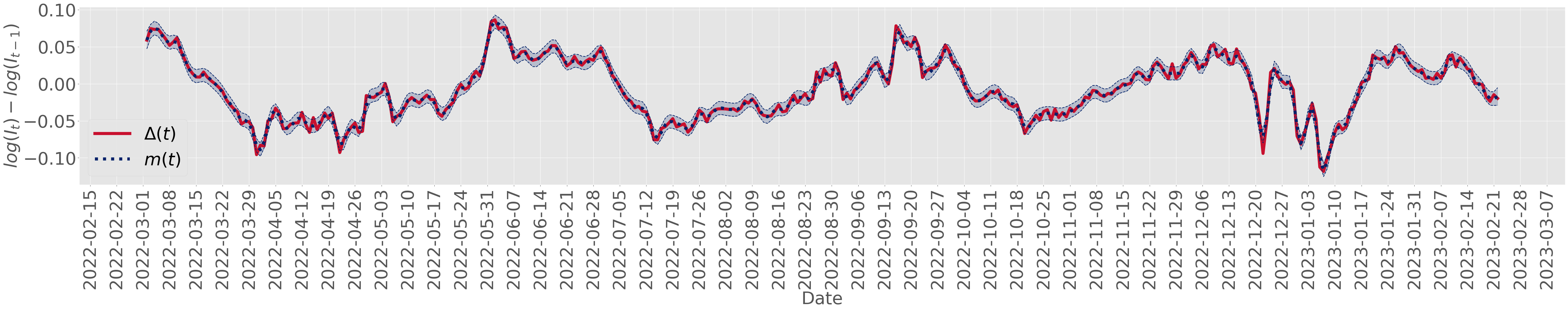
Figure 3: Gaussian Process Regression for $\Delta_{\eta}(t)$, $t\in\underline{n}$.

We employ Gaussian Process Regression to predict the spread in the near future. Consider $\Delta_{\eta}(t)$, $t\in\underline{h}$, where $h\in\mathbb{N}_{>0}$ and $h<n$. We use the data $[\Delta_{\eta}(1),\dots,\Delta_{\eta}(h)]$ to predict the data for the next seven days, denoted by $[m(h+1),\dots,m(h+7)]$. Specifically, we use data from $03-02-2022$ to the first day of each subsequent month (until $02-01-2023$) to predict the data for the next $7$ days after that first day. For instance, when using data from $03-02-2022$ to $12-01-2022$ to train the model, we make predictions from $12-02-2022$ to $12-08-2022$.

Figure 4 illustrates predictions for eleven one-week intervals. The red solid line represents the data $\Delta_{\eta}(t)$, $t\in\underline{n}$. The solid lines in the color palette style represent the predictions. For example, when predicting the spread from $12-02-2022$ to $12-08-2022$, we use all data from $03-02-2022$ to $12-01-2022$ to train the Gaussian Process Regression model. Similar to Figure 3, the dotted lines and the shaded area bounded by the dotted lines with the same color capture the $95\%$ confidence interval of the prediction.

Figure 4 shows that out of the 77 prediction points, 5 points at the testing locations are outside the $95\%$ confidence interval, resulting in a $93.5\%$ prediction accuracy based on the confidence interval. Among these 5 prediction points, 4 are during the first prediction interval from $04-02-2022$ to $04-08-2022$. We attribute the inaccurate prediction to the nearly monotonically decreasing trend in the training data, whereas there is a significant change in the trend starting from the prediction point on $04-02-2022$. However, we can still observe the turning point in the first prediction, even though we do not have the changing trend in the training data.

Furthermore, in Figure 4, for every prediction interval, we observe that the confidence interval grows as the time steps move from $1$ to $7$ steps away from the last time step of our training data points. This observation reflects that a longer prediction horizon will generate a larger prediction error. Figure 4 also illustrates that the prediction error will be higher if the function $\Delta_{\eta}(t)$ changes drastically within the time interval for regression, since a drastic change in $\Delta_{\eta}(t)$ will result in a higher Lipschitz constant $L_{\Delta}$ during that time interval. Comparing Prediction 1 and Prediction 8, where $\Delta_{\eta}(t)$ changes drastically during the time interval of the Prediction 1, we see less accurate predictions during the period corresponding to Prediction 1. As shown by this example, the spreading properties, the selection of the prediction horizon, and the infection data will impact our Gaussian Process Regression result.

5 Conclusion

In this work, we propose a novel approach to investigate the epidemic spreading process. Leveraging Gaussian Processes Regression, we model and predict the spread through the differences in the logarithm of infected data. Additionally, we provide an upper bound on the prediction variance and the prediction error, indicating the connection between the spread, prediction horizon, infection data, and the prediction error bound. In future work, we plan to leverage the model and prediction mechanism to design a new data-driven predictive control strategy for the epidemic mitigation problem.

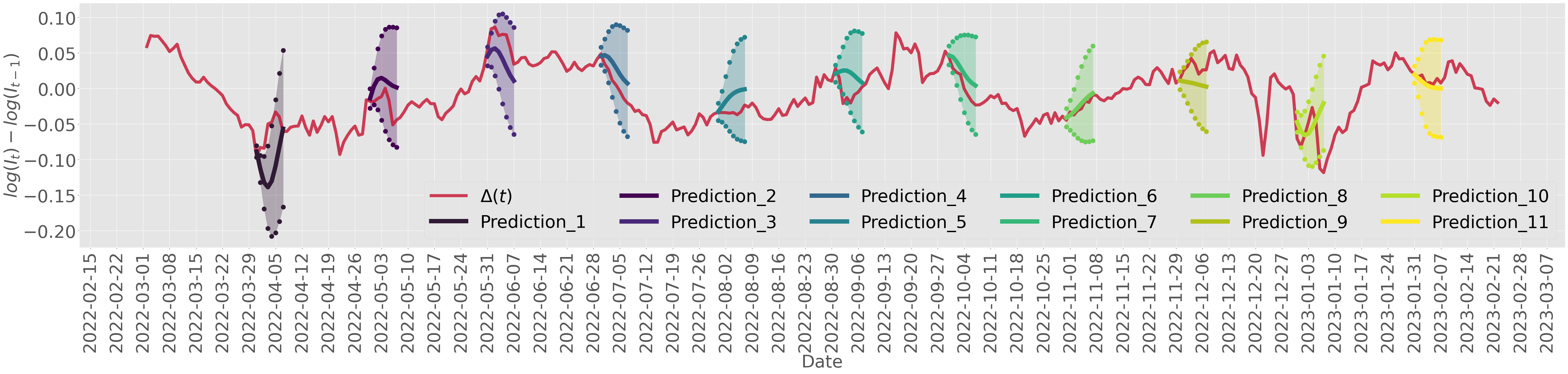
Figure 4: Gaussian Process Regression for epidemic spread prediction.

References

- Abbott et al. (2020) Sam Abbott, Joel Hellewell, Robin N Thompson, Katharine Sherratt, Hamish P Gibbs, Nikos I Bosse, James D Munday, Sophie Meakin, Emma L Doughty, June Young Chun, et al. Estimating the time-varying reproduction number of SARS-CoV-2 using national and subnational case counts. Wellcome Open Research, 5(112):112, 2020.
- Alazab et al. (2020) Moutaz Alazab, Albara Awajan, Abdelwadood Mesleh, Ajith Abraham, Vansh Jatana, and Salah Alhyari. COVID-19 prediction and detection using deep learning. International Journal of Computer Information Systems and Industrial Management Applications, 12(June):168–181, 2020.
- Alsayed et al. (2020) Abdallah Alsayed, Hayder Sadir, Raja Kamil, and Hasan Sari. Prediction of epidemic peak and infected cases for COVID-19 disease in Malaysia, 2020. International Journal of Environmental Research and Public Health, 17(11):4076, 2020.
- Anastassopoulou et al. (2020) Cleo Anastassopoulou, Lucia Russo, Athanasios Tsakris, and Constantinos Siettos. Data-based analysis, modelling and forecasting of the COVID-19 outbreak. PloS one, 15(3):e0230405, 2020.
- Casella (2020) Francesco Casella. Can the COVID-19 epidemic be controlled on the basis of daily test reports? IEEE Control Systems Letters, 5(3):1079–1084, 2020.
- Cori et al. (2013) Anne Cori, Neil M Ferguson, Christophe Fraser, and Simon Cauchemez. A new framework and software to estimate time-varying reproduction numbers during epidemics. American Journal of Epidemiology, 178(9):1505–1512, 2013.
- Datilo et al. (2019) Philemon Manliura Datilo, Zuhaimy Ismail, and Jayeola Dare. A review of epidemic forecasting using artificial neural networks. Epidemiology and Health System Journal, 6(3):132–143, 2019.
- Gallo Marin et al. (2021) Benjamin Gallo Marin, Ghazal Aghagoli, Katya Lavine, Lanbo Yang, Emily J Siff, Silvia S Chiang, Thais P Salazar-Mather, Luba Dumenco, Michael C Savaria, Su N Aung, et al. Predictors of COVID-19 severity: A literature review. Reviews in Medical Virology, 31(1):1–10, 2021.
- Genton (2001) Marc G Genton. Classes of kernels for machine learning: A statistics perspective. Journal of Machine Learning Research, 2(Dec):299–312, 2001.
- Gershgorin (1931) S Gershgorin. Uber die abgrenzung der eigenwerte einer matrix. lzv. Akad. Nauk. USSR. Otd. Fiz-Mat. Nauk, 7(6):749–754, 1931.
- Giordano et al. (2020) Giulia Giordano, Franco Blanchini, Raffaele Bruno, Patrizio Colaneri, Alessandro Di Filippo, Angela Di Matteo, and Marta Colaneri. Modelling the COVID-19 epidemic and implementation of population-wide interventions in Italy. Nature Medicine, 26(6):855–860, 2020.
- Hewing et al. (2020) Lukas Hewing, Kim P Wabersich, Marcel Menner, and Melanie N Zeilinger. Learning-based model predictive control: Toward safe learning in control. Annual Review of Control, Robotics, and Autonomous Systems, 3:269–296, 2020.
- Ketu and Mishra (2021) Shwet Ketu and Pramod Kumar Mishra. Enhanced Gaussian process regression-based forecasting model for COVID-19 outbreak and significance of iot for its detection. Applied Intelligence, 51:1492–1512, 2021.
- Khajanchi and Sarkar (2020) Subhas Khajanchi and Kankan Sarkar. Forecasting the daily and cumulative number of cases for the COVID-19 pandemic in India. Chaos: An Interdisciplinary Journal of Nonlinear Science, 30(7), 2020.
- Lederer et al. (2019) Armin Lederer, Jonas Umlauft, and Sandra Hirche. Uniform error bounds for Gaussian process regression with application to safe control. Advances in Neural Information Processing Systems, 32, 2019.
- Lederer et al. (2021) Armin Lederer, Jonas Umlauft, and Sandra Hirche. Uniform error and posterior variance bounds for Gaussian process regression with application to safe control. arXiv preprint arXiv:2101.05328, 2021.
- Maciejowski and Huzmezan (2007) Jan M Maciejowski and Mihai Huzmezan. Predictive control. In Robust Flight Control: A Design Challenge, pages 125–134. Springer, 2007.
- Mathieu et al. (2020) Edouard Mathieu, Hannah Ritchie, Lucas Rodés-Guirao, Cameron Appel, Charlie Giattino, Joe Hasell, Bobbie Macdonald, Saloni Dattani, Diana Beltekian, Esteban Ortiz-Ospina, and Max Roser. Coronavirus pandemic (COVID-19). Our World in Data, 2020. https://ourworldindata.org/coronavirus.
- Merow and Urban (2020) Cory Merow and Mark C Urban. Seasonality and uncertainty in global COVID-19 growth rates. Proceedings of the National Academy of Sciences, 117(44):27456–27464, 2020.
- Rahimi et al. (2021) Iman Rahimi, Fang Chen, and Amir H Gandomi. A review on COVID-19 forecasting models. Neural Computing and Applications, pages 1–11, 2021.
- Roda et al. (2020) Weston C Roda, Marie B Varughese, Donglin Han, and Michael Y Li. Why is it difficult to accurately predict the COVID-19 epidemic? Infectious Disease Modelling, 5:271–281, 2020.
- Sam Abbott et al. (2020) Sam Abbott, Joel Hellewell, Katharine Sherratt, Katelyn Gostic, Joe Hickson, Hamada S. Badr, Michael DeWitt, Robin Thompson, EpiForecasts, and Sebastian Funk. EpiNow2: Estimate Real-Time Case Counts and Time-Varying Epidemiological Parameters, 2020.
- Senanayake et al. (2016) Ransalu Senanayake, Simon O’Callaghan, and Fabio Ramos. Predicting spatio-temporal propagation of seasonal influenza using variational Gaussian process regression. In Proceedings of the AAAI Conference on Artificial Intelligence, volume 30, 2016.
- She et al. (2022a) Baike She, Shreyas Sundaram, and Philip E Paré. A learning-based model predictive control framework for real-time SIR epidemic mitigation. In Proceedings of the 2022 American Control Conference (ACC), pages 2565–2570. IEEE, 2022a.
- She et al. (2022b) Baike She, Shreyas Sundaram, and Philip E Paré. Optimal mitigation of SIR epidemics under model uncertainty. In Proceedings of the 2022 IEEE 61st Conference on Decision and Control (CDC), pages 4333–4338. IEEE, 2022b.
- Srinivas et al. (2012) Niranjan Srinivas, Andreas Krause, Sham M Kakade, and Matthias W Seeger. Information-theoretic regret bounds for Gaussian process optimization in the bandit setting. IEEE Transactions on Information Theory, 58(5):3250–3265, 2012.
- Talkhi et al. (2021) Nasrin Talkhi, Narges Akhavan Fatemi, Zahra Ataei, and Mehdi Jabbari Nooghabi. Modeling and forecasting number of confirmed and death caused COVID-19 in Iran: A comparison of time series forecasting methods. Biomedical Signal Processing and Control, 66:102494, 2021.
- van den Driessche (2017) Pauline van den Driessche. Reproduction numbers of infectious disease models. Infectious Disease Modeling, 2(3):288–303, 2017.
- Velásquez and Lara (2020) Ricardo Manuel Arias Velásquez and Jennifer Vanessa Mejia Lara. Forecast and evaluation of COVID-19 spreading in USA with reduced-space Gaussian process regression. Chaos, Solitons & Fractals, 136:109924, 2020.
- Wang et al. (2019) Lijing Wang, Jiangzhuo Chen, and Madhav Marathe. DEFSI: Deep learning based epidemic forecasting with synthetic information. In Proceedings of the AAAI conference on artificial intelligence, volume 33, pages 9607–9612, 2019.
- Wilke and Bergstrom (2020) Claus O Wilke and Carl T Bergstrom. Predicting an epidemic trajectory is difficult. Proceedings of the National Academy of Sciences, 117(46):28549–28551, 2020.
- Williams and Rasmussen (2006) Christopher KI Williams and Carl Edward Rasmussen. Gaussian Processes For Machine Learning, volume 2. MIT press Cambridge, MA, 2006.
- Woolhouse (2011) Mark Woolhouse. How to make predictions about future infectious disease risks. Philosophical Transactions of the Royal Society B: Biological Sciences, 366(1573):2045–2054, 2011.
- Wu et al. (2020) Yu Wu, Wenzhan Jing, Jue Liu, Qiuyue Ma, Jie Yuan, Yaping Wang, Min Du, and Min Liu. Effects of temperature and humidity on the daily new cases and new deaths of COVID-19 in 166 countries. Science of the Total Environment, 729:139051, 2020.
- Wu et al. (2018) Yuexin Wu, Yiming Yang, Hiroshi Nishiura, and Masaya Saitoh. Deep learning for epidemiological predictions. In Proceedings of the 41st International ACM SIGIR Conference on Research & Development in Information Retrieval, pages 1085–1088, 2018.
- Wynants et al. (2020) Laure Wynants, Ben Van Calster, Gary S Collins, Richard D Riley, Georg Heinze, Ewoud Schuit, Elena Albu, Banafsheh Arshi, Vanesa Bellou, Marc MJ Bonten, et al. Prediction models for diagnosis and prognosis of Covid-19: Systematic review and critical appraisal. The BMJ, 369, 2020.