package/before/amsmath
Residual U-net with Self-Attention Network for Multi-Agent Time-Consistent Optimal Trade Execution
Abstract
In this paper, we explore the use of a deep residual U-net with self-attention to solve the the continuous time time-consistent mean variance optimal trade execution problem for multiple agents and assets. Given a finite horizon we formulate the time-consistent mean-variance optimal trade execution problem following the Almgren-Chriss model as a Hamilton-Jacobi-Bellman (HJB) equation. The HJB formulation is known to have a viscosity solution to the unknown value function. We reformulate the HJB to a backward stochastic differential equation (BSDE) to extend the problem to multiple agents and assets. We utilize a residual U-net with self-attention to numerically approximate the value function for multiple agents and assets which can be used to determine the time-consistent optimal control. In this paper, we show that the proposed neural network approach overcomes the limitations of finite difference methods. We validate our results and study parameter sensitivity. With our framework we study how an agent with significant price impact interacts with an agent without any price impact and the optimal strategies used by both types of agents. We also study the performance of multiple sellers and buyers and how they compare to a holding strategy under different economic conditions.
Keywords T
ime-consistent Mean Variance; Optimal Trade Execution; Portfolio Management; Deep Neural Networks; Multi Agent Games; Reinforcement Learning, Convolutional Neural Networks
1 Introduction
The optimal trade execution model was developed as a framework that would allow traders to control the speed of their portfolio liquidation in order to limit the disadvantages of liquidating an asset too quickly or too slowly Almgren and Chriss [2000]. This is done to limit the fluctuation of prices due to large volume movements. However, the framework for optimal trade execution under the mean variance criteria is time inconsistent due to the variance term which is non-monotonic with respect to wealth Basak and Chabakauri [2010]. If the optimal control given at time is time-inconsistent then it does not mean that the control will remain optimal at a later time . Thus, the optimal portfolio execution problem is usually solved for time and the portfolio is not changed until the portfolio matures at . This strategy is referred to as the pre-commitment strategy.
The pre-commitment solution to the mean-variance problem often reformulates the original mean-variance problem to an equivalent formulation Li and Ng [2000]; Forsyth [2011]; Bjork et al. [2017]. Pre-commitment strategy works well within stable economic regimes and is shown to outperform time-consistent strategies Forsyth [2020]; Vigna [2020]. However, the pre-commitment assumes that there is complete information from to but in reality the state of the economy might change drastically within a given time period due to exogenous factors. The absence of time consistency also prevents us from using dynamic programming directly.
To overcome the time inconsistency problem of the mean variance criteria, there has been increasing development in continuous time consistent mean variance asset allocation in both reinsurance and investments Guan and Hu [2022]. The current approaches typically solve the continuous time optimal portfolio allocation problem Zhou and Li [2000]; Aivaliotis and Veretennikov [2018]; Aivaliotis and Palczewski [2014]; Wang and Forsyth [2011]. The approach in Van Staden et al. [2018] considers the control of impulse controls in jump processes.
In discrete time, this problem has been solved using dynamic programming assuming local optimality Basak and Chabakauri [2010]. The discrete time solution does not solve for the value function of the Hamilton-Jacobi-Bellman (HJB) equation. The analytical solution to the continuous time consistent mean variance asset allocation problem has been studied for an agent with -assets Zhou and Li [2000] and in the asset reinsurance and investment setting using agents Guan and Hu [2022]. Note, the optimal asset allocation problem can be viewed as a special case of the optimal trade execution problem when there is no price impact, i.e. and for agents who can only sell/buy the asset. The numerical solutions to the optimal trade execution problem has been presented for the time-inconsistent strategy using finite difference methods (FDM) Forsyth [2011]; Wang and Forsyth [2011]. The FDM solution to the time-consistent mean variance asset allocation problem, i.e. control on , and its extension to impulse control has also been solved Van Staden et al. [2018].
Recent advances in reinforcement learning (RL) uses model free methods to solve the optimal trade execution on limit-order-books and real data Ning et al. [2021]; Lin and Beling [2021]; Chen et al. [2022]. A RL framework that solves the continuous time mean-variance portfolio optimization problem derives the optimal policy iteration Wang and Zhou [2020]. However, this only considers the control of the portfolio allocation and not the optimal trade rate. A RL method has been used to approximate the optimal trade execution under mean variance criteria in the discrete time setting Hendricks and Wilcox [2014]. Typically, RL methods use the model free (Q-learning) approach. However, the issue with using Q-learning in the optimal trade execution in discrete time is that the problem is solved locally and does not guarantee the solution given satisfies the HJB equation Basak and Chabakauri [2010]. In current frameworks, there is no clear environment where agents can interact with. The agents learn independently based on a general simulated market. In this paper, we propose a multi-agent model which couples each agent implicitly through the price of the asset. This creates an environment that takes into account the decisions made by each individual agent and allows us to simulate the market dynamics more precisely.
In addition, none of the existing numerical solutions has formally addressed the problem of solving the time-consistent mean variance optimal trade execution problem in continuous time for higher dimensions. The analytical solutions are restricted to the control on the portfolio allocation, , and cannot be extended to the control of the trade rate, , because the trade rate is a non-linear control. This motivates the need for numerical solutions to the continuous time time-consistent mean variance optimal trade execution problems in higher dimensions.
In this paper, we extend the optimal trade execution formulation to the time-consistent framework and the use of neural networks to solve the high-dimensional optimal trade execution problem for assets and agents. The contributions of this paper are summarized as follows:
-
1.
We present a time-consistent optimal trade execution framework for multiple assets and multiple agents. This framework allows us to couple multiple agents through the stochastic stock price process indirectly using price impact, and to create an environment where multiple agents can interact with.
-
2.
We formulate the mean variance optimal trade execution problem such that the investor is aware of other investors in the market. We reformulate the mean variance problem into its dual representation and an auxillary HJB equation. To extend this framework into higher dimensions, we reformulate the HJB equation as a backward stochastic differential equation (BSDE). The auxillary HJB equation has been shown to have a viscosity solution Aivaliotis and Veretennikov [2018].
-
3.
We present a neural network solution for the -dimensional assets and -agent optimal trade execution problem using neural networks, which extends the numerical solution of the time consistent optimal trade execution problem to high dimensions. We use techniques based on neural network pricing of high dimensional options to formulate a deep residual self-attention network that overcomes the need to save weights at each timestep E et al. [2017]; Chen and Wan [2021]; Han and E [2016]; Hure et al. [2020].
-
4.
We show numerical experiments on the interactions of -agent optimal trade execution under different market conditions in a finite horizon setting.
In Section 2, we describe the optimal trade execution problem and extend it to the -dimensional setting. The extension of the optimal trade execution to agents with agents that are aware of the relative performance of other agents. In Section 3, we formulate at the HJB PDE representation of the -dimensional, agent optimal trade execution problem, its equivalent BSDE formulation and its approximate discretization. In Section 4, we discretize the BSDE to the least squares problem and introduce the neural network models used to solve them. In Section 5, we present numerical results and conclude in Section 6.
2 Mean-Variance Optimal Trade Execution
In this section, we present the optimal trade execution problem with assets and -agents. This is an extension of the classical framework Forsyth [2011]. Suppose each agent , where , can observe a basket of stocks in the market; with price process . Then the number of shares of the stocks owned by agent is given by and the amount invested in a risk free bank account is given by . Let be the time up to maturity , then at any time , the market agent has a wealth given by:
| (1) |
To handle buying and selling cases symmetrically, we start off with in cash, shares if we are selling and shares if buying. This means that we are trying to liquidate a long (short) position if we are selling (buying). More precisely
| (2) | ||||
| (3) |
where is the cash generated by selling/buying in . The objective is to maximize the wealth at maturity, , and simultaneously minimize the risk as measured by the variance. Note that due to the non-monotonicity of the variance term, this problem as presented is time inconsistent Basak and Chabakauri [2010]; Tse [2012].
A natural optimization criteria to consider for optimal trade execution is the mean variance (MV) strategy of Markowitz. The MV strategy looks for the optimal strategy that maximizes an investors expected gain, and at the same time minimizes their risk Wang and Forsyth [2011].
In this section we define the mean-variance criteria for optimal trade execution. The agent with trade rate maximizes the expected wealth defined as and minimizes the variance defined as
This can be reduced to a single cost function given by
| (4) |
where is the risk preference of the investor . Then the mean-variance optimal execution problem is to determine the strategy such that:
| (5) |
Let be the optimal control that maximizes (5), then the optimal cost function is given by
In general, the solution for the mean-variance problem is time inconsistent. Many approaches have been explored to overcome this limitation by solving an auxiliary problem which is referred to as the time-consistent mean variance problem Zhou and Li [2000]; Forsyth [2011]; Tse [2012]; Aivaliotis and Palczewski [2014]; Van Staden et al. [2018]; Forsyth [2020]; Guan and Hu [2022].
2.1 Problem Formulation
The dynamics of the optimal trade execution problem can be formulated by the Almgren-Chriss model Almgren and Chriss [2000]. The instantaneous trade rate is given by:
where is the amount of stock held by a liquidating agent. Let be the drift, be the risk free rate and be the volatility of the asset. The price process of the risky asset follows the Geometric Brownian motion (GBM) Forsyth [2011]:
where is the level of permanent price impact. The cash position is then given by Forsyth [2011]:
where is the level of temporary price impact. We can define the temporary price change due to the temporary impact as , .
Given states at the instant before the end of the trading horizon, we have one final liquidation (if ) to ensure that the number of shares . The liquidation value is computed as follows Tse [2012]:
2.2 Extension of the Almgren-Chriss model to Assets and agents
In this section, we describe how we extend the dynamics of the optimal trade execution problem to assets and agents. First, we consider assets and one agent. Let the trade rate for each asset be given by:
| (6) |
we can define the the aggregate trade rate for an agent as . As with the one dimensional case, we assume the process follows the GBM, with a modification due to the permanent price impact. Let and be the drift and volatility of stocks . Let be the correlation matrix and we define the correlated random variable , where are i.i.d, and is the Cholesky factor of , i.e. .
Given a vector of initial prices, , for each asset , we have:
| (7) |
with initial condition .
For simplicity, we assume that the market has sufficient liquidity and we do not consider market frictions. A multi-asset optimal trade execution problem has been modelled by a Orstein-Uhlenbeck (OU) process Bergault et al. [2022]. In our model, we assume a constant , and and we introduce a permanent price impact function in (7). We use the following linear form for the permanent price impact
where the constant is the permanent price impact factor. A linear permanent price impact function is used to eliminate round-trip arbitrage opportunities Tse [2012].
Given a stock price , The bank account is assumed to follow
| (8) |
where is the temporary price impact of the investor as they sell/buy the asset . The function is assumed to have the form
where is the bid-ask spread for each asset , is the temporary price impact factor of the investor and is the price impact exponent Forsyth [2011].
Next, we extend the optimal trade execution problem to -agents. Let , then the trading rate for each agent and each asset is given by
| (9) |
and the aggregate trade rate for each agent is given by:
Formally, we introduce the trade impacts in the price of asset as
where . This couples the actions of each agent implicitly through the price dynamics. Note, since our economy or state space is modeled through the asset prices, it is a way for each agent’s actions to update the state space. This also means the economy has full information about each agent . In this formulation, the trade rate of each trader affects other traders through the permanent price impact on each asset . This tells us that the asset price is driven by not just the drift of our asset but also by the accumulation of permanent price impact of each agent . This is consistent with the observation that in a multiple agent setting the total market impact on an asset is the sum of permanent price impact of all agents and the temporary price impact Schoneborn [2008].
The cash dynamic for each agent is given by
where
The temporary price impact factors of each agent only affects the execution price of agent , thus there is no coupling involved in this term with other agents. This gives us a measure of how each agent perceives their own impact on the market.
2.3 Mean Variance Criteria of Performance Aware Agents
We can extend our framework to consider agents that are aware about their performance relative to others. We refer to these agents as performance conscious agents of degree . More formally, for agent , let the market average wealth be given by Guan and Hu [2022]:
Then for we let and the mean-variance criteria becomes Guan and Hu [2022]:
| (10) |
where is the risk aversion parameter of each agent . Note that by setting in (10), the cost function reduces to (4). The solution to the -agent problem results in an optimal control Guan and Hu [2022]. The Nash equilibrium has been shown in Guan and Hu [2022] and is given by the following definition:
Definition 2.1.
Optimal control of time consistent mean-variance problem for -agents Guan and Hu [2022]. Let be the admissible control . A vector is said to be a time-consistent optimal strategy, any fixed initial state and a fixed number , a new vector defined by:
satisfies:
for . In addition, the optimal value function is defined as:
Remark 1.
The time-consistent solution satisfies the conditions of a subgame perfect Nash equilibrium Van Staden et al. [2018]. We remark that in this paper, we use the term optimal control instead of equilibrium control in order to be consistent with other numerical approaches in the literature Van Staden et al. [2018]; Wang and Forsyth [2011]; Bjork et al. [2017] .
3 Backward Stochastic Differential Equation (BSDE) Representation of the HJB Equation
In this section, we present the optimal trade execution problem using an auxiliary HJB formulation and its BSDE. The HJB formulation has been shown to have a viscosity solution Aivaliotis and Veretennikov [2018]. We also show that when there is no price impact, the formulation reduces to the optimal investment problem. We reformulate the HJB to the BSDE in order to solve the optimal trade execution problem as a stochastic optimization problem which is more suitable for applications of neural networks.
3.1 HJB Formulation
We derive the general HJB equation for a performance conscious agent . We first look at the HJB equation for a single agent with a single asset. To simplify the exposition, we drop the dependence on when it is clear. We define the value function such that:
The value function can be solved by reformulating the problem as an auxiliary problem Wang and Forsyth [2011]. However, the auxiliary problems do not permit a viscosity solution. To overcome this, we can rewrite the variance term such that Aivaliotis and Veretennikov [2018]:
Then the original mean-variance criteria becomes:
| (11) |
where is the value function of the Markovian control problem given by Aivaliotis and Veretennikov [2018]:
| (12) |
Note that solves (11). Let . Then the HJB equation that solves (12) is given by:
| (13) |
with terminal condition
We extend this formulation to a performance conscious agent Guan and Hu [2022] by replacing with . We formally extend (13) to agents and assets in the following Lemma:
Lemma 3.1.
For each agent with assets , the extended HJB equation is given by:
| (14) |
Proof.
Let , where and . Let be the timestep size, , and , then by the optimality of the control and law of iterated expectation for each the value function of the auxiliary problem is given by:
| (15) |
Let , then (15) can be written as
| (16) |
Applying Ito’s Lemma on , we get:
where
The expectations of and are straight forward. The expectation of requires more thought. Applying Ito’s lemma on , the expected value is given by:
Expanding (16) and evaluating gives us:
where
Diving out the and bringing the supremum inside the expectation gives us the extended HJB equation. ∎
Remark 2.
Special Case:
For the special case of , i.e. there is no price impact, the optimal trade execution reduces to the optimal asset allocation problem. The analytical solution to the optimal asset allocation problem for time-consistent mean-variance problem is known and has been solved in the linear-quadratic (LQ) sense Zhou and Li [2000]; Li and Ng [2000].
3.2 BSDE Formulation
A stochastic approach has an advantage in that the HJB can be extended to include multiple assets and multiple agents. This is computationally infeasible with the PDE approach even with the dimensional reduction techniques Forsyth [2011]. This is because each PDE for variance and wealth requires a three dimensional grid even with one asset. Though dimensional reduction can be used, this is does not apply for the general performance conscious agent due to the averaging term. We drop the explicit dependence on to keep the notation concise. To solve (14), we formulate the BSDE for using the following lemma.
Lemma 3.2.
Proof.
The significance of the system of BSDEs is two fold. One, the system of BSDEs does not require us to compute the Hessian of the extended HJB equation. This a big advantage as it allows us to avoid computing the second derivative on since computation of the second derivative can be very costly for high dimensions. This reduces the computational complexity of the problem. The second significance of the system of BSDEs is that it allows us to solve (17) in a least squares sense which is a recent technique used in high-dimensional option pricing Han and E [2016]; E et al. [2017]; Hure et al. [2020]; Chen and Wan [2021]; Na and Wan [2023]. This allows us to avoid using numerical solutions to the PDE and overcome the issue with dimensionality. Note, we can replace in (11) and (12) with for the case where the agent is performance conscious, i.e. .
3.3 Discretization of BSDE
We use the Euler’s method to simulate the forward SDE (7) through time. Let be the indices of simulation paths and be the indices of the discrete time-steps from to . Let be the timestep size and let . We discretize as and (7) as:
| (18) |
for . Next we discretize the position in the bank account, , using (8):
| (19) |
The number of shares in stocks, , is updated using (9). Thus the discretized dynamics of is given by:
| (20) |
The total wealth for each agent at each timestep can be calculated as:
When , we need to account for the cash account at each timestep by:
Let be the space of bounded trade rates. Then is the discretization of into number of discrete points. Equations (18), (19), and (20) are simulated forward in time over a subset of discretized control values . The discrete set of control points does not need to be too dense and we restrict it to the discrete set shown in Forsyth [2011].
To discretize the system of BSDEs, we first let be the approximations of the partial derivatives with respect to , respectively, defined as follows:
Then we can discretize (17) as:
where
The recursive system of equations to solve for at time from is then given by:
We can approximate at timestep by:
and enforcing time-consistency through each discrete timestep the approximation of is given by:
| (21) |
Note that the BSDE (21) is solved backward in time.
3.3.1 Least squares formulation
To solve the BSDE (21), we approximate by and reformulate the problem in a least squares formulation. Consider the timestep from (21), the pointwise residual is given by:
The objective becomes the minimization of the residuals such that . This gives us the criteria we need to form the following least squares problem:
| (22) |
Minimizing (22) gives us a good approximation to . The optimal control can then be determined by:
4 Neural network approach to the optimal trade execution problem
In this section, we propose a neural network approach to solve the system of least squares formulation (22). The method follows a general framework that has been used to solve high-dimensional American option pricing problems and has shown to produce good results Han and E [2016]; E et al. [2017]; Hure et al. [2020]; Chen and Wan [2021]; Na and Wan [2023]. This framework has also been used to solve more general HJB equations as shown in Hure et al. [2020].
4.1 Neural network formulation
We model the approximations using a deep residual U-net with a self attention layer. U-net is a convolutional neural network architecture with great success in image processing and was first introduced for the application of biomedical image segmentation Ronneberger et al. [2015]. We chose this architecture to learn the relationship between the discretized trade rates and assets. This is because U-net has been shown to use and augment existing features more effectively Ronneberger et al. [2015]. We also explore the use of self-attention layer to increase the efficiency of the residual deep network by embedding temporal relationship between the previous estimate and the current states given by {, }. The use of a self-attention layer allows our network to determine which features are the most relevant in predicting the output Vaswani et al. [2017]. This allows us to avoid using recurrent network structures which have a chance to exhibit vanishing gradient properties due to the activation functions used in their gate structures Vaswani et al. [2017].
4.1.1 Self-attention residual network
The standard attention network was initially used to model predictive sequential language models Vaswani et al. [2017]. They were initially implemented to learn the importance of features in predicting a language sequence. The self-attention architecture was introduced as a method to embed information inputs to create latent feature space for more efficient training Vaswani et al. [2017]. In this paper, we use self-attention layer to overcome the limitation of deep residual network methods. Deep residual networks need to save weights at every timestep Han and E [2016]; E et al. [2017]; Chen and Wan [2021]; however, by adding the self-attention layer allows us to capture the dependencies between features.
The attention mechanism relies on a query , and key-value pair . We let be the score function given by Vaswani et al. [2017]:
where the softmax function is a standard activation function Goodfellow et al. [2016] and is the length of the sequence. Let be the number of heads where each head is given by . It was found that constructing multiple attention layers in a bagging approach allowed for better performance than a single attention mechanism Vaswani et al. [2017]. The multi-head attention mechanism is the concatenation of heads and is defined as Vaswani et al. [2017]:
where is used to signify concatenation. It has been shown that using a linear layer to represent is beneficial to learning Vaswani et al. [2017]. The self-attention network is a special case of the multi-head attention mechanism where the inputs are passed through a linear layer to construct . More specifically, given an input and weights , , we can define , , .
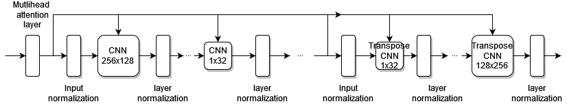
The self-attention mechanism itself does not have much prediction power Vaswani et al. [2017]. To add prediction power to the self-attention layer, we couple it with a convolution neural network (CNN). The benefit of using a CNN is that it captures the high dimensional structure across the discretized space of trade rates and our input features Goodfellow et al. [2016]. More specifically, we use a U-net architecture coupled with a residual structure. The U-net we use has convolution layers and transposed convolution layers with a converging-diverging geometry as shown in Figure 1 Ronneberger et al. [2015]. The convergent-divergent structure of the U-net allows for the network to capture the content in the data and allows for localization Ronneberger et al. [2015]. It also allows us to limit the effects of features that may not contribute to predictions.
In between each network layer, we normalize the input . Normalization allows our network to learn more effectively and prevent cross correlation between network layers Goodfellow et al. [2016]. For learnable parameters and to assist convergence of the deep residual network, we use group normalization, , given by He et al. [2016]:
where is some small number to aid in numerical stability.
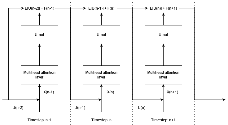
For a given input, , at timestep , the residual U-net for each timestep has the following form He et al. [2016]:
where is the weight of a linear layer. The residual U-net with self-attention used in this paper is shown in Figure 2. The network becomes a deep network as we unroll each network through time. By adding to the output, it gives our network a residual network structure through time.
To solve (21), we first approximate the function using the deep residual network with self attention. Given the set of weights , let be the neural network approximation to . The initial input is used to construct the self-attention mechanism , where each head is given by . The output is then added to the original input and normalized. More precisely, is given by:
This new input is then passed through our residual U-net. This allows us to learn spatial relationship between our features and the discretized trade rates.
In our network, we use the swish activation function over the ReLU activation function. This is because the ReLU activation function may cause information loss when training over long sequences due to the negative values being zeroed out Na and Wan [2023]. The output of CNN plus some weighted gives us the final output:
For timestep and sample , the neural network approximation to is given by:
Note that the number of time-steps represents the depth of the deep residual self-attention network.
4.2 Network Training and Prediction
Let be the deep self-attention residual network approximation of with parameters for agent . The parameters are the weights and biases of the deep self-attention residual network. The input data of is given by . We concatenate the output from the previous time-step into our input. This information is used by the self-attention mechanism to embed previous timestep information into the model. The last three inputs give positional data for time, simulation path, and control index on the discretized set of control points . The label data used to train the network is given by the value function from the previous timestep and is given by:
This is because the BSDE is solved backward in time and we must satisfy the terminal condition (12). We let
where
and let
We rewrite the losses (22) such that
Minimizing gives us the optimal set of parameters for the self-attention network given by:
We summarize the training of the proposed model in Algorithm 1. The gradients are computed using autodifferentiation.
To compute for agent we run an inference of the network. We perform a linear search for the optimal expected trade rate for each asset over the grid of . We summarize the inference step of the proposed model in Algorithm 2.
Note, due to the non-uniqueness of the optimal control, we train multiple networks for each agent and perform bagging to ensure better results. This allows our neural network to explore multiple paths. Optimization is done using the Adam algorithm Kingma and Ba [2017] with a learning rate of .
4.3 Data Generation
To construct the training data used by the deep residual self-attention network, we need to perform forward simulations for the dynamics of the underlying asset , cash position , position in stocks , and the control . At , we initialize the variables according the initial conditions given by (2) for the variables . The trade rate is constructed as a uniform grid of discretized points over points. The trade rate is given by:
where is in units of . For , the dynamics of (18) is simulated using Euler’s method. The dynamics of follow the dynamics given by (19) and (20). To ensure that all assets are liquidated at time , we define the trade rate, , at the instant before maturity as Forsyth [2011]:
The cash position is updated one final time at so as to penalize all positions that have not been liquidated at the final trading step. This is done at the end of the forward simulation in order to compute the value function at terminal time .
5 Numerical Results
In this section, we outline the numerical experiments to validate the proposed method. We demonstrate the effects of different parameters on the proposed method and the numerical studies on different strategies used in optimal trade execution.
In Experiment , we look at a special case when the trade impact factors to validate the proposed method. In Experiment we observe at the effects of different parameters on . In Experiment , we study the case of agents where one agent has a large permanent price impact trading in an environment while the other agent has no impact. In this setting, we also vary and consider the cases when the economic conditions are good and bad . In Experiment , we study the neural network solution to the optimal execution problem with agents on different strategies in different market conditions. We also look at the effects of correlation when agents are trading assets. In Experiment , we study the neural network solution with agents and assets. We divide the agents into buyers and sellers and demonstrate the performance of each group of liquidating agents and compare them to a strategy where they just hold the asset from .
All experiments are done using a 6GB-NVIDIA GTX 2060 GPU, a 6 core AMD Ryzen 5 3600X processor and 16GB of RAM.
5.1 Experiment 1: Comparison of Residual Attention Network to Existing solutions
In this experiment, we compare the approximation of the neural network solution to the results of existing work Forsyth [2011]; Aivaliotis and Veretennikov [2018]; Guan and Hu [2022]; Zhou and Li [2000]. This experiment verifies that the outputs of our neural network solution coincides with known solutions wherever they are available. We fix the parameter and assume no price impact, i.e. and .
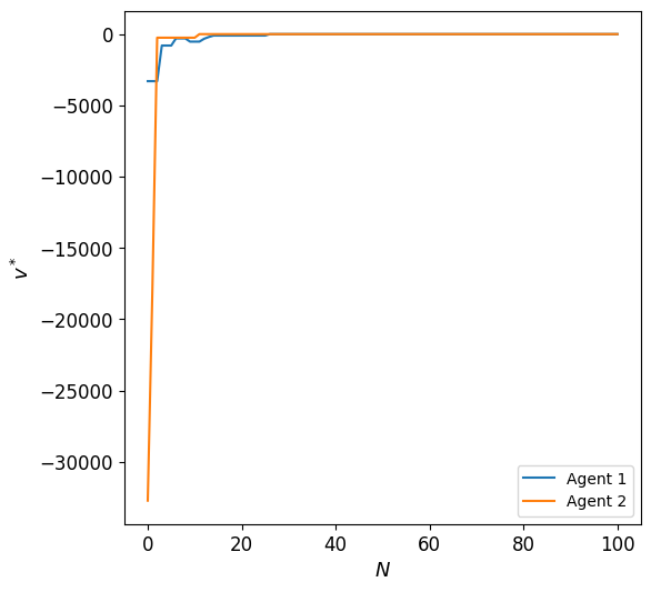
Single agent, single asset
In the case of a single agent with one asset, we compare the results to the FDM solution Forsyth [2011]; Aivaliotis and Palczewski [2014]. First, we look at the performance of the proposed method for different . This is done to determine the appropriate number of timesteps we need for an accurate solution to the problem. We fix , year and run the neural network until and summarize the results in Table 1. We also record the FDM solution for with relative error given by:
| (23) |
We treat the FDM solution as the actual solution and the NN solution is the approximation.
| FDM | Proposed method | Relative error | |
|---|---|---|---|
We see that the proposed method has the smallest relative error to the FDM solution at . We found that a network depth tends to over fit the data, which is shown by the decrease in accuracy.
Next, we show the sample size that minimizes the relative error. This is done to determine the appropriate batch size we need to accurately compute our results. We fix and run the neural network until convergence. The results are summarized in Table 2. In Table 2, we record the FDM solution for the number of space grids . We observe that the proposed method has the smallest relative error to the FDM solution at .
| FDM | Proposed method | Relative Error | |
|---|---|---|---|
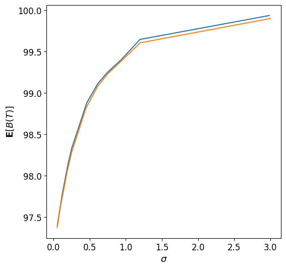
We also make a comparison to the FDM solution to the optimal trade execution for , , and Forsyth [2011]. We compute the efficient frontier Tse [2012] as shown in Figure 3. For an initial price of and , the expected gain from selling is with a standard deviation of Forsyth [2011]. Our neural network approximation gives an expected gain of with a standard deviation of , similar to the FDM results.
Single agent, assets
We compare the neural network solution with analytical solutions. For the special case of no price impact, an analytical solution exists for the case of a single agent with multiple assets Zhou and Li [2000]. This experiment shows that our outputs are consistent with multidimensional results.
Let be the vector of drift rates and the covariance matrix for each assets . Note this framework assumes independence between the assets, and hence we represent the volatilities as a vector. The time-consistent mean variance optimal asset allocation for multiple assets is given by Zhou and Li [2000]:
where parameter and . Let, , and let be the quantity of assets held by the agent. Then the optimal asset allocation for a single agent with multiple assets is given by Zhou and Li [2000]:
| (24) |
where Our model can be used to compute by solving the equation . We fix , and and compute using Monte Carlo simulation Zhou and Li [2000]. Given , the optimal value for at years are summarized in Table 3. We see that the highest relative error occurs at with a relative error of .
| Analytical Solution | Proposed method | Relative Error | |
|---|---|---|---|
agents, single asset
We compare the neural network solution with analytical solutions. For the special case of no price impact, an analytical solution exists for multiple agent with one asset Guan and Hu [2022]. The mean-variance optimal portfolio problem can be written as Guan and Hu [2022]:
The analytical solution to the time-consistent auxiliary problem is given by Guan and Hu [2022]:
| (25) |
We use Monte Carlo Simulation to compute Guan and Hu [2022]. Given the optimal value for are summarized in Table 4. We present results for only one agent as the agents are assumed to be symmetric. We can see from Table 4 that the relative errors are generally small with the highest relative error of occurred at .
| Analytical Solution | Proposed method | Relative Error | |
|---|---|---|---|
To summarize, the proposed model performs well in both multi-agent and multi-asset cases.
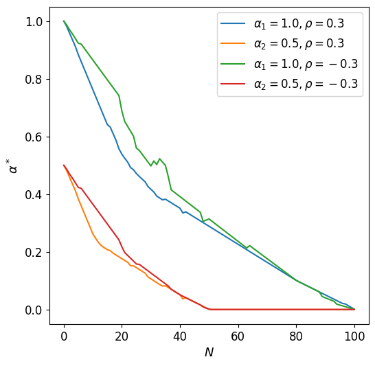
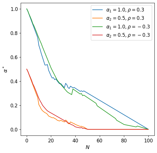
5.2 Experiment 2: Sensitivity of Parameters
In this experiment, we study the effects of the relative performance factor , the risk preference , the permanent price impact factor and the temporary price impact factor on the optimal portfolio . We vary each of these factors independently and observe the portfolio at different time-steps for agents with asset. For the sensitivity study we assume that agents want to liquidate long positions (sell only). We set , , , , , and .
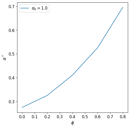
To analyze the sensitivity of , we let , and . The results are shown in Figure 4. As we can see, as increases, also increases. This is expected since the agent invests more into risky assets as they become more aware of other agents Guan and Hu [2022]. Thus our neural network approach is able to capture this behaviour correctly.

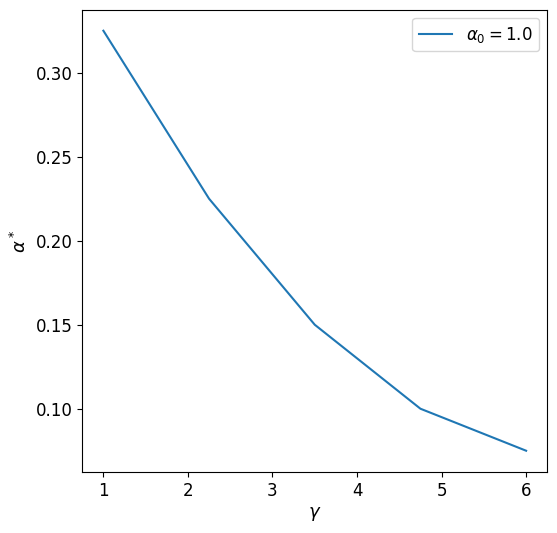
Moreover, we also want to ensure that decreases as increases. This behaviour is an important behaviour to observe in agents as it is commonly known that as the risk aversion increases, the agent invests less in risky assets Zhou and Li [2000]. We fix , , and . Figure 5 shows that indeed decreases as increases, illustrating the effectiveness of the neural network approach.
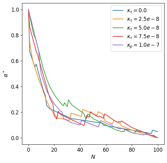
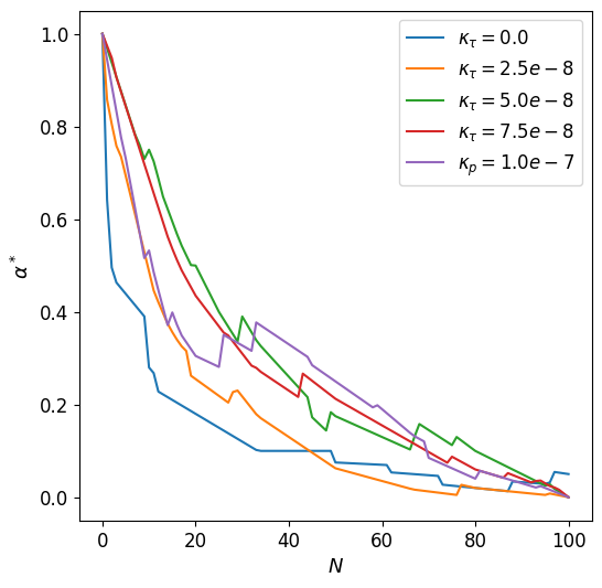
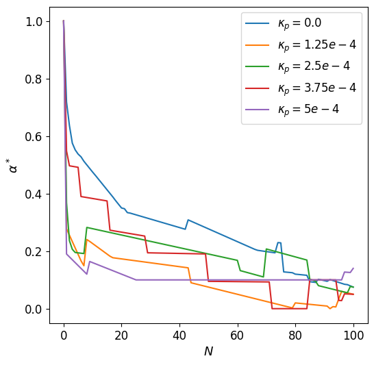
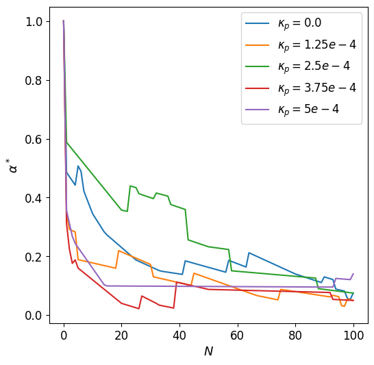
To observe the effects of and , we fix and . We choose to fix to avoid influence of other agents to the dynamics. In Figure 6, we plot over different time-steps for different (top) and (bottom) for both agents.
The temporary price impact, , is the local impact each agent has on the asset price due to the velocity of trade. To maximize the trade criteria, the agents take a less aggressive approach and prefer to liquid their positions in a more gradual manner. We observe that when the permanent price impact, , is low the agent trades more actively and the activity decreases as increases. This is expected because as the permanent price impact increases, the more impact the agent has on the asset price. Since the goal of the optimal execution problem is to trade the asset without affecting the price as much as possible the agent will be more hesitant to trade as their permanent price impact increases.
5.3 Experiment 3: Optimal Execution in Advantageous and Disadvantageous Market Conditions for Agents and the Effects of Correlation
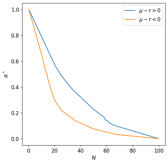
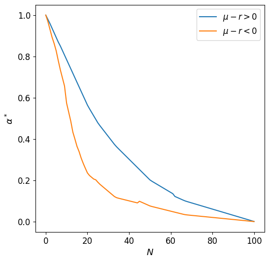
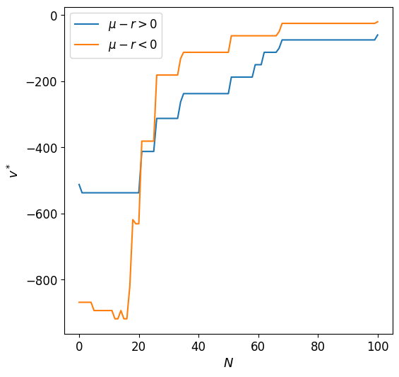
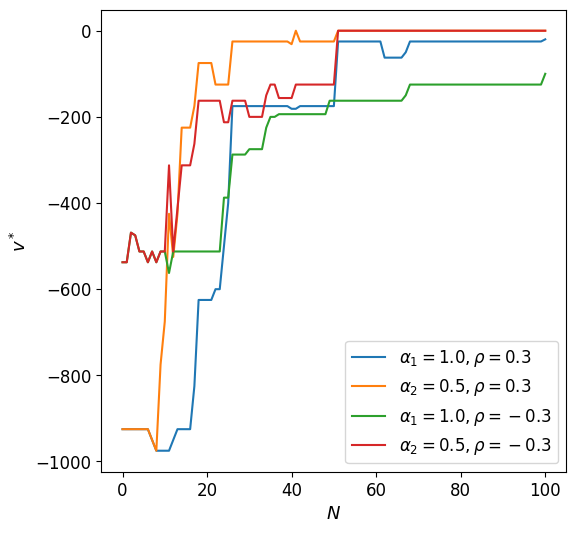
In this experiment, we study the affects of macroeconomic pressure on the asset. We consider , two agents that sell off asset and consider two cases. To simulate good market conditions, we set . In contrast, to simulate poor market conditions we set . We assume there is no permanent price impact, i.e. , and . For good market conditions, we set and . For poor market conditions, we set the . Figure 7 shows the sell only strategy of agent (left) and agent (right). The portfolio is presented in the top figures and the controls are presented in the bottom figures.
In Figure 7, we observe that the agents liquidate their position faster if they expect the price of the asset to decrease. This is expected but how they choose to sell is important to observe. We can see the optimal trade speed for is more gradual. This means the sell off is more gradual and we do not observe large jump in behaviour. This is not the case for as we see fast sell off in the first timesteps. Then any residual amount of the asset is sold off more gradually until . Note the difference in optimal paths is due to randomization of the training data during the batch training.
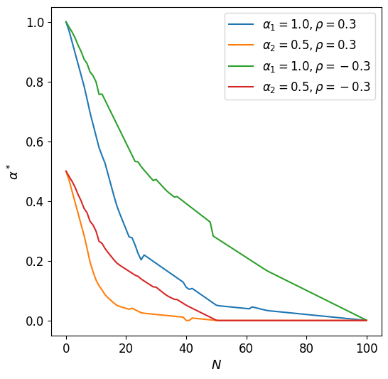
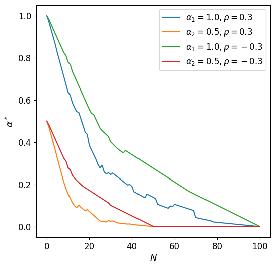


We extend the experiment to to study the affects of correlation with the proposed method. Since we directly consider the number of shares of an asset held instead of the proportion, we do not need to worry about adding additional constraints to the problem. In experiment , we only look at the selling agents and consider cases to study the affects of correlation in the order execution problem. In case , we simulate good market conditions , . In case , we simulate poor market conditions , . In case , we simulate mixed market conditions , . We study the affects of correlation between assets and . We set weak positive correlation as and strong positive correlation as . We set weak negative correlation as and strong negative correlation as .
Case :
In case , we set and . Figure 8 shows the optimal portfolio for each asset with high and low correlations. We also explore the case of positive and negative correlation. The top row shows the optimal portfolio for agent (left) and agent (right) with weak correlation. The bottom left and right figures show the optimal portfolio of the agents for strong correlation. Due to the non-uniqueness of the optimal trade rate, there is no uniqueness in the optimal portfolios.
We observe that when assets are negatively correlated, the agents tend to hold more risky assets than when they are positively correlated. Positively correlated assets sell more quickly because when one asset is sold, the price impact increases the value of correlated assets, prompting the agent to sell off assets faster. Asset is held longer to reduce the overall impact when the agent liquidates their position. Figure 9 shows the optimal control for each agent in assets with low correlation (top left and right) and high correlation (bottom left and right).


In Figure 9, we observe that the trade rates of each agent is more negative for positively correlated assets which implies that they are selling at a faster rate. In contrast, for negatively correlated assets, the trade rate is less negative resulting in slower liquidation of the risky assets. This results in a larger position in the risky asset held over time. Figure 9 shows the same trade rate for assets and at . This implies that the agents do not have a strong preference on holding asset or when they first begin to trade.
Case :
In case , we set and . Case assumes that both assets are under poor market conditions. Figure 10 plots the optimal portfolio for agents and when the assets are weakly and strongly correlated. The corresponding optimal controls are plotted in Figure 11.

In Figure 10, we observe that for weakly correlated assets, the agents actively liquidated assets regardless of correlation. However, under strong correlation negatively correlated, assets are liquidated more gradually. This is in line with what was observed in case . Since the two assets are negatively correlated, the agents expect asset to increase when asset decreases, and vice versa. This factor reduces the negative drift experienced by each asset, resulting in the agents liquidating the assets more gradually.


In Figure 11, the agents liquidate positively correlated more quickly at . This reflects the initial steeper slope shown for positively correlated assets. Note, the path of the controls is not unique in our problem, as the HJB equation only guarantees uniqueness of the value function.
Case :
In case , we set , and . Figure 12 plots the optimal portfolio of agent and agent when and . The optimal control of agent and agent are shown in Figure 13.


In Figure 12, we observe that when there are mixed market conditions, the agents try to liquidate the assets in a similar manner regardless of correlation. Both negative and positive correlation encourages the agents to gradually liquidate asset as asset is expected to increase its price over time. In Figure 13, we see the agents quickly liquidating asset . We also observe that the agents actually do not liquidate asset completely until the assets are sold off at .
5.4 Experiment 4: Optimal Execution for 2 Agents with Different Price Impact
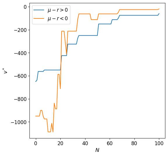
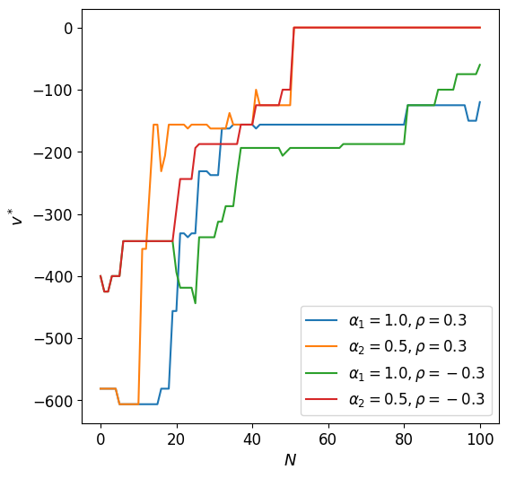
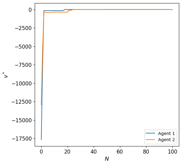
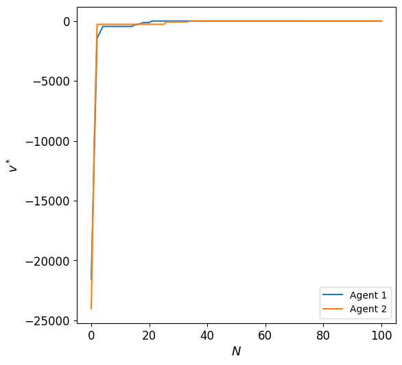
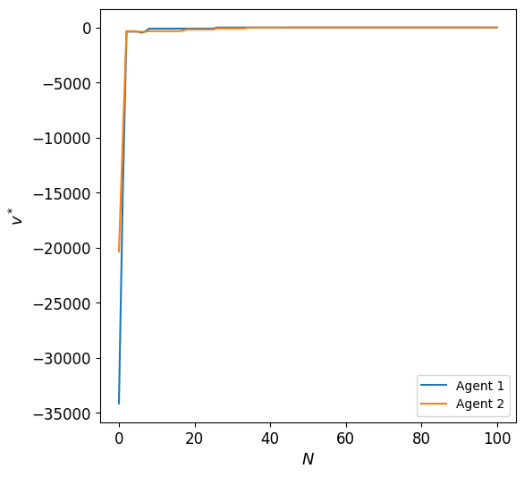
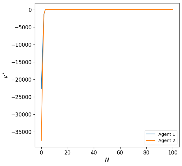
In this experiment, we study the interaction of two agents with different permanent price impact factors, . Agent has and agent has . This signifies that agent is a very influential trading agent who has a lot of impact on price dynamics. Conversely, agent is a trading agent with no price impact at all. We study the interaction between the agents for asset and observe how they interact in a good economy, i.e. and in a bad economy, i.e. . We also consider the different levels of performance awareness, . We set , or , , , , and for , , .


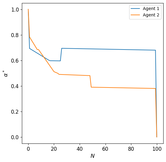
First, we consider the case when . The optimal portfolio and trade rate for agent and agent are shown in Figure 14. We observe that when , agent is very inactive in their trading activity and holds a large proportion of wealth in risky assets. Agent on the other hand sells off their position consistently until around .
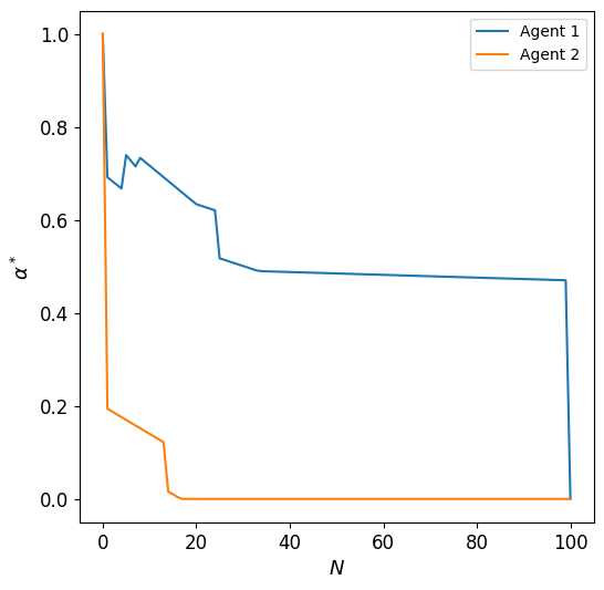
The trade rates tell us that agent perceives the market to be more risky than agent . This can be seen in the trade rates, where agent sells off more quickly than agent . When , we observe an interesting behaviour. Agent immediately sells off their position. There is no penalty for agent to do this as they have no impact on the asset price. However, agent does not do the same and actually holds a large position in the risky asset longer before liquidating fully.

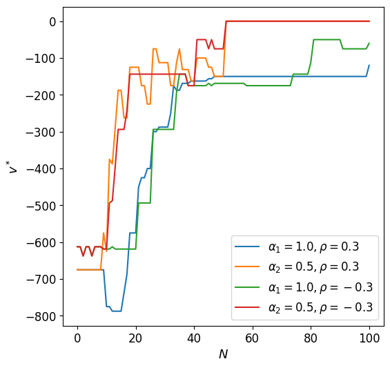
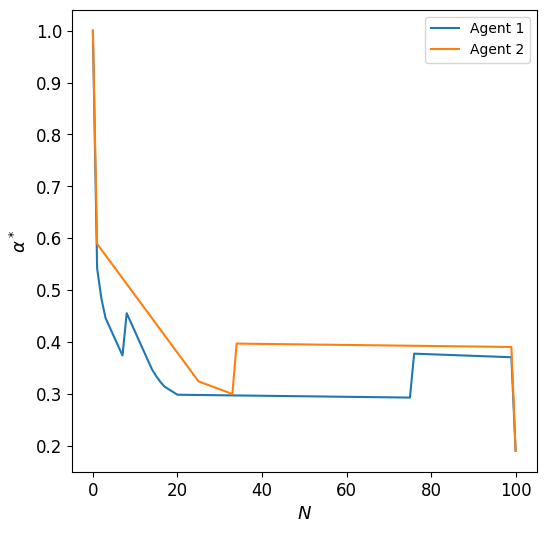
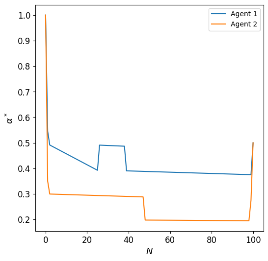
Next, we consider the case when . The optimal portfolio and trade rate for agent and agent are shown Figure 15. In this case, both agents are aware of the general performance of the other agent and they both sell quickly. When , both agents want to hold more positions in the risky asset until the moment they want to liquidate after , this is expected as the payoff from holding the asset until outweighs the penalty from failing to liquidate in the time horizon when . We see that agent trades faster than agent until around , but the trading eases as goes to . When , we see a similar behaviour to the good economy case for agent except that agent trades faster until around . We see agent trade more gradually until as it would see the asset price drop due to the actions of agent .
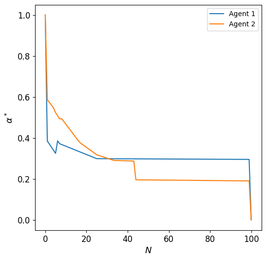
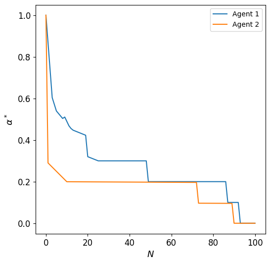
Finally, we consider the case when . In Figure 16, we observe that agent is willing to hold more position in the risky asset but not as quickly as when . This is because both agents now weigh the average performance of the market almost as much as their own individual performance. When , again both agents want to hold more positions in the risky asset until the moment they want to liquidate after . We see that agent trades faster than agent at all timesteps. When , agent sells more actively than agent which in turn lowers the asset price. In response, agent reduces their position in the risky asset drastically from the start.
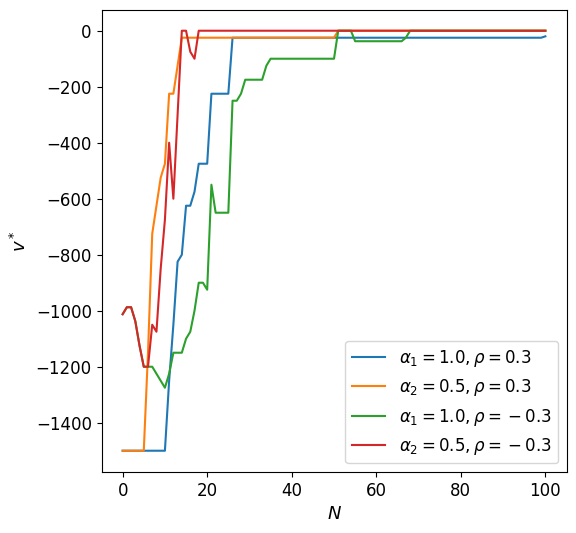
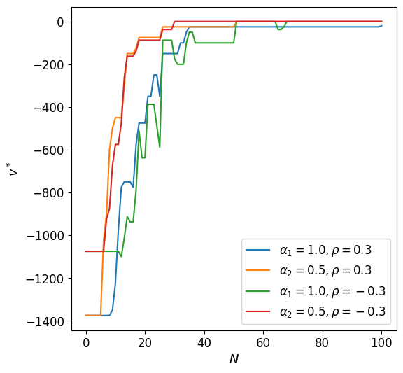
5.5 Experiment 5: Optimal Execution for Multiple Buyers and Sellers
In this experiment, we compare the investment performance between sellers (long) and buyers (short) in different economic conditions. To compare different groups of agents, we compute the average Sharpe ratio of the selling agents and the buying agents. The Sharpe ratio provides an insight into the relative performance of the portfolio return. A positive Sharpe ratio is considered an investment strategy that outperforms the risk free rate. A negative Sharpe ratio indicates the liquidating strategy; i.e. selling and buying, have lower return than holding the asset. In our problem, a strategy with Sharpe ratio is acceptable.
For each agent , the return on liquidating the position is given by and the standard deviation on the return is . We want to compare the strategy with the strategy of holding the asset from to . The no-trade return is given by . Thus the Sharpe ratio is given by:
Note we compare the portfolio with the expected value of the asset instead of the risk free rate of return. This compares the performance of different strategies versus holding the asset without liquidating. If the number of long agents is given by and the number of short agents is given by , then we can compute
to measure the average performance of the long agents (buyers) and short agents (sellers) respectively.
We simulate agents and assets with . We do not consider correlation in this example so that the results are easier to understand. In this experiment, we set for , , , and fix . By increasing the number of agents beyond , we can study more interesting dynamics between agents. In case , we let agents be selling agents and agents be buying agents. Selling agents are agents liquidating long positions and buying agents are agents liquidating short positions. In case , we look at the selling and buying agents. In case , we look at the case where we have selling agents and buying agents. For all three cases, we consider different market conditions:
-
1.
good market conditions ,
-
2.
poor market conditions ,
-
3.
mixed market conditions .
Case : selling agents, buying agents
In case , we look at the average Sharpe ratio of selling agents and buying agents in different market conditions. The average Sharpe ratio for sellers and buyers are summarized in Table 5. We observe that under market conditions and , it is advantageous for selling and buying agents to liquidate. The best Sharpe ratio we achieve is for selling agents under . This is because the agents liquidate the short positions gradually and the long positions quickly. There is an overall negative price impact due to the asymmetry in the number of sellers and buyers which leads to lower asset prices. Under market conditions , it is disadvantageous to liquidate short positions over holding the asset. This occurs from the overall negative price impact that decreases the amount of growth for both assets. Due to the imbalance of sellers and buyers, we observe the selling agent always performing better than the holding strategy.
| Market Condition | ||
|---|---|---|
Case : selling agents, buying agents
In case , we look at the average Sharpe ratio of selling agents and buying agents in different market conditions. The average Sharpe ratio for sellers and buyers are summarized in Table 6.
| Market Condition | ||
|---|---|---|
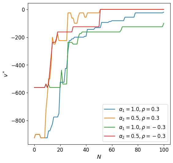
We observe that under market conditions and , it is advantageous for long and short agents to liquidate. The best Sharpe ratio we achieve is for sellers under . This is because agents sell (buy) asset more gradually (quickly) and asset more quickly (gradually). Because , the agents gain more from the increase in asset price than the decrease in asset price. This results in an advantage for gradual sellers and aggressive buyers. Under , sellers have an advantage since they sell off gradually and the price of both assets are expected to increase. Buyers are disadvantaged as the expected value of the asset increases under , even if they liquidate quickly.
Case : selling agents, buying agents
In case , we look at the average Sharpe ratio of selling agents and buying agents in market conditions , and . The average Sharpe ratio for sellers and buyers are summarized in Table 7. We observe that under market conditions , it is advantageous for sellers and buyers to liquidate. The best Sharpe ratio we achieve is for selling agents under . There is an overall positive price impact since the number of buyers is greater than the number of sellers. We see that sellers and buyers generally do not out perform the hold strategy. This is due to the overall positive price impact adding to the drift term of both assets pushing up the asset price.
| Market Condition | ||
|---|---|---|
6 Conclusion
In this paper, we extended the optimal trade execution problem under the Markowitz criteria to a time-consistent optimal trade execution problem for multiple assets and multiple agents setting. This is done by formulating the original mean-variance problem into its dual representation coupled with an auxiliary HJB equation Aivaliotis and Veretennikov [2018]. To extend this into higher dimensions, we reformulate the auxiliary HJB equation into a BSDE that can be solved using a neural network. We present a deep residual self-attention network to solve the BSDE presented in (21). This allows us to use a deep residual network that learns temporal dependencies. This overcomes the issue of saving weights for every timestep and overcomes the vanishing gradient problem of recurrent networks Na and Wan [2023].
We show in Experiment that the proposed method matches classical solutions where applicable. In Experiment we show sensitivities of the proposed method with respect to . When an agent is more conscious other agents in the market, i.e. increases, agents tend to invest more in risky assets. When an agent is more risk adverse, i.e. increases, the agent invests less in risky assets. We saw that as the temporary price impact of the agent increases they tend to liquidate more gradually and as the permanent price impact increases the agents liquidate faster.
In Experiment , we looked at the optimal execution of agents under different market conditions. With we saw that the agents liquidated assets gradually when the market conditions were good and liquidated quickly when they were poor. We also looked at the affects of strong and weak correlation with . In Experiment , we study the interaction between agents, where one agent contributed all the price impact. We found that in general as increase we see decreased trading activity from agent , we also see agent hold less risky assets. In good economic conditions agent holds larger positions in the risky asset and is less active in trading than in poor economic conditions.
In Experiment , we studied the average performance of a group of sellers and buyers in different economic conditions in a market consisting of agents. We found that in most economic conditions active trading on both sides of the market benefited sellers and buyers. In any scenario, when the economy was good, buyers underperformed the hold position. In the case of sellers and buyers both sellers and buyers underperformed the holding strategy, except when both assets are expected to reduce in price.
Disclosure Statement
No potential conflict of interest is reported by the author(s).
Funding
This work was supported by the Natural Sciences and Engineering Research Council of Canada.
ORCID
-
Andrew Na: https://orcid.org/ 0000-0002-6162-8171
-
Justin W.L. Wan: https://orcid.org/ 0000-0001-8367-6337
References
- Aivaliotis and Palczewski [2014] Georgios Aivaliotis and Jan Palczewski. Investment strategies and compensation of a mean–variance optimizing fund manager. European Journal of Operational Research, 234(2):561–570, 2014. ISSN 0377-2217. doi:https://doi.org/10.1016/j.ejor.2013.04.038. URL https://www.sciencedirect.com/science/article/pii/S0377221713003524. 60 years following Harry Markowitz’s contribution to portfolio theory and operations research.
- Aivaliotis and Veretennikov [2018] Georgios Aivaliotis and A.Yu. Veretennikov. An HJB approach to a general continuous-time mean-variance stochastic control problem. Random Operators and Stochastic Equations, 26(4):225–234, 2018. doi:doi:10.1515/rose-2018-0020. URL https://doi.org/10.1515/rose-2018-0020.
- Alfonsi et al. [2010] Aurélien Alfonsi, Antje Fruth, and Alexander Schied. Optimal execution strategies in limit order books with general shape functions. Quantitative Finance, 10(2):143–157, 2010. doi:10.1080/14697680802595700. URL https://doi.org/10.1080/14697680802595700.
- Almgren and Chriss [2000] Robert Almgren and Neil A. Chriss. Optimal execution of portfolio transactions. 2000.
- Basak and Chabakauri [2010] Suleyman Basak and Georgy Chabakauri. Dynamic mean-variance asset allocation. The Review of Financial Studies, 23(8):2970–3016, 2010. ISSN 08939454, 14657368. URL http://www.jstor.org/stable/40782974.
- Bergault et al. [2022] Philippe Bergault, Fayçal Drissi, and Olivier Guéant. Multi-asset optimal execution and statistical arbitrage strategies under Ornstein-Uhlenbeck dynamics. SIAM Journal on Financial Mathematics, 13(1):353–390, 2022. doi:10.1137/21M1407756. URL https://doi.org/10.1137/21M1407756.
- Bjork et al. [2017] Thomas Bjork, Mariana Khapko, and Agatha Murgoci. On time-inconsistent stochastic control in continuous time. Finance and Stochastics, 21(2):331–360, 2017. doi:10.1007/s00780-017-0327-5.
- Cartea and Jaimungal [2016] Alvaro Cartea and Sebastian Jaimungal. Incorporating order-flow into optimal execution. volume 10, pages 339–364, 2016. doi:10.1007/s11579-016-0162-z.
- Chen et al. [2022] Di Chen, Yada Zhu, Miao Liu, and Jianbo Li. Cost-efficient reinforcement learning for optimal trade execution on dynamic market environment. In Proceedings of the Third ACM International Conference on AI in Finance, ICAIF ’22, page 386–393, New York, NY, USA, 2022. Association for Computing Machinery. ISBN 9781450393768. doi:10.1145/3533271.3561761. URL https://doi.org/10.1145/3533271.3561761.
- Chen and Wan [2021] Yangang Chen and Justin W. L. Wan. Deep neural network framework based on backward stochastic differential equations for pricing and hedging American options in high dimensions. Quantitative Finance, 21(1):45–67, 2021. doi:10.1080/14697688.2020.1788219. URL https://doi.org/10.1080/14697688.2020.1788219.
- E et al. [2017] Weinan E, Jiequn Han, and Arnulf Jentzen. Deep learning-based numerical methods for high-dimensional parabolic partial differential equations and backward stochastic differential equations. Communications in Mathematics and Statistics, 5:349–380, Nov 2017.
- Forsyth [2011] Peter A. Forsyth. A Hamilton–Jacobi–Bellman approach to optimal trade execution. Applied Numerical Mathematics, 61(2):241–265, 2011. ISSN 0168-9274. doi:https://doi.org/10.1016/j.apnum.2010.10.004. URL https://www.sciencedirect.com/science/article/pii/S0168927410001789.
- Forsyth [2020] Peter A. Forsyth. Multiperiod mean conditional value at risk asset allocation: Is it advantageous to be time consistent? SIAM J. Fin. Math., 11(2):358–384, jan 2020. doi:10.1137/19M124650X. URL https://doi.org/10.1137/19M124650X.
- Goodfellow et al. [2016] I. Goodfellow, Y. Bengio, and A. Courville. Deep learning, adaptive computation and machine learning. MIT Press, Cambridge, MA, 2016.
- Guan and Hu [2022] Guohui Guan and Xiang Hu. Time-consistent investment and reinsurance strategies for mean–variance insurers in N-agent and mean-field games. North American Actuarial Journal, 26(4):537–569, 2022. doi:10.1080/10920277.2021.2014891. URL https://doi.org/10.1080/10920277.2021.2014891.
- Han and E [2016] Jiequn Han and Weinan E. Deep learning approximation for stochastic control problems, 2016.
- He et al. [2016] Kaiming He, Xiangyu Zhang, Shaoqing Ren, and Jian Sun. Deep residual learning for image recognition. In 2016 IEEE Conference on Computer Vision and Pattern Recognition (CVPR), pages 770–778, 2016. doi:10.1109/CVPR.2016.90.
- Hendricks and Wilcox [2014] Dieter Hendricks and Diane Wilcox. A reinforcement learning extension to the Almgren-Chriss framework for optimal trade execution. In 2014 IEEE Conference on Computational Intelligence for Financial Engineering & Economics (CIFEr), pages 457–464, 2014. doi:10.1109/CIFEr.2014.6924109.
- Hure et al. [2020] Come Hure, Huyen Pham, and Xavier Warin. Deep backward schemes for high-dimensional nonlinear PDEs. Mathematics of Computation, 2020.
- Kingma and Ba [2017] D.P. Kingma and J. Ba. Adam: A method for stochastic optimization, 2017.
- Li and Ng [2000] Duan Li and Wan-Lung Ng. Optimal dynamic portfolio selection: Multiperiod mean-variance formulation. Mathematical Finance, 10(3):387–406, 2000. doi:https://doi.org/10.1111/1467-9965.00100. URL https://onlinelibrary.wiley.com/doi/abs/10.1111/1467-9965.00100.
- Lin and Beling [2021] Siyu Lin and Peter A. Beling. A deep reinforcement learning framework for optimal trade execution. In Yuxiao Dong, Georgiana Ifrim, Dunja Mladenić, Craig Saunders, and Sofie Van Hoecke, editors, Machine Learning and Knowledge Discovery in Databases. Applied Data Science and Demo Track, pages 223–240, Cham, 2021. Springer International Publishing. ISBN 978-3-030-67670-4.
- Na and Wan [2023] Andrew S. Na and Justin W. L. Wan. Efficient pricing and hedging of high-dimensional American options using deep recurrent networks. Quantitative Finance, 23(4):631–651, 2023. doi:10.1080/14697688.2023.2167666. URL https://doi.org/10.1080/14697688.2023.2167666.
- Ning et al. [2021] Brian Ning, Franco Ho Ting Lin, and Sebastian Jaimungal. Double deep q-learning for optimal execution. Applied Mathematical Finance, 28(4):361–380, 2021. doi:10.1080/1350486X.2022.2077783. URL https://doi.org/10.1080/1350486X.2022.2077783.
- Pham [2014] Huyen Pham. Feynman-Kac representation of fully nonlinear pdes and applications. Acta Mathematica Vietnamica, 40:255–269, 2014. URL https://api.semanticscholar.org/CorpusID:19184753.
- Ronneberger et al. [2015] Olaf Ronneberger, Philipp Fischer, and Thomas Brox. U-net: Convolutional networks for biomedical image segmentation, 2015. URL http://arxiv.org/abs/1505.04597. cite arxiv:1505.04597Comment: conditionally accepted at MICCAI 2015.
- Schoneborn [2008] Torsten Schoneborn. Trade execution in illiquid markets Optimal stochastic control and multi-agent equilibria. PhD thesis, Technical University of Berlin, 2008.
- Tse [2012] Shu-tong Tse. Numerical Methods for Optimal Trade Execution. PhD thesis, David R. Cheriton School of Computer Science, University of Waterloo, 2012.
- Van Staden et al. [2018] Pieter M. Van Staden, Duy-Minh Dang, and Peter A. Forsyth. Time-consistent mean–variance portfolio optimization: A numerical impulse control approach. Insurance: Mathematics and Economics, 83:9–28, 2018. ISSN 0167-6687. doi:https://doi.org/10.1016/j.insmatheco.2018.08.003. URL https://www.sciencedirect.com/science/article/pii/S0167668718301252.
- Vaswani et al. [2017] Ashish Vaswani, Noam Shazeer, Niki Parmar, Jakob Uszkoreit, Llion Jones, Aidan N Gomez, Ł ukasz Kaiser, and Illia Polosukhin. Attention is all you need. In I. Guyon, U. Von Luxburg, S. Bengio, H. Wallach, R. Fergus, S. Vishwanathan, and R. Garnett, editors, Advances in Neural Information Processing Systems, volume 30. Curran Associates, Inc., 2017. URL https://proceedings.neurips.cc/paper_files/paper/2017/file/3f5ee243547dee91fbd053c1c4a845aa-Paper.pdf.
- Vigna [2020] Elena Vigna. On time consistency for mean-variance portfolio selection. International Journal of Theoretical and Applied Finance, 23(06):2050042, 2020. doi:10.1142/S0219024920500429. URL https://doi.org/10.1142/S0219024920500429.
- Wang and Zhou [2020] Haoran Wang and Xun Yu Zhou. Continuous-time mean–variance portfolio selection: A reinforcement learning framework. Mathematical Finance, 30(4):1273–1308, 2020. doi:https://doi.org/10.1111/mafi.12281. URL https://onlinelibrary.wiley.com/doi/abs/10.1111/mafi.12281.
- Wang and Forsyth [2011] J. Wang and P.A. Forsyth. Continuous time mean variance asset allocation: A time-consistent strategy. European Journal of Operational Research, 209(2):184–201, 2011. ISSN 0377-2217. doi:https://doi.org/10.1016/j.ejor.2010.09.038. URL https://www.sciencedirect.com/science/article/pii/S0377221710006363.
- Zhou and Li [2000] X.Y. Zhou and D. Li. Continuous-time mean-variance portfolio selection: A stochastic LQ framework. Applied Mathematics and Optimization, 42(1):19–33, 2000. doi:10.1007/s002450010003.