Quantifying the Uncertainty of Sensitivity Coefficients Computed from Uncertain Compound Admittance Matrix and Noisy Grid Measurements

Abstract

The power-flow sensitivity coefficients (PFSCs) are widely used in the power system for expressing linearized dependencies between the controlled (i.e., the nodal voltages, lines currents) and control variables (e.g., active and reactive power injections, transformer tap positions, etc.). The PFSCs are often computed by knowing the compound admittance matrix of a given network and the grid states. However, when the branch parameters (or admittance matrix) are inaccurate or known with limited accuracy, the computed PFSCs can not be relied upon. Uncertain PFSCs, when used in control, can lead to infeasible control set-points. In this context, this paper presents a method to quantify the uncertainty of the PFSCs from uncertain branch parameters and noisy grid-state measurements that can be used for formulating safe control schemes. We derive an analytical expression using the error-propagation principle. The developed tool is numerically validated using Monte Carlo simulations.

I Introduction

The non-linearities of the optimal power flow (OPF) are often tackled by its linearization, e.g., in [1] where the derivatives of the controlled variables with respect to the control variables (referred to as power-flow sensitivity coefficients – PFSCs) are used for expressing linear models of the grid constraints. The PFSCs are used in key applications such as voltage control [2], congestion management [3], loss minimization, dispatching [4], etc. However, the computed PFSC might be uncertain due to inaccuracy in the grid parameters or noisy grid measurements. Therefore, to obtain a reliable control of active distribution networks (ADNs), there is a need to quantify the uncertainty on the PFSCs such that those can be considered in the uncertainty-aware control formulation.

In the existing literature, PFSC computation techniques can be broadly categorized into two types. The first is referred to as model-based schemes, i.e., when the admittance parameters of the network are accurately known, for example, in [5, 6, 7]. The second referred to measurement-based control schemes, use measurements to estimate the PFSCs, for example in [8, 9, 10] etc. Both schemes may suffer from inaccuracies. When fed with uncertain admittance parameters, the model-based schemes lead to inaccurate and uncertain PFSCs. Similarly, the measurement-based schemes are prone to noises of the measuring units resulting in inaccurate estimates. Most existing works have focused on developing better estimation techniques for the PFSCs. Still, to the best of the author’s knowledge, none of the schemes have quantified the amount of uncertainties on the computed/estimated PFSCs. Currently, the PFSC uncertainty is characterized by computationally expensive Monte-Carlo simulations [2] and then accounted for in the control problem. In [10], the uncertainty is derived from a measurement-based tool-chain using nodal voltage and power measurements.

In this context, this work proposes a method to quantify uncertainty in PFSC computation. We refer to the case when PFSC is computed using the compound admittance matrix as in [6]. In particular, we derive an analytical uncertainty propagation tool using the principle of error propagation that is a function of admittance parameters, grid measurements and their respective uncertainties quantified by their variances and covariances. To the best of the author’s knowledge, this is the first work quantifying uncertainty analytically from uncertain branch parameters in sensitivity coefficients. Compared to [2], the proposed scheme is faster and straightforward.

The paper is organized as follows. Section II presents problem statement, Section III recalls a method to compute PFSCs using compound admittance matrix, Section IV presents the proposed uncertainty propagation method for PFSCs from uncertain compound admittance matrix, Section V presents the numerical validation of the proposed scheme, and finally, Section VI summarizes the main findings of this work.

II Problem Statement

We consider a generic power network for which we want to compute the PFSCs. For the sake of brevity, we limit the description to the computation of the voltage sensitivity coefficients and their uncertainties; other sensitivity coefficients can be similarly computed. The objective is to assess the uncertainty of computed voltage sensitivity coefficients and their mean value by propagating the admittance parameter inaccuracies and grid measurements noise. The proposed tool is then numerically validated by the Monte Carlo approach for an IEEE benchmark network.

III Compound Admittance Matrix-based Sensitivity Coefficient Computation

In the following, we recall a method for computing the PFSCs using the compound admittance matrix, originally developed in [6] and extended in [12]. The PFSC computation scheme relies on information on the compound admittance matrix and grid states. The method computes the PFSCs by solving a set of linear equations and guarantees a unique solution, given that the Jacobian of the load flow solution is invertible [13].

We assume a three-phase network configuration where the phases are denoted by $a,b$, and $c$, and let the number of phases be denoted by $p$, i.e., $p=3$ in this case. Let the symbols $N_{b}$ and $\mathcal{N}_{b}=\{1,\dots,N_{b}\}$ refer to the number of buses/nodes and the set containing indices of the nodes in a generic network. Let the phase-to-ground nodal voltages be denoted by $\bar{\boldsymbol{E}}=[\bar{E}^{a}_{1},\bar{E}^{b}_{1},\bar{E}^{c}_{1},\cdots,\bar{E}^{a}_{{N}_{b}},\bar{E}^{b}_{{N}_{b}},\bar{E}^{c}_{{N}_{b}}]$. Let the nodal apparent power injections are denoted by $\bar{\boldsymbol{S}}=[\bar{S}^{a}_{1},\bar{S}^{b}_{1},\bar{S}^{c}_{1},\cdots,\bar{S}^{a}_{{N}_{b}},\bar{S}^{b}_{{N}_{b}},\bar{S}^{c}_{{N}_{b}}]$, with $\bar{S}^{\phi}_{i}=P^{\phi}_{i}+jQ^{\phi}_{i}$ where $P^{\phi}_{i}$ and $Q^{\phi}_{i}$ are active and reactive powers, respectively, for phase $\phi\in\{a,b,c\}$, node $i\in\mathcal{N}_{b}$; $\bar{S}^{\phi}_{i}$ is expressed as

$$\bar{S}^{\phi}_{i}=\bar{E}^{\phi}_{i}\sum_{\begin{subarray}{c}n\in\mathcal{N}_{b}\\ \phi^{\prime}\in\{a,b,c\}\end{subarray}}\underline{Y}_{in}^{\phi\phi^{\prime}}\underline{E}_{n}^{\phi^{\prime}} {\color[rgb]{0,0,0}\forall i\in\mathcal{N}_{b},\phi\in\{a,b,c\}}$$ (1)

where, $\bar{Y}^{\phi,\phi^{\prime}}_{in}$ ($\phi,\phi^{\prime}\in\{a,b,c\}$) refers to an element of the admittance matrix referring to the line connecting between $i-$th and $n-$th nodes for in the compound admittance matrix $\bar{\mathbf{Y}}$ and mutual admittance between phases $\phi$ and $\phi^{\prime}$.

Following the approach in [6, 12], we differentiate the equation in (1) with respect to active power and reactive power injections $P^{\phi^{\prime}}_{l},Q^{\phi^{\prime}}_{l},l\in\mathcal{N}_{b},\psi\in\{a,b,c\}$, it results in

$$\mathbb{1}_{\begin{subarray}{c}i=l,\\ \psi=\phi\end{subarray}}=\frac{{}\partial{\underline{E}^{\phi}_{i}}}{\partial{P_{l}^{\psi}}}\sum_{\begin{subarray}{c}n\in\mathcal{N}_{b}\\ \phi^{\prime}\in\{a,b,c\}\end{subarray}}{\bar{Y}}^{\phi\phi^{\prime}}_{in}\bar{E}^{\phi^{\prime}}_{n}+\underline{E}^{\phi}_{i}\sum_{\begin{subarray}{c}n\in\mathcal{N}_{b}\\ \phi^{\prime}\in\{a,b,c\}\end{subarray}}{\bar{Y}}^{\phi\phi^{\prime}}_{in}\frac{{}\partial{\bar{E}^{\phi^{\prime}}_{n}}}{\partial{P}^{\psi}_{l}},$$ (2)

$$-j\mathbb{1}_{\begin{subarray}{c}i=l,\\ \psi=\phi\end{subarray}}=\frac{{}\partial{\underline{E}^{\phi}_{i}}}{\partial{Q}^{\psi}_{l}}\sum_{\begin{subarray}{c}n\in\mathcal{N}_{b}\\ \phi^{\prime}\in\{a,b,c\}\end{subarray}}{\bar{Y}}^{\phi\phi^{\prime}}_{in}\bar{E}^{\phi^{\prime}}_{n}+\underline{E}^{\phi}_{i}\sum_{\begin{subarray}{c}n\in\mathcal{N}_{b}\\ \phi^{\prime}\in\{a,b,c\}\end{subarray}}{\bar{Y}}^{\phi\phi^{\prime}}_{in}\frac{{}\partial{\bar{E}^{\phi^{\prime}}_{n}}}{\partial{Q}^{\psi}_{l}}$$ (3)

where $\frac{\partial{\square}}{\partial{\square}}$ refers to the partial derivatives. Here, $\mathbb{1}_{\begin{subarray}{c}i=l,\\ \psi=\phi\end{subarray}}$ denotes a vector of zeros with 1 when ${\{i=l\}}$ and ${\{\psi=\phi\}}$ are satisfied. Rearranging the rows/columns of the eq. (2)-(3) for different nodes, the set of linear equations can be written as

$$\mathbf{z}=\mathbf{H}\mathbf{x}$$ (4)

where $\mathbf{H}\in\mathbb{R}^{2p(N_{b}-1)\times 2p(N_{b}-1)}$ and $\mathbf{z}\in\mathbb{R}^{{2p(N_{b}-1)}\times p(N_{b}-1)}$. The elements of the matrix $\mathbf{H}$ and vector $\mathbf{z}$ are obtained using [12]. Here, $\mathbf{x}\in\mathbb{R}^{{2p(N_{b}-1)}\times p(N_{b}-1)}$ is the vector of unknown sensitivities, i.e., $\frac{{}\partial{\bar{E}^{\phi}_{i}}}{\partial{P}^{\phi^{\prime}}_{l}}$ and $\frac{{}\partial{\underline{E}^{\phi}_{i}}}{\partial{P}^{\phi^{\prime}}_{l}}$, where $i,l\in\mathcal{N}_{b}$ and $\phi,\phi^{\prime}\in\{a,b,c\}$. The $\mathbf{x}$ can be obtained by

$$\mathbf{x}=\mathbf{H}^{-1}\mathbf{z}.$$ (5)

It should be remarked that the expression in (5) depends on the elements of the admittance matrix and the nodal voltage phasors. As both the admittance matrix and nodal voltages are assumed to be uncertain, we need to propagate the error into the computation of the sensitivity coefficients. This is described next.

IV Uncertainty Propagation: From Uncertain Compound Admittance Matrix to the PFSCs

As anticipated, the elements of the $\mathbf{H}$ in eq. (5) might be uncertain due to the inaccuracy of the compound admittance matrix ($\bar{\mathbf{Y}}$) and the noise introduced by the measuring instruments. Therefore, the error on the $\bar{\mathbf{Y}}$ and grid voltage measurement $\bar{\boldsymbol{E}}$ needs to be propagated to evaluate the uncertainty on $\mathbf{x}$ in (5). The objective would be to compute the variance of the uncertainty coefficients contained in vector $\mathbf{x}$.

Hypothesis 1:

It is assumed that the measurement uncertainty on real and imaginary parts of $\bar{\boldsymbol{E}}$ can be modeled by Gaussian distribution, i.e., $\Re\{{\tilde{\bar{\boldsymbol{E}}}}\}\in\mathscr{N}(\Re\{{{\bar{\boldsymbol{E}}}}\},\boldsymbol{\sigma}^{\Re}_{{{\bar{\boldsymbol{E}}}}})$ and $\Im\{{\tilde{\bar{\boldsymbol{E}}}}\}\in\mathscr{N}(\Im\{{{\bar{\boldsymbol{E}}}}\},\boldsymbol{\sigma}^{\Im}_{{{\bar{\boldsymbol{E}}}}})$ with $\Re$ and $\Im$ denotes the real and imaginary parts of a complex number, $\tilde{\bar{\boldsymbol{E}}}$ the measurements of $\bar{\boldsymbol{E}}$ with noise, $\boldsymbol{\sigma}^{\Re}_{{{\bar{\boldsymbol{E}}}}}$ and $\boldsymbol{\sigma}^{\Im}_{{{\bar{\boldsymbol{E}}}}}$ the standard (std.) deviations on measurement uncertainty for $\Re\{{{\bar{\boldsymbol{E}}}}\}$ and $\Im\{{{\bar{\boldsymbol{E}}}}\}$, respectively. Appendix -1 shows the expressions to compute real and imaginary variances for voltage phasors under a realistic noise model (from magnitudes and phase). Appendix -2 validates the Gaussian assumption by quantile-quantile (QQ) plots.

Hypothesis 2:

It is assumed that the uncertainty on the real and imaginary parts of the elements of the compound admittance matrix can be modeled by Gaussian distributions.

Remark: In (5), the elements of $\mathbf{H}$ have multiplicative and additive elements consisting of elements of $\bar{\mathbf{Y}}$ and $\bar{\boldsymbol{E}}$ whose variances are known individually. So, to compute the variance of elements of $\mathbf{H}$, we use propagation of uncertainty for multiplicative and additive error propagation rules. They are

$$\sigma(\Theta+\Phi)^{2}\approx\sigma_{\Theta}^{2}+\sigma_{\Phi}^{2}+2\sigma_{\Theta\Phi,}$$ (6a)

$$\sigma(\Theta\times\Phi)\approx\Theta^{2}\Phi^{2}(\sigma_{\Theta}^{2}/{\Theta}^{2}+\sigma_{\Phi}^{2}/{\Phi}^{2}+2\sigma_{\Theta\Phi}/{\Theta\Phi}).$$ (6b)

Let $[\sigma_{\mathbf{H}^{-1}}]$ be the std. deviation of matrix $\mathbf{H}^{-1}$, $[\sigma_{\mathbf{H}^{-1}}]_{ij}$ be the std. deviation of $ij-$th element of $\mathbf{H}^{-1}$, $[\sigma_{\mathbf{x}}]_{i}$ be the std. deviation of $i-$th element of $\mathbf{x}$, and $[\sigma_{\mathbf{z}}]_{j}$ be the variance of $j-$th element of $\mathbf{z}$. Using the principle of error propagation, variance on $\mathbf{x}$ can be approximated as

$$[\sigma_{\mathbf{x}}]_{i}^{2}=\sum_{j}\Big{(}[\mathbf{H}^{-1}]^{2}_{ij}[\sigma_{\mathbf{z}}]_{j}^{2}+{[\sigma_{\mathbf{H}^{-1}}]_{ij}^{2}}[\mathbf{z}]_{j}^{2}\Big{)}.$$ (7a)

As $\mathbf{z}$ in (4) is constant (consisting of 0’s or 1’s), $\sigma_{\mathbf{z}}=0$, the expression in (7a) reduces to

$$[\sigma_{\mathbf{x}}]_{i}^{2}=\sum_{j}{[\sigma_{\mathbf{H}^{-1}}]_{ij}^{2}}[\mathbf{z}]_{j}^{2}.$$ (7b)

In (7b), $[\sigma_{\mathbf{H}^{-1}}]$ is unknown, it can be computed by propagating the variance of the elements of $\mathbf{H}$ by following relation (as described in [14]), the self-correlation is given by

$$[\sigma_{\mathbf{H}^{-1}}]_{mn}^{2}=\sum_{i}\sum_{j}[\mathbf{H}^{-1}]_{{mi}}^{2}[\sigma_{\mathbf{H}}]_{ij}^{2}[\mathbf{H}^{-1}]_{jn}^{2}$$ (7c)

and cross-correlation is given by

$$\begin{aligned} &{\text{cov}(\mathbf{H}^{-1}_{mn},\mathbf{H}^{-1}_{ab})}=~{}~{}~{}~{}~{}~{}~{}\\ &\sum_{i}\sum_{j}[\mathbf{H}^{-1}]_{mi}[\mathbf{H}^{-1}]_{ai}[\sigma_{\mathbf{H}}]_{ij}^{2}[\mathbf{H}^{-1}]_{jn}[\mathbf{H}^{-1}]_{jb}\end{aligned}$$ (7d)

Since, the matrix inversion is a non-linear operation, and the elements of the inverse matrix ($\mathbf{H}^{-1}$) are statistically correlated. Therefore, variance of each element of the matrix $\mathbf{H}^{-1}$ is of size $2p(N_{b}-1)\times 2p(N_{b}-1)$ itself by considering correlation of each element with every element in the matrix. Therefore, the size of $\sigma_{\mathbf{H}^{-1}}$ is $4p^{2}(N_{b}-1)^{2}\times 4p^{2}(N_{b}-1)^{2}$.

TABLE I: Performance comparison with the number of samples in Monte-Carlo simulations.

		$\Re(\frac{\partial\bar{E}_{3}}{\partial P_{2}})$	$\Re(\frac{\partial\bar{E}_{3}}{\partial P_{4}})$	$\Re(\frac{\partial\bar{E}_{4}}{\partial P_{4}})$	$\Im(\frac{\partial\bar{E}_{3}}{\partial P_{2}})$	$\Im(\frac{\partial\bar{E}_{3}}{\partial P_{3}})$	$\Im(\frac{\partial\bar{E}_{4}}{\partial P_{4}})$	Computation time (sec)
Nominal value (p.u)		0.0071	0.0152	0.0239	0.0077	0.0176	0.0288	—-
Std. deviation (Analytical)		0.0006	0.0012	0.0018	0.0006	0.0011	0.0016	0.15
	$N_{\text{mc}}=$ 10	0.0009	0.0016	0.0021	0.0006	0.0012	0.0018	2.7
	$N_{\text{mc}}=$100	0.0007	0.0013	0.0020	0.0007	0.0013	0.0019	29.1
Std. deviation (Monte-Carlo)	$N_{\text{mc}}=$1000	0.0007	0.0014	0.0020	0.0007	0.0013	0.0019	282.7
	$N_{\text{mc}}=$10000	0.0007	0.0014	0.0020	0.0007	0.0013	0.0019	2785

TABLE II: Performance comparison with respect to uncertainty on the admittance matrix with $N_{\text{mc}}$ = 1000 and IT 1.0.

		$\Re(\frac{\partial\bar{E}_{3}}{\partial P_{2}})$	$\Re(\frac{\partial\bar{E}_{3}}{\partial P_{4}})$	$\Re(\frac{\partial\bar{E}_{4}}{\partial P_{4}})$	$\Im(\frac{\partial\bar{E}_{3}}{\partial P_{2}})$	$\Im(\frac{\partial\bar{E}_{3}}{\partial P_{3}})$	$\Im(\frac{\partial\bar{E}_{4}}{\partial P_{4}})$
$\sigma_{\bar{\mathbf{Y}}}$ (% of $\bar{\mathbf{Y}}$)	Nominal value, $x$ (p.u)	0.0071	0.0152	0.0239	0.0077	0.0176	0.0288
0.5	$\sigma_{x,\text{MC}}$ (% of $x$)	0.337e-3 (4.7%)	0.666e-3 (4.4%)	0.986e-3 (4.1%)	0.338e-3 (4.4%)	0.659e-3 (3.7%)	0.938e-3 (3.3%)
	$\sigma_{x,\text{AL}}$ (% of $x$)	0.334e-3 (4.7%)	0.662e-3 (4.4%)	0.991e-3 (4.1%)	0.316e-3 (4.1%)	0.628e-3 (3.6%)	0.900e-3 (3.1%)
1	$\sigma_{x,\text{MC}}$ (% of $x$)	0.0007 (9.9%)	0.0014 (9.2%)	0.0020 (8.4%)	0.0007 (9.1%)	0.0013 (7.4%)	0.0019 (6.6%)
	$\sigma_{x,\text{AL}}$ (% of $x$)	0.0006 (8.5%)	0.0012 (7.9%)	0.0018 (7.5%)	0.0006 (7.8%)	0.0011 (6.3%)	0.0016 (5.6%)
2	$\sigma_{x,\text{MC}}$ (% of $x$)	0.0015 (21.1%)	0.0030 (19.7%)	0.0044 (18.4%)	0.0014 (18.2%)	0.0028 (15.9%)	0.0040 (13.9%)
	$\sigma_{x,\text{AL}}$ (% of $x$)	0.0013 (18.3%)	0.0026 (17.1%)	0.0033 (13.8%)	0.0010 (13%)	0.0021 (11.9%)	0.0030 (10.4%)

V Numerical Validation

We numerically validate the proposed uncertainty estimation scheme using Monte Carlo simulations. The validation is performed on an IEEE benchmark network.

V-1 Simulation setup

The proposed estimation scheme is validated on an IEEE-4 benchmark network [15] (transposed line configuration) as shown in Fig. 1. The network is 24.9/4.16 kV, 10 MVA 3-phase operating in the balanced configuration. The grid hosts 300 kW/150 kVar of active/reactive power demand at nodes 2, 3 and and 4 and photovoltaic generation of 480 kWp and 600 kWp at nodes 2 and 3.

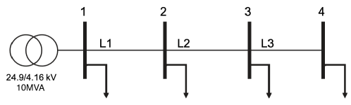
Figure 1: IEEE-4 balanced system.

For this performance evaluation, we use simulated synchrophasor noisy measurements from phasor measurement units (PMUs) on a network for which admittance parameters are known accurately. The noisy measurements are simulated as follows. First, load-flows are solved to compute the ground truth of the voltages phasors. Then, these phasors are added with noise in polar coordinates (i.e., in the magnitudes and phase). For the noise, we assume independent and identically distributed (i.i.d) and Gaussian distribution. The measurement noises are introduced in polar coordinates to reflect the real noise characteristics of instrument transformers (ITs). The ITs are characterized by magnitude and phase errors, specified in percentage for magnitudes and radians for phase angle. These values are characterized in [17] for different IT classes. The measurement noise is then projected on the rectangular coordinates to obtain $\boldsymbol{\sigma}^{\Re}_{{{\bar{\boldsymbol{E}}}}},\boldsymbol{\sigma}^{\Im}_{{{\bar{\boldsymbol{E}}}}}$ as described in [13] as per hypothesis 1, also described in Appendix -1.

Algorithm 1 Monte-Carlo Simulations

1:Nominal admittance: $\bar{\mathbf{Y}}$, nodal voltage phasor $\bar{\boldsymbol{E}}$

2:for $k=1:N_{\text{mc}}$ do

3:    for $n=1:N_{b}$ do,

4:         $\delta_{\rho}=\mathscr{N}(0,{\sigma_{\rho}/3})$, $\rho=|{\bar{E}_{k}(n)}|+\delta_{\rho}$,

5:         $\delta_{\theta}=\mathscr{N}(0,{\sigma_{\theta}}/3)$, $\theta=\text{arg}({\bar{E}_{k}(n)})+\delta_{\theta}$

6:         ${\tilde{\bar{E}}_{k}(n)}=\rho e^{j\theta}\rightarrow\Re\{\tilde{\bar{E}}_{k}(n)\}+j\Im\{\tilde{\bar{E}}_{k}(n)\}$

7:    end for

8:    for $l=1:N_{b}$ do,

9:         for $m=1:N_{b}$ do

10:             $\Delta Y^{\text{re}}=\mathscr{N}(0,\boldsymbol{\sigma}^{\Re}_{{{\bar{\boldsymbol{Y}}}}}(l,m))$

11:             $\Delta Y^{\text{im}}=\mathscr{N}(0,\boldsymbol{\sigma}^{\Im}_{{{\bar{\boldsymbol{Y}}}}}(l,m))$

12:             $\Re\{\tilde{\bar{\mathbf{Y}}}_{k}(l,m)\}=\Re\{{\bar{\mathbf{Y}}}(l,m)\}+\Delta Y^{\text{re}}(l,m)$

13:             $\Im\{\tilde{\bar{\mathbf{Y}}}_{k}(l,m)\}=\Im\{{\bar{\mathbf{Y}}}(l,m)\}+\Delta Y^{\text{im}}(l,m)$

14:         end for

15:    end for

16:    Compute sensitivity coefficient vector $\mathbf{x}$ using ${\tilde{\bar{\boldsymbol{E}}}_{k}}$ and ${\tilde{\bar{\mathbf{Y}}}_{k}}$ as expressed in (5) and store in $\mathcal{X}(:,k)=\mathbf{x}$.

17:end for

18:Compute standard deviation of each element of $\mathbf{x}$.

V-2 Validation using the Monte-Carlo Simulations

The uncertainty propagation scheme developed in Sec. IV is numerically validated by Monte-Carlo (MC) simulations. We use the IEEE 4-bus system as shown in Fig. 1. The steps for MC simulation are described Algorithm 1. The process includes noise sampling on voltage magnitudes and phase angles using IT class specifications in [17], random error is introduced on the elements of the admittance matrix with chosen variance as listed in Table II. Then, the sensitivity coefficients are computed for each MC iteration and stored. Finally, variance of each sensitivity coefficient is computed.

The variances computed using the analytical approach of (7b) are compared with the ones calculated using the MC. The comparison is shown in Table I. It is shown for different $N_{\text{mc}}$. Here, we consider IT class 0.5 for the measurement noise on voltage phasors and 1.0 % error on the admittance matrix. For the sake of brevity, the comparisons are only shown for six different coefficients, as listed in Table I. The coefficients are shown in per unit (p.u). As observed from Table I, the standard deviation computed by the analytical approach and MC simulation matches for the simulations with $N_{\text{mc}}$ higher than 100. Hence, it can be concluded that the proposed analytical approach for uncertainty propagation works with good accuracy.

Furthermore, we vary the error of the admittance matrix as 0.5 %, 1 %, and 2 %, respectively, to evaluate whether the uncertainty propagation scheme can give reliable estimates of the uncertainty on the sensitivity coefficients. This analysis is shown in Table II. The symbols $\sigma_{x,\text{MC}}$ and $\sigma_{x,\text{AL}}$ represent the std. deviations computed using the Monte Carlo and analytical method, respectively. As observed, it is concluded that the uncertainty propagation works well for 0.5 % and 1 %. However, it differs slightly for the case of 2 % error; the difference can be explained due to assumptions made on uncertainty propagation in Sec. IV might not hold well for high standard deviations. Besides, it should be noted that the with just 2% of the uncertainty in the parameters led to uncertainty in sensitivity coefficients upto 22 %; this is significant as the operating range for nodal voltages in a typical power system is limited to 10% of the nominal operating point.

VI Conclusions

In this work, we developed a tool to quantify the uncertainty of the power-flow sensitivity coefficients from uncertain compound admittance matrix and noisy grid measurements. The proposed scheme used the error propagation principle. The scheme was validated using Monte Carlo simulations on an IEEE benchmark network.

The Monte Carlo validation confirmed that the proposed tool produces the same results provided that the uncertainty on the admittance parameters is not very high. Future work would be to improve uncertainty computation accuracy for a generic error distribution.

-1 Polar to Cartesian Noise Projection

The standard deviations for real and imaginary parts (used for analytical uncertainty propagation) of the nodal voltages can be obtained by polar to Cartesian projection as described in [13]. It is

$$\begin{aligned} (\sigma^{\Re}_{\bar{E}})^{2}=\frac{1}{2}\Big{(}1+\frac{\sigma_{\rho}^{2}}{9}\Big{)}&\rho^{2}(1+e^{-2\sigma^{2}_{\theta}}\cos(2\theta))\\ +&\rho^{2}\cos^{2}(\theta)(1-2e^{-\frac{1}{2}{\sigma_{\theta}^{2}}})\end{aligned}$$ (8)

$$\begin{aligned} (\sigma^{\Im}_{\bar{E}})^{2}=\frac{1}{2}\Big{(}1+\frac{\sigma_{\rho}^{2}}{9}\Big{)}&\rho^{2}(1+e^{-2\sigma^{2}_{\theta}}\cos(2\theta))\\ +&\rho^{2}\sin^{2}(\theta)(1-2e^{-\frac{1}{2}{\sigma_{\theta}^{2}}})\end{aligned}$$ (9)

where $\bar{E}=\rho e^{j\theta}$, $\sigma_{\rho}$ and $\sigma_{\theta}$ are the standard deviation of magnitude and phase in its polar representation.

-2 Measurement noise validation

It presents verification of the hypothesis 1, i.e. whether the real and imaginary parts of the nodal voltages magnitudes can be approximated as Gaussian distributions. The QQ plot shown for IT 1.0 noise in Fig. 2 clearly overlaps with the normal line which concludes that the distributions can be approximated as Gaussian.

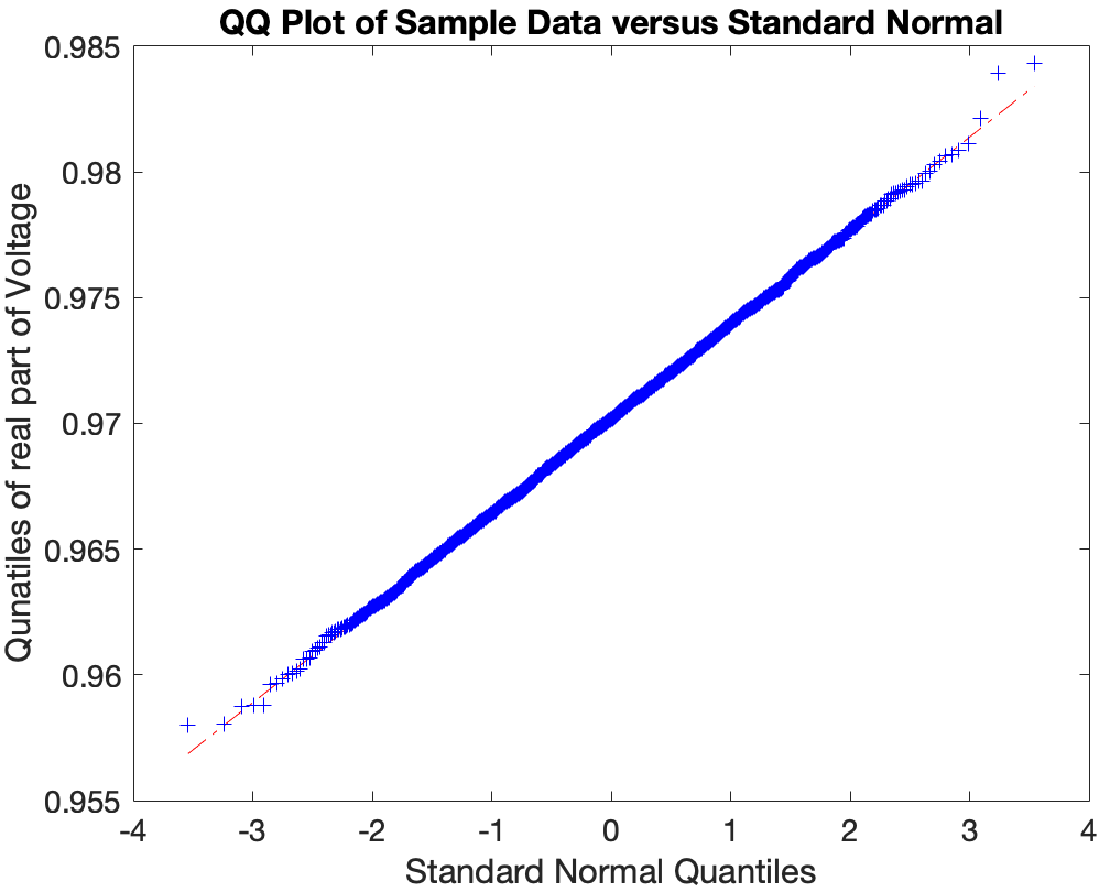
(a)

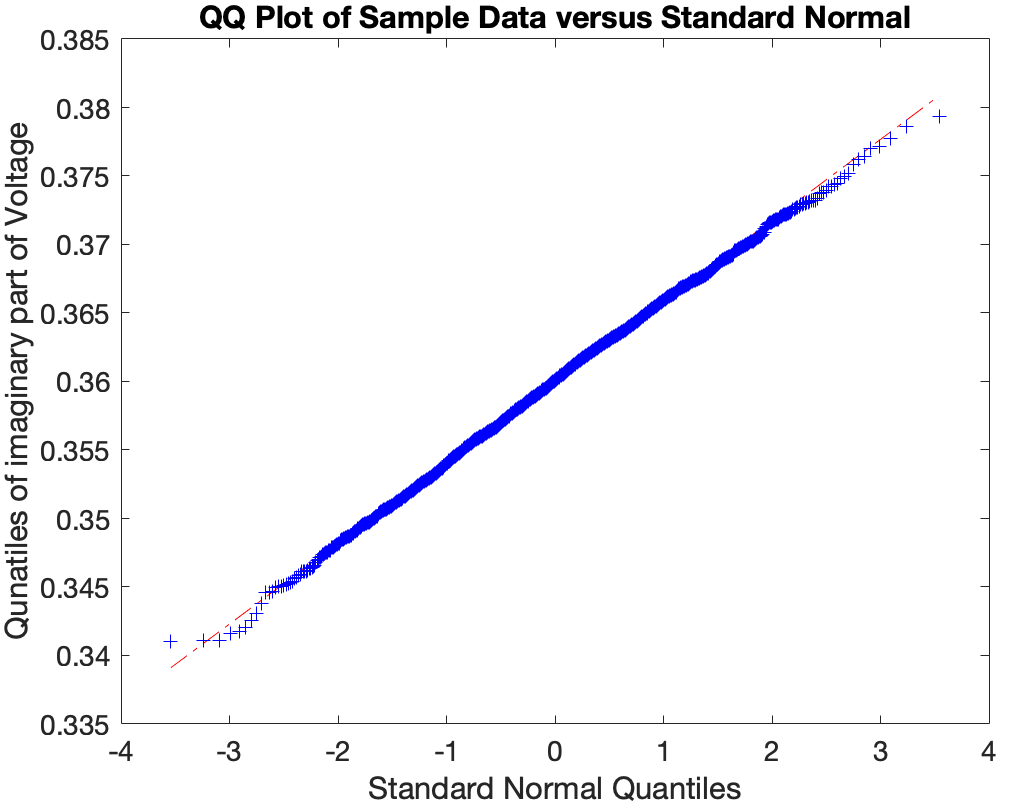
(b)

Figure 2: QQ plot of the (a) real and (b) imaginary part of nodal voltage.

References

- [1] R. A. Jabr, “High-order approximate power flow solutions and circular arithmetic applications,” IEEE Trans. Power Syst., vol. 34, no. 6, pp. 5053–5062, 2019.
- [2] K. Christakou et al., “Voltage control in active distribution networks under uncertainty in the system model: a robust optimization approach,” IEEE Trans. Smart Grid, vol. 9, no. 6, pp. 5631–5642, 2017.
- [3] ——, “Gecn: Primary voltage control for active distribution networks via real-time demand-response,” IEEE Trans. Smart Grid, vol. 5, no. 2, pp. 622–631, 2014.
- [4] R. K. Gupta, F. Sossan, and M. Paolone, “Grid-aware distributed model predictive control of heterogeneous resources in a distribution network: Theory and experimental validation,” IEEE Trans. E. Con., 2020.
- [5] Q. Zhou and J. Bialek, “Simplified calculation of voltage and loss sensitivity factors in distribution networks,” in Proc. 16th Power Syst. Comput. Conf.(PSCC2008), 2008.
- [6] K. Christakou et al., “Efficient computation of sensitivity coefficients of node voltages and line currents in unbalanced radial electrical distribution networks,” IEEE Trans. Smart Grid, vol. 4, no. 2, pp. 741–750, 2013.
- [7] S. Maharjan, A. M. Khambadkone, and J. C.-H. Peng, “Enhanced z-bus method for analytical computation of voltage sensitivities in distribution networks,” IET GTD, vol. 14, no. 16, pp. 3187–3197, 2020.
- [8] C. Mugnier et al., “Model-less/measurement-based computation of voltage sensitivities in unbalanced electrical distribution networks,” in 2016 PSCC. IEEE, 2016, pp. 1–7.
- [9] E. L. da Silva et al., “Data-driven sensitivity coefficients estimation for cooperative control of pv inverters,” IEEE Transactions on Power Delivery, vol. 35, no. 1, pp. 278–287, 2019.
- [10] R. Gupta, F. Sossan, and M. Paolone, “Model-less robust voltage control in active distribution networks using sensitivity coefficients estimated from measurements,” EPSR, vol. 212, p. 108547, 2022.
- [11] R. K. Gupta, “Methods for grid-aware operation and planning of active distribution networks,” p. 247, 2023. [Online]. Available: http://infoscience.epfl.ch/record/299705
- [12] S. Fahmy and M. Paolone, “Analytical computation of power grids’ sensitivity coefficients with voltage-dependent injections,” in 2021 IEEE Madrid PowerTech. IEEE, 2021, pp. 1–6.
- [13] M. Paolone, J.-Y. Le Boudec, S. Sarri, and L. Zanni, “Static and recursive pmu-based state estimation processes for transmission and distribution power grids,” The Institution of Engineering and Technology-IET, Tech. Rep., 2015.
- [14] M. Lefebvre, R. Keeler, R. Sobie, and J. White, “Propagation of errors for matrix inversion,” Nuclear Instruments and Methods in Physics Research Section A: Accelerators, Spectrometers, Detectors and Associated Equipment, vol. 451, no. 2, pp. 520–528, 2000.
- [15] W. H. Kersting, “Radial distribution test feeders,” in 2001 IEEE Power Engineering Society Winter Meeting. Conference Proceedings, vol. 2. IEEE, 2001, pp. 908–912.
- [16] P. Romano and M. Paolone, “Enhanced interpolated-dft for synchrophasor estimation in fpgas: Theory, implementation, and validation of a pmu prototype,” IEEE Transactions on Instrumentation and Measurement, vol. 63, no. 12, pp. 2824–2836, 2014.
- [17] Instrument Transformers:, “Additional requirements for electronic voltage transformers,” Standard IEC, pp. 61 869–8, 2011.