Declassiflow: A Static Analysis for Modeling Non-Speculative Knowledge to Relax Speculative Execution Security Measures (Full Version)

Abstract.

Speculative execution attacks undermine the security of constant-time programming, the standard technique used to prevent microarchitectural side channels in security-sensitive software such as cryptographic code. Constant-time code must therefore also deploy a defense against speculative execution attacks to prevent leakage of secret data stored in memory or the processor registers. Unfortunately, contemporary defenses, such as speculative load hardening (SLH), can only satisfy this strong security guarantee at a very high performance cost.

This paper proposes Declassiflow, a static program analysis and protection framework to efficiently protect constant-time code from speculative leakage. Declassiflow models “attacker knowledge”—data which is inherently transmitted (or, implicitly declassified) by the code’s non-speculative execution—and statically removes protection on such data from points in the program where it is already guaranteed to leak non-speculatively. Overall, Declassiflow ensures that data which never leaks during the non-speculative execution does not leak during speculative execution, but with lower overhead than conservative protections like SLH.

1. Introduction

Security-sensitive programs, such as cryptographic software, perform computations over secret data (e.g., cipher keys and plaintext or personal information). Secure software must prevent its secrets from being “leaked” over microarchitectural side channels, which occur when secret data is passed as the operand to a transmitter instruction. A transmitter is an instruction whose execution creates operand-dependent hardware resource patterns that can potentially be observed (“received”) by the attacker, allowing the attacker to learn information about the transmitter’s operand. Classic examples of transmitters are load and branch instructions, whose execution makes operand-dependent changes to the cache state (flush+, ; last_level_cache_practical, ) and instruction sequence. However, numerous other “variable time” instructions are also considered transmitters (FPU_leaky, ; Mult_leaky, ; practical_doprogramming, ).

Traditionally, the standard technique for preventing secret leakage over microarchitectural side channels is to use constant-time programming (also called data-oblivious programming). Constant-time code performs its computation without passing secret-dependent data as arguments to transmitter instructions (constanttimersa, ; curve25519, ; poly1305, ; pc_model, ; Raccoon, ; FPU_leaky, ).

Unfortunately, the discovery of speculative execution (or Spectre) attacks (spectre, ; ret2spec, ; smother, ; spectre-BHI, ; retbleed, ) undermines the constant-time approach (smother, ; oisa, ; deianpldi, ; SpectreDeclassified, ). The problem is that constant-time guarantees are based on correct execution semantics and may not hold in an illegal mis-speculated execution created by a speculative execution attack. For example, misprediction of a loop branch (oisa, ), function return (deianpldi, ), indirect call (smother, ), and so on can cause the processor to jump to a transmitter with the transmitter’s operand holding secret data, even though the transmitter’s operand would never contain secret data in a correct execution (see Figure 1).

⬇

for (int i = 0; i < NUM_ROUNDS; i++) {

S = AES_Round(S, round_key[i]);

}

Tr(S);

Figure 1. Example of constant-time code breaking due to speculative execution (oisa, ). Misprediction of the loop branch (i < NUM_ROUNDS) can cause an intermediate value of the AES state S to be passed to a transmitter, Tr($\cdot$).

Consequently, constant-time code must additionally deploy a defense against speculative execution attacks. Importantly, this defense must prevent speculative leakage not only of speculatively-accessed data (read from memory under mis-speculation) (stt, ) but also of non-speculatively-accessed data that already exists in processor registers when mis-speculation begins (as in Figure 1). Contemporary defenses can only satisfy this strong security guarantee by blocking speculation of all transmitters, which incurs a high performance cost (SSLH, ; USLH, ). We therefore ask: how can constant-time code be efficiently protected from speculative execution attacks?

We answer this question with Declassiflow, a static program analysis and protection framework that can relax speculative execution defenses. Our approach enforces the security property proposed by Speculative Privacy Tracking (SPT) (spt, ): data that never leaks during non-speculative execution does not leak during speculative execution. This property implies that data which gets implicitly declassified, due to being passed as the operand of a transmitter in the program’s non-speculative execution, does not need to be protected during the program’s speculative execution. This enables the safe removal of protection mechanisms and commensurately lower performance overhead.

Leveraging the SPT security property to reap performance benefits is non-trivial, however. SPT is only able to achieve gains by introducing hardware mechanisms for dynamically tracking non-speculative leakage and disabling protection at run-time. But SPT hardware is not available in current processors and its future adoption status is not clear. In this paper, we leverage the SPT security property purely in software. The resulting approach can be deployed to improve the performance of constant-time code today. Declassiflow can also identify protection relaxations that SPT hardware misses, because Declassiflow is a static program analysis that reasons about all possible program executions, whereas SPT hardware operates only based on the program’s current execution.

In a nutshell, Declassiflow performs program analysis to determine the “attacker’s knowledge” at every edge in the program’s non-speculative control-flow graph, where “attacker knowledge” refers to the data guaranteed to be implicitly declassified (declared non-secret) by the non-speculative execution if said control transfer occurs at run-time. Declassiflow can thus identify data that is guaranteed to leak if execution reaches a program point (although it may not leak at that point, but only later in the execution).

We use Declassiflow’s analysis to relax speculative execution protections, such as SLH, for several constant-time programs. By reasoning about attacker knowledge, Declassiflow is able to deduce that many transmitters (e.g., loads) leak information about the “same thing” (e.g., the base address of an array) and that this information is guaranteed to be known in the program’s non-speculative execution. This enables Declassiflow to reduce overhead significantly; in some cases, replacing all protection instrumentation with a single mechanism (e.g., a barrier) that guarantees the program is entered non-speculatively.

To summarize, we make the following contributions.

1. We propose an abstraction, non-speculative knowledge, for deducing a program region where a variable will “inevitably” be leaked in the program’s non-speculative execution.

2. We propose a novel program analysis that can calculate non-speculative attacker knowledge at each program edge, and strategies for placing protection primitives based on said non-speculative attacker knowledge.

3. We evaluate the impact of our analysis on three constant-time benchmarks and demonstrate that our analysis leads to more efficiently protected programs.

Our analysis is open source, and can be found at https://github.com/FPSG-UIUC/declassiflow.

2. Background

2.1. Programs, Executions, and Traces

2.1.1. The Building Blocks of a Program

We consider programs written in the LLVM assembly language (llvm-lang, ), which uses static single assignment (SSA) (Section 2.2).

A program is a list of instructions that perform computations on variables. $\mathbb{V}$ denotes the set of all variables in the program, and $2^{\mathbb{V}}$ denotes the powerset of $\mathbb{V}$.

Instructions in a program are partitioned into smaller lists, basic blocks (or blocks for short), defined in the usual way. They are typically denoted as $B$, often with a subscript. We use $\mathbb{B}$ to denote the set of all blocks in the program.

A control-flow edge (or edge for short) is an ordered pair $(B_{i},B_{j})$ for some $B_{i},B_{j}\in\mathbb{B}$. A control-flow edge exists between $B_{i}$ and $B_{j}$ if it is theoretically possible to execute $B_{j}$ immediately after $B_{i}$ has been executed. Edges are denoted as $e$, often with a subscript. We use $\mathbb{E}$ to denote the set of all edges in the program. For any block $B$, we denote the set of its input edges and output edges as $E_{\textup{in}}(B)$ and $E_{\textup{out}}(B)$ respectively.

A control-flow graph is a directed graph where the nodes are given by $\mathbb{B}$ and the edges are given by $\mathbb{E}$. We define a node $\textsc{Entry}\in\mathbb{B}$ which is the singular point of entry for the program as well as a node $\textsc{Exit}\in\mathbb{B}$ which is the singular exit point of the program. By definition, $E_{\textup{in}}({\textsc{Entry}})=\varnothing$ and $E_{\textup{out}}({\textsc{Exit}})=\varnothing$.

For any two blocks $B_{i},B_{j}\in\mathbb{B}$, $B_{i}$ dominates $B_{j}$, denoted $B_{i}\,\text{dom}\,B_{j}$, if every path from Entry to $B_{j}$ goes through $B_{i}$. $B_{j}$ post-dominates $B_{i}$, denoted $B_{j}\,\text{pdom}\,B_{i}$, if every path from $B_{i}$ to Exit goes through $B_{j}$. $B_{i}$ is a predecessor of $B_{j}$ if ($B_{i}$, $B_{j}$) $\in\mathbb{E}$.

We say that an edge $e=(B_{i},B_{j})$ dominates a block $B^{\prime}$ if $B_{j}\,\text{dom}\,B^{\prime}$. Similarly, $B^{\prime}$ dominates edge $e$ if $B^{\prime}\,\text{dom}\,B_{i}$. A variable $x$ dominates edge $e$ if the block in which $x$ is defined, denoted as $B_{x}$, dominates $B_{i}$. Similarly, $e$ dominates $x$ if $B_{j}\,\text{dom}\,B_{x}$.

A region, typically denoted $R$, is a set of blocks such that: there is one block in $R$, known as the header, that dominates all others; for any two blocks $B_{i}\in\mathbb{B}$ and $B_{j}\in R$, if there is a path from $B_{i}$ to $B_{j}$ that doesn’t contain the header, then $B_{i}$ is in $R$ (dragon-book, ).

Edge $(B_{i},B_{j})$ is a back edge if $B_{j}\,\text{dom}\,B_{i}$. By convention, every block dominates itself, and so self edges (edges where $B_{i}=B_{j}$) are considered back edges. If there is a back edge in the control-flow graph, then there is a cycle. Cycles in the control-flow graph are typically created by using loop constructs (e.g. for and while).

2.1.2. Executions and Traces

A non-speculative execution of a program $P$ on some input is the sequence of instructions $P$ executes according to the semantics of the LLVM language (llvm-lang, ). We say that the $k$-th instruction in an execution occurs at time $k$. An execution traverses edge $e=(B_{i},B_{j})$ at time $k$ if the $k$-th and $(k+1)$-th instructions are the last instruction in $B_{i}$ and the first instruction in $B_{j}$, respectively.

A trace, typically denoted as $t$, is a sequence of edges. A trace $t$ is realizable if, for some execution of the program, $t$ is the sequence of edges traversed by the execution. Realizable traces thus model the control flow of executions. We refer to them interchangeably for brevity, understanding that every realizable trace is associated with an execution. The set of all realizable traces of the program is denoted $\mathbb{T}$. An edge $e$ is realizable if $e\in t$ for some $t\in\mathbb{T}$.

We use $\mathbb{P}$ to denote all possible paths through the control-flow graph, including those that do not correspond to a realizable trace. By definition, $\mathbb{T}\subseteq\mathbb{P}$.

We now extend our execution semantics to capture speculative executions. We consider control-flow speculation of branches whose speculative target is consistent with the control-flow graph. That is, for $B_{i}\neq B_{j}$, a speculative execution executes instruction $I\in B_{i}$ followed by instruction $I^{\prime}\in B_{j}$ only if $I$ is the last instruction in $B_{i}$, $I^{\prime}$ is the first instruction in $B_{j}$, and $e=(B_{i},B_{j})\in\mathbb{E}$. The semantics of the LLVM assembly language (llvm-lang, ) can be extended to model this form of speculation by adding microarchitectural events for mispredicted control-flow instructions and eventual rollback of a mis-speculated sequence of instructions; this would be similar to various semantics developed in prior work (kopfcontracts, ; Spectector, ; InSpectre, ; blade, ).

The implications of the above speculative semantics on our analysis are discussed in Section 3.

2.2. Single Static-Assignment Form

Our analysis works with code written in single static-assignment (SSA) form. This is a popular and useful abstraction that makes program data dependencies clear and variable identities unambiguous. Code is in SSA form when any usage of a variable is reached by exactly one definition of that variable (ssa, ).

In code with control flow, a variable’s definition may depend on earlier control-flow decisions. In order to make such code SSA-compliant, control flow-dependent definitions at join points are assigned to by -functions (ssa, ) which return an input based on the control-flow decision. We define the semantics of the -function as follows: suppose in some block $B$ we have an instruction $I_{\phi}$ that is a -function, $y=\phi(x_{1},\dots,x_{N})$. By definition, there are $N$ edges into $B$, denoted $e_{1},\dots,e_{N}$. The -function is defined such that at any point in any execution, if $e_{i}$ is the last edge to reach $I_{\phi}$, then $y=x_{i}$. An important consequence of the semantics of a -function is that every $x_{i}$ must be defined prior to $B$. This is simply because it must be a usable name by the time the -function is encountered.

As an example, the following non-SSA code on the left is transformed to produce SSA code on the right.

⬇

x = 0;

if (...) {

x = x + 1

}

print(x)

⬇

x${}_{\text{1}}$ = 0;

if (...) {

x${}_{\text{2}}$ = x${}_{\text{1}}$ + 1

}

x${}_{\text{3}}$ = (x${}_{\text{1}}$,x${}_{\text{2}}$)

print(x${}_{\text{3}}$)

3. Setting and Security Goal

The goal of Declassiflow is to efficiently prevent speculative leakage of sensitive data while maintaining a useful security guarantee.

First and foremost, we define the points of potential information “leakage.” A transmitter is any instruction whose execution exhibits operand-dependent hardware resource usage. Classic examples of transmitters are loads and branches (kocher1996timing, ). Depending on the microarchitecture, there may be others (FPU_leaky, ; pandora, ; practical_doprogramming, ; oisa, ; USLH, ). We say that the operands (data) passed to a transmitter are leaked. Note that a transmitter may leak its operands fully or partially.

A non-speculative transmitter is one that appears in the program’s non-speculative execution. A speculative transmitter appears in the program’s speculative execution. That is, it appears as an operand-dependent microarchitectural event in the program’s speculative semantics (Section 2.1.2), which may or may not correspond to an instruction that architecturally retires.

We assume the standard attacker used in the constant-time programming setting (stt, ; sdo, ; spt, ; blade, ; kopfcontracts, ). Here, the attacker knows the victim program. The attacker further sees a projection, or view, of the victim’s non-speculative and speculative executions: namely, the sequence of values taken by the program counter (PC), and the sequence of values passed to transmitters.

With the above in mind, there are two main protection guarantees a speculative execution defense can have (stt, ). The first prevents speculatively-accessed data from being passed to speculative transmitters. Enforcing this policy satisfies “weak speculative non-interference” (kopfcontracts, ), and is sufficient to eliminate universal read gadgets and defend programs in sandbox settings (spectre_google, ). As a result, there has been significant interest in both hardware (stt, ; sdo, ; spectre_guard, ) and software (slh, ; blade, ) defenses that provide said guarantee.

Unfortunately, such defenses are not comprehensive as there are still important applications—namely constant-time cryptography—that non-speculatively read and compute on sensitive data but can still leak said data speculatively (spt, ; kopfcontracts, ; stt, ; NDA, ; dolma, ). To protect these programs, one requires a defense with a broader protection guarantee: i.e., one that prevents both speculatively and non-speculatively accessed data from being passed to speculative transmitters. Defense mechanisms that meet this guarantee provide complete protection from speculative execution attacks but typically come at high performance overhead, i.e., they are tantamount to delaying every transmitter’s execution until they become non-speculative or are squashed (NDA, ; SSLH, ; USLH, ).

The aforementioned protections are (almost always) overly conservative because they implicitly treat all data as “secret” and deserving of protection. Yet, not all data is semantically secret. Software annotations could directly convey what is and is not secret, but there are major disadvantages to programmer intervention. For example, programmer intervention/expert labeling cannot be applied to legacy code already deployed. So, to determine what data is secret without requiring expert labeling/intervention, we adopt a definition of “secret” proposed by SPT (spt, ),

Definition 0.

Data $x$ is secret if there is no data flow from it to an operand of a non-speculative transmitter, where data flow refers to flow through LLVM SSA variables and LLVM data memory.

This definition is motivated by the constant-time programming model in which sensitive data is never passed to non-speculative transmitters. The contrapositive of this is that if any data is passed to a non-speculative transmitter, it is not sensitive, i.e. not “secret”.

Definition 1 can be interpreted as enabling efficient implementations that satisfy generalized constant-time (GCT) (kopfcontracts, ). Denote the non-speculative and speculative program semantics as $S^{\mathsf{nspec}}$ and $S^{\mathsf{spec}}$, respectively. For brevity, we also assume these semantics encode the attacker’s view, e.g., the set of transmitters. Given, a program $P$ and a policy $\Pi$ which defines what program variables are “high” (secret), $P$ satisfies GCT w.r.t. $S^{\mathsf{nspec}}$, $S^{\mathsf{spec}}$ and $\Pi$ if the following requirements hold.

1. Executions of $P$ on $S^{\mathsf{nspec}}$ satisfy non-interference w.r.t. $\Pi$. That is, attacker observations of $P$’s execution, given $S^{\mathsf{nspec}}$, are independent of the values in $\Pi$.

2. Executions of $P$ on $S^{\mathsf{nspec}}$ that satisfy non-interference w.r.t. $\Pi$ must also satisfy non-interference on $S^{\mathsf{spec}}$ w.r.t. $\Pi$.

Requirement 2 is referred to as speculative non-interference or SNI for short (kopfcontracts, ; Spectector, ).

Given this context, we can view Declassiflow as a function $P^{\prime}=D(P;S^{\mathsf{nspec}},S^{\mathsf{spec}})$ that takes a program $P$ as input, produces a program $P^{\prime}$ as output, and is parameterized by $S^{\mathsf{nspec}}$ and $S^{\mathsf{spec}}$. Suppose $P$ satisfies Requirement 1; it need not satisfy Requirement 2. For a specified $S^{\mathsf{nspec}}$ and $S^{\mathsf{spec}}$, $D$ outputs a $P^{\prime}$ that is functionally equivalent to $P$ and now (additionally) satisfies Requirement 2, i.e., now satisfies SNI and therefore GCT.

Importantly, $D$ did not require $\Pi$ as an input, but rather infers a policy $\Pi_{\text{\scriptsize Decl}}$ which is sound w.r.t. $\Pi$. That is, $\Pi\subseteq\Pi_{\text{\scriptsize Decl}}$. This is possible because $D$ has access to $P$, which already enforces $\Pi$. At the same time, $\Pi_{\text{\scriptsize Decl}}$ will provide a basis for implementing efficient protection. That is, if $\Pi_{\text{\scriptsize{All}}}$ denotes the policy (described above) that treats all data as secret, we have that $\Pi_{\text{\scriptsize Decl}}\subseteq\Pi_{\text{\scriptsize{All}}}$ in theory and $\Pi_{\text{\scriptsize Decl}}\subset\Pi_{\text{\scriptsize{All}}}$ in practice. This will allow us to more efficiently protect programs without additional programmer intervention or labeling, beyond the program being written to enforce non-speculative/vanilla constant-time execution.

3.1. Semantics and Transmitters

$D$ is parameterized by $S^{\mathsf{nspec}}$ and $S^{\mathsf{spec}}$, which encode the execution semantics and transmitters.

Semantics

For security, our analysis assumes the semantics set forth in Section 2.1.2, in particular that the speculative semantics is restricted to control-flow speculation that remains on the control-flow graph. This is sufficient to protect non-speculatively accessed data in the presence of direct branches (similar to those found in Spectre Variant 1). To block leakage due to other forms of speculation (e.g., indirect branches whose targets are predicted, as in Spectre variant 2), our analysis can adopt complementary defenses such as “retpoline”.

Transmitters

Our analysis is flexible with respect to which instructions are considered transmitters. For the rest of the paper, we assume loads are transmitters that can execute speculatively. We assume that branches and stores are also transmitters, but only if they appear in the non-speculative execution. That is, we assume that branches and stores do not change microarchitectural state in an operand-dependent way until they become non-speculative. We note, this still allows for branch prediction; it just stipulates that said predicted branches only resolve (and redirect execution) when they become non-speculative. To reiterate: these choices were not fundamental, and the analysis can be modified to account for other transmitters and their speculative vs. non-speculative behavior.

4. Achieving Efficient Protection

We now describe an analysis, dubbed Declassiflow, that enables low-overhead protection for “secrets” as given by Definition 1.

To understand our scheme’s security and performance, we start by considering a secure but high-overhead software-based protection. We will use the abstraction proposed by Blade (blade, ), which introduces a primitive called protect(v). protect wraps a variable v and delays its usage until it becomes non-speculative (or stable (blade, )). Blade points out that, while current hardware does not support protect, protect can be emulated today by introducing control-flow-dependent data dependencies (slh, ), speculation barriers, or a combination of the two. Regardless of how it is implemented, executing protect incurs overhead by delaying an instruction’s (and its dependents’) execution. This is especially pronounced when said instruction is on the critical path for instruction retirement (as is typical with loads).

As discussed in Section 3, we wish to protect non-speculatively accessed data. Thus, a secure baseline defense must protect the operands of all transmitters that can execute speculatively. We express this by wrapping said transmitters’ operands with protect statements, placed immediately before each transmitter and in the same block. This approach is tantamount to that of several recent defense proposals (SSLH, ; USLH, ; NDA, ).

An example of our baseline is shown in Figure LABEL:fig:motiv-example-orig, which depicts a program that contains a transmitter inside a loop as well as at the exit point. The transmitters are denoted Tr($\cdot$). While this approach is secure, it is also expensive; the protect(x) statements can be encountered an unbounded number of times (depending on the semantics of the loop). Given this strict policy, which effectively prevents transmitters from executing speculatively, nothing more can be done to improve performance in this example.

However, if we instead consider Definition 1 and its implications, we can see that this program contains unnecessary protection. From the discussion surrounding that definition, we saw that data which does not meet the definition for “secret” does not need to be protected from speculative leakage. This is the manner in which we can reduce protection overhead. To aid in this process, we define a more useful concept that is core to our work,

Definition 0.

A variable $x$ is considered known when it is guaranteed to be passed to a non-speculative transmitter (i.e., its value will inherently be revealed) or when its value can be inferred from other known variables.

We say that a variable can be “inferred” from other known variables if its value can be computed via a polynomial-time algorithm from the values of said other variables. We consider the set of known variables over time to be the attacker’s non-speculative knowledge (or just “knowledge” for short). One key addition made by Definition 1 is that a variable can be considered known not only when it is observed to be non-secret, but even when it is guaranteed to eventually become non-secret. That is, for the purposes of our analysis, inevitable non-secrecy is as good as knowledge.

Our goal is to use Definition 1 to derive a minimal set of locations at which to place protect statements. For this, we need to define one more concept: the non-speculative knowledge frontier (knowledge frontier for short) for each program variable. Intuitively, the knowledge frontier for a variable $x$ represents the earliest points in the program such that, if the program’s non-speculative execution “crosses” the knowledge frontier, $x$ will be known. We define it more precisely as,

Definition 0.

For any variable $x$, let $K_{\mathbb{B}}(x)$ denote the set of blocks in which $x$ is known. The knowledge frontier of $x$, denoted $\mathcal{F}(x)$, is the smallest subset of $K_{\mathbb{B}}(x)$ such that for any $B$ in $K_{\mathbb{B}}(x)$, there is no path from Entry to $B$ that does not contain some $B^{\prime}$ from $\mathcal{F}(x)$.

Note that by this definition, the knowledge frontier for a variable in a given program is unique. We can reframe what is required of a protection mechanism to enforce SNI (with respect to the policy implied by Definition 1) in terms of the knowledge frontier,

Property 1.

(Frontier Protection Property for $x$) A placement of protect(x) statements enforces SNI with respect to $x$ if and only if no speculative execution can transmit a function of $x$ before the non-speculative execution crosses the knowledge frontier for $x$.

One straightforward strategy to satisfy Property 1 is to add protect statements only “along the knowledge frontier” for each given variable, as opposed to at the site of each transmitter.

Example

Look again at the program in Figure 2. As mentioned, a naive protection scheme places protect(x) statements in the same blocks as all transmitters. However, if the execution enters $B_{1}$ non-speculatively, it will necessarily (non-speculatively) enter either $B_{2}$ or $B_{3}$ next. Thus, the knowledge frontier for x is $B_{1}$. With this, we can re-instrument the code with a protect(x) inserted in $B_{1}$ only. Crucially, we have removed the protect(x) from the loop, which means that protection overhead will likely be amortized.

This is more aggressive than what is possible with the hardware-based defense SPT, on which Definition 1 is based. Since SPT doesn’t know the program’s structure, it doesn’t know if there is a path from $B_{1}$ where x is not leaked non-speculatively, and hence it falls back to a baseline protection that is tantamount to Figure LABEL:fig:motiv-example-orig. As mentioned, an interesting aspect of Definition 1 is that it allows for variables to be known “ahead of time” (i.e. before they are actually passed to a transmitter). This is a key difference between our approach and SPT’s; knowledge that is inevitable in the future is knowledge that can be exploited “now.” SPT on the other hand must wait to observe transmitters retire before it treats its operands as known.

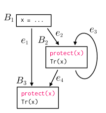
(a)

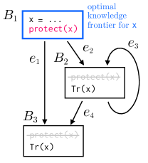
(b)

Figure 2. Making the protected code (left) more efficient (right).

5. Modeling Attacker Knowledge

We will now define non-speculative attacker knowledge, which will be used to compute the non-speculative knowledge frontier.

5.1. Non-Speculative Knowledge

We model the attacker’s knowledge at the granularity of variables, and we treat knowledge in a binary fashion; the value of a variable is either “fully” known to an attacker or no function of the variable is known. Thus, an attacker’s knowledge is a subset of $\mathbb{V}$, and the full space of the knowledge of an attacker is $2^{\mathbb{V}}$.

Per Definition 1, in any trace, a variable is considered known at the point when (and any time after) it is passed to a non-speculative transmitter (i.e., when its value is revealed), or at the point (and any time after) its value can be inferred from other known variables. Rather than keeping track of knowledge “temporally” by tracking it over time (per trace), we can instead capture knowledge “spatially” by mapping it onto the control-flow graph. We introduce the map ${K_{\mathbb{E}}}:\mathbb{E}\to 2^{\mathbb{V}}$ which represents the distribution of knowledge over edges. We precisely define ${K_{\mathbb{E}}}$ as follows,

Definition 0.

Take any edge $e\in\mathbb{E}$. We have $x\in{K_{\mathbb{E}}}(e)$ if and only if for all traces $t\in\mathbb{T}$ such that $e\in t$, $x$ is already known or is guaranteed to become known every time the execution corresponding to $t$ traverses $e$. If $x\in{K_{\mathbb{E}}}(e)$, we say “$x$ is known on edge $e$”.

There are two important clarifications we wish to make with respect to the above definition. First and foremost, $x\in{K_{\mathbb{E}}}(e)$ does not necessitate that $e$ is dominated by the definition of $x$ since the value of $x$ may be inferable from other known variables, as discussed above. Second, the manner in which we define knowledge and the way we intend to use it leave open the possibility for vacuous knowledge. A variable is vacuously known if it is deduced to be known on a path on which it will never be defined. Crucially, since such a variable is not defined on this path, it cannot be used. Thus, for the purposes of optimizing a defense mechanism, this knowledge is inactionable. We will see in the next section that vacuous knowledge is an important concept, particularly when analyzing -functions.

5.2. Instructions as Equations

We now define a set of relations that describe knowledge ${K_{\mathbb{E}}}$ with respect to a concrete program.

5.2.1. Non- instructions

We first discuss how knowledge is propagated through non- instructions. An instruction $I$ is said to be deterministic if it can be represented as an equation of the form $y=f(x_{1},\dots,x_{N})$. Control-flow instructions, by convention, don’t have an output. Loads and stores are not considered deterministic since our current analysis does not model the contents of memory. We define $\text{out}(I)=y$ and $\text{in}(I)=\{x_{1},\dots,x_{N}\}$.

Deterministic instructions are of interest since knowing all but one of their operands/results enables deduction of the remaining one. We say an instruction $I$ is forward solvable if, for all concrete assignments to $x_{i}\in\text{in}(I)$, we have a unique solution for $y$. We say $I$ is backward solvable if for any $x_{i}\in\text{in}(I)$, for all concrete assignments to $\text{out}(I)$ and all $x_{i\neq j}\in\text{in}(I)$, we have a unique solution for $x_{i}$. All deterministic instructions (e.g., add, sub, mul) are forward solvable; not all are backwards solvable. Exploiting the solvability of instructions is how we achieve propagation of knowledge through computations as motivated in Section 4.

An important consequence of working with programs expressed in SSA form is that the equations that define variables are unique. Crucially (and perhaps counter-intuitively) this implies the equations associated with instructions are exploitable anywhere in the control-flow graph, even if the associated instruction is not encountered in a given trace or is unreachable in general. When analyzing a non SSA-form program, there may be multiple definitions for any given variable, and thus you need to consider only the definitions that apply to the locale you are in. Attempting to analyze a non-SSA program while keeping track of which definitions apply where implicitly converts the program to SSA form. We will see the benefits of the global view of equations in the examples from Section 5.3.

5.2.2. -functions

We now discuss -functions. Before we begin, recall that the PC is public to the attacker due to assumptions made by the constant-time programming model (Section 3). Since the PC is public, it can be considered known at all points in time in the non-speculative execution.

Because the PC is known, we can treat -functions as being forward solvable. If at any point all of a -function’s inputs are known, then regardless of which one gets assigned to the output, the output must be known as well. Consider a -function $I_{\phi}$ of the form $y=\phi(x_{1},\dots,x_{N})$ in a block $B$ with input edges $e_{i}$ and output edges $e_{o}$. The semantics of $I_{\phi}$ are such that $y=x_{i}$ if $e_{i}$ is taken to reach $B$. Now, suppose that $x_{1},\dots,x_{N}$, are known on some edge $e$. If $e$ is in a trace containing $I_{\phi}$, we know $y$ because we know which $x_{i}$ is assigned to $y$ (because the PC is known) and we know each $x_{i}$. Note that if $I_{\phi}$ is not in a trace containing $e$, then knowledge of $y$ is vacuous; it cannot be used in a meaningful way.

There is an additional, more subtle version of forward solvability when considering -functions. Consider again $I_{\phi}$ as defined before. If each input $x_{i}$ to the -function is known on its respective edge $e_{i}$, $y$ is known on all $e_{o}$. This is again due to the assumption that the PC is known; the input edge used to arrive at $B$ is known and thus we will know which $x_{i}$ is assigned to $y$.

Note that -functions are not backward solvable; knowing the output and all but one of the inputs doesn’t necessarily reveal the last input. That said, there is a causal relationship we can exploit in the backwards direction. Using the definition/semantics of $I_{\phi}$ from before, suppose that $y$ is known on all output edges $e_{o}$. Then every $x_{i}$ is known on its respective edge $e_{i}$. The justification is as follows: suppose $e_{i}$ is traversed. Then $y=x_{i}$ and we know for which $x_{i}$ this holds. Now, we must leave $B$ through some $e_{o}$, and $y$ is known on every $e_{o}$. Thus, in this scenario, $x_{i}$ is known.

5.2.3. Knowledge propagation theorems

We summarize the previous discussion with a series of theorems that describe relationships on knowledge. The proofs of these theorems can be found in Appendix A. We start with theorems that describe the knowledge available to every edge in isolation,

Theorem 2.

Consider an instruction $I$ of the form Tr(x) in some block $B$ with output edges $e_{o}$. For all $e_{o}$, $x\in{K_{\mathbb{E}}}(e_{o})$.

Theorem 3.

Take any edge $e\in\mathbb{E}$. Consider a forward solvable instruction $I$ from anywhere in the control-flow graph, and suppose it is of the form $y=f(x_{1},\dots,x_{N})$. If $x_{i}\in{K_{\mathbb{E}}}(e)$ for all $x_{i}$, then $y\in{K_{\mathbb{E}}}(e)$.

Theorem 4.

Take any edge $e\in\mathbb{E}$. Consider a backward solvable instruction $I$ from anywhere in the control-flow graph, and suppose it is of the form $y=f(x_{1},\dots,x_{N})$. For any $j\in\{{1,\dots,N}\}$, suppose we have all $x_{i\neq j}\in{K_{\mathbb{E}}}(e)$ as well as $y\in{K_{\mathbb{E}}}(e)$. Then $x_{j}\in{K_{\mathbb{E}}}(e)$.

The following theorems describe the relationship of knowledge between edges in the general case,

Theorem 5.

Consider a block $B$. If for some variable $v$ we have $v\in\bigcap{K_{\mathbb{E}}}(e_{i})$ for all realizable $e_{i}$ in $E_{\textup{in}}(B)$, then we have $v\in{K_{\mathbb{E}}}(e_{o})$ for every $e_{o}\in E_{\textup{out}}(B)$.

Theorem 6.

Consider a block $B$. If for some variable $v$ we have $v\in\bigcap{K_{\mathbb{E}}}(e_{o})$ for all realizable $e_{o}$ in $E_{\textup{out}}(B)$, and if $v$ is not defined in $B$, then we have $v\in{K_{\mathbb{E}}}(e_{i})$ for every $e_{i}\in E_{\textup{in}}(B)$.

An important thing to notice about Theorem 6 is that we mandate $v$ is not defined in $B$. This is because if $v$ is not defined in $B$, then nothing in $B$ can change $v$’s status in terms of knowledge; this is not true if $v$ is defined in $B$. That said, the theorem does not prevent variables from being known prior to their definition; they just need to be inferable (via the other theorems).

The following theorems describe the relationship of knowledge between edges in the special case that they are connected via a -function.

Theorem 7.

Let $I_{\phi}$ denote a -function of the form $y=\allowbreak\phi(x_{1},\allowbreak\dots,\allowbreak x_{N})$ in block $B$ with $N$ input edges $e_{1},\dots,e_{N}$. The semantics of $I_{\phi}$ are such that $y=x_{i}$ if $e_{i}\in E_{\textup{in}}(B)$ is traversed to reach $B$. If for all realizable $e_{i}$ we have $x_{i}\in{K_{\mathbb{E}}}(e_{i})$, then for every output edge $e^{\prime}$, $y\in{K_{\mathbb{E}}}({e^{\prime}})$.

Theorem 8.

Let $I_{\phi}$ denote a -function of the form $y=\allowbreak\phi(x_{1},\allowbreak\dots,\allowbreak x_{N})$ in a block $B$ with input edges $e_{1},\dots,e_{N}$. The semantics of $I_{\phi}$ are the same as in Theorem 7. If for all realizable output edges $e^{\prime}$ we have $y\in{K_{\mathbb{E}}}({e^{\prime}})$, then for every $e_{i}$ we have $x_{i}\in{K_{\mathbb{E}}}(e_{i})$.

Note that for Theorems 2–4, the realizability of an edge is not important to our model of knowledge. This is because the claims are about the local knowledge associated with each edge individually, and unrealizable edges only contain vacuous knowledge. On the other hand, Theorems 5–8 make use of the realizability of edges since we are considering the relationships between edges.

5.3. Examples Computing Knowledge/Frontiers

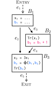
(a)

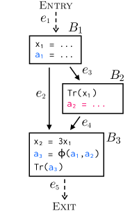
(b)

Figure 3. Examples used to illustrate knowledge over edges (${K_{\mathbb{E}}}$).

Figure 3 shows an example of how to compute knowledge (and then the knowledge frontier) with the relations from Section 5.2.

First consider Figure LABEL:fig:program-B. There are two paths through the control-flow graph; we’ll assume they both correspond to realizable traces. Starting off, we have Tr(b${}_{\text{3}}$) in $B_{3}$ which leads to knowing $b_{3}$ on edge $e_{5}$ (Theorem 2) and subsequently $b_{1}$ on $e_{2}$ and $b_{2}$ on $e_{4}$ (Theorem 8). The equation $b_{2}=b_{1}+1$ and Theorem 3 enable us to deduce $b_{2}$ everywhere $b_{1}$ is known (and vice versa by Theorem 4)—similarly for $x_{1}$, $x_{2}$ and $x_{2}=3x_{1}$. Since both $b_{1}$ and $b_{2}$ are known on $e_{2}$, $e_{3}$, and $e_{4}$, by Theorem 3, $b_{3}$ is also known on $e_{2}$, $e_{3}$, and $e_{4}$.

By continuing to apply the theorems, we get ${K_{\mathbb{E}}}(e_{1})=\varnothing$, ${K_{\mathbb{E}}}(e_{2})=\{{b_{1},b_{2},b_{3}}\}$, ${K_{\mathbb{E}}}(e_{3})={K_{\mathbb{E}}}(e_{4})=\{{b_{1},b_{2},b_{3},x_{1},x_{2}}\}$, and ${K_{\mathbb{E}}}(e_{5})=\{{b_{1},b_{2},b_{3}}\}$.

This provides a basis for the frontier of $x_{1}$ and $x_{2}$ to be $\{{B_{2}}\}$. More importantly, it means the frontier for $b_{1},b_{2},b_{3}$ is $\{B_{1}\}$. A program that non-speculatively enters $B_{1}$ will inherently transmit all three. (We detail more precisely how to compute the frontier given ${K_{\mathbb{E}}}$ in Section 6.3.) This will enable more efficient protection: to enforce Property 1, it is sufficient to add protect statements for $b_{1},b_{2},b_{3}$ solely in $B_{1}$.

Next consider Figure LABEL:fig:program-A, which is almost the same as Figure LABEL:fig:program-B except for two changes: first, every $b_{i}$ is replaced with $a_{i}$ for clarity; second (and most importantly), the equations for $a_{2}$ and $b_{2}$ differ. We use a${}_{\text{2}}$ =$\;\dots$ to represent a non-deterministic instruction. Since we no longer have an equation relating $a_{2}$ to $a_{1}$ (as we did with $b_{2}=b_{1}+1$ from before), the knowledge settles to ${K_{\mathbb{E}}}(e_{1})=\varnothing$, ${K_{\mathbb{E}}}(e_{2})=\{{a_{1}}\}$, ${K_{\mathbb{E}}}(e_{3})={K_{\mathbb{E}}}(e_{4})=\{{x_{1},x_{2},a_{2}}\}$, and ${K_{\mathbb{E}}}(e_{5})=\{{a_{3}}\}$. From this we can deduce that the frontier for $a_{1}$ is $\varnothing$; the frontier for $x_{1}$, $x_{2}$ and $a_{2}$ is $\{{B_{2}}\}$; the frontier for $a_{3}$ is $\{{B_{3}}\}$. This matches our security goal: it is unsafe to hoist protect statements above any variable’s definition because knowing $a_{1}$ is not the same as knowing $a_{2}$ and hoisting a protect would enable an attacker to selectively learn both through Tr(a${}_{\text{3}}$).

5.4. Approximating Non-Speculative Knowledge

⬇

if (q) {

Tr(x)

}

if (!q) {

 Tr(x)

}

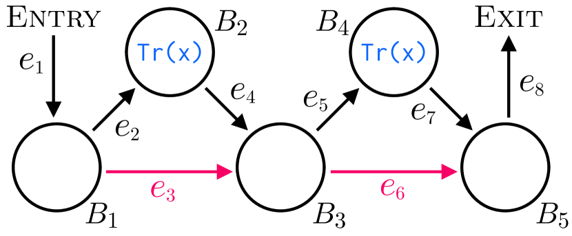
Figure 4. A program and its control-flow graph. The branches are anti-correlated, thus the trace $\{e_{1},{\color[rgb]{0.96875,0,0.40234375}e_{3}},{\color[rgb]{0.96875,0,0.40234375}e_{6}},e_{8}\}$ is not realizable.

Precisely computing ${K_{\mathbb{E}}}$ using the theorems from the previous section is generally intractable since it relies on knowing whether any given edge is realizable. We can instead attempt to compute an approximation of ${K_{\mathbb{E}}}$, denoted as ${\widehat{K}_{\mathbb{E}}}$. We consider our approximation sound if it does not over-estimate an attacker’s true knowledge; we consider it imprecise if it under-estimates it. To compute ${\widehat{K}_{\mathbb{E}}}$, we make the assumption that any path through the control-flow graph corresponds to a realizable trace. More specifically, for any edge $e=(B_{i},B_{j})$, we assume that any edge $e^{\prime}\in E_{\textup{in}}(B_{i})$ may have been traversed prior to it, and any edge $e^{\prime\prime}\in E_{\textup{out}}(B_{j})$ may be traversed after it. Looking back at Definition 1, by increasing the number of traces we consider $e$ to have been part of, we are (potentially) reducing the size of ${{\widehat{K}_{\mathbb{E}}}(e)}$; i.e. ${{\widehat{K}_{\mathbb{E}}}(e)}\subseteq{K_{\mathbb{E}}}(e)$. Thus, this approximation method (potentially) loses precision, but it maintains soundness.

Example

Look at Figure 4. The only possible traces are $t_{1}=\{{e_{1},e_{2},e_{4},{\color[rgb]{0.96875,0,0.40234375}e_{6}},e_{8}}\}$ and $t_{2}=\{{e_{1},{\color[rgb]{0.96875,0,0.40234375}e_{3}},e_{5},e_{7},e_{8}}\}$. (We’ve colored edges ${\color[rgb]{0.96875,0,0.40234375}e_{3}}$ and ${\color[rgb]{0.96875,0,0.40234375}e_{6}}$ to correspond with the figure.) The paths $\{\allowbreak e_{1},\allowbreak{\color[rgb]{0.96875,0,0.40234375}e_{3}},\allowbreak{\color[rgb]{0.96875,0,0.40234375}e_{6}},\allowbreak e_{8}\}$ and $\{\allowbreak e_{1},\allowbreak e_{2},\allowbreak e_{4},\allowbreak e_{5},\allowbreak e_{7},\allowbreak e_{8}\}$ do not correspond to realizable traces since they imply q is both true and false. Ideally then, we must have that $x$ is known on $e_{3}$, i.e. ${K_{\mathbb{E}}}({{\color[rgb]{0.96875,0,0.40234375}e_{3}}})=\{{x}\}$, since at this point the execution must take $e_{5}$ and encounter Tr(x). Making the simplifying assumption (above) to compute ${{\widehat{K}_{\mathbb{E}}}(e)}$, however, we cannot assume whether we will take $e_{2}$ vs. ${\color[rgb]{0.96875,0,0.40234375}e_{3}}$; nor can we assume that we will take $e_{5}$ vs. ${\color[rgb]{0.96875,0,0.40234375}e_{6}}$ (for whichever of $e_{2}$ or ${\color[rgb]{0.96875,0,0.40234375}e_{3}}$ we took). In other words, the analysis cannot conclude whether we will encounter Tr(x) and thus deduces that $x$ is not known on ${\color[rgb]{0.96875,0,0.40234375}e_{3}}$; i.e. ${{\widehat{K}_{\mathbb{E}}}({\color[rgb]{0.96875,0,0.40234375}e_{3}})}=\varnothing$. See that ${{\widehat{K}_{\mathbb{E}}}({\color[rgb]{0.96875,0,0.40234375}e_{3}})}\subset{K_{\mathbb{E}}}({{\color[rgb]{0.96875,0,0.40234375}e_{3}}})$; we’ve lost precision in order to gain tractability, but we have not sacrificed soundness.

6. Declassiflow Approaches

In this section, we describe the approach used by Declassiflow to compute and utilize non-speculative attacker knowledge.

At a high level, our analysis first computes ${{\widehat{K}_{\mathbb{E}}}(e)}$ for efficiency reasons (Section 6.1), but invokes more sophisticated analyses to compute ${K_{\mathbb{E}}}(e)$ on specific edges when doing so is deemed profitable (Section 6.2). Later subsections then detail how to use the edge-based knowledge to compute the knowledge frontier (Section 6.3) and instrument protection (Section 6.4). Section 7 goes over lower-level details of all of the above.

6.1. Computing Knowledge via a Data-Flow Analysis

Our ideas from Section 5 map naturally to a data-flow analysis (dragon-book, ).

Data-flow analyses work by assigning data-flow values to every point in the control-flow graph. They iteratively apply local rules known as the data-flow equations to build up and combine these data-flow values. When this process has converged (i.e. the size of the data-flow values stagnates), what remains is a data-flow solution.

A data-flow analysis makes the assumption that any path through the control-flow graph is a potential path the execution may take; it approximates $\mathbb{T}$ with $\mathbb{P}$. Since the definition of ${\widehat{K}_{\mathbb{E}}}$ relies on the same assumption, we can formulate a data-flow analysis such that the solution is exactly ${\widehat{K}_{\mathbb{E}}}$. The specific data-flow equations we use are discussed in Section 7.1. By construction, the result of our ideas applied to Figure 4 (as discussed in Section 5.4) is precisely what our data-flow analysis would yield.

6.2. Improving Precision via Symbolic Execution

There are of course drawbacks to approximating ${K_{\mathbb{E}}}$ as done by the data-flow analysis (see Section 5.4). Namely, under-estimating an attacker’s knowledge causes us to over-estimate the amount of protection needed. To avoid this, we need a way to analyze programs in a way that can deduce whether a trace is unrealizable.

To that end, we also selectively employ symbolic execution (symex-survey, ). In a nutshell, symbolic execution involves executing a program with “symbolic” values; variables are mapped to symbolic expressions rather than concrete values (at least, in the cases when the concrete value cannot be deduced unambiguously). Expressions associated with all variables are derived by the instructions encountered during the symbolic execution. Upon reaching a branch, a symbolic execution engine will traverse both paths separately. Every path through will have associated with it “path constraints”, which are a set of symbolic expressions implied by the set of taken branches.

Our framework uses symbolic execution to answer the following question,

Question 1.

Given some region $R$ of the control-flow graph and given some variable $x$, does there exist a path through $R$ (that corresponds to a realizable trace) upon which $x$ is not transmitted?

Recall that a data-flow analysis conservatively answers this question by assuming that if a path exists, it is part of a realizable trace. By considering the semantics of the instructions and the branch conditions, symbolic execution can try and answer the question less conservatively; though we stress that it does so in a sound manner since it needs to prove that the path cannot be taken.

We can look back at Figure 4 to see how symbolic execution can succeed where the data-flow analysis fails. The candidate region we consider is the entirety of the program. Recall that the problematic path was $p^{\prime}=\{e_{1},{\color[rgb]{0.96875,0,0.40234375}e_{3}},{\color[rgb]{0.96875,0,0.40234375}e_{6}},e_{8}\}$, which again does not correspond to a realizable trace. When the tool considers the path $p^{\prime}$, the path constraints will contain both $q=\text{false}$ and $q\neq\text{false}$. These contradictory statements mean that no non-speculative execution could ever traverse such a path. Thus, symbolic execution will conclude that Tr(x) is unavoidable (i.e. that the answer to Question 1 is “no” for this region and variable $x$) meaning $x$ is guaranteed knowledge at (among other places) the program’s entry point. Thus, we have achieved a more precise result than the data-flow analysis.

The details of how and when we utilize symbolic execution to answer Question 1 are given in Section 7.2.

Note that the symbolic execution cannot be used on its own; the results of the data-flow analysis are a prerequisite. For symbolic execution to work, we will need to instrument the code to indicate what variables are known at various points, and the data-flow analysis is precisely what provides this information. While it is certainly possible to formulate the entire analysis in terms of symbolic execution, this would certainly not scale to larger programs as well as a data-flow analysis would.

6.3. Computing the Knowledge Frontier

As discussed in Section 4, Property 1 is the key to finding a minimal yet sufficient set of protect statements needed to secure a program. To that end, we need to compute the knowledge frontier given the results of the data-flow analysis and/or symbolic execution.

The first step to computing the knowledge frontier is to map knowledge from edges to basic blocks; we want the map ${{\widehat{K}}_{\mathbb{B}}}:\mathbb{B}\to 2^{\mathbb{V}}$. For any block $B$, we define ${{\widehat{K}}_{\mathbb{B}}}\quantity(Bmissing)=\bigcap{{\widehat{K}_{\mathbb{E}}}(e^{\prime})}$ for all $e^{\prime}\in E_{\textup{out}}(B)$. Recall that ${\widehat{K}_{\mathbb{E}}}$ is the result of the data-flow analysis. The results from the symbolic execution constitute additions to ${{\widehat{K}}_{\mathbb{B}}}$. Question 1 is associated with some candidate variable $x$ and some candidate region $R$ of the control-flow graph. If, when given these, the symbolic execution tool answers “no” to Question 1, then $x\in{{\widehat{K}}_{\mathbb{B}}}\quantity(Bmissing)$ for all $B\in R$.

With ${{\widehat{K}}_{\mathbb{B}}}$ in hand, we can compute the frontiers for all variables. For any variable $x$, we first over-estimate $\mathcal{F}(x)$ by adding all $B\in\mathbb{B}$ such that $x\in{{\widehat{K}}_{\mathbb{B}}}\quantity(Bmissing)$. Then, for any $B\in\mathcal{F}(x)$, if $x$ is known in all of $B$’s predecessor blocks, we remove $B$ from $\mathcal{F}(x)$. This is done using another data-flow analysis. After this, $\mathcal{F}(x)$ represents the precise knowledge frontier for $x$.

Consider an arbitrary program function f. For any variable $x$, if its frontier $\mathcal{F}(x)$ is the entry block of f, we say $x$ is fully declassified. If all variables transmitted by f are fully declassified, then f itself is fully declassified.

6.4. Adding Protection

Once we have the knowledge frontier $\mathcal{F}$, we can place protection using a simple strategy: for every variable $x$ that is transmitted, we place protect(x) statements all along its frontier $\mathcal{F}(x)$. We refer to this approach as “enforcing the knowledge frontier”. This is a straightforward method to satisfy Property 1. In terms of hoisting protect statements as high as possible, it is also optimal.

For simplicity, we perform our analysis at the granularity of functions. To that end, we now discuss two strategies—callee enforcement and caller enforcement—that an analysis can use to instrument protection when considering calls between functions. We use both of these in our final implementation.

Callee enforcement

Callee enforcement is a straightforward but potentially high overhead strategy. Suppose we have a program function f, which calls g. With callee enforcement, f and g are analyzed and instrumented with protections in isolation. That is, g (the callee) is protected regardless of knowledge in the caller context f. This approach allows us to ignore the interactions between functions and have every function focus on enforcing its own frontier in isolation. While simple, this strategy may overprotect the callee. For example, all variables in g that require protection may be known before g is called.

Caller enforcement

To reduce overhead stemming from callee protection, we now consider an alternative approach called caller enforcement. The high-level idea is that, if certain conditions about the callee are met, the caller can abstractly view the callee as any other transmitter. We call these pseudo transmitters: program-level functions that leak (a subset of) their arguments but no internal data. More precisely, consider a function $f(x_{1},\dots,x_{N})$ that non-speculatively leaks some non-empty subset of its arguments $x_{1}^{\prime},\dots,x_{M}^{\prime}$ (with $M\leq N$) (possibly) along with some other variables $v_{1},\dots,v_{K}$.

The function $f$ is a pseudo transmitter if and only if: $x_{1}^{\prime},\dots,x_{M}^{\prime}$ and $v_{1},\dots,v_{K}$ are all fully declassified in $f$; knowledge of $x_{1}^{\prime},\dots,x_{M}^{\prime}$ is sufficient to infer every $v_{j}$; all other functions called by $f$ are themselves pseudo transmitters. The key insight is that the information leaked by a pseudo transmitter can be understood strictly in terms of its arguments, which means we can reason about its protection in its calling contexts. Rather than protecting every function call, we can enforce the frontier of the arguments that are (non-speculatively) leaked by each function call. If calls to the same function have arguments that are connected via data flow, we can exploit this to protect their common frontier.

To see the benefits of caller enforcement, consider the following example. Suppose some program function f makes two calls to another function $\text{g}_{\text{}}$(x) that is a pseudo transmitter which leaks its argument x and no internal variables. Suppose the first call to g is $\text{g}_{\text{1}}$(x) and the second call is $\text{g}_{\text{2}}$($\texttt{x}^{\prime}$) where $\text{x}^{\prime}=\text{x}+\text{1}$ (the subscripts are used to distinguish the calls). Suppose further that g${}_{\text{1}}$ dominates g${}_{\text{2}}$. Both calls leak their arguments, so naively, the frontier for x is the calling context of g${}_{\text{1}}$ while the frontier of $\texttt{x}^{\prime}$ is the calling context of g${}_{\text{2}}$. However, since x and $\texttt{x}^{\prime}$ are equivalent in terms of knowledge (due to the backward solvability of $\text{x}^{\prime}=\text{x}+\text{1}$), and since g${}_{\text{1}}$ dominates g${}_{\text{2}}$, we can promote the frontier of $\texttt{x}^{\prime}$ to that of x. Enforcing the frontier of x is sufficient to protect the call to $\text{g}_{\text{2}}$($\texttt{x}^{\prime}$). Thus one protect can cover two function calls. This is strictly better than callee enforcement which would have protected g${}_{\text{1}}$ and g${}_{\text{2}}$ separately. Note that being a pseudo transmitter is both sufficient and necessary for a function to be caller enforced.

7. Implementation Details

We now give details for how the ideas from Sections 5 and 6 are implemented.

Declassiflow’s main components follow the sketch given in Section 6, and we adopt the following strategy for combining the data-flow analysis, symbolic execution and protection steps together. First, we apply a data-flow analysis (Section 7.1). Second, if the data-flow analysis results are suboptimal (i.e. we have functions that are not fully declassified), we analyze those functions using the symbolic execution tool Klee (Section 7.2). After running one or both analyses, we place protections (Section 7.3). We apply all 3 passes in that order to every function.

Our framework contains both intra- and inter-procedural aspects. By design, Klee is both intra- and inter-procedural. Thus, our symbolic execution pass adopts both these traits. The data-flow analysis and protection pass are primarily intra-procedural but are performed on functions in a specific order so as to pass non-speculative knowledge computed in a callee up the call graph. Specifically, we apply the analysis in the order of callees then callers, i.e., work up the call graph starting at the leaves.

7.1. The Data-Flow Pass

As mentioned in Section 6.1, we can formulate a data-flow analysis that computes ${\widehat{K}_{\mathbb{E}}}$. We use control-flow edges as the program points of interest, and the data-flow value for a given edge $e$ is precisely ${{\widehat{K}_{\mathbb{E}}}(e)}$. The data-flow rules are based on the theorems from Section 5.2.

Running the data-flow analysis is done in two steps. First, we perform an LLVM control-flow-graph-level transformation to ensure that loops are correctly modeled. Second, we initialize data-flow values along all program edges and iteratively apply the data-flow rules until ${{\widehat{K}_{\mathbb{E}}}(e)}$ is constructed.

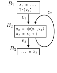
(a)

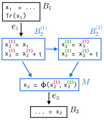
(b)

Figure 5. On the left is a loop which creates an inductive relationship between x${}_{\text{1}}$ and x${}_{\text{2}}$. Partially expanding it as shown on the right allows our data-flow analysis to capture this relationship.

Loop transformation

In the presence of loops, the data-flow rules can fail to capture inductive relationships (e.g., loop-carry dependencies). For example, in Figure LABEL:fig:pita-loop-2, they would be unable to deduce that knowledge of x${}_{\text{1}}$ in $B_{1}$ implies knowledge of x${}_{\text{2}}$ in $B_{3}$. To remedy this, prior to the data-flow analysis, we perform partial loop expansion. This procedure takes a control-flow graph with a loop and transforms it to be acyclic. We accomplish this by duplicating the loop body and removing the back edge. Unlike full loop unrolling, we only keep two cases: the initial case and the inductive case. We note that although this procedure destroys the “correctness” of the program in terms of the values computed, it preserves the relationships (between variables) that are relevant to modeling knowledge. This technique is crucial for analyzing the benchmarks in Section 8. We present more details about the partial loop expansion procedure in Appendix B.

Data-flow initialization and evaluation

Once the program control-flow graph is transformed to account for loops, we proceed to run the data-flow analysis.

We start by initializing data-flow values. We look at all the transmitters in the program. For all $B\in\mathbb{B}$, and for every $e^{\prime}\in E_{\textup{out}}(B)$, we initialize ${{\widehat{K}_{\mathbb{E}}}(e^{\prime})}$ to be the set of all variables in $B$ that are directly passed to a transmitter. This is a direct application of Theorem 2. We also utilize some inter-procedural initialization, but with a unidrectional flow of information. Suppose we are analyzing a program function f that makes a call to some other function $\text{g}_{\text{}}$(x) in block $B$. If previous analysis of g had concluded that the frontier of x within g was the entry block of g, then in our analysis of f we may add $x$ to ${{\widehat{K}_{\mathbb{E}}}(e)}$ for all $e\in E_{\textup{out}}(B)$. This step relies on g having been analyzed prior to f, which is why we must perform our analysis in the order of callees then callers as mentioned before.

We then apply Theorems 3-8 iteratively until we have achieved convergence; that is, until the size of ${\widehat{K}_{\mathbb{E}}}$ has reached a fixed point. Recall that the range of of our data-flow values is $2^{\mathbb{V}}$, which is a powerset lattice of finite height. Our data-flow rules never decrease the size of the data-flow value, i.e. the values can never move down the lattice. Thus, there is a limit to how much the data-flow values can grow before stagnating. This guarantees that our analysis will converge in finite time.

7.2. The Symbolic Execution Pass

We apply the symbolic execution pass on functions that are not fully declassified; our goal is to deduce additional attacker knowledge as detailed in Section 6.2. To that end, we invoke Klee (klee, ) to answer Question 1 with respect to a region $R$ and variable $x$. We are interested in analyzing regions that encompass all transmitters. Let $\textsc{Tx}(\mathbb{B})$ be the set of all blocks which contain at least one transmitter. Any region $R$ such that $\textsc{Tx}(\mathbb{B})\subseteq R$ is a candidate region for the symbolic execution pass. We can find these automatically by looking at all $B\in\mathbb{B}$ and keeping the ones that collectively dominate every transmitter. Then, the regions defined by each of these is a candidate region. Furthermore, any variable which is known in a block that contains a transmitter (even if that variable is itself not transmitted in that block) is a candidate variable. That is, the set of all candidate variables is $\bigcup{{\widehat{K}}_{\mathbb{B}}}\quantity({B^{\prime}})$ for all $B^{\prime}\in\textsc{Tx}(\mathbb{B})$.

We need to run Klee separately for every pair of candidate region and candidate variable. Thus, without loss of generality, we assume for the remainder of this discussion that $R$ is the candidate region and $x$ is the candidate variable. By definition, there is a unique block in $R$, which we’ll denote as $B_{R}$, that dominates all other blocks $R$.

Suppose we are analyzing a program function f. For ease of instrumenting the analysis (below), we assume it has a single terminating block. If it does not, we modify the function such that it does by creating a new terminating block and redirecting all previous ones to it. To run Klee, we write a wrapper which serves as main() and calls f with symbolic arguments. Klee provides an interface for specifying constraints on the values arguments can take. Setting these constraints correctly is important. For example, if b in f(int* a, int b) denotes the length of an array pointed to by a, one should constrain b to be non-negative. Automating deriving argument semantics for this step would be useful, but we consider it out of scope for this paper.

“Asking” Klee if the answer to Question 1 is “yes” or “no” is done by using an assert($\dots$) statement. The assertion is that the answer to Question 1 is “no”: the paths upon which $x$ is not transmitted (if any) are not realizable. To accomplish this, we instrument the program with flags. Let L denote the flag variable. For simplicity, assume L is not SSA, i.e., can be assigned more than once. We add the initialization L$\;=\;$0 in the entry block of the function f. We add the assignment L$\;=\;$-1 in $B_{R}$. In every $B^{\prime}\in\textsc{Tx}(\mathbb{B})$, we add the assignment L$\;=\;$1. In the unique terminating block of the function, we add assert(L$\;\neq\;$-1). If Klee manages to find a counterexample to this assumption, then there is some path through $R$ such that $x$ is not transmitted. Thus, the answer to Question 1 is “yes”. On the other hand, if Klee deduces that the assertion is provably true, then every realizable trace either circumvents the region $R$, or enters it and necessarily transmits $x$, rendering it known. Thus, $x$ is known throughout $R$.

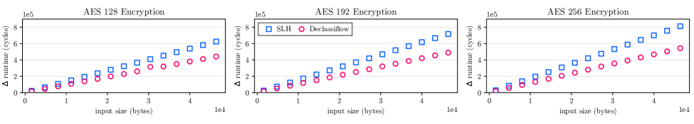
Figure 6. The results of running AES encryption with three different key sizes on inputs of various lengths. We show the raw difference between the runtime (in cycles) of the functions compiled with SLH and the runtime of the baseline (insecure) code. We show the same difference for the Declassiflow protected versions of the functions, i.e., after our analysis is applied. The overhead reduction from the SLH-enabled code to our protected code grows with the size of the input.

7.3. The Protection Pass

We enforce Property 1 with speculation barriers, which we denote as SPEC_BARR. These barriers delay the execution of younger instructions until they are non-speculative. SPEC_BARR conceptually implements protect(*); it indiscriminately applies protection for every variable. That means if the knowledge frontiers for two variables $x$ and $y$ both include some block $B$, only one SPEC_BARR needs to be added to $B$ to enforce the frontier for both $x$ and $y$. Since SPEC_BARR itself is relatively heavyweight, our main tactic to get speedup will be to determine that frontiers (and therefore SPEC_BARR placement) fall outside of critical loops. In that case, for sufficiently long loops, the cost of the SPEC_BARR will be amortized.

We now describe the procedure for placing SPEC_BARR for a program function f. We first clone f to produce $\text{f}^{\prime}$. The latter is what we refer to as the protected version of f. Without loss of generality, suppose that f (and thus $\text{f}^{\prime}$) only makes calls to one other function $\text{g}_{\text{}}$(x) which leaks its argument. Assume a protected version of g exists, denoted $\text{g}_{\text{}}^{\prime}$(x).

We now describe the procedure to protect the internals of $\text{f}^{\prime}$. We compute the joint frontier of locally transmitted variables, i.e. $F_{\text{local}}=\bigcup\mathcal{F}(v)$ for all v in f.

We next need to get the joint frontier of all variables that are not necessarily locally transmitted, but are transmitted by calls to other functions; we denote these as $F_{\text{func}}$. In this example, this would be from calls to g. We can replace calls to $\text{g}_{\text{}}$(x) with calls to $\text{g}_{\text{}}^{\prime}$(x).

The manner in which we enforce protection of $\text{g}^{\prime}$ depends on whether it is a pseudo transmitter or not. Suppose it is a pseudo transmitter and thus can be caller enforced. For purposes of disambiguation, let x${}_{\text{i}}$ denote the argument to the $i$-th call site of $\text{g}_{\text{}}^{\prime}$(x). We need to enforce the union of the frontiers for the leaked x${}_{\text{i}}$. We compute $F_{\text{func}}=\bigcup\mathcal{F}(x_{i})$. If $\text{g}^{\prime}$ is not a pseudo transmitter, it will be callee enforced, and so it will be internally protected, and we would have $F_{\text{func}}=\varnothing$.

We now place SPEC_BARR’s in $\text{f}^{\prime}$. If $\text{f}^{\prime}$ itself is not a pseudo transmitter, then it must be callee enforced. In this case, a SPEC_BARR is placed in every block in $F_{\text{local}}\cup F_{\text{func}}$. However, if $\text{f}^{\prime}$ is a pseudo transmitter, and thus can be caller enforced, then a SPEC_BARR needs to placed in all those same blocks except the entry block of the function. Note, if $\text{f}^{\prime}$ is a pseudo transmitter, then $F_{\text{local}}\cup F_{\text{func}}$ is precisely the entry block of $\text{f}^{\prime}$. As a result, no SPEC_BARR’s will be placed in $\text{f}^{\prime}$. This leads to a useful optimization: if we have a chain of nested calls of pseudo transmitters, we need only a single SPEC_BARR at the top level to protect the full call chain.

This unidirectional inter-procedural strategy is a fairly greedy method for minimizing the total number of SPEC_BARR’s in the program. Taking a global view of the relationship between functions will undoubtedly lead to better barrier placement strategies. However, estimating the cost of barriers will most likely rely on heuristics, and so we leave such a problem to future work.

8. Evaluation

We implement our analysis as an LLVM pass that interoperates with KLEE. We will now evaluate the analysis’ effectiveness in terms of how it can efficiently protect constant-time workloads.

Workloads

We evaluate 3 constant-time workloads: The AES block-cipher encryption from the ctaes repository under the Bitcoin Code organization found on Github (ct-aes, ). The Djbsort constant-time integer sorting algorithm (djbsort, ; djbsort-paper, ). The ChaCha20 stream cipher encryption from the BearSSL library (bearssl_chacha20, ). For each, we applied Declassiflow as described in Sections 6 and 7.

Baselines

We compare against each benchmark unmodified and also to each benchmark compiled with Speculative Load Hardening (SLH) (slh, ). SLH is a Spectre mitigation deployed by LLVM that works by accumulating branch predicate state and using that state to prevent certain instructions from executing speculatively and/or to prevent certain data from being forwarded speculatively. The academic community has shown how SLH, when configured to delay the speculative execution of all transmitters, is sufficient to protect non-speculatively accessed data (SSLH, ; USLH, ). We compare to a weaker variant, called “address SLH” or aSLH. aSLH was designed to protect speculatively-accessed data. It does this by delaying the execution of speculative loads, that have addresses only known at runtime, until they are non-speculative. That is, it considers loads to be instructions that access (return) sensitive data. Since loads are also transmitters, aSLH can be viewed as implementing a subset of the mechanisms required to protect non-speculatively accessed data. Thus, the security provided by Declassiflow is stronger than aSLH and aSLH’s overhead will underestimate the true overhead of SLH in our setting.

All workloads compiled using Declassiflow maintain the branch predicate state (but do not use it to delay instructions/data-flows) needed to support SLH. We do this to provide a conservative overhead estimate: SLH requires this information be maintained across function calls, thus the benchmarks we protect with Declassiflow can interoperate with SLH implemented in a calling context, if needed.

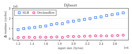
Figure 7. The results of running Djbsort on inputs of various lengths. The y-axis follows the same convention as in Figure 6.

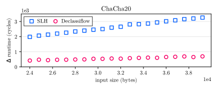
Figure 8. The results of running ChaCha20 on inputs of various lengths. The y-axis follows the same convention as in Figure 6.

Environment setup

We run our experiments on an x86-64 Intel Xeon Gold 6148 machine with Ubuntu 20.04, kernel version 5.4.0-146-generic. We compiled our benchmarks with -O3 and ensured that all versions of the binary differ only in their protection mechanisms. The AES source files were compiled with LLVM version 16 while the Djbsort and ChaCha20 source files were compiled with LLVM version 11. We run Klee in a Docker container based on their official image.

Analysis procedure

To produce protected code, we run the 3 phases of our analysis: The data-flow analysis is run to determine ${\widehat{K}_{\mathbb{E}}}$. Klee is used to compute additions to ${\widehat{K}_{\mathbb{E}}}$. The protection pass is run, which adds barriers. If Klee is not needed to improve the precision of the result of phase , phase may be skipped. For the benchmarks which do go through phase , we provide a static buffer of fixed size that contains symbolic values. We also provide a symbolic value that represents the buffer’s dynamic length. We constrain this symbolic value to be as low as 0 and as high as the length of the static buffer. This static buffer coupled with the length represent the user input to the functions.

Benchmarking methodology

For constant-time AES encryption, we benchmark the top-level functions AES128_encrypt,
AES192_encrypt, and AES256_encrypt, which use key sizes of 128, 192, and 256 bits respectively. We benchmark each of these with inputs of various sizes. The Djbsort and ChaCha20 benchmarks only have one function each that performs the core workload. Thus, we benchmark those two functions, again with inputs of various sizes. Before every call to the function under test, we perform a small series of floating point computations which get their input from disparate locations in memory. The function under test is then only executed if the result is non-zero. This is meant to introduce a branch that is always taken and will be easily predicted as such. The induced speculation is meant to test the effects of the SPEC_BARR’s we place. We use rdtscp to measure timing. To amortize timer function overhead, we time the function calls in groups of 8 and then normalize the result. This batch-of-8 timing represents one “trial”. For every data point, we run 800 trials and discard the first 100 to remove warmup effects of the cache and TLB. We then report the median of the 700 remaining trials.

8.1. Main Result

The full experimental results are presented in Figures 6, 7, and 8. We show the raw difference between the SLH and the Declassiflow versions of the functions with respect to the baseline. The geometric means of the relative overheads of SLH for the encryption functions are 16%, 16%, and 17% for each key size respectively. Meanwhile, the geometric means of the relative overheads of the Declassiflow versions of the functions are 12%, 12%, and 11% respectively. For the Djbsort benchmark, the geometric mean of the relative overhead of SLH is 24%, while the geometric mean of the relative overhead of the Declassiflow version is 3%. For the ChaCha20 benchmark, the geometric mean of the relative overhead of SLH is 7%, while the geometric mean of the relative overhead of the Declassiflow version is 1%.

All three benchmarks make heavy use of loops. Thus, the overhead of SLH increases with the size of the input because the SLH instrumentation is repeatedly encountered. Our analysis tries to prove that the knowledge frontier is outside of the inner loops (ideally, outside of all loops), hence decreasing the frequency that protection mechanisms are encountered. With AES, our analysis discovers that the frontier is outside of just the innermost loops. Thus, while the overhead of the Declassiflow versions grow with input size, they grow slower than that of the SLH-protected version. With Djbsort and ChaCha20, our analysis discovers the frontier is completely outside the main loop. Thus, the overhead of the Declassiflow versions are low and constant. In the Declassiflow version of each of the three benchmarks, only a single SPEC_BARR is statically inserted; though for AES the barrier is placed inside a loop, so it is encountered multiple times dynamically.

Analysis runtime

We now provide details on our analysis’ runtime. Before we start, note that our analysis is not part of the typical code-compile-debug workflow programmers use during development. Instead, we expect it to be run a few times (e.g., once) as a post-processing step to add security on top of otherwise production-ready code. Thus, these overheads may amortize in practice.

The runtimes of all phases except are given in Table 1. The runtime of phase (running Klee) is over two orders of magnitude higher than the runtimes of the other phases, making it the bottleneck. Table 1 also shows how the execution time of Klee scales with respect to the complexity of the program. In this experiment, we vary the length of the static buffer mentioned previously, and along with it the constraints on the symbolic length. This essentially changes the upper bound on the size of the arrays that Klee needs to reason about.

To understand better why Klee runtime scales with buffer size, we now report how buffer size impacts Klee’s execution time. Recall from Sections 6.2 and 7.2 that we need to invoke Klee for every candidate region $R$ and candidate variable $x$ for which we want to answer Question 1. For Djbsort, there are 72 possible candidate variables and 4 candidate regions; thus, we need $72\times 4=288$ invocations of Klee. For ChaCha20, there are 91 candidate variables and 3 candidate regions; thus we need $91\times 3=273$ invocations of Klee. For both benchmarks, we found that the number of invocations does not vary with static buffer size. Each invocation evaluates Klee expressions, which generate what Klee calls “query constructs.” For a given static buffer size, the number of query constructs generated is the same across all invocations. That said, the number of query constructs per invocation increases with the static buffer size. This is predictive of overhead; Figure 9 shows how the time taken for an individual invocation scales closely with the number of query constructs generated.

	DFA	Symbolic Execution				Protection
		$N=4$	$N=8$	$N=16$	$N=32$
AES	1s	–	–	–	–	$<\,$1s
Djbsort	35s	37m	48m	92m	266m	$<\,$1s
ChaCha20	3s	35m	38m	44m	57m	$<\,$1s

Table 1. The runtime of the data-flow analysis (DFA) phase; the protection phase; the symbolic execution phase (end-to-end runtime for various sizes for the symbolic input buffer). Since AES doesn’t use Klee, the data is omitted. Note the difference in units in the Klee column versus the DFA and relaxation column. The numbers are the average of 5 runs rounded to the nearest unit.

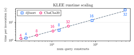
Figure 9. The time taken per invocation vs. the number of query constructs per invocation. Note, for any particular symbolic buffer size, every invocation of Klee will have the same number of query constructs. We plot the median of the time measurements of those invocations. The size of the symbolic buffer associated with any particular datapoint (chosen to match Table 1) is indicated next to it. Note that in Table 1, we are reporting the end-to-end runtime (sum of) for all invocations.

We spend the remainder of Section 8 looking at some of the interesting aspects of each benchmark and explaining how the analysis responds to those aspects.

8.2. AES Encryption

⬇ encrypt(y${}_{\text{1}}$) {  x  =  ...  f(x,y${}_{\text{1}}$)  for (...) { y${}_{\text{2}}$  =  (y${}_{\text{1}}$,y${}_{\text{3}}$) g(x,y${}_{\text{2}}$) y${}_{\text{3}}$  =  y${}_{\text{2}}$  +  1  }  h(x,y${}_{\text{3}}$) }

(a) Original

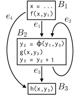
(b) CFG

⬇ encrypt(y${}_{\text{1}}$) {  SPEC_BARR  x  =  ...  $\color[rgb]{0.96875,0,0.40234375}\text{f}^{\prime}$(x,y${}_{\text{1}}$)  for (...) { y${}_{\text{2}}$  =  (y${}_{\text{1}}$,y${}_{\text{3}}$) $\color[rgb]{0.96875,0,0.40234375}\text{g}^{\prime}$(x,y${}_{\text{2}}$) y${}_{\text{3}}$  =  y${}_{\text{2}}$  +  1  }  $\color[rgb]{0.96875,0,0.40234375}\text{h}^{\prime}$(x,y${}_{\text{3}}$) }

(c) Declassiflow

Figure 10. Application of our analysis to AES_encrypt. Functions f, g, and h are pseudo transmitters that leak both their arguments. $\texttt{f}^{\prime}$, $\texttt{g}^{\prime}$ and $\texttt{h}^{\prime}$ are their Declassiflow protected counterparts. NOTE: The figure depicts a highly simplified version of the function that still captures the salient details for our analysis. See Table 2 for the details on the size of the benchmark.

The functions AES128_encrypt, AES192_encrypt, and
AES256_encrypt are each given a plaintext input which can be composed of any number of data blocks. Each function will call AES_encrypt internally for every provided block to encrypt it. AES_encrypt itself will run a specified number of rounds of encryption on the provided block. The various steps of a round of AES encryption are encapsulated in their own functions, which are called by AES_encrypt.

The analysis’ treatment of the function AES_encrypt is an interesting case study since it can be fully protected without the need for symbolic execution. Furthermore, it highlights the importance of our inter-procedural rules. An analogous and highly simplified form of the function (that still captures the salient details for our analysis) and its control-flow graph are depicted in Figures 10a and 10b, respectively. (See Table 2 for the details on the size of the benchmark.) In the figure, f, g, and h represent encapsulations of various operations performed by AES encryption (e.g. mixing columns or adding in the round key). We point out that the variables x and y${}_{\text{1}}$ do not correspond to secret data in the original code; their contents are the addresses of buffers.

Prior to analyzing AES_encrypt, f, g, and h will have already been analyzed and deduced to be pseudo transmitters that leak both of their arguments. From this, the data-flow analysis will be able to conclude that the frontier for every variable is $B_{1}$. The partial loop expansion mentioned in Section 7.1 is crucial to this deduction. Now AES_encrypt will be protected. There are no local transmitters to protect. The calls to f, g, and h can be replaced with their protected counterparts, $\text{f}^{\prime}$missing, $\text{g}^{\prime}$missing, and $\text{h}^{\prime}$missing. Being pseudo transmitters, they need to be caller enforced, and so a SPEC_BARR is placed in $B_{1}$, the frontier of their collective arguments. The Declassiflow protected version of the code is shown in Figure 10c. Since x is leaked internally and cannot be deduced from the argument y${}_{\text{1}}$, AES_encrypt is not a pseudo transmitter and thus cannot be caller enforced.

The crucial difference between the SLH and Declassiflow-protected versions of AES_encrypt is that under SLH, the protection of all the variables is present inside the loop. Since every loop iteration contains a branch that can be speculated, the hardening performed by SLH causes repeated delays. Thus, in the graph we see that the overhead of SLH increases as the size of the input increases. On the other hand, our protected version of AES_encrypt has a single SPEC_BARR, and within the loop body, we call $\text{g}^{\prime}$missing and $\text{h}^{\prime}$missing which do not have hardened loads. Thus, we pay the SPEC_BARR penalty once, but SLH pays a penalty for every load over and over again. This is why our protected function performs much better than its SLH counterpart.

We note that the higher-level functions which we benchmark call the protected version of AES_encrypt (Figure 10c) in a loop. Since AES_encrypt is callee enforced, the number of times the SPEC_BARR is encountered is linear with respect to the size of the input. That is why we see the overhead of the protected function increase with the size of the input as opposed to remaining fixed.

8.3. Djbsort

This benchmark is an interesting case study due to its heavy use of nested loops. The function takes two parameters, an array of integers x and the length of the array N. All transmitters in Djbsort arise from accessing x at various offsets. The core concept of the function is depicted in a highly simplified form (that still captures the salient details for our analysis) in Figure 11. (See Table 2 for the details on the size of the benchmark.) Djbsort cannot be declassified using our data-flow analysis alone. The issue is by the semantics of while (and similarly for) loops, when the program is compiled, the control-flow graph will typically include an edge that bypasses the loop body (${\color[rgb]{0.96875,0,0.40234375}e_{3}}$ from the figure). Ideally, the frontier of x is $B_{2}$ since Tr(x+i) in $B_{2}$ is guaranteed to be encountered once the first branch is crossed, and i will be known at every point due to being an inductive variable with a known starting value. However, because the data-flow analysis assumes $e_{3}$ is traversable, the frontier can be lifted no higher than $B_{3}$. This problem is addressed by symbolic execution as described in Section 6.2. It can deduce that there is no possible execution of Djbsort in which the array x is not accessed at least once. After the symbolic execution pass, our analysis will correctly report that the frontier of x should be $B_{2}$.

The conditional if (N < 2) at the top of the function is crucial for the symbolic execution tool to make the aforementioned deduction. Once the symbolic execution engine proceeds past this branch, it is armed with the path constraint $N\geq 2$. This constraint is necessary to deduce that the loop condition is always satisfied initially, and therefore that x is guaranteed to be leaked.

We note that although symbolic execution is needed to effectively relax Djbsort, it is not be able to do it on its own. Crucially, it is not x that is transmitted, but x + i. The data-flow analysis is needed to deduce that i is always known, and it will do so via partial loop expansion. Only then can the instrumentation for the symbolic execution pass treat Tr(x + i) as though it leaks x.

Since x is only guaranteed to be known after it’s non-speculatively confirmed that $N\,\geq\,2$, a SPEC_BARR must be placed after the if (N < 2). After this point in the program, SLH can be disabled for the whole function.

⬇

 

 

if (N < 2) {

return;

}

i = 0

while (i < N) {

$\color[rgb]{0.05078125,0.39453125,1}{\dots}$  = x[i]

i = i + 1

}

 

 

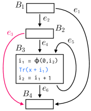
Figure 11. The core of the Djbsort benchmark from the perspective of our analysis. NOTE: The figure depicts a highly simplified version of the function that still captures the salient details for our analysis. See Table 2 for the details on the size of the benchmark.

8.4. ChaCha20

The ChaCha20 benchmark is similar to the Djbsort benchmark in that it involves a series of nested loops and that all transmitters are due to accesses of various arrays. One can intuit from the source code that if the length of the provided input is non-zero, then all arrays’ addresses are guaranteed to be known. Klee must be used to prove this in an attempt to safely remove protections for the entirety of the function. One key difference between ChaCha20 and Djbsort is that in the high-level source code, there is no if statement that short-circuits the function if a zero-length input is provided. However, compilers will often add such checks in the form of a loop “preheader”, and indeed this is what LLVM does for ChaCha20. Thus, from the point of view of our analysis (which is applied to the LLVM IR generated after compilation), the two benchmarks are quite similar in form. We thus omit any discussion of the analysis itself. A single SPEC_BARR is placed after the check for non-zero length but outside any loops, and SLH is disabled for the entire function.

9. Related Work

Prior work Blade (blade, ) and several recent SLH variants (USLH, ; SSLH, ; SpectreDeclassified, ) share Declassiflow’s goal of reducing overhead of speculative execution defenses for constant-time code. Blade protects only speculatively-accessed data: it statically constructs a data-flow graph from mis-speculated loads (which can return secrets) to transmitters and infers a minimal placement of protections that cuts off such data-flow. SSLH (SSLH, ) and USLH (USLH, ) strengthen SLH to protect non-speculatively accessed data. As discussed in Section 8, these schemes will incur a higher performance penalty than Declassiflow while providing comparable security.

selSLH builds on programming language support for public/secret type information (FactLanguage, ), which it uses to selectively apply SLH only on loads into public variables. This approach relies on typed variables, with the type system enforcing that a transmitter’s operand is always typed public. However, this property isn’t preserved on compilation: a machine register rX can hold public and secret values in different program contexts. Therefore, mis-speculation from a context in which rX holds a secret to a context in which rX is public and is an operand to a transmitter can result in rX leaking (deianpldi, , Section 4.2.2). Overall, selSLH, like Blade, doesn’t protect secret non-speculative register data. In contrast, Declassiflow protects both speculatively-accessed data (read from memory under speculation) and secret non-speculative register data, and makes no assumptions on the programming language used.

In Shivakumar et al. (typing-crypto, ), the authors propose language primitives for writing cryptographic code that is protected from Spectre v1. These primitives can be used to implement traditional SLH along with selSLH, and a type system checks that the program meets a provided security definition. Inserting these primitives in code is not automatic and requires developer effort. In theory, their work is compatible with ours as we could use our analysis to relax code protected via their primitives. It could be that more fine-grained (and thus more beneficial) relaxations would be possible.

Finally, several works (InSpectre, ; deianpldi, ; Spectector, ; CSFdef, ) develop static analyses to detect violations of a formal notion of security against speculative leakage, which is based on the idea that a program’s speculative execution should not leak more than its non-speculative execution. Declassiflow also leverages this type of security property, but its goal is to safely relax conservative protections while maintaining security.

10. Conclusion

This paper presented Declassiflow: a static analysis that reduces the amount of protection needed to “take speculative execution off the table” for constant-time programs. The key observation is that as the program’s non-speculative execution makes forward progress, various instructions that reveal their operands over side channels will inevitably execute. Such inevitably-revealed operands need not be protected in the program’s speculative execution. This allows one to safely hoist, consolidate or even remove protection primitives, improving performance.

Longer term, an interesting question will be whether hardware-based schemes such as SPT and software-based schemes such as Declassiflow can be combined to further reduce overhead. These two approaches are complementary, in the sense that a hardware-based scheme can take advantage of fine-grain dynamic information (e.g., the current path taken by the program) while a software-based scheme can take advantage of global knowledge of the control data-flow graph. There are also opportunities to improve Declassiflow as a stand-alone analysis. For example, to automatically deduce protection placement, understand which program paths are realizable, and improve the fidelity in which the analysis understands knowledge (e.g., using ideas from QIF (qif, )).

Acknowledgments

We thank the anonymous reviewers and our (truly superb) shepherd for their valuable feedback. This research was partially funded by NSF grants 1954521, 1942888 and 2154183.

Benchmark	Function	Callees	Num Blocks	Num Edges	Num Instrs
AES	AES128_encrypt	AES_encrypt	4	7	14
	AES_encrypt	LoadBytes, SubBytes, ShiftRows, SaveBytes	3	6	200
	LoadBytes	—	3	5	258
	SubBytes	—	7	10	260
	ShiftRows	—	1	2	177
	SaveBytes	—	3	5	238
Djbsort	int32_sort	—	37	68	205
ChaCha20	br_chacha20_ct	—	12	21	409

Table 2. The size and call structure of each benchmark. In our analysis, we ensure that every block has an input and output edge. For singleton-block functions, we thus add two “dummy edges”, $(\textsc{Entry},B)$ and $(B,\textsc{Exit})$. Notice, Djbsort and ChaCha20 have more complicated control-flow structure than the AES functions, but the AES functions are nested 3 levels deep, requiring our inter-function protection rules.

Appendix A Proofs of Theorems

Theorem 1.

Consider an instruction $I$ of the form Tr(x) in some block $B$ with output edges $e_{o}$. For all $e_{o}$, $x\in{K_{\mathbb{E}}}(e_{o})$.

Proof.

Take any $e_{o}\in E_{\textup{out}}(B)$. Suppose we have a trace $t\in\mathbb{T}$ such that $e_{o}\in t$. By the time $t$ traverses $e_{o}$, it must have already executed Tr(x). By Definition 1, $x$ is known. So by Definition 1, we must have $x\in{K_{\mathbb{E}}}(e_{o})$. ∎

Theorem 2.

Take any edge $e\in\mathbb{E}$. Consider a forward solvable instruction $I$ from anywhere in the control-flow graph, and suppose it is of the form $y=f(x_{1},\dots,x_{N})$. If $x_{i}\in{K_{\mathbb{E}}}(e)$ for all $x_{i}$, then $y\in{K_{\mathbb{E}}}(e)$.

Proof.

Suppose we have a forward solvable instruction of the form $y=f(x_{1},\dots,x_{N})$, and suppose further that on some arbitrary edge $e$ we have $x_{1},\dots,x_{N}\in{K_{\mathbb{E}}}(e)$. By Definition 1, if an execution traverses $e$, then $x_{1},\dots,x_{N}$ are known at that point in time. The attacker can use their knowledge of these variables along with knowledge of $f$ (due to the program being public) to compute $y$. Thus, at that point in time, the attacker knows $y$. By Definition 1, $y\in{K_{\mathbb{E}}}(e)$. ∎

Theorem 3.

Take any edge $e\in\mathbb{E}$. Consider a backward solvable instruction $I$ from anywhere in the control-flow graph, and suppose it is of the form $y=f(x_{1},\dots,x_{N})$. For any $j\in\{{1,\dots,N}\}$, suppose we have all $x_{i\neq j}\in{K_{\mathbb{E}}}(e)$ as well as $y\in{K_{\mathbb{E}}}(e)$. Then $x_{j}\in{K_{\mathbb{E}}}(e)$.

Proof.

Suppose we have a backward solvable instruction of the form $y=f(x_{1},\dots,x_{N})$. Suppose further, without loss of generality, that on some arbitrary edge $e$ we have $y,x_{1},\dots,x_{N-1}\in{K_{\mathbb{E}}}(e)$. By Definition 1, if an execution traverses $e$, then $y,x_{1},\dots,x_{N-1}$ are known at that point in time. The attacker can use their knowledge of these variables along with knowledge of $f$ (due to the program being public) to compute $x_{N}$. Thus, at that point in time, the attacker knows $x_{N}$. By Definition 1, $x_{N}\in{K_{\mathbb{E}}}(e)$. ∎

Theorem 4.

Consider a block $B$. If for some variable $v$ we have $v\in\bigcap{K_{\mathbb{E}}}(e_{i})$ for all realizable $e_{i}$ in $E_{\textup{in}}(B)$, then we have $v\in{K_{\mathbb{E}}}(e_{o})$ for every $e_{o}\in E_{\textup{out}}(B)$.

Proof.

Let $V=\bigcap{K_{\mathbb{E}}}(e_{i})$ for all realizable $e_{i}$ in $E_{\textup{in}}(B)$. Take any $e_{o}\in E_{\textup{out}}(B)$. Now take any $t\in\mathbb{T}$ such that $e_{o}\in t$. There must be some realizable $e^{\prime}\in E_{\textup{in}}(B)$ such that $e^{\prime}\in t$. By construction, for any $v\in V$, we must have $v\in{K_{\mathbb{E}}}({e^{\prime}})$. Note that this is true regardless of what $e^{\prime}$ is. By Definition 1, when $t$ traverses $e^{\prime}$, $v$ is known. By choice of $t$, it then traverses $e_{o}$. At the time $e_{o}$ is traversed, $v$ is known. Thus by Definition 1, $v\in{K_{\mathbb{E}}}(e_{o})$. ∎

Theorem 5.

Consider a block $B$. If for some variable $v$ we have $v\in\bigcap{K_{\mathbb{E}}}(e_{o})$ for all realizable $e_{o}$ in $E_{\textup{out}}(B)$, and if $v$ is not defined in $B$, then we have $v\in{K_{\mathbb{E}}}(e_{i})$ for every realizable $e_{i}\in E_{\textup{in}}(B)$.

Proof.

Let $V=\bigcap{K_{\mathbb{E}}}(e_{o})$ for all realizable $e_{o}$ in $E_{\textup{out}}(B)$. Take any $e_{i}\in E_{\textup{in}}(B)$ and any $t\in\mathbb{T}$ such that $e_{i}\in t$. There must be some realizable $e^{\prime\prime}\in E_{\textup{out}}(B)$ such that $e^{\prime\prime}\in t$. By construction, for any $v\in V$, we must have $v\in{K_{\mathbb{E}}}({e^{\prime\prime}})$. By Definition 1, when $t$ traverses $e^{\prime\prime}$, $v$ is known. By choice of $t$, $e_{i}$ is guaranteed to be traversed. If $v$ is not defined in $B$, then $v$ is guaranteed to be known. Traversing $e_{i}$ guarantees $v$ is known, and so by Definition 1, $v\in{K_{\mathbb{E}}}(e_{i})$. ∎

Theorem 6.

Let $I_{\phi}$ denote a -function of the form $y=\allowbreak\phi(x_{1},\allowbreak\dots,\allowbreak x_{N})$ in block $B$ with $N$ input edges $e_{1},\dots,e_{N}$. The semantics of $I_{\phi}$ are such that $y=x_{i}$ if $e_{i}\in E_{\textup{in}}(B)$ is traversed to reach $B$. If for all realizable $e_{i}$ we have $x_{i}\in{K_{\mathbb{E}}}(e_{i})$, then for every output edge $e^{\prime}$, $y\in{K_{\mathbb{E}}}({e^{\prime}})$.

Proof.

Suppose we have a trace $t\in\mathbb{T}$ such that for some $e^{\prime}\in E_{\textup{out}}(B)$ we have $e^{\prime}\in t$. There must be some edge from $E_{\textup{in}}(B)$ that is also contained in $t$. Without loss of generality, we’ll call this edge $e_{j}$ and suppose $e_{j}\in t$. By assumption, $x_{j}\in{K_{\mathbb{E}}}(e_{j})$. By the semantics of $I_{\phi}$, when traversing $e^{\prime}$, we have $y=x_{j}$. By Theorem 3, $y\in{K_{\mathbb{E}}}(e_{j})$ as well. Since we assumed $e_{j}$ could be any input edge, $y$ is guaranteed to be known so long as $e^{\prime}\in t$. Thus, by Definition 1, $y\in{K_{\mathbb{E}}}({e^{\prime}})$. ∎

Theorem 7.

Let $I_{\phi}$ denote a -function of the form $y=\allowbreak\phi(x_{1},\allowbreak\dots,\allowbreak x_{N})$ in a block $B$ with input edges $e_{1},\dots,e_{N}$. The semantics of $I_{\phi}$ are the same as in Theorem 6. If for all realizable output edges $e^{\prime}$ we have $y\in{K_{\mathbb{E}}}({e^{\prime}})$, then for every $e_{i}$ we have $x_{i}\in{K_{\mathbb{E}}}(e_{i})$.

Proof.

Consider an arbitrary input edge $e_{i}\in E_{\textup{in}}(B)$. Take any output edge $e^{\prime}\in E_{\textup{out}}(B)$ and suppose $y\in{K_{\mathbb{E}}}({e^{\prime}})$. Suppose further we have a trace $t\in\mathbb{T}$ such that $e_{i},e^{\prime}\in t$. By choice of $t$, $y=x_{i}$. We see that when $e_{i}$ is traversed, we are guaranteed to know $y$, and as a result, $x_{i}$. Thus, by Definition 1, $x\in{K_{\mathbb{E}}}(e_{i})$. ∎

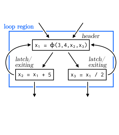
(a) A natural loop.

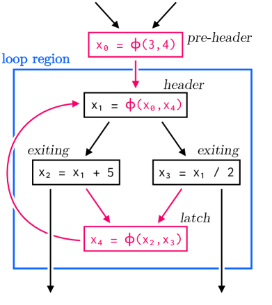
(b) The natural loop, “simplified”.

Figure 12. A natural loop (left) is transformed into a simple loop (right) by creating a pre-header node and merging the two original latch nodes into a single new one. The original inductive- is now a two-way -function. The nodes that were originally exiting blocks remain as such.

Appendix B Partial Loop Expansion

B.1. The Basic Structure of Loops

Generally speaking, a loop is any cycle in the control-flow graph. However, we are primarily concerned with “natural” loops [3]. The natural loop associated with a back edge $(B_{j},B_{i})$ is a set of nodes containing $B_{i}$, $B_{j}$, and all nodes from which there exists a path to $B_{j}$ that does not contain $B_{i}$. The key property of a natural loop is that there is a single node, the header, that dominates all other nodes in the loop. The header node is the destination of the back edge. If two natural loops have different headers, then either the loops are nested or are completely disjoint. It is possible for two natural loops to share a header; it’s standard to treat such a case as a single loop with two back edges.

We adopt terminology used by LLVM [31]. A latch is any node that has a back edge leading to the header of the loop. An exiting node is one that is inside the loop and has an edge leading to a node outside the loop. An exit node is the destination of an exiting node.

We define an inductive- as a -function where at least one of the incoming edges is a back edge. An inductive- selects between two types of values: initial values — the initial versions of a variable that is a constant or another variable from outside the loop; inductive values — the versions of a variable that come from the previous iteration of the loop. An inductive variable is any variable that is the output of an inductive-. Consider the following loop in non-SSA form (left) and SSA form (right),

⬇

x = 1

for (...) {

x++

print(x)

}

⬇

for (...) {

x${}_{\text{1}}$ = (1,x${}_{\text{2}}$missing)

x${}_{\text{2}}$ = x${}_{\text{1}}$ + 1

print(x${}_{\text{2}}$)

}

The inductive- assigns to the inductive variable x${}_{\text{1}}$. It selects the initial value 1 when the loop is first entered and the inductive value x${}_{\text{2}}$ in every iteration after.

A natural loop may have a header with several predecessors and/or multiple latch nodes. LLVM will attempt to transform such loops into what we refer to as a simple loop. The first key property of a simple loop is that the header has only one predecessor, known as the pre-header. The second key property is that there is only one back edge into the header [31]. Figure 12 shows an example of a natural loop transformed into a simple loop.

In a simple loop, the inductive- is always a two-way -function. Furthermore, in the first iteration of the loop, we know the inductive- will collapse into a unique initial value while in every subsequent iteration, the inductive- will collapse into a unique inductive value. When dealing with natural loops in general, things aren’t so easy. For example, in Figure 12a, we know that the inductive- will return either 3 or 4 in the first iteration and either x${}_{\text{2}}$ or x${}_{\text{3}}$ in subsequent iterations, but we can’t conclude anything more than that.

B.2. Loop Expansion Procedure

In a nutshell, partial loop expansion is a transformation which duplicates the loop region. It is a way to compactly model the dynamic definitions of SSA variables that may occur in loops. The general procedure is depicted in Figure 13. Figure 13a is an abstraction of the simple loop from Figure 12b. The substructure within the loop has been condensed into a single “super-node” denoted $\mathbf{Bmissing}$. Figure 13b shows the partial expansion of the loop. There are now two copies of the original super-node, denoted $\mathbf{Bmissing}^{(1)}$ and $\mathbf{Bmissing}^{(2)}$. $\mathbf{Bmissing}^{(1)}$ is identical to $\mathbf{Bmissing}$ except all inductive-’s have been replaced with assignments of the initial values. $\mathbf{Bmissing}^{(2)}$ is identical to $\mathbf{Bmissing}$ except all inductive-’s have been replaced with assignments of the inductive values. Essentially, the path $P\allowbreak{\shortrightarrow}\allowbreak\mathbf{Bmissing}^{(1)}\allowbreak{\shortrightarrow}\allowbreak M\allowbreak{\shortrightarrow}\allowbreak X_{?}$ models the case where a loop is iterated once and the path $P\allowbreak{\shortrightarrow}\allowbreak\mathbf{Bmissing}^{(1)}\allowbreak{\shortrightarrow}\allowbreak\mathbf{Bmissing}^{(2)}\allowbreak{\shortrightarrow}\allowbreak M\allowbreak{\shortrightarrow}\allowbreak X_{?}$ models the case where a loop is iterated at least twice. Any variable $v$ that is defined in $\mathbf{Bmissing}$ is renamed to $v^{(1)}$ in $\mathbf{Bmissing}^{(1)}$ and $v^{(2)}$ in $\mathbf{Bmissing}^{(2)}$. Duplicating the variables like this allows us to model the dynamic definitions of variables. The new multiple definitions of $v$ need to be consolidated before reaching any usage of the original variable $v$ by a block after the loop. We can accomplish this by using a “merge node” $M$ that contains the instruction v = (v${}_{\text{}}^{\text{(1)}}$,v${}_{\text{}}^{\text{(2)}}$).

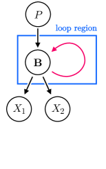
(a) A simple loop.

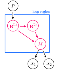
(b) Its partial expansion.

Figure 13. Converting a simple loop into a DAG.

B.3. Example

We’ll look at the loops in Figure 14. They are both identical except in the assignment to x${}_{\text{3}}$. We use <?> to represent an unknown value. We’ll see that these two loops have different implications for knowledge and that partial loop expansion is required to treat them appropriately.

Look at the loop in Figure 14a. If we iterate the loop exactly once, we have that $x_{2}=x_{1}$, and so Tr(x${}_{\text{1}}$) leads to $x_{2}$ being known. However, if we iterate the loop more than once, then $x_{2}$ is actually equal to $x_{3}$, which is unknown. When an execution traverses $e_{3}$, whether $x_{2}$ is known at that point in time depends on the number of times we iterated the loop. By Definition 1, we must have $x_{2}\notin{K_{\mathbb{E}}}(e_{3})$. Now look at Figure 14b. One can see that the values of x${}_{\text{1}}$, x${}_{\text{2}}$, and x${}_{\text{3}}$ are all directly connected and thus equivalent in terms of knowledge; so we ought to have $x_{2}\in{K_{\mathbb{E}}}(e_{3})$. In summary, to achieve both precision and soundness, we need $x_{2}\notin{{\widehat{K}_{\mathbb{E}}}(e_{3})}$ when analyzing the program in Figure 14a and $x_{2}\in{{\widehat{K}_{\mathbb{E}}}(e_{3})}$ when analyzing the program in Figure 14b.

Figure 15 shows the partial expansions of the loops from Figure 14. Looking at the path $B_{1}\allowbreak{\shortrightarrow}\allowbreak B_{2}^{(1)}\allowbreak{\shortrightarrow}\allowbreak M\allowbreak{\shortrightarrow}\allowbreak B_{3}$ in both 15a and 15b, we see there is a direct data-flow from x${}_{\text{1}}$ to x${}_{\text{2}}$ in both loops. Looking at the path $B_{1}\allowbreak{\shortrightarrow}\allowbreak B_{2}^{(1)}\allowbreak{\shortrightarrow}\allowbreak B_{2}^{(2)}\allowbreak{\shortrightarrow}\allowbreak M\allowbreak{\shortrightarrow}\allowbreak B_{3}$, we see there is still a direct data-flow from x${}_{\text{1}}$ to x${}_{\text{2}}$ in 15b. However, there is no such data-flow in 15a due to the assignment of <?> to x${}_{\text{3}}^{\text{(1)}}$. x${}_{\text{2}}^{\text{(2)}}$ represents the dynamic definition of x${}_{\text{2}}$ in the second iteration and beyond. Saying that the data-flow of x${}_{\text{1}}$ doesn’t reach x${}_{\text{2}}^{\text{(2)}}$ is equivalent to saying that after the first iteration, x${}_{\text{1}}$ and x${}_{\text{2}}$ are no longer connected via data-flow. Running the data-flow analysis yields $x_{2}\notin{{\widehat{K}_{\mathbb{E}}}(e_{3})}$ for Figure 14a and $x_{2}\in{{\widehat{K}_{\mathbb{E}}}(e_{3})}$ for Figure 14b.

This procedure is needed to declassify inductive code, e.g. i = 0; while(i < N) {T(i); i++}. This is crucial for declassifying the benchmarks in Section 8.

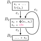
(a) Potential unsoundness.

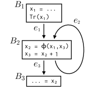
(b) Potential imprecision.

Figure 14. Loops that are problematic for the data-flow analysis unless we use partial loop expansion. See Figure 15.

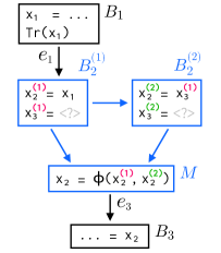
(a) Partial expansion of Figure 14a.

(b) Partial expansion of Figure 14b

Figure 15. The partial expansions of the loops from Figure 14.

References

- [1] ChaCha20 (BearSSL). https://bearssl.org/.
- [2] LLVM Language Reference Manual. https://llvm.org/docs/LangRef.html.
- [3] Alfred V. Aho, Monica S. Lam, Ravi Sethi, and Jeffrey D. Ullman. Compilers: Principles, Techniques, and Tools (2nd Edition). Addison-Wesley Longman Publishing Co., Inc., USA, 2006.
- [4] Marc Andrysco, David Kohlbrenner, Keaton Mowery, Ranjit Jhala, Sorin Lerner, and Hovav Shacham. On subnormal floating point and abnormal timing. In Oakland’15.
- [5] Roberto Baldoni, Emilio Coppa, Daniele Cono D’elia, Camil Demetrescu, and Irene Finocchi. A survey of symbolic execution techniques. In ACM Comput. Surv. May, 2018.
- [6] Enrico Barberis, Pietro Frigo, Marius Muench, Herbert Bos, and Cristiano Giuffrida. Branch history injection: On the effectiveness of hardware mitigations against cross-privilege Spectre-v2 attacks. In Security’22.
- [7] Daniel J. Bernstein. Curve25519: New diffie-hellman speed records. In PKC’06.
- [8] Daniel J. Bernstein. The Poly1305-AES message-authentication code. In FSE’05.
- [9] Daniel J. Bernstein, Chitchanok Chuengsatiansup, Tanja Lange, and Christine van Vredendaal. Ntru prime: Reducing attack surface at low cost. In SAC’17.
- [10] Atri Bhattacharyya, Alexandra Sandulescu, Matthias Neugschwandtner, Alessandro Sorniotti, Babak Falsafi, Mathias Payer, and Anil Kurmus. SMoTherSpectre: Exploiting speculative execution through port contention. In CCS’19.
- [11] Bitcoin Code. ctaes. https://github.com/bitcoin-core/ctaes.
- [12] Tevfik Bultan. Quantifying information leakage using model counting constraint solvers. In VSTTE’20.
- [13] Cristian Cadar, Daniel Dunbar, and Dawson Engler. Klee: Unassisted and automatic generation of high-coverage tests for complex systems programs. In OSDI’08.
- [14] Sunjay Cauligi, Craig Disselkoen, Klaus v. Gleissenthall, Dean Tullsen, Deian Stefan, Tamara Rezk, and Gilles Barthe. Constant-time foundations for the new Spectre era. In PLDI’20.
- [15] Sunjay Cauligi, Gary Soeller, Brian Johannesmeyer, Fraser Brown, Riad S. Wahby, John Renner, Benjamin Grégoire, Gilles Barthe, Ranjit Jhala, and Deian Stefan. FaCT: A DSL for timing-sensitive computation. In PLDI’19.
- [16] Kevin Cheang, Cameron Rasmussen, Sanjit A. Seshia, and Pramod Subramanyan. A Formal Approach to Secure Speculation. In CSF’19.
- [17] Rutvik Choudhary, Jiyong Yu, Christopher W. Fletcher, and Adam Morrison. Speculative Privacy Tracking (SPT): Leaking information from speculative execution without compromising privacy. In MICRO’21.
- [18] Bart Coppens, Ingrid Verbauwhede, Koen De Bosschere, and Bjorn De Sutter. Practical mitigations for timing-based side-channel attacks on modern x86 processors. In Oakland’09.
- [19] R. Cytron, J. Ferrante, B. K. Rosen, M. N. Wegman, and F. K. Zadeck. An efficient method of computing static single assignment form. In POPL’89.
- [20] Daniel J. Bernstein. djbsort. https://sorting.cr.yp.to.
- [21] Jacob Fustos, Farzad Farshchi, and Heechul Yun. Spectreguard: An efficient data-centric defense mechanism against spectre attacks. In DAC’19.
- [22] Google/LLVM. Speculative load hardening. https://llvm.org/docs/SpeculativeLoadHardening.html, Published 2018.
- [23] Johann Großschädl, Elisabeth Oswald, Dan Page, and Michael Tunstall. Side-channel analysis of cryptographic software via early-terminating multiplications. In ICISC’09.
- [24] Roberto Guanciale, Musard Balliu, and Mads Dam. InSpectre: Breaking and fixing microarchitectural vulnerabilities by formal analysis. In CCS’20.
- [25] Marco Guarnieri, Boris Köpf, José F. Morales, Jan Reineke, and Andrés Sánchez. Spectector: Principled detection of speculative information flows. In Oakland’20.
- [26] Marco Guarnieri, Boris Köpf, Jan Reineke, and Pepe Vila. Hardware-software contracts for secure speculation. In Oakland’21.
- [27] Shay Gueron. Efficient software implementations of modular exponentiation. In IACR ePrint’11.
- [28] Paul Kocher, Daniel Genkin, Daniel Gruss, Werner Haas, Mike Hamburg, Moritz Lipp, Stefan Mangard, Thomas Prescher, Michael Schwarz, and Yuval Yarom. Spectre attacks: Exploiting speculative execution. In Oakland’19.
- [29] Paul C. Kocher. Timing attacks on implementations of diffie-hellman, rsa, dss, and other systems. In CRYPTO’96.
- [30] F. Liu, Y. Yarom, Q. Ge, G. Heiser, and R. B. Lee. Last-level cache side-channel attacks are practical. In Oakland’15.
- [31] LLVM Project. Llvm loop terminology (and canonical forms).
- [32] Kevin Loughlin, Ian Neal, Jiacheng Ma, Elisa Tsai, Ofir Weisse, Satish Narayanasamy, and Baris Kasikci. DOLMA: Securing speculation with the principle of transient non-observability. In Security’21.
- [33] Giorgi Maisuradze and Christian Rossow. Ret2spec: Speculative execution using return stack buffers. In CCS’18.
- [34] Ross Mcilroy, Jaroslav Sevcik, Tobias Tebbi, Ben L. Titzer, and Toon Verwaest. Spectre is here to stay: An analysis of side-channels and speculative execution. In ArXiv.
- [35] David Molnar, Matt Piotrowski, David Schultz, and David Wagner. The program counter security model: Automatic detection and removal of control-flow side channel attacks. IACR ePrint’05.
- [36] Marco Patrignani and Marco Guarnieri. Exorcising spectres with secure compilers. In CCS’21.
- [37] Ashay Rane, Calvin Lin, and Mohit Tiwari. Raccoon: Closing digital side-channels through obfuscated execution. In Security’15.
- [38] Basavesh Ammanaghatta Shivakumar, Jack Barnes, Gilles Barthe, Sunjay Cauligi, Chitchanok Chuengsatiansup, Daniel Genkin, Sioli O’Connell, Peter Schwabe, Rui Qi Sim, and Yuval Yarom. Spectre declassified: Reading from the right place at the wrong time. In Oakland’23.
- [39] Basavesh Ammanaghatta Shivakumar, Gilles Barthe, Benjamin Grégoire, Vincent Laporte, Tiago Oliveira, Swarn Priya, Peter Schwabe, and Lucas Tabary-Maujean. Typing high-speed cryptography against spectre v1. In IACR ePrint’22.
- [40] Marco Vassena, Craig Disselkoen, Klaus von Gleissenthall, Sunjay Cauligi, Rami Gökhan Kıcı, Ranjit Jhala, Dean Tullsen, and Deian Stefan. Automatically eliminating speculative leaks from cryptographic code with Blade. In POPL’21.
- [41] Jose Vicarte, Pradyumna Shome, Nandeeka Nayak, Caroline Trippel, Adam Morrison, David Kohlbrenner, and Christopher W. Fletcher. Opening Pandora’s box: A systematic study of new ways microarchitecture can leak private data. In ISCA’21.
- [42] Ofir Weisse, Ian Neal, Kevin Loughlin, Thomas Wenisch, and Baris Kasikci. NDA: Preventing speculative execution attacks at their source. In MICRO’19.
- [43] Johannes Wikner and Kaveh Razavi. RETBLEED: Arbitrary speculative code execution with return instructions. In Security’22.
- [44] Yuval Yarom and Katrina Falkner. Flush+Reload: A high resolution, low noise, L3 cache side-channel attack. In Security’14.
- [45] Jiyong Yu, Lucas Hsiung, Mohamad El Hajj, and Christopher W. Fletcher. Data oblivious ISA extensions for side channel-resistant and high performance computing. In NDSS’19.
- [46] Jiyong Yu, Namrata Mantri, Josep Torrellas, Adam Morrison, and Christopher W. Fletcher. Speculative data-oblivious execution: Mobilizing safe prediction for safe and efficient speculative execution. In ISCA’20.
- [47] Jiyong Yu, Mengjia Yan, Artem Khyzha, Adam Morrison, Josep Torrellas, and Christopher W. Fletcher. Speculative taint tracking (STT): A comprehensive protection for speculatively accessed data. In MICRO’19.
- [48] Zhiyuan Zhang, Gilles Barthe, Chitchanok Chuengsatiansup, Peter Schwabe, and Yuval Yarom. Ultimate SLH: Taking speculative load hardening to the next level. In Security’23.