A Hierarchical Nearest Neighbour Approach to Contextual Bandits
Abstract
In this paper we consider the adversarial contextual bandit problem in metric spaces. The paper “Nearest neighbour with bandit feedback" tackled this problem but when there are many contexts near the decision boundary of the comparator policy it suffers from a high regret. In this paper we eradicate this problem, designing an algorithm in which we can hold out any set of contexts when computing our regret term. Our algorithm builds on that of “Nearest neighbour with bandit feedback" and hence inherits its extreme computational efficiency.
1 Introduction
We consider the contextual bandit problem in metric spaces. In this problem we have some (potentially unknown) metric space of bounded diameter. We assume that we have access to an oracle for computing distances. On each trial we are given a context and must choose an action before observing the loss/reward generated by that action. In this paper the contexts are considered implicit and we define to be the distance between and .
This problem has been well-studied in the stochastic case (see e.g. [11], [10], [9] and references therein). In this paper we consider the fully adversarial problem in which no assumptions are made at all about the metric space, context sequence, or loss sequence. As far as we are aware the first non-trivial result for the fully adversarial problem was given by the recent paper [7] which bounds the regret with respect to any policy. This regret bound is fantastic when the contexts partition into well separated clusters and the policy is constant on each cluster. However, the bound is poor when there exist many contexts lying close to the decision boundary of the policy. In order to (partially) rectify this [7] proposed using binning as a preprocessing step. We note that the optimal bin radius can be implicitly learnt via a type of doubling trick, although this was not discussed in [7]. The problem with this is that for different parts of the metric space the optimal bin radii will be different. But [7] can only learn a constant bin radius - leading to poor performance. In this paper we fully rectify this problem, designing a new (but related) algorithm HNN in which, in the loss bound, we can hold out any set of contexts (which we call a margin - i.e. points near the decision boundary) when computing the regret term. In Section 2 we give an example of how we improve over [7]. We note, however, that in cases where the contexts partition into well separated clusters and the policy is constant on each cluster it may be advantageous to use simple nearest neighbour as in [7].
To achieve this improvement we will utilise the meta-algorithm CBNN of [7] which receives, on each trial , only some (we note that in [7] the notation was used instead). [7] analysed the case for when is chosen such that is an approximate nearest neighbour of in the set . In this paper we use a different choice of which we call an approximate hierarchical nearest neighbour. In approximate hierarchical nearest neighbour we will construct, online, a partition of of the trials seen so far into different levels. On each trial the algorithm then uses approximate nearest neighbour on each level. will then be chosen, in a specific way, from one of these approximate nearest neighbours. We note that since our algorithm HNN is based on CBNN it inherits its extreme computational efficiency - having a per trial time complexity polylogarithmic in both the number of trials and number of actions when our dataset has an aspect ratio polynomial in the number of trials (which can be enforced by binning) and our metric space has bounded doubling dimension.
We note that, when using exact nearest neighbour, the process of inserting a given trial into our data-structure is essentially the same as the process of constructing a new bin in [11]. However, the objectives of the data-structures are very different and they are analysed in very different ways (our analysis being far more involved than that of [11]). Nevertheless, we cite [11] as an inspiration for this paper.
2 The Issue with Nearest Neighbour
We now give an example of the issue with the algorithm (using binning with nearest neighbour) proposed by [7]. We will call this algorithm (when implicitly learning the optimal bin radius via a form of doubling trick) NN. For simplicity let’s assume that the parameter , of NN and HNN, is set equal to a constant, although the argument easily extends to tuned parameter values as well. Consider two disjoint balls in with radii equal to and respectively. Assume that each ball has contexts distributed uniformly over it. Suppose we have two actions and a comparator policy such that the decision boundary (of the policy) on each ball is a straight line going through the ball’s centre. This is depicted in Figure 1.
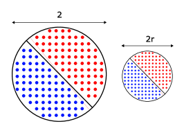
First let’s analyse NN when working on each ball as a seperate problem. Given a binning radius of , the regret of NN on is and the regret of NN on is . For both these problems the optimal value of leads to a regret of .
However, things change when NN is working on both balls at the same time. In this case, given a binning radius of , the regret of NN is:
i.e. the sum of the regrets on both balls. This means that the optimal value of leads to a regret of which can be dramatically higher than if the balls were learnt separately. In fact, when this bound is vacuous - meaning that binning is not helping at all. Our algorithm HNN, however, has a regret of whenever is polynomial in - the same as if the balls were learnt seperately.
When working in for , the improvement of HNN over NN is even stronger. To see this note that the regret of NN when working on both balls is:
so that the optimal value of gives us a regret of which becomes vacuous at . HNN, on the other hand, achieves a regret of whenever is polynomial in - the same as if the balls were learnt seperately.
3 Problem Description
We consider the following game between Nature and Learner. We have trials and actions. Nature first chooses a matrix satisfying the following conditions:
-
•
For all we have .
-
•
For all we have .
-
•
For all we have . For simplicity we will assume, without loss of generality, that for all with we have . This is without loss of generality since if then the trials and are equivalent. Dealing with equivalent trials is straightforward in the CBNN algorithm of [7] upon which our algorithm HNN is based. Trials equivalent to any proceeding trials will be ignored in the data-structure that we construct so have no effect on the computational complexity.
-
•
For all we have . This property is called the triangle inequality.
We note that is a metric over . Intuitively, every trial is implicitly associated with a context and for all we have that is a measure of how similar is to (a smaller value of means a greater similarity). For all trials and actions Nature chooses a probability distribution over and a loss is then drawn from . We note that Learner has knowledge of only and (although the requirement of knowledge of can be removed by a simple doubling trick). The game then proceeds in trials. On trial the following happens:
-
1.
For all Nature reveals to Learner.
-
2.
Learner chooses an action .
-
3.
Nature reveals the loss to Learner.
The aim of Learner is to minimise the cumulative loss:
Note that, since Nature has complete control over each distribution , our problem generalises the fully adversarial problem (which is the special case in which each distribution is a delta function). We are considering this generalised problem in order for our bound to be better when there is an element of stochasticity in Nature’s choices.
4 The Algorithm
We now describe our algorithm HNN. The algorithm takes parameters and . We define . Given a non-empty set and a trial , a -nearest neighbour of in the set is any trial in which:
We utilise the algorithm CBNN [7] with parameter as a subroutine. During the algorithm we will associate each trial with a number and initialise by setting . On each trial we do the following:
-
1.
-
2.
For all set
-
3.
For all let be a -nearest neighbour of in
-
4.
Let be the maximum value of such that
-
5.
-
6.
-
7.
Input into CBNN
-
8.
Select equal to the output of CBNN
-
9.
Receive
-
10.
Update CBNN with
We note that when we can maintain, for each , a navigating net [5] over the set in order to rapidly find .
5 Performance
We now bound the expected cumulative loss of HNN. We first define the various constants used in this section. Let be any value in . We note that the algorithm has no knowledge of . We define:
We define the aspect ratio of our dataset as:
A policy is any vector . A margin is any subset . Suppose we have a policy and a margin such that there exists with . Note that the algorithm has no knowledge of either or . For all we define:
We define:
and define as the maximum cardinality of any set in which for all with we have:
For all define:
and define:
noting that for all we have so that . HNN achieves the following performance:
Theorem 5.1.
The expected cumulative loss of HNN is bounded by:
The running time of HNN is in and, when and has bounded doubling dimension, is also in . HNN requires only space.
We now point out the effect of the choice of the margin on our bound. Note that increasing increases and (for some trials ). The increase in (for some ) can decrease the value which helps us. However, the increase in (for some ) can cause to grow - potentially increasing which hurts us. Hence, there will be a sweet-spot - the optimal margin . Trials in the optimal margin will correspond to contexts that are close to the decision boundary of the policy (but just how close will depend on the location of the context and the density of contexts in its vicinity).
We note that we can use binning to enforce that is polynomial in - hence ensuring polylogarithmic time per trial when has bounded doubling dimension and . To do this we choose some with polynomial in and, on any trial such that there exists with we treat as equivalent to (in CBNN) and ignore in our data-structure. We note, however, that this process can have an effect on the loss bound.
6 When in Euclidean Space
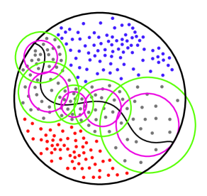
In order to give insight into Theorem 5.1 we now analyse it in the case that the (implicit) contexts lie in the euclidean space (for some constant ) and our metric is the euclidean metric, giving a relatively simple loss bound. We note, however, that we do not use the full power of Theorem 5.1 here - for instance, we crudely bound by when .
We make the following definitions. For all let be the euclidean norm of . Given and we define the ball:
Here we assume that there exists a sequence of contexts such that for all we have . An extended policy is any function . Consider any such extended policy . We define the decision boundary as:
Theorem 5.1 then gives us the following.
Theorem 6.1.
Choose any constants and . Suppose we have some and any sequence with:
-
•
-
•
We define to be the set of all in which there exists with . The expected cumulative loss of HNN (with any constant ) is then bounded by:
In Figure 2 we give an example of the objects appearing in Theorem 6.1.
7 Proof of Theorem 5.1
We now prove Theorem 5.1. We will often use the fact that, for all , we have and in this analysis.
Definition 7.1.
Consider the rooted tree with vertex set such that, for all , we have that is the parent of . Let be the set of leaves of this tree. Given we then define to be the set of all descendants of and define to be the set of all ancestors of .
Lemma 7.2.
For all with and we have that .
Proof.
Suppose, for contradiction, the converse: that . Without loss of generality assume . Let and for all let be as created by the algorithm on trial . Let . Since is a -nearest neighbour of in the set (which contains ) we must have that . But from the algorithm we have that is the maximum value of such that so since we have a contradiction. ∎
Definition 7.3.
Define to be the set of all trials in which for all with and we have .
Lemma 7.4.
Given with and we have .
Proof.
Noting that we fix and prove by induction on . When we have so the result is immediate. Now suppose, for some , that the inductive hypothesis holds for all with . Now take with . Since and we have . So since we have, by the inductive hypothesis, that . Now take any with and . From the algorithm we have that and hence, by the triangle inequality, we have:
Similarly we have . So since and we must have that . Hence, we must have that so the result holds by induction. ∎
Definition 7.5.
Let be the set of all such that either:
-
•
and
-
•
and
Definition 7.6.
Let be the set of all such that there does not exist with and
Definition 7.7.
For any let be equal to the set of all in which
Lemma 7.8.
Given and we either have that there exists with or that there exists some with and
Proof.
If there exists with then we’re done so assume otherwise. We prove by induction on . We immediately have the result for by choosing . Now suppose, for some , that the inductive hypothesis holds when and consider the case that . By the inductive hypothesis choose with and . Since we have, by definition of , that there exists with and . By the triangle inequality we then have:
If it was the case that we would have, from this inequality, that which is a contradiction. Hence, we have . Since and we have . By the above inequality we then have the result by choosing . This completes the inductive proof. ∎
Lemma 7.9.
Given there exists with .
Proof.
Suppose, for contradiction, the converse. By Lemma 7.8 we then have, for all , that there exists some with . By choosing we then have that there exists with which is impossible. ∎
Lemma 7.10.
For all and we have .
Proof.
Suppose, for contradiction, that there exists and with . Then by definition of we have and . Since we then have:
So since we have which, since and , contradicts the fact that . ∎
Lemma 7.11.
For all we have .
Proof.
Lemma 7.12.
For all we have
Proof.
By definition of we immediately have that either or . By Lemma 7.4 we then have that . Hence, by definition of and since , we can choose with and and . Since we can, without loss of generality, assume that which means, since , that . By the triangle inequality and the fact that we then have:
Rearranging then gives us the desired result. ∎
Lemma 7.13.
For all with we have .
Proof.
Lemma 7.14.
We have
Proof.
Immediate from Lemma 7.13 and the definition of . ∎
Lemma 7.15.
For all we have
Proof.
Lemma 7.16.
We have
Proof.
Lemma 7.17.
Suppose we have some such that for all we have . Then .
Proof.
We prove by induction on . If then we have so that we immediately have (since there exists with ). Given some suppose that the inductive hypothesis holds for all with . Now consider any with . Note that for all we have so that . Since we then have, by the inductive hypothesis, that . If it was the case that we would then have, by definition of , that . But since this would be a contradiction. Hence, . This completes the inductive proof. ∎
Lemma 7.18.
For all there exists an such that .
Proof.
Assume, for contradiction, the converse: that there exists no with . This means that for all we have . So choose some . Since we have, for all , that . By Lemma 7.17 we hence have that . But since this would mean that which, since , is a contradiction. ∎
Definition 7.19.
Define the policy inductively from to such that:
-
•
If and there does not exist some with then (or is arbitrary when ).
-
•
If and there exists some with then choose such that there exists with and . Note that by definition of such an does indeed exist (but is not unique - we choose any valid ).
-
•
If and there does not exist with , we have . Since this is defined.
-
•
If and there exists with then . Note that by definition of we have that is uniquely defined.
Lemma 7.20.
Given with there exists with .
Proof.
By Lemma 7.18 choose such that . Assume, for contradiction, that . Then we must have . This means that and hence, by definition of , we have that . So since we have both and we have, by Lemma 7.4, that both and . Since we must then have, by definition of , that there exists with . Since we have, by the triangle inequality, that:
so since and we have, by definition of and since , that . We also have, by definition of and since both and , that . But this means that which is a contradiction. We have hence shown that . ∎
Lemma 7.21.
Given with we have that or that there exists such that .
Proof.
Assume, for contradiction, that and there does not exist such that . By Lemma 7.20 we have that there exists with . Since we have so since we have . If then, by definition of , we have and if we have, again by definition of , that . In either case there exists with . By Lemma 7.4 this means that . So since we have, from definition of , that there exists some with . But since this would imply that which is a contradiction. ∎
Definition 7.22.
Let be the set of all such that and .
Lemma 7.23.
For all there exists such that .
Proof.
Lemma 7.24.
We have
Proof.
Lemma 7.25.
For all with we have
Proof.
We hold fixed and prove by reverse induction on (i.e. from to ). When we have and hence so the result holds trivially. Now suppose, for some , it holds when . We now show that it holds when which will complete the inductive proof. So take with . Let be such that and . Note that we have so by the inductive hypothesis we have . Since we then have, by the triangle inequality, that:
∎
Lemma 7.26.
For all we have .
Proof.
Let be the set of all such that there exists with . Define:
noting that these both exist since and . Since (which comes directly from the fact that there exists with ) we have that and hence exists so let . Since with , we have so by definition of there exists with . This means that and hence that . Define:
so that .
We have two cases:
-
•
First consider the case that . In this case we have so that there exists such that . By definition of we have that so and hence, by definition of and since , we have . Since we have, by definition of , that . Hence, as required.
-
•
Next consider the case that . Choose as follows:
-
–
If then since and we can, by definition of , choose such that and . Since we have and .
-
–
If then, since , we have so, since , we have, by Lemma 7.4 that . So and so, by definition of and , choose such that and .
In either case we have , and . Since let be such that . We have, by Lemma 7.25 and the triangle inequality, that:
Since and we must have, by definition of , that so since we also have:
Substituting this inequality into the previous and rearranging gives us:
so that:
Since and (as ) we then have, from the triangle inequality and Lemma 7.25, that:
So that . Since , all that is left to do now is to prove that . To prove this we need only show that for all we have . To show this take any such . Since we must have and hence, by Lemma 7.4 and the fact that , we have . Since and we have, by definition of , that . So and hence, by definition of and , we have as required.
-
–
∎
Lemma 7.27.
We have:
Proof.
Lemma 7.28.
We have:
Proof.
Combining lemmas 7.27 and 7.28 gives us the loss bound in Theorem 5.1. The time complexity comes from the fact that:
-
•
When has bounded doubling dimension and we have that the per-trial time complexity of adaptive -nearest neighbour search (when using a navigating net) is in .
-
•
For all we have that and hence only approximate nearest neighbour searches need to be performed per trial.
-
•
The per-trial time complexity of CBNN is only .
8 Proof of Theorem 6.1
We will now analyse Theorem 5.1 when choosing our margin as given in the statement of Theorem 6.1 and choosing our policy such that for all we have .
Definition 8.1.
For all let be the minimiser of out of all with . Since choose such that lies on the straight line from to . Since choose such that .
Definition 8.2.
Define . For all define as the minimum number in such that . Note that since this is defined.
Lemma 8.3.
Given with we have .
Proof.
By definition of we have that so since we have, by the triangle inequality, that:
Since is on the straight line from to we have . By definition of we have . Putting together gives us:
as required. ∎
Lemma 8.4.
For all with we have
Proof.
Since we have so since we have, by the triangle inequality, that:
Since is on the straight line from to we have . By definition of we have . Putting together gives us:
as required. ∎
Definition 8.5.
Let be a subset of of maximum cardinality subject to the condition that for all with we have .
Definition 8.6.
For all and define:
Lemma 8.7.
For all and we have
Proof.
Let and . By lemmas 8.3 and 8.4 we have, for all , that:
so, by definition of , we have, for all with , that . Also, for all we have, by definition of , that:
So all the elements of are contained in a ball of radius and are all of distance at least apart. Since is a positive constant and the dimensionality is a constant we have the result. ∎
Lemma 8.8.
We have .
Proof.
We have:
so that by Lemma 8.7 we have . Since is a constant we have and hence . By definition of and we have that which completes the proof. ∎
Lemma 8.9.
We have:
Proof.
For all we have, by definition of , that . For all we immediately have that . So for all we have:
Summing over all gives us the result. ∎
Lemma 8.10.
We have
Proof.
References
- [1] P. Auer, N. Cesa-Bianchi, Y. Freund, and R. E. Schapire. The nonstochastic multiarmed bandit problem. SIAM J. Comput., 32:48–77, 2002.
- [2] A. L. Delcher, A. J. Grove, S. Kasif, and J. Pearl. Logarithmic-time updates and queries in probabilistic networks. J. Artif. Intell. Res., 4:37–59, 1995.
- [3] Y. Freund, R. E. Schapire, Y. Singer, and M. K. Warmuth. Using and combining predictors that specialize. In Symposium on the Theory of Computing, 1997.
- [4] M. Herbster, S. Pasteris, F. Vitale, and M. Pontil. A gang of adversarial bandits. In Neural Information Processing Systems, 2021.
- [5] R. Krauthgamer and J. R. Lee. Navigating nets: simple algorithms for proximity search. In ACM-SIAM Symposium on Discrete Algorithms, 2004.
- [6] K. Matsuzaki and A. Morihata. Mathematical engineering technical reports balanced ternary-tree representation of binary trees and balancing algorithms. 2008.
- [7] S. Pasteris, C. Hicks, and V. Mavroudis. Nearest neighbour with bandit feedback. In NeurIPS, 2023.
- [8] J. Pearl. Reverend bayes on inference engines: A distributed hierarchical approach. Probabilistic and Causal Inference, 1982.
- [9] V. Perchet and P. Rigollet. The multi-armed bandit problem with covariates. ArXiv, abs/1110.6084, 2011.
- [10] H. W. J. Reeve, J. C. Mellor, and G. Brown. The k-nearest neighbour ucb algorithm for multi-armed bandits with covariates. ArXiv, abs/1803.00316, 2018.
- [11] A. Slivkins. Contextual bandits with similarity information. ArXiv, abs/0907.3986, 2009.