Nonequilibrium model for compressible two-phase two-pressure flows with surface tension

Abstract

In continuum thermodynamics, models of two-phase mixtures typically obey the condition of pressure equilibrium across interfaces between the phases. We propose a new non-equilibrium model beyond that condition, allowing for microinertia of the interfaces, surface tension, and different phase pressures. The model is formulated within the framework of Symmetric Hyperbolic Thermodynamically Compatible equations, and it possesses variational and Hamiltonian structures. Finally, via formal asymptotic analysis, we show how the pressure equilibrium is restored when fast degrees of freedom relax to their equilibrium values.

1 Introduction

When dealing with multi-fluid flows of several immiscible fluids (gas-liquid or liquid-liquid mixtures), one needs to take into account the effect of surface tension, for instance in dispersed flows, bubbly fluid, sprays droplets, or (super-)fluids undergoing phase transitions [24, 57]. The interface between the mixture constituents can be either well-resolved or under-resolved. In the former, surface tension defines the shape of the macroscopic interface, while in the latter, it introduces microinertia due to the bubbles/droplets oscillations. In this paper, we propose a continuum mechanics model for multi-phase flows with macroscopically resolved or continuously distribute interfaces that adheres to both the principles of thermodynamics and Hamiltonian mechanics.

In continuum mechanics, there are two alternative approaches to address the effect of surface tension: the sharp interface and diffuse interface approaches, e.g. see [43, 55]. The sharp interface approach treats an interface as a true hypersurface of zero thickness separating pure phases. This is a pure geometrical approach, and any extra physics (e.g. phase transition, mass transfer, etc.) must be introduced as a boundary effect on the interface. On the other hand, in diffuse-interface-type approaches, a new state variable is introduced as a continuous field representing the interface as a narrow mixing zone in which all constituents coexist. In contrast to the sharp interface approaches, extra physics must be added via coupling of the interface field with other physical fields both at the governing-equation level and through the constitutive relations. Modeling surface tension with a diffuse interface approach represents the subject of this paper.

In turn, inside of the diffuse interface community, the multi-fluid system can be considered from the two different perspectives. According to the first viewpoint, the mixture is treated as a single continuous medium (single-fluid approach) without distinguishing the individual constituents. The famous examples of such theories are the Korteweg type models and phase field models, e.g. [17, 5, 8], with a single double-well potential serving as the equation of state of the whole multifluid system. On the other hand, according to the second viewpoint, the multifluid system is considered as a mixture with well defined species governed by their individual parameters (velocities, pressures, temperatures, etc.), and most importantly, individual equations of state. It is, therefore, more realistic and thus has a bigger potential than the single-fluid approach because it contains physically motivated extra degrees of freedom missing in the latter. Moreover, the single-fluid approach is restricted to liquid-liquid or gas-liquid systems, while the mixture approach can be potentially also applied to the solid-fluid interfaces or dispersed multi-phase flows in porous elastic media [50], in particular in the setting of the unified model of continuum mechanics [41, 12, 39, 29].

In a truly non-equilibrium mixture model, all corresponding phase parameters (pressures, velocities, etc.) are independent and distinct within a mixture element. Phase parameters may relax to common values only in the vicinity of thermodynamic equilibrium. In such instances, various reduced models can be derived, such as single-pressure models and single-velocity models, as described in [6, 26]. Notably, the single-pressure approximation is widely employed in diffuse interface surface tension models, as exemplified in [4, 38, 56, 9]. This raises a fundamental question: how can surface tension be incorporated into a two-fluid diffuse interface model without invoking the pressure-equilibrium assumption? This paper addresses this question within the framework of the Symmetric Hyperbolic Thermodynamically Compatible (SHTC) class of equations.

The SHTC formulation for two-phase flows was first proposed in [51, 52], and later it was developed in a series of papers [47, 46, 45]. In particular, it was generalized to an arbitrary number of phases in [49] and it’s variational and Hamiltonian formulation via Poisson brackets were discussed in [40].

Other mixture formulations for multifluid systems without surface tension exist. In the community of compressible multiphase flows, perhaps the most popular is the Baer-Nunziato (BN) model [3]. The relation between the BN model and the SHTC mixture model was discussed for example in [47, 46]. In particular, in contrast to the SHTC model, the BN model has the known issue of closure relations for interfacial quantities (interfacial velocity and pressure), which is linked to the lack of variational formulation for the BN model. Variational formulations for binary mixtures were also proposed in [18, 22]. The model proposed by Ruggeri in [53, 22] only applies to homogeneous mixtures (no volume fraction) and the interactions between phases reduced to interfacial friction only (no pressure relaxation, no temperature relaxation) and therefore a direct comparison between the SHTC formulation and [53] is impossible at the moment.

On the other hand, the model proposed by Gavrilyuk and Saurel in [18] was directly designed to address the micro-capillarity and microinertia effects in bubbly liquids. Thus, it contains the volume fraction as a state variable and describes, like the BN model, a two-fluid mixture as a medium with two pressures and two velocities. The SHTC model for surface tension discussed in this paper is very close, in principle, to the one in [18]. By this we mean that the time and space gradients of the volume fraction are introduced in our model as new state variables to account for the microinertia and mixture heterogeneity in the vicinity of the interface. However, the different choice of the time gradient of the volume fraction results in overall different governing equations in the two approaches. It is likely that model [18] can also be applied not only to modeling of the microinertia effect in bubbly fluids, but also to describe macroscopic diffuse interfaces between immiscible fluids as in this paper, but this option has not yet been tested for [18].

Finally, we would like to emphasize the variational nature of the SHTC equations in general, and the SHTC formulation for mixtures in particular. When dealing with multiphysics problems it is important that the coupling of various physics in the system of governing equations is done in a compatible way. Human intuition can not serve as a reliable tool in the derivation of governing equations, but one should use first-principle-based approaches. The SHTC equations discussed in this paper, can be derived by two first-principle-type means. The first is the variational principle which is discussed in Sec. A. We also demonstrate that the governing equations can be derived from the Hamiltonian formulation of non-equilibrium thermodynamics known as GENERIC (General Equations for Non-Equilibrium Reversible-Irreversible Coupling) [23, 34, 35, 36]. Thus, the discussed SHTC equations for surface tension admits a variational and Hamiltonian formulation via non-canonical Poisson brackets.

The paper is organized as follows. First, in Sec. 2 we briefly recall the SHTC model for binary heterogeneous mixtures. Then, in Sec. 3, we discuss how it can be generalized to include the surface tension effect so that the generalization still stays in the class of thermodynamically consistent systems of first-order hyperbolic equations. The variational and Hamiltonian formulations of the SHTC surface tension model are discussed in Sec.  A and B. The closure problem is discussed in Sec. 4, and hyperbolicity of the governing equations is partially discussed in Sec. 5. We then derive the relaxation limit of the governing equation in Sec. 6, and demonstrate that the stationary bubble solution is compatible with the Young-Laplace law in Sec. 7. Finally, we analyze the dispersion relation of the model in Sec. 8.

2 SHTC master system for two-phase compressible flows

The governing equations of the discussed later continuous surface tension model generalize the SHTC equations of compressible two-phase flows [46]. Like all SHTC models, the two-phase flow model with surface tension can be obtained from a master SHTC system of balance equations [19, 20, 52] using generalized internal energy as thermodynamic potential. In turn, the master SHTC system can be derived from a variational principle and thus consists of a set of Euler-Lagrange equations coupled with trivial differential constraints. It describes transport of abstract scalar, vector, and tensor fields.

Let us first remind the SHTC two-phase flow model and then we demonstrate how it can be to account for the effect of surface tension.

2.1 Two-phase flow master system

The master SHTC system for the mixture of two ideal fluids can be found in [46, 45] and reads as

$$\frac{\partial\rho\alpha}{\partial{t}} +\frac{\partial\rho\alpha v_{k}}{\partial{x}_{k}}=-\frac{1}{\lambda}{\rho E_{\alpha}},$$ (1a)

$$\frac{\partial\rho}{\partial{t}} +\frac{\partial\rho v_{k}}{\partial{x}_{k}}=0,$$ (1b)

$$\frac{\partial\rho v_{i}}{\partial{t}} +\frac{\partial(\rho v_{i}v_{k}+\rho^{2}E_{\rho}\delta_{lk}+\rho w_{l}E_{w_{k}})}{\partial{x}_{k}}=0,$$ (1c)

$$\frac{\partial\rho c}{\partial{t}} +\frac{\partial(\rho cv_{k}+\rho E_{w_{k}})}{\partial{x}_{k}}=0,$$ (1d)

$$\frac{\partial w_{k}}{\partial{t}} +\frac{\partial(v_{l}w_{l}+E_{c})}{\partial{x}_{k}}+v_{l}\left(\frac{\partial w_{k}}{\partial x_{l}}-\frac{\partial w_{l}}{\partial x_{k}}\right)=-\frac{1}{\chi}{E_{w_{k}}},$$ (1e)

$$\frac{\partial\rho S}{\partial{t}} +\frac{\partial\rho Sv_{k}}{\partial{x}_{k}}=\frac{\rho}{E_{S}}\left(\frac{1}{\lambda}E_{\alpha}E_{\alpha}+\frac{1}{\chi}E_{w_{k}}E_{w_{k}}\right)\geq 0.$$ (1f)

This system describes a mixture whose infinitesimal element of volume $V=V_{1}+V_{2}$ and mass $M=M_{1}+M_{2}$ is characterized by the following state variables. Here, $V_{a}$, $M_{a}$, $a=1,2$ are the volume and mass of the constituents of the mixture in the volume $V$. The mass density of the mixture is defined as $\rho=M/V$, while the apparent densities of the constituents in the volume $V$ are $\varrho_{a}=M_{a}/V$, $a=1,2$, so that $\rho=\varrho_{1}+\varrho_{2}$. Also, the non-dimensional mixture parameters are the mass $c_{a}=M_{a}/M=\varrho_{a}/\rho$ and volume $\alpha_{a}=V_{a}/V$ fractions. Note that from these definitions it follows that $c_{1}+c_{2}=1$ and $\alpha_{1}+\alpha_{2}=1$ and hence one needs to know only the mass and volume fraction of one of the components. Thus, in the above equations, we use the notations $c=c_{1}$ and $\alpha=\alpha_{1}$.

Furthermore, one needs the so-called actual densities $\rho_{a}=M_{a}/V_{a}$ of the phases to define the individual equations of state (internal energies) $e_{a}(\rho_{a},s_{a})$ of the constituents, where $s_{a}$, $a=1,2$ are the specific entropies of the constituents, and $\rho S=\varrho_{1}s_{1}+\varrho_{2}s_{a}$ is the mixture entropy density. One can observe the relation $\varrho_{a}=\alpha_{a}\rho_{a}$, $a=1,2$. Despite the original SHTC two-flui model [46, 45] is a two-temperature model, in this paper we ignore some thermal properties of such mixtures, and a single entropy-approximation $s_{1}=s_{2}=S$ is adopted for the sake of simplicity.

To describe the kinematics of the mixture element we define the mixture momentum, which is the sum of the constituents’ momenta (due to the momentum conservation principle) $\rho\boldsymbol{v}=\varrho_{1}\boldsymbol{v}_{1}+\varrho_{2}\boldsymbol{v}_{2}$ with $\boldsymbol{v}_{a}={v_{a,k}}$ ,$a=1,2$, $k=1,2,3$ being the velocity of the $a$-th component. Note that the velocity of the mixture element is thus defined as

$$\boldsymbol{v}=\frac{\varrho_{1}}{\rho}\boldsymbol{v}_{1}+\frac{\varrho_{2}}{\rho}\boldsymbol{v}_{2}=c_{1}\boldsymbol{v}_{1}+c_{2}\boldsymbol{v}_{2}.$$ (2)

Additionally, we introduce the relative velocity $\boldsymbol{w}=\boldsymbol{v}_{1}-\boldsymbol{v}_{2}$ which is defined with respect to the second phase but not with respect to the mixture velocity $\boldsymbol{v}$ as traditionally done, see for example [54]. This is required by the structure of the SHTC equations and eventually by the variational scheme we use [40].

One can notice that the fluxes and sources of the governing equations are defined in terms of the partial derivatives of the mixture total energy $E=E(\rho,S,\alpha,c,\boldsymbol{w},\boldsymbol{v})$ with respect to the state variables, e.g. $E_{\rho}=\frac{\partial E}{\partial\rho}$, $E_{\alpha}=\frac{\partial E}{\partial\alpha}$, $E_{w_{k}}=\frac{\partial E}{\partial w_{k}}$, the so-called thermodynamic forces.

2.2 First law of thermodynamics

Thermodynamic consistency of the SHTC equations means that the first and second laws of thermodynamics are satisfied by constructions. Indeed, it can be shown that on the solution to (1) an additional conservation law

$$\frac{\partial\rho E}{\partial t}+\frac{\partial}{\partial x_{k}}\left(\rho v_{k}E+v_{i}\left(\rho^{2}E_{\rho}\delta_{ki}+\rho w_{i}E_{w_{k}}\right)+\rho E_{c}E_{w_{k}}\right)=0,$$ (3)

is satisfied. It can be obtained by multiplying equations of (1) by corresponding multipliers and summing all them up, see [51, 52, 40]. Here, $\rho E=\rho E(\rho,S,\alpha,c,\boldsymbol{v},\boldsymbol{w})$ is the total energy density of the mixture which, due to the energy conservation principle, is nothing else but the sum $\rho E=\varrho_{1}E_{1}+\varrho_{2}E_{2}$ of the total energies $E_{a}=e_{a}(\rho_{a},S)+\frac{1}{2}\boldsymbol{v}_{a}^{2}$, $a=1,2$ of the constituents. After a certain term rearrangements, the specific mixture energy $E=c_{1}E_{1}+c_{2}E_{2}$ can be written in terms of the SHTC state variables

$$E=c_{1}e_{1}(\rho_{1},S)+c_{2}e_{2}(\rho_{2},S)+c_{1}c_{2}\frac{1}{2}\boldsymbol{w}^{2}+\frac{1}{2}\boldsymbol{v}^{2}.$$ (4)

The presence of an additional conservation law like (3) makes it possible to reformulate (1) in terms of the so-called generating thermodynamic potential and new variables (thermodynamically dual to the original ones) and to transform the equations to a symmetric form, e.g. see [40]. If the potential $\rho E$ is convex in terms of the state variables, then the system is symmetric hyperbolic and that is why the name (SHTC) of the equations.

To close system (1), one needs to provide the so-called closure, which for the SHTC equations is always the energy potential $\rho E$. In the case of mixtures of ideal fluids, in (3), we need only to specify the internal energies $e_{a}(\rho_{a},S)$ of the constituents. Note that the actual densities $\rho_{a}$ do not belong to the set of SHTC state variables but must be expressed as $\rho_{a}=\rho c_{a}/\alpha_{a}$. This can be used to compute all the partial derivatives $E_{\rho}$, $E_{\alpha}$, $E_{c}$, etc. in (1)

$$\frac{\partial E}{\partial\rho} =\frac{\alpha_{1}p_{1}+\alpha_{2}p_{2}}{\rho^{2}}=\frac{\alpha p_{1}+(1-\alpha)p_{2}}{\rho^{2}},$$ (5a)

$$\frac{\partial E}{\partial c} =\mu_{1}-\mu_{2}+(1-2c)\frac{\boldsymbol{w}^{2}}{2},$$ (5b)

$$\frac{\partial E}{\partial\alpha} =-\frac{p_{1}-p_{2}}{\rho},$$ (5c)

$$\frac{\partial E}{\partial{w_{k}}} =c_{1}c_{2}w_{k}=c(1-c)w_{k},$$ (5d)

where $p_{a}=\rho_{a}^{2}\frac{\partial e_{a}}{\partial\rho_{a}},a=1,2$ are the phase pressures, and $\mu_{a}=e_{a}+\frac{p_{a}}{\rho_{a}}-s_{a}T_{a}=e_{a}-\alpha_{a}\frac{\partial e_{a}}{\partial\alpha_{a}}-s_{a}\frac{\partial e_{a}}{\partial s_{a}}$ is the chemical potential of the $a$-th constituent.

Finally note, that the mixture thermodynamic pressure is defined as

$$p=\rho^{2}E_{\rho}=\alpha_{1}p_{1}+\alpha_{2}p_{2}.$$ (6)

2.3 Second law of thermodynamics and irreversibility

For the sake of simplicity, we ignore the various dissipative processes such as heat conduction, viscous dissipation, phase transformation, etc., but we keep only two dissipative process in this consideration which are related to the main subject of the paper that is how to introduce surface tension in the SHTC two-phase flow model.

The first dissipative process is the relaxation of the phase velocities to a common value, which is described by a relaxation-type source term $\chi^{-1}E_{w_{k}}=\chi^{-1}c(1-c)w_{k}$ in the relative velocity equation (1d) with $\chi$ being a relaxation parameter with the dimension of time. The second and the most important relaxation process in the context of surface tension is the pressure relaxation towards a common pressure which is modeled by the relaxation source term $\lambda^{-1}\rho E_{\alpha}=\lambda^{-1}(p_{1}-p_{1})$ with $\lambda$ being usually a small parameter that controlls the rate of relaxation.

As it is seen from these two examples of dissipative processes, the dissipative terms in the SHTC equations (including other SHTC models for heat conduction or viscous dissipation [41, 12, 13, 40]) are algebraic relaxation-type terms that have the form of the so-called gradient dynamics [40, 36], i.e. they are proportional to the anti gradients (in the space of state variables) of the total energy (thermodynamic forces) with positive factors that control the rate of dissipation. Thus, in the state space, the dissipation is directed towards diminishing the thermodynamic forces $E_{\alpha}$, $E_{w_{k}}$, etc.

Modeling the dissipation via the gradient dynamics, we automatically guarantee the consistency with the first and second law of thermodynamics. Indeed, the presence of dissipative sources on the right-hand side does not violate the conservation of the total energy, i.e. the energy conservation law has a zero on the right hand-side. Of course this is achieved by the proper choice of the entropy production term in the entropy equation (1f) which is canceled out with the rest of the dissipative source terms and simultaneously is staying always non-zero by construction, see more details in [46, 45, 40].

3 Nonequilibrium SHTC formulation of surface tension

System (1) allows for resolution of macroscopic interfaces between the phases in a diffuse interface manner [1, 55] using the volume fraction $\alpha$ as the so-called color function. Yet, such interfaces are only passively advected by the flow and do not carry any energy content (zero surface energy). In other words, the surface tension effects can not be modeled with the two-phase flow model (1).

In the diffuse interface setting, there several approaches exist that allow inclusion of the surface tension. All of them require computation of the gradient $\nabla\alpha=\left\{\frac{\partial\alpha}{\partial x_{k}}\right\}$ of the volume fraction or another smooth scalar field $\phi$ generally called a color function. Roughly speaking, we can divide these diffuse interface approaches to surface tension into two categories: equilibrium models and nonequilibrium ones. In an equilibrium model, the continuous equivalent of the Young-Laplace law

$$\left[p\right]=\sigma\kappa,\qquad\kappa:=\nabla\cdot\left(\frac{\nabla\phi}{\|\nabla\phi\ \|}\right)$$ (7)

is directly used as the constitutive relation for the stress tensor. In (7), $\sigma$ is the surface tension coefficient, and square brackets $\left[\bullet\right]$ denote the jump of a quantity across the interface, in particular the jump of the pressure $p$ in (7). This law is known to be a good approximation for interfaces not far from mechanical and/or thermodynamic equilibrium. Representatives of the equilibrium approach are the models that for example can be found in [4, 38, 56, 9].

On the other hand, in a non-equilibrium surface tension model, the Young-Laplace law is not directly prescribed as a constitutive function but is recovered if the flow is not far from the mechanical and thermodynamic equilibrium (typically, in the limit when a small parameter (capillarity coefficient) goes to 0). Representatives of the nonequilibrium approach are the phase field models, for example, the Korteweg-type models [8, 11, 27], to which Cahn-Hilliard-type models are closely related [7, 28, 17]. However, as was mentioned in the introduction, such models belong to the so-called single-fluid-type models and thus has intrinsic limitations for modeling mixtures far from thermodynamic equilibrium when the mixture constituents are having different state parameters, e.g. pressures, temperatures, velocities, etc.

The SHTC formulation of the surface tension we shall discuss in what follows belongs to the non-equilibrium type models, yet it of course has some conceptual differences from the Korteweg-type formulations as being a multi-fluid-type formulation. We also remark, that the presence of gradients of the state variables in the constitutive relations, like in (7), is not allowed in the SHTC theory which includes only first-order hyperbolic equations. Therefore, any space or time gradients of the fields must be lifted to the role of new independent state variables with their own time evolution equations.

The key state variable in representing the interfaces between the phases is the volume fraction $\alpha$. In a mixture element, the volume fraction can change both due to changes in the thermodynamic state of the constituents (e.g. thermal expansion) and when a phase flows in and out of the mixture element. The later is taken into account in (1a) via simply the advection terms on the left-hand side, while the former is taken into account via the dissipative pressures relaxation source term. For the further discussion it is convenient to rewrite the balance law (1a) in the following equivalent form

$$\frac{\partial\alpha}{\partial{t}}+v_{j}\frac{\partial\alpha}{\partial x_{j}}=-\frac{1}{\lambda}{E_{\alpha}}.$$ (8)

Obviously, at the mechanical equilibrium ($\partial/\partial t=0$ and $\boldsymbol{v}=0$), or sufficiently close to the thermodynamic equilibrium, i.e. if the time scale $t_{\lambda}$ associated with the relaxation parameter $\lambda$ is significantly smaller $t_{\lambda}/t_{0}\ll 1$ than the flow time scale $t_{0}$, the pressure relaxation term $\lambda^{-1}E_{\alpha}=(p_{2}-p_{1})/(\rho\lambda)$ drives the mixture element to a state with the vanishingly small pressure difference $\left[p\right]=p_{1}-p_{2}\approx 0$. This fact is, of course, not compatible with the Young-Laplace law (7). Therefore, the volume fraction evolution equation must be subjected to some modifications.

Let us consider the balance equation for the volume fraction in a more general than (8) form

$$\frac{\partial\alpha}{\partial t}+v_{j}\frac{\partial\alpha}{\partial x_{j}}=-\mathcal{F},$$ (9)

where the algebraic source term $\mathcal{F}$ has to be defined. From (9) one immediately can obtain an equation for the new vector field $\boldsymbol{b}:=\nabla\alpha$ by differentiating (9) with respect to $x_{k}$:

$$\frac{\partial b_{k}}{\partial t}+v_{j}\frac{\partial b_{k}}{\partial x_{j}}+b_{j}\frac{\partial v_{j}}{\partial x_{k}}+\frac{\partial\mathcal{F}}{\partial x_{k}}=0,$$ (10)

or in an equivalent form

$$\frac{\partial b_{k}}{\partial t}+\frac{\partial\left(b_{j}v_{j}+\mathcal{F}\right)}{\partial x_{k}}+v_{j}\left(\frac{\partial b_{k}}{\partial x_{j}}-\frac{\partial b_{j}}{\partial x_{k}}\right)=0,$$ (11)

where the source term $\mathcal{F}$ from (9) has become the constitutive flux in (11).

Note that, due to its definition, $\boldsymbol{b}$ must satisfy the stationary differential curl-constraint

$$\frac{\partial b_{k}}{\partial x_{i}}-\frac{\partial b_{i}}{\partial x_{k}}=0,$$ (12)

that if holds for the initial data must remain so for all later times. This also should hold at the discrete level when solving (11) numerically. One may expect, however, that condition (12) could be dropped in the supercritical case, when the difference between liquid and gas phases disappears.

Let us remark that in the traditional approach to continuous surface tension modeling [4], see also[38, 56, 9], the hypothesis of equal phase pressures $p_{1}=p_{2}$, or $E_{\alpha}=0$, (single pressure approximation) is employed from the very beginning. In other words, the curvature $\kappa=\nabla\cdot\left(\frac{\nabla\phi}{\|\nabla\phi\|}\right)$ of the interface is computed from the color function $\phi$ governed by the pure transport equation

$$\frac{\partial\phi}{\partial t}+v_{j}\frac{\partial\phi}{\partial x_{k}}=0$$ (13)

which is equivalent to the homogeneous equation (9) with $\mathcal{F}=0$. However, far from thermodynamic equilibrium, the phase pressures are different $p_{1}\neq p_{2}$, and so are the gradients of the color function $\nabla\phi$ and of the volume fraction $\nabla\alpha$ computed from (13) and (9), accordingly.

Thus, equation (11) is the starting point for formulating the SHTC governing equations for surface tension. In accordance with the SHTC formalism, the governing equations have a pair structure, or a Hamiltonian structure [20, 40, 37], that is the governing equations are split into pairs and in each pair, one equation is an Euler-Lagrange equation and the second equation is a differential identity (differential constraint), see Section A. Equation (11) is apparently a differential identity for $\nabla\alpha$, and thus it must have a complementary Euler-Lagrange equation for a new scalar field, say $d$. This can be demonstrated more rigorously by the variational scheme employed in the SHTC formalism given in Appendix A, see also details in [40, 37].

Thus, rewriting equations (74) from Appendix A in the Eulerian frame of reference, we obtain the following system of governing equations on the unknowns $\{\alpha,d,b_{k}\}$

$$\frac{\partial\rho\alpha}{\partial t} +\frac{\partial\rho\alpha v_{k}}{\partial x_{k}}=-\rho E_{d},$$ (14a)

$$\frac{\partial\rho d}{\partial t} +\frac{\partial\left(\rho dv_{k}+\rho E_{b_{k}}\right)}{\partial x_{k}}=\rho E_{\alpha}-\lambda\rho E_{d},$$ (14b)

$$\frac{\partial b_{k}}{\partial t} +\frac{\partial\left(b_{j}v_{j}+E_{d}\right)}{\partial x_{k}}+v_{j}\left(\frac{\partial b_{k}}{\partial x_{j}}-\frac{\partial b_{j}}{\partial x_{k}}\right)=0,$$ (14c)

where the relaxation parameter $\lambda$ is exactly the same as in (8). Moreover, the source term $\lambda\rho E_{d}$ is of dissipative nature [37], and is thus missing in the variational formulation in (74a) but it is added afterwards in full consistency with the second law of thermodynamics (it contributes to the entropy production) [40]. We shall comment further on this after the full SHTC equations will be presented, see (17).

In particular, by comparing (11) and (14c), or (9) and (14a), we identify $\mathcal{F}=E_{d}=\partial E/\partial d$ as the thermodynamic force associated with the new scalar field $d$. As it is clear from its definition, see (68) and (73), the field $d$ is closely associated with the time derivative $\frac{\partial\alpha}{\partial t}+v_{k}\frac{\partial\alpha}{\partial x_{k}}$ of the volume fraction $\alpha$, and hence it carries information about the microinertia of the interface field $\alpha$.

For practical use of equations (14), it is convenient to use the following re-scaled state variables

$$B_{k}:= \delta b_{k},\qquad D:=\delta^{-1}d,$$ (15a)

$$E_{B_{k}}= \delta^{-1}E_{b_{k}},\qquad E_{D}=\delta E_{d},$$ (15b)

with $\delta$ being a scaling parameter with the units of length

$$\delta\sim\text{Length},$$ (16)

which, for example, can be associated with the width of the diffuse interface.

The resulting SHTC system for two-phase compressible flows with surface tension combines (1) and (14) and reads

$$\frac{\partial\rho}{\partial t}+\frac{\partial\rho v_{k}}{\partial x_{k}}=0,$$ (17a)

$$\frac{\partial\rho v_{i}}{\partial t}+\frac{\partial\left(\rho v_{i}v_{k}+\rho^{2}E_{\rho}\delta_{ki}+\rho w_{i}E_{w_{k}}+\rho B_{i}E_{B_{k}}\right)}{\partial x_{k}}=0,$$ (17b)

$$\frac{\partial\rho c}{\partial t}+\frac{\partial(\rho cv_{k}+\rho E_{w_{k}})}{\partial x_{k}}=0,$$ (17c)

$$\frac{\partial w_{k}}{\partial t}+\frac{\partial(v_{l}w_{l}+E_{c})}{\partial x_{k}}+v_{l}\left(\frac{\partial w_{k}}{\partial x_{l}}-\frac{\partial w_{l}}{\partial x_{k}}\right)=-\frac{1}{\chi}{E_{w_{k}}},$$ (17d)

$$\frac{\partial\rho\alpha}{\partial t}+\frac{\partial\rho\alpha v_{k}}{\partial x_{k}}=-\frac{1}{\delta}\rho E_{D},$$ (17e)

$$\frac{\partial\rho D}{\partial t}+\frac{\partial(\rho Dv_{k}+\rho E_{B_{k}})}{\partial x_{k}}=\frac{1}{\delta}\rho E_{\alpha}-\frac{1}{\varepsilon}\rho E_{D},$$ (17f)

$$\frac{\partial B_{k}}{\partial t}+\frac{\partial(B_{l}v_{l}+E_{D})}{\partial x_{k}}+v_{l}\left(\frac{\partial B_{k}}{\partial x_{l}}-\frac{\partial B_{l}}{\partial x_{k}}\right)=0,$$ (17g)

$$\frac{\partial\rho S}{\partial t}+\frac{\partial\rho Sv_{k}}{\partial x_{k}}=\frac{\rho}{E_{S}}\left(\frac{1}{\chi}E_{w_{k}}E_{w_{k}}+\frac{1}{\varepsilon}E_{D}E_{D}\right)\geq 0,$$ (17h)

where, for convenience, we introduced a new relaxation parameter

$$\varepsilon:=\lambda^{-1}\delta^{2}\sim\text{Time}.$$ (18)

Also, one can see that the interface vector field $B_{k}$ contributes to the stress tensor via the term $\rho B_{i}E_{B_{k}}$ which, however, was not added by hands, but it emerges automatically in the variational and Hamiltonian formulations as shown in [40].

We note that the solutions to (17) also satisfy an extra conservation law

$$\frac{\partial\rho E}{\partial t}+\frac{\partial}{\partial x_{k}}\left(\rho Ev_{k}+v_{i}\left(\rho^{2}E_{\rho}\delta_{ki}+\rho w_{i}E_{w_{k}}+\rho B_{i}E_{B_{k}}\right)+\rho E_{c}E_{w_{k}}+\rho E_{D}E_{B_{k}}\right)=0,$$ (19)

that is the energy conservation law. It can be shown, e.g. see [19, 51, 52, 40], that (19) can be obtained by summing up all the equations with the corresponding coefficients:

$$\eqref{eqn.Econs}=\mathcal{E}_{\rho}\cdot\eqref{master.rho}+\mathcal{E}_{\rho v_{i}}\cdot\eqref{master.mom}+\mathcal{E}_{\rho c}\cdot\eqref{master.crho}+\mathcal{E}_{w_{k}}\cdot\eqref{master.w}+\mathcal{E}_{\rho\alpha}\cdot\eqref{eqn.final.a}+\mathcal{E}_{\rho D}\cdot\eqref{eqn.final.d}+\mathcal{E}_{B_{k}}\cdot\eqref{eqn.final.b}+\mathcal{E}_{\rho S}\cdot\eqref{rs0},$$ (20)

where $\mathcal{E}=\rho E$.

System (17) has two types of algebraic source terms. The relaxation source terms $\varepsilon^{-1}\rho E_{D}$ and $\chi^{-1}E_{w_{k}}$ are of dissipative nature because they rise the entropy, which is reflected in the entropy production term. On the other hand, the source terms $\delta^{-1}\rho E_{D}$ in (17e) and $\delta^{-1}\rho E_{\alpha}$ in (17f) do not contribute to the entropy production and thus, are of non-dissipative (or reversible) nature. They have the opposite signs in front of them and simply cancel each other out in the summation (20). A similar “antisymmetric” structure of the reversible source terms can be observed in other SHTC models [48, 42]. We shall refer to this type of source terms as dispersive because they are responsible for non-trivial dispersive properties of the equations as discussed in Sec. 8, see also [48].

Note that in the compressible multi-phase flow systems, one of the important processes that results in the change of volume fraction is the phase pressure relaxation [55]. In the original two-phase SHTC model, it is encoded in (1) in the relaxation source term $-\lambda^{-1}\rho E_{\alpha}=-\lambda^{-1}\left(p_{2}-p_{1}\right)$. However, it may look like we lost this important feature in the modified volume fraction equation (17e). In fact, under a proper choice of relaxation parameters, the pressure relaxation process still drives the evolution of volume fraction implicitly. Indeed, using definition (18), the evolution equation for the new field $\rho D$ can be rewritten as

$$\frac{\partial\rho D}{\partial t}+\frac{\partial(\rho Dv_{k}+\rho E_{B_{k}})}{\partial x_{k}}=\frac{\lambda}{\delta^{2}}\left(\frac{\delta}{\lambda}\rho E_{\alpha}-\rho E_{D}\right).$$ (21)

From this form of the source term, it is clear that if the relaxation parameters $\lambda$ and $\delta$ are chosen consistently such that $\varepsilon=\lambda^{-1}\delta^{2}$ is a small parameter, then during the time evolution

$$\frac{1}{\delta}\rho E_{D}\approx\frac{1}{\lambda}\rho E_{\alpha}$$ (22)

and (17e) tends to (1a). Also, see a more detailed asymptotic analysis in Sec. 6.

4 Closure: equation of state

As it is clear from system (17), the fluxes and sources are defined in terms of the thermodynamic forces $E_{\alpha}$, $E_{D}$, $E_{c}$, etc., therefore, in order to close the system of equations, it is necessary to define the dependence of the total energy $E$ on the state variables $\left\{\alpha,\rho,c,w_{k},D,B_{k},S\right\}$.

Below, we discuss a simple option for $E$ that reads

$$E=c_{1}e_{1}(\rho_{1},S)+c_{2}e_{2}(\rho_{2},S)+c_{1}c_{2}\frac{1}{2}w_{k}w_{k}+\frac{\beta^{2}}{2}D^{2}+\frac{\Sigma^{2}}{2\rho^{2}}B_{k}B_{k}$$ (23)

where two additional terms, in comparison with (4), are added. The quadratic term $\frac{\Sigma^{2}}{2\rho^{2}}B_{k}B_{k}$ represents the surface energy with $\Sigma$ being the so-called capillarity modulus, and $\beta$ being a modulus characterizing the microinertial effects. In general, $\Sigma$ could be a second-order tensor, but here we stay constrained to the isotropic case.

The explicit expression of the stress tensor in (17)

$$T_{ik}=\rho^{2}E_{\rho}\delta_{ki}+\rho w_{i}E_{w_{k}}+\rho B_{i}E_{B_{k}}$$ (24)

becomes

$$T_{ik}=\left(\alpha_{1}p_{1}+\alpha_{2}p_{2}\right)\delta_{ik}-\frac{\Sigma^{2}}{\rho}\left(B_{j}B_{j}\delta_{ik}-B_{i}B_{k}\right)+\rho c_{1}c_{2}w_{i}w_{k}.$$ (25)

After comparing its surface tension part with the conventional capillary stress tensor [4, 38, 56, 9]

$$\boldsymbol{T}=p\boldsymbol{I}-\sigma\left(\|\nabla\alpha\|\boldsymbol{I}-\frac{\nabla\alpha\otimes\nabla\alpha}{\|\nabla\alpha\|}\right),$$ (26)

and recalling definition (15), one may conclude that to recover (26) from (25), one needs to define $\Sigma$ from

$$\sigma=\frac{1}{\rho}\Sigma^{2}\delta,\qquad\delta=\|\nabla\alpha\|^{-1}.$$ (27)

Here, $\sigma$ is the surface tension coefficient from (7).

The thermodynamic forces $E_{\alpha}$, $E_{c}$, $E_{w_{k}}$, $E_{D}$, $E_{\rho}$ and $E_{B_{k}}$ corresponding to the energy (23) can be explicitly expressed as

$$\frac{\partial E}{\partial\rho} =\frac{\alpha_{1}p_{1}+\alpha_{2}p_{2}}{\rho^{2}}-\frac{\Sigma^{2}}{\rho^{3}}B_{k}B_{k},$$ (28a)

$$\frac{\partial E}{\partial\alpha} =\frac{p_{2}-p_{1}}{\rho},$$ (28b)

$$\frac{\partial E}{\partial c} =\mu_{1}-\mu_{2}+(1-2c)\frac{w_{k}w_{k}}{2},$$ (28c)

$$\frac{\partial E}{\partial{w_{k}}} =c(1-c)w_{k},$$ (28d)

$$\frac{\partial E}{\partial D} =\beta^{2}D,$$ (28e)

$$\frac{\partial E}{\partial B_{k}} =\frac{\Sigma^{2}}{\rho^{2}}B_{k},$$ (28f)

where the phase pressures $p_{a}$ and chemical potentials $\mu_{a}$ are defined in the same way as in (5).

We note that the specification of the energy potential in the form (23) together with the scaling (15) fixes the physical units of the new quantities as

$$[D]\sim\frac{\text{m}}{\text{s}},\qquad[\beta]\sim[-],\qquad[B_{k}]\sim[-],\qquad[\Sigma]\sim\frac{\text{kg}}{\text{m}^{2}\text{s}},\qquad[\delta]\sim\text{m},\qquad[\varepsilon]\sim\text{s}.$$ (29)

We also note that in the SHTC class of equations [19, 51, 52, 40], the total energy can be arbitrary physically motivated potential that however should additionally provide hyperbolicity or symmetric hyperbolicity (convex potential) of the governing equations to have a well-posed initial value problem for the model.

For example, alternatively to the quadratic surface energy (23), one could consider a different surface energy in the form

$$\frac{\Sigma^{2}}{\rho}\sqrt{B_{k}B_{k}}$$ (30)

as in the single-pressure surface tension models [38, 56, 9]. However, in the presented non-equilibrium framework, this form of surface energy cannot be used because, from the non-equilibrium thermodynamic standpoint, the thermodynamic forces, e.g. $E_{B_{k}}$, must be non-constant that can be guarantied by energy potential at least quadratic in the corresponding state variable $B_{k}$. In particular, our consideration of the surface energy in the form (30) showed that the corresponding thermodynamic force $\rho E_{B_{k}}=\Sigma^{2}B_{k}/\sqrt{B_{l}B_{l}}$ is constant for spherically symmetric interfaces. Hence, the use of (30) would result in the vanishing space gradient in the radial direction and subsequently in $E_{\alpha}=0$, see (56b). The latter means that the phase pressures are equal, $p_{1}=p_{2}$ that contradicts the intentions of our paper.

5 Hyperbolicity and Eigenstructure

The hyperbolicity analysis of the three-dimensional equations (17) is a non-trivial task. Unfortunately, the analytical expressions of the eigenvalues and eigenvectors are not available in the general case. Note that because of the rotational invariance of the SHTC equations [19], the eigenstructure analysis can be done in the direction $x=x_{1}$.

Another unfortunate finding of our research is that the energy potential (4) for two-phase mixture is not convex in the SHTC state variables (the conserved variables in (1)), at least for a two-phase mixture with ideal gas and stiffened-gas equations of state, e.g. see (61). The energy potential (23) for the two-phase mixture with surface tension inherits the lack of convexity from potential (4). Therefore, despite being symmetrizable, system (17) can not benefit from the full structure of SHTC class of equations, i.e. it is not symmetric hyperbolic. In particular, the root of the problem of non-convexity is in the internal energy part $\varrho_{1}e_{1}(\varrho_{1},\phi_{1})+\varrho_{2}e_{2}(\varrho_{2},\phi_{2})$ of the total energy potential (4), where $\varrho_{a}=\rho c_{a}$ and $\phi_{a}=\rho\alpha_{a}$, $a=1,2$. Thus, it can be shown that for a mixture of two ideal gas, or two stiffened-gas (or their combinations) equations of state, the determinant of the Hessian of the internal energy is proportional to the phase pressure difference $p_{1}-p_{2}$, and therefore, it is singular in the pressure equilibrium and may have negative eigenvalues which indicates that the internal energy is not convex. It is likely that this is also true for other equations of state. Despite the loss of symmetric hyperbolicity (at least in the standard SHTC scheme [40]), one could still investigate whether system (17) is just hyperbolic, which is a weaker condition.

Not to replace a rigorous proof of hyperbolicity but only to give some preliminary evidences in favor of that system (17) is likely hyperbolic, at least in some intervals of state variables and material parameters, we report here about a numerical study of hyperbolicity of (17).

This analysis suggests that, similar to the two-phase SHTC system (1), whose eigenstructure was studied in particular in [44], equations (17) are only weakly hyperbolic (two eigenvectors are missing) in the form as they are presented in (17). However, for smooth solutions, system (17) is equivalent to its symmetrizable form, i.e. when the curls

$$\rho E_{w_{j}}\left(\frac{\partial w_{j}}{\partial x_{i}}-\frac{\partial w_{i}}{\partial x_{j}}\right)=0,\qquad\rho E_{B_{j}}\left(\frac{\partial B_{j}}{\partial x_{i}}-\frac{\partial B_{i}}{\partial x_{j}}\right)=0,$$ (31)

of the relative velocity $\boldsymbol{w}$ and the vector field $\boldsymbol{B}$ are added to the mixture momentum equation, e.g. see [51, 40], and this later form usually possesses a full basis of eigenvectors. This operation does not alter the eigenvalues but only allow to recover the missing eigenvectors.

Note that for $\chi=c(1-c)\chi_{0}$, $\chi_{0}=const>0$, $\nabla\times\boldsymbol{w}=0$ for all positive times $t>0$ if it was so at $t=0$, see [19, 51, 40], while $\nabla\times\boldsymbol{B}=0$ for $\delta=const$ by its definition. Despite $\delta$ is defined not as a constant in (27), we shall show that in practical computations $\delta$ can be chosen a priori as a constant. Therefore, we are interested in that case of $\delta=const$, and hence we assume that $\nabla\boldsymbol{B}=0$. Note that adding (31) to the momentum equation, does not change the eigenvalues but only allows to recover the missing eigenvectors.

We rewrite the homogeneous system (17) in an equivalent (on smooth solutions) form by adding (31) to the mixture momentum equation, and then rewriting the resulting system in a quasilinear form in the $x=x_{1}$-direction

$$\boldsymbol{P}_{t}+\mathtt{A}(\boldsymbol{P})\boldsymbol{P}_{x}=0,$$ (32)

where $\boldsymbol{P}$ is the vector of primitive variables with the components

$$\boldsymbol{P}=\{v_{1,1},v_{1,2},v_{1,3},v_{2,1},v_{2,2},v_{2,3},B_{1},B_{2},B_{3},D,\alpha,\rho_{1},\rho_{2}\},$$ (33)

while the matrix $\mathtt{A}(\boldsymbol{P})$ reads

$$\tiny\mathtt{A}=\left(\begin{array}[]{ccccccccccccc}v_{1,1}&c_{2}w_{2}&c_{2}w_{3}&0&0&0&0&-\frac{2B_{2}\Sigma^{2}}{\rho^{2}}&-\frac{2B_{3}\Sigma^{2}}{\rho^{2}}&0&\frac{\left(B_{2}^{2}+B_{3}^{2}\right)\rho_{1,2}\Sigma^{2}}{\rho^{3}}+\frac{p_{1,2}}{\rho}&\frac{\left(B_{2}^{2}+B_{3}^{2}\right)c_{1}\Sigma^{2}}{\rho^{2}\rho_{1}}+\frac{C_{1}^{2}}{\rho_{1}}&\frac{\left(B_{2}^{2}+B_{3}^{2}\right)c_{2}\Sigma^{2}}{\rho^{2}\rho_{2}}\\[5.69054pt] 0&v_{1}&0&0&0&0&\frac{B_{2}\Sigma^{2}}{\rho^{2}}&0&0&0&-\frac{B_{1}B_{2}\rho_{1,2}\Sigma^{2}}{\rho^{3}}&-\frac{B_{1}B_{2}c_{1}\Sigma^{2}}{\rho^{2}\rho_{1}}&-\frac{B_{1}B_{2}c_{2}\Sigma^{2}}{\rho^{2}\rho_{2}}\\[5.69054pt] 0&0&v_{1}&0&0&0&\frac{B_{3}\Sigma^{2}}{\rho^{2}}&0&0&0&-\frac{B_{1}B_{3}\rho_{1,2}\Sigma^{2}}{\rho^{3}}&-\frac{B_{1}B_{3}c_{1}\Sigma^{2}}{\rho^{2}\rho_{1}}&-\frac{B_{1}B_{3}c_{2}\Sigma^{2}}{\rho^{2}\rho_{2}}\\[5.69054pt] 0&0&0&v_{2,1}&-c_{1}w_{2}&-c_{1}w_{3}&0&-\frac{2B_{2}\Sigma^{2}}{\rho^{2}}&-\frac{2B_{3}\Sigma^{2}}{\rho^{2}}&0&\frac{\left(B_{2}^{2}+B_{3}^{2}\right)\rho_{1,2}\Sigma^{2}}{\rho^{3}}+\frac{p_{1,2}}{\rho}&\frac{\left(B_{2}^{2}+B_{3}^{2}\right)c_{1}\Sigma^{2}}{\rho^{2}\rho_{1}}&\frac{\left(B_{2}^{2}+B_{3}^{2}\right)c_{2}\Sigma^{2}}{\rho^{2}\rho_{2}}+\frac{C_{2}^{2}}{\rho_{2}}\\[5.69054pt] 0&0&0&0&v_{1}&0&\frac{B_{2}\Sigma^{2}}{\rho^{2}}&0&0&0&\frac{B_{1}B_{2}\left(\rho_{2}-\rho_{1}\right)\Sigma^{2}}{\rho^{3}}&-\frac{B_{1}B_{2}c_{1}\Sigma^{2}}{\rho^{2}\rho_{1}}&-\frac{B_{1}B_{2}c_{2}\Sigma^{2}}{\rho^{2}\rho_{2}}\\[5.69054pt] 0&0&0&0&0&v_{1}&\frac{B_{3}\Sigma^{2}}{\rho^{2}}&0&0&0&-\frac{B_{1}B_{3}\rho_{1,2}\Sigma^{2}}{\rho^{3}}&-\frac{B_{1}B_{3}c_{1}\Sigma^{2}}{\rho^{2}\rho_{1}}&-\frac{B_{1}B_{3}c_{2}\Sigma^{2}}{\rho^{2}\rho_{2}}\\[5.69054pt] B_{1}c_{1}&B_{2}c_{1}&B_{3}c_{1}&B_{1}c_{2}&B_{2}c_{2}&B_{3}c_{2}&v_{1}&0&0&\beta^{2}&\frac{\rho_{1}\rho_{2}\boldsymbol{B}\cdot\boldsymbol{w}}{\rho^{2}}&\frac{c_{1}c_{2}\boldsymbol{B}\cdot\boldsymbol{w}}{\rho_{1}}&-\frac{c_{1}c_{2}\boldsymbol{B}\cdot\boldsymbol{w}}{\rho_{2}}\\[5.69054pt] 0&0&0&0&0&0&0&v_{1}&0&0&0&0&0\\[5.69054pt] 0&0&0&0&0&0&0&0&v_{1}&0&0&0&0\\[5.69054pt] 0&0&0&0&0&0&\frac{\Sigma^{2}}{\rho^{2}}&0&0&v_{1}&-\frac{B_{1}\rho_{1,2}\Sigma^{2}}{\rho^{3}}&-\frac{B_{1}c_{1}\Sigma^{2}}{\rho^{2}\rho_{1}}&-\frac{B_{1}c_{2}\Sigma^{2}}{\rho^{2}\rho_{2}}\\[5.69054pt] 0&0&0&0&0&0&0&0&0&0&v_{1}&0&0\\[5.69054pt] \rho_{1}&0&0&0&0&0&0&0&0&0&\frac{c_{2}\rho_{1}^{2}w_{1}}{c_{1}\rho}&v_{1,1}&0\\[5.69054pt] 0&0&0&\rho_{2}&0&0&0&0&0&0&\frac{c_{1}\rho_{2}^{2}w_{1}}{c_{2}\rho}&0&v_{2,1}\\ \end{array}\right).$$

Here, $\rho_{1,2}=\rho_{1}-\rho_{2}$, $p_{1,2}=p_{1}-p_{2}$, $C_{a}^{2}=\frac{\partial p_{a}}{\partial\rho_{a}}$, $a=1,2$.

To prove that system (32) is hyperbolic, one needs to demonstrate that all eigenvalues of matrix $\mathtt{A}(\boldsymbol{P})$ are real and right eigenvectors form a basis. Because an analytical expression of eigenvectors and eigenvalues are not available for general state vector $\boldsymbol{P}$, to get at least some evidences in favor of hyperbolicity of (32), we performed a numerical study of the eigenvalue decomposition of $\mathtt{A}(\boldsymbol{P})$ in a domain of the state space near the mechanical and thermodynamical equilibrium. Thus, we generated sample vectors $\boldsymbol{P}$ with randomly distributed components in the following intervals: $\alpha\in[0.001,0.999]$, $\rho_{a}\in[0.9\cdot\rho_{a0},1.1\cdot\rho_{a0}]$, $v_{a,k}\in[-10,10]$, $B_{k}\in[-1,1]$. Other material parameters such as the reference mass densities $\rho_{a0}$, the reference sound speeds $c_{a0}$, the capillarity modulus $\Sigma=100$, the microinertia modulus $\beta=1$, and the equations of state were taken as in Section 7. We then computed the eigenvalues and the matrix of right eigenvectors $\mathtt{R}(\boldsymbol{P})$ of $\mathtt{A}(\boldsymbol{P})$ numerically using the Matlab software [25] and the eig function with the options eig($\mathtt{A}$,$\mathtt{I}$,’qz’), where $\mathtt{I}$ is the identity matrix of the same size as $\mathtt{A}$. We then checked if the matrix $\mathtt{R}(\boldsymbol{P})$ is singular by computing its singular value decomposition. Fig. 1 shows the smallest singular value $\sigma_{\min}(\mathtt{R})$ (red dots) for $10^{6}$ sample state vectors $\boldsymbol{P}$. As it can be seen the smallest singular value is well separated (blue area) from 0 indicating that the matrix $\mathtt{R}$ is non-singular for the tested sample vectors $\boldsymbol{P}$. During this and other checks the numerically computed eigenvalues were always real.

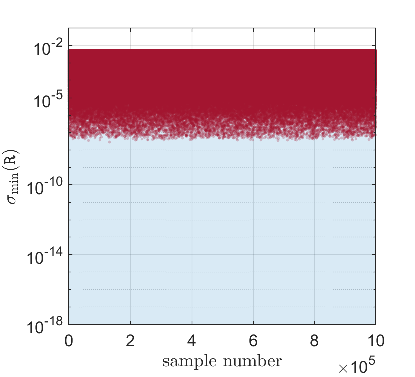
(a)

Figure 1: The smallest singular value (red dots) of the matrix $\mathtt{R}(\boldsymbol{P})$ of right eigenvectors of $\mathtt{A}(\boldsymbol{P})$.

Finally, remark that the analytical expressions of the eigenvalues and vectors are available for the case of stationary medium $\boldsymbol{v}_{1}=\boldsymbol{v}_{2}=0$. The eigenvalues are completely decoupled and read

$$\lambda_{1,2}=\pm C_{1}^{2},\qquad\lambda_{3,4}=\pm C_{2}^{2},\qquad\lambda_{5,6}=\pm\frac{\Sigma}{\rho}\sqrt{\|\boldsymbol{B}\|^{2}-B_{1}^{2}+\beta^{2}},\qquad\lambda_{7,\ldots,13}=0,$$ (34)

while the eigenvectors are linearly independent in this case.

6 Relaxation limit system via formal asymptotic analysis

System (17) contains a set of dissipative relaxation source terms with corresponding relaxation parameters. For some types of two-phase flows, such as dispersed flows (bubbly fluids, two-phase flows in porous media), a simplified model can be considered when assuming very fast (instantaneous) relaxation of the thermodynamic forces to the equilibrium. For example, the assumption of instantaneous pressure relaxation seems reasonable from a physical point of view, since the transition of the medium to an equilibrium state is determined by a few passages of fast pressure waves at the scale of dispersed inclusions. In many ways, the narrow mixing zone of a diffuse interface separating two fluids can be also considered as a dispersed zone, and therefore the above argument also applies.

In this section, we present a derivation of the so-called relaxation limit of equations (17) assuming instantaneous relaxation of all dissipative processes, namely relaxation of the microinertia thermodynamic force $E_{D}$, pressure $E_{\alpha}$, and relative velocity $E_{w_{k}}$.

First, considering $\varepsilon=\delta^{2}/\lambda\ll 1$ as a small parameter, we derive a relaxation limit for (17) assuming instantaneous relaxation of the thermodynamic force $E_{D}$ in Sec. 6.1. By these means, it will be demonstrated that in leading-orders in $\varepsilon$, the Young-Laplace law is fulfilled locally, in the mixture elements. Then, in Sec.6.2, we consider relaxation of the remaining thermodynamic forces $E_{\alpha}$ and $E_{w_{k}}$, and derive the final isentropic single-velocity approximation of (17).

6.1 Relaxation limit of (17)

For our purposes, it is enough to consider only two equations for $\alpha$ and $D$:

$$\rho\frac{\mathrm{d}\alpha}{{\mathrm{d}t}} =-\frac{1}{\delta}\rho E_{D},$$ (35a)

$$\rho\frac{\mathrm{d}D}{{\mathrm{d}t}}+\frac{\partial\left(\rho E_{B_{k}}\right)}{\partial x_{k}} =\frac{1}{\delta}\rho E_{\alpha}-\frac{1}{\varepsilon}\rho E_{D},$$ (35b)

where we have used the material time derivative $\mathrm{d}/{\mathrm{d}t}=\partial/\partial t+v_{k}\partial/\partial x_{k}$ to rewrite the equations in a more compact form.

We then expand $D$ and the thermodynamic force $E_{D}$

$$D =D_{0}+\epsilon D_{1}+\epsilon^{2}D_{2}+\ldots,$$ (36a)

$$E_{D} =E_{D,0}+\epsilon E_{D,1}+\epsilon^{2}E_{D,2}+\ldots,$$ (36b)

in powers of the small non-dimensional parameter $\epsilon=\varepsilon/\varepsilon_{0}$, where $\varepsilon_{0}$ is a time scale. Then, plugging this into (35b)

$$\rho\frac{\mathrm{d}}{{\mathrm{d}t}}\left(D_{0}+\epsilon D_{1}+\mathcal{O}(\epsilon^{2})\right)+\frac{\partial\left(\rho E_{B_{k}}\right)}{\partial x_{k}}=\frac{1}{\delta}\rho E_{\alpha}-\frac{1}{\varepsilon_{0}\epsilon}\rho\left(E_{D,0}+\epsilon E_{D,1}+\mathcal{O}(\epsilon^{2})\right),$$ (37)

we obtain that

$$E_{D,0}=\mathcal{O}(\epsilon).$$ (38)

Hence, assuming $E_{D,0}=0$ and $D_{0}=E_{D,0}/\beta^{2}=0$, we obtain the following approximate equation on $E_{D,1}$

$$\rho\frac{\mathrm{d}}{{\mathrm{d}t}}\left(\epsilon D_{1}+\mathcal{O}(\epsilon^{2})\right)+\frac{\partial\left(\rho E_{B_{k}}\right)}{\partial x_{k}}=\frac{1}{\delta}\rho E_{\alpha}-\frac{1}{\varepsilon_{0}\epsilon}\rho\left(\epsilon E_{D,1}+\mathcal{O}(\epsilon^{2})\right),$$ (39)

from which, we deduce that

$$E_{D,1}=\varepsilon_{0}\frac{1}{\delta}E_{\alpha}-\varepsilon_{0}\frac{1}{\rho}\frac{\partial}{\partial x_{k}}\left(\rho E_{B_{k}}\right)+\mathcal{O}(\epsilon).$$ (40)

On the other hand, the equation for $\alpha$ can be approximated as

$$\delta\rho\frac{\mathrm{d}\alpha}{{\mathrm{d}t}}=-\rho\epsilon E_{D,1}+\mathcal{O}(\epsilon^{2}),$$ (41)

and then, using the expression of $E_{D,1}$, the relaxation limit equation for volume fraction reads

$$\rho\frac{\mathrm{d}\alpha}{{\mathrm{d}t}}=-\frac{1}{\lambda}\rho E_{\alpha}+\frac{1}{\lambda}\delta\frac{\partial}{\partial x_{k}}\left(\rho E_{B_{k}}\right)+\mathcal{O}(\epsilon^{2}).$$ (42)

From this equation, we can conclude that, in contrast to the master system (1), the time evolution of the volume fraction is governed not only by the pressure relaxation $\lambda^{-1}\rho E_{\alpha}=\lambda^{-1}(p_{2}-p_{1})$, but also by the curvature of the diffuse interface. To see the latter, one needs to use the explicit expression of $E_{B_{k}}=\Sigma^{2}B_{k}/\rho^{2}$, the definition $B_{k}=\delta\frac{\partial\alpha}{\partial x_{k}}$, and the assumption that the surface tension coefficient $\sigma=\delta\Sigma^{2}/\rho$ is constant, $\sigma=const$. After this, equation (42) becomes (we omit the terms $\mathcal{O}(\epsilon^{2})$)

$$\rho\frac{\mathrm{d}\alpha}{{\mathrm{d}t}}=-\frac{1}{\lambda}\rho E_{\alpha}+\frac{1}{\lambda}\delta\sigma\frac{\partial}{\partial x_{k}}\left(\frac{\partial\alpha}{\partial x_{k}}\right),$$ (43)

where we used definition (27) of the surface tension coefficient $\sigma$.

In particular, for stationary flows ($\frac{\mathrm{d}\alpha}{{\mathrm{d}t}}=0$), the later equation reduces to

$$\delta\sigma\frac{\partial}{\partial x_{k}}\left(\frac{\partial\alpha}{\partial x_{k}}\right)=p_{2}-p_{1}.$$ (44)

To obtain the Young-Laplace law

$$\sigma\nabla\cdot\left(\frac{\nabla\alpha}{\|\nabla\alpha\ \|}\right)=p_{2}-p_{1},$$ (45)

from (44), the parameter $\delta=\|\nabla\alpha\|^{-1}$ must appear under the outer derivative $\partial/\partial x_{k}$, but $\delta$ is not constant and this cannot be done without altering (44). However, we shall show in Sec. 7, that in practical computations, $\delta$ can be replaced by an a priory computed constant (see (60)), so that in fact (44) approximates the Young-Laplace law (45).

Finally, we note that the relaxation limit of (17) for $\varepsilon\to 0$ is system (17) without equation for $D$ and in which the equations for $\alpha$ and $B_{k}$ are replaced by the following:

$$\rho\frac{\mathrm{d}\alpha}{{\mathrm{d}t}} -\frac{\delta}{\lambda}\frac{\partial}{\partial x_{k}}\left(\rho E_{B_{k}}\right)=-\frac{1}{\lambda}\rho E_{\alpha},$$ (46a)

$$\frac{\mathrm{d}B_{k}}{{\mathrm{d}t}} +B_{j}\frac{\partial v_{j}}{\partial x_{k}}+\frac{\partial}{\partial x_{k}}\left(\frac{\delta}{\lambda}E_{\alpha}\right)-\frac{\partial}{\partial x_{k}}\left(\frac{\delta^{2}}{\lambda\rho}\frac{\partial\rho E_{B_{j}}}{\partial x_{j}}\right)=0,$$ (46b)

where the equation for $B_{k}$ is a second order parabolic equation, that can be obtained by the same means as (42).

One could note the antisymmetric structure (opposite signs) of the constitutive fluxes in (46) involving the thermodynamic forces $E_{\alpha}$ and $E_{B_{k}}$. This usually results in complex eigenvalues, and subsequently in the loss of hyperbolicity of the first-order differential operator (without dissipative parabolic term in the second equation of (46)). Therefore, in the next section we consider another relaxation limit of (17), in which we couple the result of this section with the single velocity approximation ($\boldsymbol{v}_{1}=\boldsymbol{v}_{2}$).

6.2 Relaxation limit of the single velocity isentropic model

In this section, on top of the previous result, we derive reduced single-velocity isentropic equations obtained as a relaxation limit of (17) when $E_{\alpha}$ and $E_{w_{k}}$ are instantaneously set to their equilibrium values. The latter can be obtained by simply assuming the relative velocity to be zero $\boldsymbol{w}=\boldsymbol{v}_{1}-\boldsymbol{v}_{2}=0$, since $E_{\boldsymbol{w}}=c(1-c)\boldsymbol{w}$. Thus, the single-velocity approximation system is a consequence of (17) under the assumption $w_{k}=0$, that can be written in the following form

$$\frac{\partial\rho_{1}\alpha_{1}}{\partial t}+\frac{\partial\rho_{1}\alpha_{1}v_{k}}{\partial x_{k}}=0,$$ (47a)

$$\frac{\partial\rho_{2}\alpha_{2}}{\partial t}+\frac{\partial\rho_{2}\alpha_{2}v_{k}}{\partial x_{k}}=0,$$ (47b)

$$\frac{\partial\rho v_{i}}{\partial t}+\frac{\partial\left(\rho v_{i}v_{k}+\rho^{2}E_{\rho}\delta_{ki}+\rho B_{i}E_{B_{k}}\right)}{\partial x_{k}}=0,$$ (47c)

$$\frac{\partial\rho\alpha}{\partial t}+\frac{\partial\rho\alpha v_{k}}{\partial x_{k}}=-\frac{1}{\delta}\rho E_{D},$$ (47d)

$$\frac{\partial\rho D}{\partial t}+\frac{\partial(\rho Dv_{k}+\rho E_{B_{k}})}{\partial x_{k}}=\frac{1}{\delta}\rho E_{\alpha}-\frac{1}{\varepsilon}\rho E_{D},$$ (47e)

$$\frac{\partial B_{k}}{\partial t}+\frac{\partial(B_{l}v_{l}+E_{D})}{\partial x_{k}}+v_{l}\left(\frac{\partial B_{k}}{\partial x_{l}}-\frac{\partial B_{l}}{\partial x_{k}}\right)=0.$$ (47f)

In the previous section, we derived the asymptotic equation (42) for the volume fraction assuming small relaxation time for the microinertia field $D$. In turn, further assuming that the relaxation parameter $\lambda$ is sufficiently small so that the time variation of the volume fraction is small in comparison with the relaxation rate $\lambda^{-1}$, equation (42) can be approximated as

$$p_{2}(\rho_{2})-p_{1}(\rho_{1})={\delta}\frac{\partial\rho E_{B_{k}}}{\partial x_{k}}.$$ (48)

From (48), we immediately obtain two relations for derivatives of phase mass densities

$$C^{2}_{2}\frac{\partial\rho_{2}}{\partial t}-C^{2}_{1}\frac{\partial\rho_{1}}{\partial t}=\frac{\partial}{\partial t}\left({\delta}\frac{\partial\rho E_{B_{k}}}{\partial x_{k}}\right),\qquad C^{2}_{2}\frac{\partial\rho_{2}}{\partial x_{j}}-C^{2}_{1}\frac{\partial\rho_{1}}{\partial x_{j}}=\frac{\partial}{\partial x_{j}}\left({\delta}\frac{\partial\rho E_{B_{k}}}{\partial x_{k}}\right),$$ (49)

where $C_{a}^{2}=\partial p_{a}/\partial\rho_{a}$, $a=1,2$ are the phase adiabatic sound speeds.

Now, using relations (49) and phase mass conservation equations (47a), (47b), one can obtain the following equation for $\alpha_{1}$:

$$\frac{\mathrm{d}\alpha_{1}}{{\mathrm{d}t}}+\frac{\alpha_{1}\alpha_{2}(K_{1}-K_{2})}{\alpha_{2}K_{1}+\alpha_{1}K_{2}}\frac{\partial v_{k}}{\partial x_{k}}-\frac{\alpha_{1}\alpha_{2}}{\alpha_{2}K_{1}+\alpha_{1}K_{2}}\frac{\mathrm{d}}{{\mathrm{d}t}}\left({\delta}\frac{\partial\rho E_{B_{k}}}{\partial x_{k}}\right)=0,$$ (50)

where $K_{a}=\rho_{a}C_{a}^{2}$ are the phase bulk moduli.

If we recall the definition $B_{k}=\delta\partial\alpha_{1}/\partial x_{k}$, then it is clear that (50) is a third-order partial differential equation for $\alpha=\alpha_{1}$. Finally, we can also formulate a closed relaxation limit system of the single velocity isentropic approximation of (17) for the variables $\alpha_{1}$, $\rho_{1}$, $\rho_{2}$, and $v_{k}$:

$$\frac{\partial\alpha_{1}}{\partial t}+v_{k}\frac{\partial\alpha_{1}}{\partial x_{k}}+\frac{\alpha_{1}\alpha_{2}(K_{1}-K_{2})}{\alpha_{2}K_{1}+\alpha_{1}K_{2}}\frac{\partial v_{k}}{\partial x_{k}}-\frac{\alpha_{1}\alpha_{2}}{\alpha_{2}K_{1}+\alpha_{1}K_{2}}\frac{\mathrm{d}}{{\mathrm{d}t}}\left(\delta\sigma\frac{\partial^{2}\alpha_{1}}{\partial x_{k}\partial x_{k}}\right)=0,$$ (51a)

$$\frac{\partial\rho_{1}\alpha_{1}}{\partial t}+\frac{\partial\rho_{1}\alpha_{1}v_{k}}{\partial x_{k}}=0,$$ (51b)

$$\frac{\partial\rho_{2}\alpha_{2}}{\partial t}+\frac{\partial\rho_{2}\alpha_{2}v_{k}}{\partial x_{k}}=0,$$ (51c)

$$\frac{\partial\rho v_{i}}{\partial t}+\frac{\partial}{\partial x_{k}}\left(\rho v_{i}v_{k}+\left(p_{1}+\alpha_{2}\left(\delta\sigma\frac{\partial^{2}\alpha_{1}}{\partial x_{j}\partial x_{j}}\right)\right)\delta_{ki}+\hat{T}_{ki}\right)=0,$$ (51d)

where $\hat{T}_{ki}=-\frac{\Sigma^{2}}{\rho}\left(B_{j}B_{j}\delta_{ki}-B_{k}B_{i}\right)$ is the surface tension stress tensor which should also be expressed in terms of the gradients $\partial\alpha_{1}/\partial x_{k}$ using the definition of $B_{k}$.

Note that if surface tension is neglected, then terms with higher derivatives of $\alpha_{1}$ and the tensor $\hat{T}_{ki}$ should be excluded from (51). In this case, (51) transforms to the well-known five-equation two-phase model of Kapila [33].

The presence of third-order derivatives in (51) and the corresponding dispersion effects of the model can lead to non-standard behavior of waves and this will be the subject of further research.

7 Stationary solution of a spherical bubble

In the previous section, we demonstrated that in the limit $\delta\to 0$ and $\lambda\to 0$, in the leading-order terms, the pressure difference inside a mixture element fulfills the relation (44), that in turn resembles the Young-Laplace law (45). The formal obstacle to identify the two relations (44) and (45) is the parameter $\delta=\|\nabla\alpha\|^{-1}$ that appears outside of the divergence operator. In what follows, we shall demonstrate that, in fact, $\delta$ can be chosen as a constant so that the Young-Laplace law holds on macroscopic diffuse interfaces between two immiscible fluids in an approximation sense.

We shall search for a spherically symmetric stationary solution to system (17) representing a bubble or droplet of a radius $R$. Thus, we assume that $\boldsymbol{v}=0$ and $\boldsymbol{w}=0$. We also assume that the temperature variations are negligible, that means that we can exclude the entropy from consideration. All unknown scalar functions can be parameterized as

$$\alpha(t,\boldsymbol{x})=\tilde{\alpha}(r),\qquad\rho(t,\boldsymbol{x})=\tilde{\rho}(r),\qquad D(t,\boldsymbol{x})=\tilde{D}(r),\qquad r=\|\boldsymbol{x}\|$$ (52)

and vector fields as

$$B_{k}(t,\boldsymbol{x})=\tilde{B}(r)\frac{x_{k}}{r}.$$ (53)

Moreover, we prescribe the distribution of $\tilde{\alpha}$ in the diffuse interface between the fluids in the form

$$\tilde{\alpha}(r)=\frac{1}{2}\left(1-\tanh\left(\frac{\pi(r-R)}{h}\right)\right),$$ (54)

where $h$ is the thickness of the diffuse interface, and we will look for a solution that satisfy (54). This also fixes $\tilde{B}(r)$ as

$$\tilde{B}(r)=\delta\tilde{\alpha}^{\prime}(r)$$ (55)

due to the definition (15) of the vector field $B_{k}$. In the following, we shall omit the tilde sign “$\tilde{\phantom{\alpha}}$” above the unknowns for simplicity of notations. The reader should keep in mind that all the state variables are functions of the single variable $r$.

It is sufficient to consider the momentum equations and equation on $D$ that, for a steady state, reduce to

$$\frac{\partial(\rho^{2}E_{\rho}\delta_{ki}+\rho B_{i}E_{B_{k}})}{\partial x_{k}}=0,\quad i=1,2,3,$$ (56a)

$$\frac{\partial(\rho E_{B_{k}})}{\partial x_{k}}=\frac{1}{\delta}\rho E_{\alpha}.$$ (56b)

After using the spherical symmetry assumptions (53), definition of $B(r)$ (55), and the relation $\sigma=\delta\Sigma^{2}/\rho$ (27), these two equations reduce to an ordinary differential equation and an algebraic equation (because $\alpha(r)$ is given by (54))

$$p^{\prime}(r) =-\frac{2\sigma\delta(r)\alpha^{\prime}(r)^{2}}{r}\equiv F(r),$$ (57a)

$$p_{2}(r)-p_{1}(r) =\sigma\delta(r)\left(\frac{d-1}{r}\alpha^{\prime}(r)+\alpha^{\prime\prime}(r)\right)\equiv G(r),$$ (57b)

where $d$ is the space dimension ($d=3$ in this example).

The first equation can be integrated to get the mixture pressure $p(r)=\alpha(r)p_{1}(r)+(1-\alpha(r))p_{2}(r)$

$$p(r)=p_{\textrm{atm}}-\int\limits_{r}^{\infty}F(\zeta)\mathrm{d}\zeta,\qquad p_{\textrm{atm}}=p(\infty),$$ (58)

after which, the phase pressures can be found as

$$p_{1}(r)=p(r)-(1-\alpha(r))G(r),\qquad p_{2}(r)=p(r)+\alpha(r)G(r).$$ (59)

In Section 4, we concluded that to recover the conventional capillary stress tensor (26), one should take $\delta(r)=\|\nabla\alpha\|^{-1}$. This, however, is not convenient from the computational view point, because $\nabla\alpha$ is not a state variable of the system (17) and cannot be easily evaluated. Therefore, a practical procedure has to be invented in order to provide a reasonable estimate of $\delta$ a priori. In this paper, we suggest replacing $\delta(r)$ by the following constant $\delta_{0}=\text{const}$

$$\delta_{0}(h)=\int\limits_{R-h}^{R+h}r^{-1}\alpha^{\prime}(r)\mathrm{d}r\cdot\left(\int\limits_{R-h}^{R+h}r^{-1}\alpha^{\prime}(r)^{2}\mathrm{d}r\right)^{-1},$$ (60)

which is choosing in such a way to obtain the Young-Laplace formula $\Delta p=-2\sigma/R$ in (57a). Exactly this $\delta_{0}$ is used instead of $\delta=\|\nabla\alpha\|^{-1}$ in the numerical results below.

Typical solutions to (58) for $R=0.01$, $\sigma=0.0728$, and various interface widths $h$ are depicted in Fig. 2. In particular, one can see that as long as $h\to 0$ the pressure jump across the interface converges to the theoretical one $\Delta p_{\textrm{theor}}=(d-1)\sigma/R=14.56$ given by the Young-Laplace law. One should bear in mind that for every curve in Fig. 2, $\delta_{0}(h)$ is different since it depends on $h$.

Fig. 3 depicts the phase pressure $p_{a}(r)$ and partial pressure $\hat{p}_{a}(r)=\alpha_{a}(r)p_{a}(r)$ variations across the interface. It demonstrates the main feature of our model, that is, the pressures $p_{1}$ and $p_{2}$ of the mixture constituents can be different, and that the presence of the interface curvature prevent $p_{1}$ and $p_{2}$ from relaxing to a common value as it is assumed in the single-pressure models, e.g. [4, 38, 56, 9].

For this particular solution, one does not need to specify the fluid equations of state $e_{a}(\rho_{a},S)$ in (23), however, it would be interesting to take some particular internal energies $e_{a}(\rho_{a},S)$ and to look at the density variation across the interface. Thus, we shall assume that the fluid with index $a=1$ (in the center of the domain, left from the interface in the figures) is an ideal gas given by the ideal gas equation of state, while the fluid $a=2$ is a liquid parameterized by the stiffened-gas equation of state

$$e_{1}(\rho_{1},S)=\frac{c_{10}^{2}}{\gamma_{1}(\gamma_{1}-1)}\left(\frac{\rho_{1}}{\rho_{10}}\right)^{\gamma_{1}-1}e^{S/c_{V,1}},\qquad e_{2}(\rho_{2},S)=\frac{c_{20}^{2}}{\gamma_{2}(\gamma_{2}-1)}\left(\frac{\rho_{2}}{\rho_{20}}\right)^{\gamma_{2}-1}e^{S/c_{V,2}}+\frac{\rho_{20}c_{20}^{2}-\gamma_{2}p_{20}}{\gamma_{2}\rho_{2}},$$ (61)

where $c_{V,a}$, $a=1,2$ are the specific heats at constant volume, $\gamma_{a}$ are the ratio of the specific heats, $c_{a0}$ are the reference sound speeds, $\rho_{a0}$ are the reference phase mass densities, and $p_{20}$ is the reference pressure of the liquid phase.

Fig. 4 shows typical density profiles recovered from the pressure profiles using equations of state (61). The following values were used for the gas phase $\gamma_{1}=1.4$, $c_{10}=343.03$, $c_{V,1}=717.2$, $S=0$ that gives the equilibrium density of the gas $\rho_{10}=1.205$. The liquid parameters were taken as follows $\gamma_{2}=1.949437$, $c_{V,2}=4150$, $p_{20}=p_{\textrm{atm}}=101325$, $c_{20}=1500$, $\rho_{20}=1000$. Computing the phase pressures as $p_{a}=\rho_{a}^{2}\frac{\partial e_{a}}{\partial\rho_{a}}$ and inverting it with respect to $\rho_{a}$, we can plot the density profiles as depicted in Fig. 4. Note that the liquid density $\rho_{2}(r)$ is not exactly constant as it may seem from Fig. 4 (middle) but its perturbations are of the order $10^{-8}$.

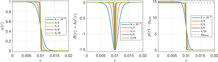
(a)

Figure 2: Diffuse interface profile for the stationary bubble of radius $R=0.01$, $\sigma=0.0728$ for which the theoretical pressure jump $\Delta p_{\textrm{theor}}=(d-1)\sigma/R=14.56$. Left: volume fraction for various interface width $h$. Right: mixture pressure $p(r)=\alpha p_{1}+(1-\alpha)p_{2}$

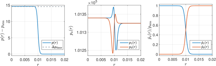
(a)

Figure 3: Mixture pressure $p(r)$ (left), phase pressures $p_{a}(r)$ (middle), and partial pressures $\hat{p}_{a}(r)=\alpha_{a}p_{a}$ (right), for a stationary bubble with $R=0.01$, $\sigma=0.0728$, and $h=0.005$.

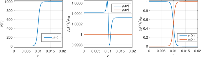
(a)

Figure 4: Mixture mass density $\rho(r)=\alpha\rho_{1}+(1-\alpha)\rho_{2}$ (left), phase mass densities $\rho_{a}(r)$ (middle), and apparent densities $\varrho_{a}(r)=\alpha_{a}\rho_{a}$ (right), for a stationary bubble with $R=0.01$, $\sigma=0.0728$, and $h=0.005$. The ideal gas and stiffened-gas equations of state were used to obtain fluid densities $\rho_{a}$ from pressures $p_{a}$.

8 Dispersion relations

In this section, we perform a linear stability analysis of (17) by considering a particular solution in the form of a plane wave

$$\boldsymbol{Q}(t,\boldsymbol{x})=\boldsymbol{Q}_{0}e^{i(\omega t-\boldsymbol{k}\cdot\boldsymbol{x})},$$ (62)

where $i=\sqrt{-1}$ is the imaginary unit, $\omega=2\pi f$ is the real angular frequency, $f$ is the frequency, $\boldsymbol{k}$ is the complex wave vector. It is sufficient to restrict the analysis to the 1D case, i.e. $\boldsymbol{x}=(x,0,0)$, and $\boldsymbol{k}=(k,0,0)$, and moreover to the genuinely 1D case, i.e. we set $(v_{a,1},v_{a,2},v_{a,3})=(v_{a},0,0)$, $(B_{1},B_{2},B_{3})=(B,0,0)$.

To derive the required PDE system it is necessary to use relations between mixture and individual phases variables of state. Then, after a cumbersome but standard procedure, one can derive equations for the state variables of the phases and linearize these equations near the equilibrium state $v_{a}=0+v^{\prime}_{a}$, $\rho_{a}=\rho_{a,0}+\rho^{\prime}_{a}$, $\alpha=\alpha_{0}+\alpha^{\prime}$, $D=0+D^{\prime}$, $B=B_{0}+B^{\prime}$.

The equations for perturbations $\boldsymbol{Q}^{\prime}=(v^{\prime}_{1},v^{\prime}_{2},B^{\prime},D^{\prime},\alpha^{\prime},\rho^{\prime}_{1},\rho^{\prime}_{2})$ reads (we omit the prime symbol “$\,{}^{\prime}\,$” for the sake of brevity)

$$\frac{\partial v_{1}}{\partial t}+\frac{p_{1,0}-p_{2,0}}{\rho_{0}}\frac{\partial\alpha}{\partial x}+\frac{C_{1}^{2}}{\rho_{1,0}}\frac{\partial\rho_{1}}{\partial x}=-\frac{c_{1,0}c_{2,0}^{2}}{\chi}\left(v_{1}-v_{2}\right),$$ (63a)

$$\frac{\partial v_{2}}{\partial t}+\frac{p_{1,0}-p_{2,0}}{\rho_{0}}\frac{\partial\alpha}{\partial x}+\frac{C_{2}^{2}}{\rho_{2,0}}\frac{\partial\rho_{2}}{\partial x}=+\frac{c_{1,0}^{2}c_{2,0}}{\chi}\left(v_{1}-v_{2}\right),$$ (63b)

$$\frac{\partial B}{\partial t}+B_{0}c_{1,0}\frac{\partial v_{1}}{\partial x}+B_{0}c_{2,0}\frac{\partial v_{2}}{\partial x}+\beta^{2}\frac{\partial D}{\partial x}=0,$$ (63c)

$$\frac{\partial D}{\partial t}+\frac{\Sigma^{2}}{\rho_{0}^{2}}\frac{\partial B}{\partial x}-\frac{B_{0}\Sigma^{2}\left(\rho_{1,0}-\rho_{2,0}\right)}{\rho_{0}^{3}}\frac{\partial\alpha}{\partial x}-\frac{\alpha_{0}B_{0}\Sigma^{2}}{\rho_{0}^{3}}\frac{\partial\rho_{1}}{\partial x}-\frac{\left(1-\alpha_{0}\right)B_{0}\Sigma^{2}}{\rho_{0}^{3}}\frac{\partial\rho_{2}}{\partial x}=-\frac{\rho_{1}C_{1,0}^{2}-\rho_{2}C_{2,0}^{2}}{\delta\rho_{0}}-\frac{\beta^{2}\lambda}{\delta^{2}}D,$$ (63d)

$$\frac{\partial\alpha}{\partial t}=-\frac{\beta^{2}}{\delta}D,$$ (63e)

$$\frac{\partial\rho_{1}}{\partial t}+\rho_{1}\frac{\partial v_{1}}{\partial x}=\frac{\beta^{2}\rho_{1,0}}{\alpha_{0}\delta}D,$$ (63f)

$$\frac{\partial\rho_{2}}{\partial t}+\rho_{2}\frac{\partial v_{2}}{\partial x}=-\frac{\beta^{2}\rho_{2,0}}{\left(1-\alpha_{0}\right)\delta}D,$$ (63g)

where $C_{a}^{2}=\frac{\partial p_{a}}{\partial\rho_{a}}$, $a=1,2$

If linear system (63) is written in the matrix notations as

$$\boldsymbol{Q}_{t}+\mathtt{A}\boldsymbol{Q}_{x}=\mathtt{S}\boldsymbol{Q}$$ (64)

then the dispersion relations $k(\omega)$ of (63) are given as the roots of the polynomial (e.g. see [32])

$$\det\left(\mathtt{I}-\frac{k}{\omega}\mathtt{A}+\frac{i}{\omega}\mathtt{S}\right)=0,$$ (65)

with $\mathtt{I}$ being the identity matrix.

The phase $V_{\text{ph}}(\omega)$ and group $V_{\text{g}}(\omega)$ velocities and the attenuation factor $A(\omega)$ can be computed as

$$V_{\text{ph}}=\frac{\omega}{\text{Re}(k)},\qquad V_{\text{g }}=\left(\frac{\partial\text{Re}(k)}{\partial\omega}\right)^{-1},\qquad A(\omega)=-\text{Im}(k).$$ (66)

The polynomial (65) is a cubic polynomial on $k(\omega)^{2}$, and its roots correspond to three modes: the pressure modes of the two phases, and the capillarity mode associated with the surface tension. All three modes are stable as can be seen from the attenuation factors plotted in Fig. 5–7 and which are positive.

Figures 5–7 show typical dispersion curves for the thermodynamic parameters extracted from the stationary bubble solution corresponding to $\alpha=0.999$ (almost pure gas), $\alpha=0.519$ (mixed state), $\alpha=0.002$ (almost pure liquid). The curves are plotted along side with the phase characteristic velocities $C_{a}^{2}=\frac{\partial p_{a}}{\partial\rho_{a}}$, the so-called equilibrium sound speed $C_{\text{e}}$ and Wood’s sound speed $C_{\text{W}}$ (dashed lines) given by [18]

$$C_{\text{e}}^{2}=\left(\rho\left(\frac{\alpha_{1}}{\rho_{1}C_{1}^{2}}+\frac{\alpha_{2}}{\rho_{2}C_{2}^{2}}\right)\right)^{-1},\qquad C_{\text{W}}^{2}=C_{1}^{2}C_{2}^{2}\left(\frac{\rho_{1}}{\alpha_{1}}+\frac{\rho_{2}}{\alpha_{2}}\right)\left(\frac{\rho_{1}C_{1}^{2}}{\alpha_{1}}+\frac{\rho_{2}C_{2}^{2}}{\alpha_{2}}\right)^{-1}.$$ (67)

From these figures, one can note that Wood’s speed $C_{\text{W}}$ serves as a low frequency limit for the sound speed of the gaseous phase $a=1$ (the light one), and the equilibrium speed $C_{\text{e}}$ is the high-frequency limit of the gaseous phase.

On the other hand, the liquid phase (the heavy one), has $C_{2}$ as the high-frequency limit, while its low-frequency limit is undetermined in general.

The most interesting behavior of the sound waves can be seen in Fig. 7 corresponding to $\alpha=0.00206$ that can be considered as if a gaseous phase $\rho_{1}=1.205$ is dispersed in a heavy liquid phase $\rho_{2}=1000$. Thus, the velocity of the sound mode corresponding to the light phase may change from $C_{\text{W}}=258.7$ at $\omega\to 0$ to $C_{1}=343.1$ at $\omega\to\infty$ through $C_{\text{e}}=425.3$ at moderate frequencies.

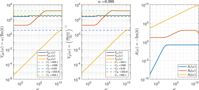
(a)

Figure 5: Phase velocities (left), group velocities (middle), and attenuation factor (right) versus the angular frequency $\omega=2\pi f$, where $f$ is the frequency. The dashed lines shows the pure gas $C_{1}=\sqrt{\partial p_{1}(\rho_{1},S)/\partial\rho_{1}}$ and liquid $C_{2}=\sqrt{\partial p_{2}(\rho_{2},S)/\partial\rho_{2}}$ characteristic velocities, equilibrium characteristic speed $C_{\text{e}}$, and Wood’s sound speed $C_{\text{W}}$. The mixture parameters are $\alpha=0.999$, $\beta=1$, $\delta=0.0025$, $\delta/\lambda=10^{-8}$. The phase pressures parameters are extracted from the stationary bubble solution at the corresponding value of $\alpha$: $p_{1}=p_{2}=1.013395\cdot 10^{5}$, while other thermodynamic parameters were computed from the equations of state.

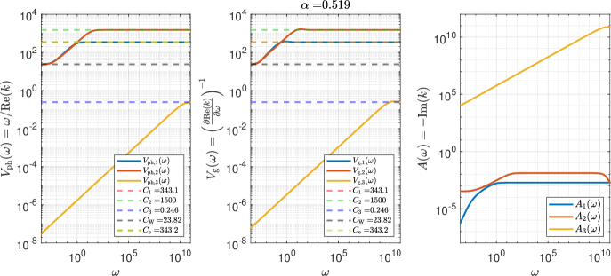
(a)

Figure 6: Phase velocities (left), group velocities (middle), and attenuation factor (right) versus the angular frequency $\omega=2\pi f$, where $f$ is the frequency. The dashed lines shows the pure gas $C_{1}=\sqrt{\partial p_{1}(\rho_{1},S)/\partial\rho_{1}}$ and liquid $C_{2}=\sqrt{\partial p_{2}(\rho_{2},S)/\partial\rho_{2}}$ characteristic velocities, equilibrium characteristic speed $C_{\text{e}}$, and Wood’s sound speed $C_{\text{W}}$. The mixture parameters are $\alpha=0.519$, $\beta=1$, $\delta=0.0025$, $\delta/\lambda=10^{-8}$. The phase pressures parameters are extracted from the stationary bubble solution at the corresponding value of $\alpha$: $p_{1}=1.013531\cdot 10^{5}$, $p_{2}=1.013103\cdot 10^{5}$, while other thermodynamic parameters were computed from the equations of state.

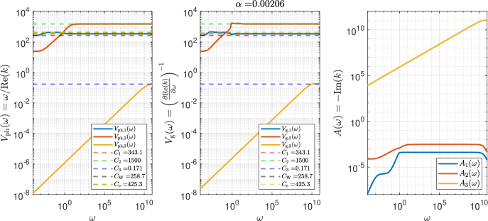
(a)

Figure 7: Phase velocities (left), group velocities (middle), and attenuation factor (right) versus the angular frequency $\omega=2\pi f$, where $f$ is the frequency. The dashed lines shows the pure gas $C_{1}=\sqrt{\partial p_{1}(\rho_{1},S)/\partial\rho_{1}}$ and liquid $C_{2}=\sqrt{\partial p_{2}(\rho_{2},S)/\partial\rho_{2}}$ characteristic velocities, equilibrium characteristic speed $C_{\text{e}}$, and Wood’s sound speed $C_{\text{W}}$. The mixture parameters are $\alpha=0.00206$, $\beta=1$, $\delta=0.0025$, $\delta/\lambda=10^{-8}$. The phase pressures parameters are extracted from the stationary bubble solution at the corresponding value of $\alpha$: $p_{1}=1.0132276\cdot 10^{5}$, $p_{2}=1.0132500\cdot 10^{5}$, while other other thermodynamic parameters were computed from the equations of state.

9 Conclusion

We have presented a new nonequilibrium two-pressure diffuse interface model for two-fluid systems with surface tension. The model represents an extension of the SHTC two-fluid mixture model [51, 52, 46, 45] in which the time and space gradients of the volume fraction are lifted to the level of state variables to account for spatial heterogeneities and microinertial effect in the vicinity of the diffuse interface. The resulting model belongs to the class of thermodynamically compatible hyperbolic equations for which both laws of thermodynamics hold.

The main difference from the existing diffuse interface approaches to surface tension such as [4, 38, 56, 9] is that the pressure equilibrium condition $p_{1}=p_{2}$ is not assumed in our model. The pressure non-equilibrium is actually a fundamental assumption for introduction of the surface tension into the two-fluid SHTC model in order to gain the full SHTC structure of the governing equations. In particular, it is important for the variational and Hamiltonian formulations of the governing equations discussed in Sec. A and B.

We presented two reduced relaxation limits of the model. In Sec. 6.1, the relaxation limit of the equations when the microinertia relaxation rate is very fast. In Sec.6.2, the relaxation limit for very fast pressure and velocity relaxation rates was derived that can be called single-velocity pressure-equilibrium model. These reduced models can be used for better understanding of the solution properties of the full system. In particular, we demonstrated that the Young-Laplace law is approximately holds in a mixture element as long as the gradient of the volume fraction is not equal to zero. Furthermore, the single-velocity pressure-equilibrium reduced model is a system of third-order partial differential equations which can be used to connect our model to some classical dispersive models. The dispersion relation of the full model can be obtained numerically and was studied in Sec.8. The full model has three modes: two pressure modes of the constituents and the third mode, related to the microinertia of the interface. The analysis revealed non trivial dependencies of the phase velocities on frequency.

Although we could not conduct the hyperbolicity analysis of the full system completely, our preliminary study suggests that the full two-fluid model with surface tension is hyperbolic at least in the vicinity of equilibrium. Also, during this research, we found out that the energy potential is not strictly convex and thus formally the model does not have all properties of the SHTC class of equations. We shall address this issue in more detail in future.

Finally, we studied the stationary bubble solution, and demonstrated that the Young-Laplace law holds as a sharp interface limit for macroscopic interfaces. Although the new parameter $\delta$ is not a constant, from the theoretical viewpoint, and must be chosen as $\delta=\|\nabla\alpha\|^{-1}$, we demonstrated that in practical computations it can be taken as a precomputed constant, see (60).

In future, we shall extend the model so that it applies also to complex fluids and solids, such as superfluid helium-4 or non-Newtonian fluids.

Appendix A Variational formulation

Here we briefly recall the variational scheme that underlies every SHTC equations, see [40]. The variational principle is formulated in the Lagrangian coordinates $\boldsymbol{X}=\left\{X^{K}\right\}$, $K=1,2,3$. For simplicity, we only consider the surface tension part.

Thus, we consider a general Lagrangian density $\Lambda=\Lambda(\alpha,\phi,\beta_{K})$ which is a function of the volume fraction and their space and time gradients

$$\phi:=\mathrm{d}_{t}\alpha,\qquad\beta_{K}:=\partial_{K}\alpha,$$ (68)

where $\mathrm{d}_{t}=\mathrm{d}/{\mathrm{d}t}$ is the material time derivative and $\partial_{K}=\partial/\partial X^{K}$. Hence, varying the action integral

$$\mathcal{A}=\int\Lambda(\alpha,\mathrm{d}_{t}\alpha,\partial_{K}\alpha){\mathrm{d}t}\mathrm{d}\boldsymbol{X}$$ (69)

with respect to $\delta\alpha$, one immediately obtains the Euler-Lagrange equation

$$\frac{\mathrm{d}\Lambda_{\phi}}{{\mathrm{d}t}}+\frac{\partial\Lambda_{\beta_{K}}}{\partial X^{K}}=\Lambda_{\alpha},$$ (70)

where $\Lambda_{\alpha}=\frac{\partial\Lambda}{\partial\alpha}$, $\Lambda_{\phi}=\frac{\partial\Lambda}{\partial\phi}$, and $\Lambda_{\beta_{K}}=\frac{\partial\Lambda}{\partial\beta_{K}}$. The Euler-Lagrange equation is formally a second-order PDE for $\alpha$. To obtain an extended first-order system for $\left\{\alpha,\phi,\beta_{K}\right\}$ as required by the SHTC theory, we need to provide an evolution equations for the vector $\beta_{K}$ and $\alpha$ which is in fact not a difficult task because these equations are trivial consequences of the definitions of $\beta_{K}$ and $\phi$. Indeed, the required system of first-order PDEs reads

$$\frac{\mathrm{d}\Lambda_{\phi}}{{\mathrm{d}t}} +\frac{\partial\Lambda_{\beta_{K}}}{\partial X^{K}}=\Lambda_{\alpha},$$ (71a)

$$\frac{\mathrm{d}\beta_{K}}{{\mathrm{d}t}} -\frac{\partial\phi}{\partial X^{K}}=0,$$ (71b)

$$\frac{\mathrm{d}\alpha}{{\mathrm{d}t}} =\phi.$$ (71c)

By introducing new potential as a partial Legendre transform of $\Lambda$

$$U(\alpha,d,b_{K}):=\phi\Lambda_{\phi}-\Lambda,$$ (72)

and new variables

$$d:=\Lambda_{\phi},\qquad b_{K}:=-\beta_{K},$$ (73)

system (71) can be rewritten as

$$\frac{\mathrm{d}d}{{\mathrm{d}t}} +\frac{\partial U_{b_{K}}}{\partial X^{K}}=-U_{\alpha},$$ (74a)

$$\frac{\mathrm{d}b_{K}}{{\mathrm{d}t}} +\frac{\partial U_{d}}{\partial X^{K}}=0,$$ (74b)

$$\frac{\mathrm{d}\alpha}{{\mathrm{d}t}} =U_{d},$$ (74c)

where we have used the standard properties of the Legendre transform

$$U_{\alpha}=-\Lambda_{\alpha},\qquad\phi=U_{d}.$$ (75)

Finally, performing the Lagrange-to-Euler transformation of the energy potential, state variables, and time and space derivatives

$$A^{K}_{\ i}:=\frac{\partial X^{K}}{\partial x^{i}},\qquad\frac{\partial}{\partial x^{i}}=A^{K}_{\ i}\frac{\partial}{\partial X^{k}},\qquad\frac{\mathrm{d}}{{\mathrm{d}t}}=\frac{\partial}{\partial t}+v^{k}\frac{\partial}{\partial x^{k}},$$ (76a)

$$E:=\det(\boldsymbol{A})U,\qquad d:=\det(\boldsymbol{A})d,\qquad b_{i}:=A^{K}_{\ i}b_{k},$$ (76b)

$$\frac{\mathrm{d}}{{\mathrm{d}t}}A^{K}_{\ i}+A^{K}_{\ j}\frac{\partial v^{j}}{\partial x^{i}}=0$$ (76c)

as detailed in [40], equations (74) become (14). Note that, in (74a), an equivalent of the source term $\lambda\rho E_{d}$ in (14b) is missing because it is a dissipative term and cannot be included into the variational scheme but must be added afterwards in correspondence with the second law of thermodynamics [40].

Appendix B Hamiltonian formulation

Equations (17) consist of a reversible part and an irreversible part (the two source terms with the rates $\chi^{-1}$ and $\varepsilon^{-1}$). The purpose of this Section is to show that the reversible part has a Hamiltonian structure, meaning that it is generated by a Poisson bracket. This underlines the internal consistency of the equations and provides to them an alternative geometric interpretation [36].

Poisson brackets are a cornerstone of analytical mechanics [21], where they typically come out of variation of action. Then, they come in the so-called canonical form for the pairs of coordinates and their respective momenta. But in continuum mechanics, which is the case here, Poisson brackets are typically non-canonical, they are degenerate, and do not need to have state variables in the form of pairs of coordinates and momenta [10, 2, 14, 36].

In general, Poisson brackets are bilinear operators from a space of functionals of some state variables $\boldsymbol{q}$ to the same space. Moreover, they are skew-symmetric, $\{F,G\}=-\{G,F\}$, for each two functionals $F(\boldsymbol{q})$ and $G(\boldsymbol{q})$, and they satisfy the Leibniz rule and Jacobi identity. The state variables can be for instance positions and momenta, which is the usual case in analytical mechanics, but also fields as density, momentum density, and others. The Leibniz rule, $\{F,GH\}=\{F,G\}H+G\{F,H\}$ means that Poisson brackets behave as derivatives, which in particular means that the resulting evolution equations do not depend on constant shifts of energy. Finally, Jacobi identity, $\{F,\{G,H\}+\{G,\{H,F\}+\{H,\{F,G\}=0$, expresses self-consistency of Hamiltonian mechanics [16, 37]. Once the Poisson bracket for a state variable vector $\boldsymbol{q}$ is determined, Hamiltonian evolution of $\boldsymbol{q}$ is given by

$$\dot{\boldsymbol{q}}=\{\boldsymbol{q},\mathcal{E}\},$$ (77)

where $\mathcal{E}=\int e(\boldsymbol{q})d\boldsymbol{x}$ is the total energy of the system and $e(\boldsymbol{q})$ the volumetric energy density.

Now, we approach the Hamiltonian structure of Equations (17), which can be seen as evolution equations for state variables $\rho$ (mass density), $\boldsymbol{m}$ (momentum density), $\varrho=\rho c$ (density of a mixture component), $\boldsymbol{w}$ (relative velocity), $\alpha$ (volume fraction), $\mathcal{D}=\rho D$ (volume fraction rate density), $\boldsymbol{B}$ (interface gradient), and $s=\rho S$ (entropy density per volume). Fields $\rho$, $\boldsymbol{m}$, and $s$, which describe fluid mechanics, are known to have Hamiltonian evolution generated by Poisson bracket

$$\{F,G\}^{(\mathrm{FM})}=\int\rho\left(\partial_{i}F_{\rho}G_{m_{i}}-\partial_{i}G_{\rho}F_{m_{i}}\right)d\boldsymbol{x}+\int m_{i}\left(\partial_{j}F_{m_{i}}G_{m_{j}}-\partial_{j}G_{m_{i}}F_{m_{j}}\right)d\boldsymbol{x}+\int s\left(\partial_{i}F_{s}G_{m_{i}}-\partial_{i}G_{s}F_{m_{i}}\right)d\boldsymbol{x},$$ (78)

where FM stands for fluid mechanics [2, 36]. Note that in this section the subscripts stand for functional derivatives, not partial derivatives as in the preceding sections. From the geometric point of view, this bracket expresses that the velocity field $\boldsymbol{v}=\frac{\partial e}{\partial\boldsymbol{m}}$ advects itself as well as two scalar densities, $\rho$ and $s$. From the algebraic point of view, the bracket expresses dynamics on the Lie algebra dual of a semidirect product [31, 15].

Another part of Equations (17) consists of the equations for fields $\varrho$ and $\boldsymbol{w}$ (density of a species and its relative velocity with respect to the other species). These fields form a cotangent bundle and the whole cotangent bundle is then advected by the overall velocity $\boldsymbol{v}$, which gives the mixture part of the overall bracket

$$\{F,G\}^{(\mathrm{mixture})}= \{F,G\}^{(FM)}$$

$$+\int\varrho\left(\partial_{i}F_{\varrho}G_{m_{i}}-\partial_{i}G_{\varrho}F_{m_{i}}\right)d\boldsymbol{x}$$ (79)

$$+\int\left(\partial_{i}F_{\varrho}G_{w_{i}}-\partial_{i}G_{\varrho}F_{w_{i}}\right)d\boldsymbol{x}$$

$$-\int\partial_{i}w_{j}\left(F_{w_{j}}G_{m_{i}}-G_{w_{j}}F_{m_{i}}\right)d\boldsymbol{x}$$

$$+\int w_{i}\left(\partial_{j}F_{m_{i}}G_{w_{j}}-\partial_{j}G_{m_{i}}F_{w_{j}}\right)d\boldsymbol{x},$$ (80)

see [40] for more details.

Then, the pair of fields $\{\boldsymbol{B},\mathcal{D}\}$ have analogical dynamics as the pair $\{\boldsymbol{w},\varrho\}$, which leads to an analogical part of the Poisson bracket. However, density $\mathcal{D}$ is also part of another cotangent bundle, this time with function $\alpha$, resulting in their canonical coupling,

$$\{F,G\}^{(\delta)}=\frac{1}{\delta}\int(F_{\mathcal{D}}G_{\alpha}-G_{\mathcal{D}}F_{\alpha})d\boldsymbol{x},$$ (81)

where $\delta(\alpha)$ is an adjustable functional of $\alpha$. Note that in order to keep validity of the Jacobi identity, $\delta$ can not depend on other state variables than $\alpha$. Since $\alpha$ is a function, not a density (as opposed to for instance $\rho$), it is advected by terms

$$\int\left(\partial_{i}F_{\alpha}G_{m_{i}}-\partial_{i}G_{\alpha}F_{m_{i}}\right)d\boldsymbol{x}$$ (82)

in the resulting Poisson bracket.

The overall Poisson bracket for state variables in Equations (17) is then

$$\{F,G\}^{(\mathrm{surface\,tension})}= \{F,G\}^{(\mathrm{mixture})}+\{F,G\}^{(\delta)}+\int\left(\partial_{i}F_{\alpha}G_{m_{i}}-\partial_{i}G_{\alpha}F_{m_{i}}\right)d\boldsymbol{x}$$

$$+\int\mathcal{D}\left(\partial_{i}F_{\mathcal{D}}G_{m_{i}}-\partial_{i}G_{\mathcal{D}}F_{m_{i}}\right)d\boldsymbol{x}$$

$$+\int\left(\partial_{i}F_{\mathcal{D}}G_{B_{i}}-\partial_{i}G_{\mathcal{D}}F_{B_{i}}\right)d\boldsymbol{x}$$

$$-\int\partial_{i}B_{j}\left(F_{B_{j}}G_{m_{i}}-G_{B_{j}}F_{m_{i}}\right)d\boldsymbol{x}$$

$$+\int B_{i}\left(\partial_{j}F_{m_{i}}G_{B_{j}}-\partial_{j}G_{m_{i}}F_{B_{j}}\right)d\boldsymbol{x},$$ (83)

where validity of Jacobi identity was checked by program [30]. From the geometric point of view, this Poisson bracket expresses evolution three-forms $\rho(t,\boldsymbol{x})\boldsymbol{\omega}$ and $s(t,\boldsymbol{x})\boldsymbol{\omega}$, where $\boldsymbol{\omega}=dx\wedge dy\wedge dz$ is the volume three-form [16], advected by the overall velocity that also advects the momentum density $m_{i}(t,\boldsymbol{x})dx^{i}\otimes\boldsymbol{\omega}$. Moreover, three-form $\rho(t,\boldsymbol{x})c(t,\boldsymbol{x})\boldsymbol{\omega}$ is coupled with one-form $w_{i}(t,\boldsymbol{x})dx^{i}$ (differential of the dual function to that three-form), and both are advected by the velocity. Finally, the three-form $\rho(t,\boldsymbol{x})D(t,\boldsymbol{x})\boldsymbol{\omega}$ with its canonically coupled dual element, zero-form or function $\alpha(t,\boldsymbol{x})$, are advected by the velocity. Three-form $\rho(t,\boldsymbol{x})D(t,\boldsymbol{x})\boldsymbol{\omega}$ is, moreover, coupled with one-form $B_{i}(t,\boldsymbol{x})dx^{i}$, which is constructed as the differential of the dual to that three-form, and both are advected (Lie-dragged) by the velocity field.

Once energy of the system is determined, Hamiltonian evolution (77) with Poisson bracket (B) leads to the reversible (non-dissipative) part of Equations (17).

References

- [1] D. M. Anderson, G. B. McFadden and Mary F. Wheeler “Diffuse-Interface Methods in Fluid Mechanics” In Annual Review of Fluid Mechanics 30.1, 1998, pp. 139–165 DOI: 10.1146/annurev.fluid.30.1.139
- [2] V.I. Arnold “Sur la géometrie différentielle des groupes de Lie de dimension infini et ses applications dans l’hydrodynamique des fluides parfaits” In Annales de l’institut Fourier 16.1, 1966, pp. 319–361
- [3] M.R. Baer and J.W. Nunziato “A two-phase mixture theory for the deflagration-to-detonation transition (ddt) in reactive granular materials” In International Journal of Multiphase Flow 12.6, 1986, pp. 861–889 DOI: https://doi.org/10.1016/0301-9322(86)90033-9
- [4] J.U Brackbill, D.B Kothe and C Zemach “A continuum method for modeling surface tension” In Journal of Computational Physics 100.2, 1992, pp. 335–354 DOI: 10.1016/0021-9991(92)90240-Y
- [5] Didier Bresch, Marguerite Gisclon and Ingrid Lacroix-Violet “On Navier–Stokes–Korteweg and Euler–Korteweg Systems: Application to Quantum Fluids Models” In Archive for Rational Mechanics and Analysis 233.3, 2019, pp. 975–1025 DOI: 10.1007/s00205-019-01373-w
- [6] H. Bruce Stewart and Burton Wendroff “Two-phase flow: Models and methods” In Journal of Computational Physics 56.3, 1984, pp. 363–409 DOI: 10.1016/0021-9991(84)90103-7
- [7] John W. Cahn and John E. Hilliard “Free Energy of a Nonuniform System. I. Interfacial Free Energy” In The Journal of Chemical Physics 28.2, 1958, pp. 258–267 DOI: 10.1063/1.1744102
- [8] P Casal and H Gouin “A representation of liquid-vapor interfaces by using fluids of second grade” In Annales de Physique 13.2, 1988, pp. 3–12
- [9] Simone Chiocchetti, Ilya Peshkov, Sergey Gavrilyuk and Michael Dumbser “High order ADER schemes and GLM curl cleaning for a first order hyperbolic formulation of compressible flow with surface tension” In Journal of Computational Physics 426, 2021, pp. 109898 DOI: https://doi.org/10.1016/j.jcp.2020.109898
- [10] A. Clebsch “Über die Integration der Hydrodynamische Gleichungen” In Journal für die reine und angewandte Mathematik 56, 1895, pp. 1–10
- [11] Firas Dhaouadi and Michael Dumbser “A first order hyperbolic reformulation of the Navier-Stokes-Korteweg system based on the GPR model and an augmented Lagrangian approach” In Journal of Computational Physics 470 Elsevier Inc., 2022, pp. 111544 DOI: 10.1016/j.jcp.2022.111544
- [12] Michael Dumbser, Ilya Peshkov, Evgeniy Romenski and Olindo Zanotti “High order ADER schemes for a unified first order hyperbolic formulation of continuum mechanics: Viscous heat-conducting fluids and elastic solids” In Journal of Computational Physics 314, 2016, pp. 824–862 DOI: 10.1016/j.jcp.2016.02.015
- [13] Michael Dumbser, Ilya Peshkov, Evgeniy Romenski and Olindo Zanotti “High order ADER schemes for a unified first order hyperbolic formulation of Newtonian continuum mechanics coupled with electro-dynamics” In Journal of Computational Physics 348 Elsevier Inc., 2017, pp. 298–342 DOI: 10.1016/j.jcp.2017.07.020
- [14] I. E. Dzyaloshinskii and G. E. Volovick “Poisson brackets in condense matter physics” In Annals of Physics 125.1, 1980, pp. 67–97
- [15] O. Esen and H. Gümral “Geometry of Plasma Dynamics II: Lie Algebra of Hamiltonian Vector Fields” In Journal of Geometric Mechanics 4.3, 2012
- [16] M. Fecko “Differential Geometry and Lie Groups for Physicists” Cambridge University Press, 2006
- [17] Heinrich Freistühler and Matthias Kotschote “Phase-Field and Korteweg-Type Models for the Time-Dependent Flow of Compressible Two-Phase Fluids” In Archive for Rational Mechanics and Analysis 224.1, 2017, pp. 1–20 DOI: 10.1007/s00205-016-1065-0
- [18] Sergey Gavrilyuk and Richard Saurel “Mathematical and Numerical Modeling of Two-Phase Compressible Flows with Micro-Inertia” In Journal of Computational Physics 175.1, 2002, pp. 326–360 DOI: 10.1006/jcph.2001.6951
- [19] S. K. Godunov, T. Yu. Mikhaîlova and E. I. Romenskiî “Systems of thermodynamically coordinated laws of conservation invariant under rotations” In Siberian Mathematical Journal 37.4 Springer, 1996, pp. 690–705 DOI: 10.1007/BF02104662
- [20] S K Godunov and E I Romenskii “Elements of mechanics of continuous media and conservation laws” Novosibirsk: Nauchnaya kniga, 1998
- [21] H. Goldstein “Classical Mechanics” Pearson Education, 2002
- [22] Henri Gouin and Tommaso Ruggeri “Hamiltonian principle in the binary mixtures of Euler fluids with applications to the second sound phenomena” In Atti della Accademia Nazionale dei Lincei. Classe di Scienze Fisiche, Matematiche e Naturali. Rendiconti Lincei. Matematica e Applicazioni 14, 2003, pp. 69–83 URL: http://eudml.org/doc/252333
- [23] Miroslav Grmela and Hans Christian Öttinger “Dynamics and thermodynamics of complex fluids. I. Development of a general formalism” In Phys. Rev. E 56 American Physical Society, 1997, pp. 6620–6632 DOI: 10.1103/PhysRevE.56.6620
- [24] Manuel Hirschler, Guillaume Oger, Ulrich Nieken and David Le Touzé “Modeling of droplet collisions using Smoothed Particle Hydrodynamics” In International Journal of Multiphase Flow 95, 2017, pp. 175–187 DOI: https://doi.org/10.1016/j.ijmultiphaseflow.2017.06.002
- [25] The MathWorks Inc. “MATLAB version: 9.13.0 (R2022b)” Natick, Massachusetts, United States: The MathWorks Inc., 2022 URL: https://www.mathworks.com
- [26] A. K. Kapila, R. Menikoff, J. B. Bdzil, S. F. Son and D. S. Stewart “Two-phase modeling of deflagration-to-detonation transition in granular materials: Reduced equations” In Physics of Fluids 13.10, 2001, pp. 3002–3024 DOI: 10.1063/1.1398042
- [27] Jens Keim, Claus-Dieter Munz and Christian Rohde “A relaxation model for the non-isothermal Navier-Stokes-Korteweg equations in confined domains” In Journal of Computational Physics 474 Elsevier Inc., 2023, pp. 111830 DOI: 10.1016/j.jcp.2022.111830
- [28] Junseok Kim and John Lowengrub “Phase field modeling and simulation of three-phase flows” In Interfaces and Free Boundaries 7, 2005, pp. 435–466 DOI: 10.4171/IFB/132
- [29] Ondřej Kincl, Ilya Peshkov, Michal Pavelka and Václav Klika “Unified description of fluids and solids in Smoothed Particle Hydrodynamics” In Applied Mathematics and Computation 439, 2023, pp. 127579 DOI: 10.1016/j.amc.2022.127579
- [30] M. Kroeger and M. Huetter “Automated symbolic calculations in nonequilibrium thermodynamics” In Comput. Phys. Commun. 181, 2010, pp. 2149–2157
- [31] J Marsden and A Weinstein “Coadjoint orbits, vortices, and Clebsch variables for incompressible fluids” In PHYSICA D 7.1-3, 1983, pp. 305–323 DOI: 10.1016/0167-2789(83)90134-3
- [32] A Muracchini, T Ruggeri and L Seccia “Dispersion relation in the high frequency limit and non linear wave stability for hyperbolic dissipative systems” In Wave Motion 15.2 Elsevier, 1992, pp. 143–158
- [33] Angelo Murrone and Herve Guillard “A five equation reduced model for compressible two phase flow problems” In Journal of Computational Physics 202.2, 2005, pp. 664–698 DOI: https://doi.org/10.1016/j.jcp.2004.07.019
- [34] Hans Christian Öttinger and Miroslav Grmela “Dynamics and thermodynamics of complex fluids. II. Illustrations of a general formalism” In Phys. Rev. E 56 American Physical Society, 1997, pp. 6633–6655 DOI: 10.1103/PhysRevE.56.6633
- [35] H.C. Öttinger “Beyond Equilibrium Thermodynamics” New York: Wiley, 2005
- [36] Michal Pavelka, Václav Klika and Miroslav Grmela “Multiscale Thermo-Dynamics” Berlin, Boston: De Gruyter, 2018 DOI: 10.1515/9783110350951
- [37] Michal Pavelka, Ilya Peshkov and Václav Klika “On Hamiltonian continuum mechanics” In Physica D: Nonlinear Phenomena 408 Elsevier B.V., 2020, pp. 132510 DOI: 10.1016/j.physd.2020.132510
- [38] Guillaume Perigaud and Richard Saurel “A compressible flow model with capillary effects” In Journal of Computational Physics 209.1, 2005, pp. 139–178 DOI: 10.1016/j.jcp.2005.03.018
- [39] Ilya Peshkov, Michael Dumbser, Walter Boscheri, Evgeniy Romenski, Simone Chiocchetti and Matteo Ioriatti “Simulation of non-Newtonian viscoplastic flows with a unified first order hyperbolic model and a structure-preserving semi-implicit scheme” In Computers & Fluids 224, 2021, pp. 104963 DOI: 10.1016/j.compfluid.2021.104963
- [40] Ilya Peshkov, Michal Pavelka, Evgeniy Romenski and Miroslav Grmela “Continuum mechanics and thermodynamics in the Hamilton and the Godunov-type formulations” In Continuum Mechanics and Thermodynamics 30.6, 2018, pp. 1343–1378 DOI: 10.1007/s00161-018-0621-2
- [41] Ilya Peshkov and Evgeniy Romenski “A hyperbolic model for viscous Newtonian flows” In Continuum Mechanics and Thermodynamics 28.1-2, 2016, pp. 85–104 DOI: 10.1007/s00161-014-0401-6
- [42] Ilya Peshkov, Evgeniy Romenski and Michael Dumbser “Continuum mechanics with torsion” In Continuum Mechanics and Thermodynamics, 2019 DOI: 10.1007/s00161-019-00770-6
- [43] Stéphane Popinet “Numerical Models of Surface Tension” In Annual Review of Fluid Mechanics 50.1, 2018, pp. 49–75 DOI: 10.1146/annurev-fluid-122316-045034
- [44] Laura Río-Martín and Michael Dumbser “High-order ADER Discontinuous Galerkin schemes for a symmetric hyperbolic model of compressible barotropic two-fluid flows”, 2023 arXiv: http://arxiv.org/abs/2305.10318
- [45] E Romenski, D Drikakis and E Toro “Conservative Models and Numerical Methods for Compressible Two-Phase Flow” In Journal of Scientific Computing 42(1), 2010, pp. 68–95
- [46] E Romenski, A D Resnyansky and E F Toro “Conservative hyperbolic formulation for compressible two-phase flow with different phase pressures and temperatures” In Quarterly of Applied Mathematics 65.2, 2007, pp. 259–279 DOI: 10.1090/S0033-569X-07-01051-2
- [47] E Romenski and Eleuterio F Toro “Compressible two-phase flows: Two-pressure models and numerical methods” In Comput. Fluid Dyn. J 13.April, 2004, pp. 1–30 URL: http://www.newton.cam.ac.uk/preprints/NI04012.pdf
- [48] E I Romenski and A D Sadykov “On modeling the frequency transformation effect in elastic waves” In Journal of Applied and Industrial Mathematics 5.2 Pleiades Publishing, Ltd, 2011, pp. 282–289 DOI: 10.1134/S1990478911020153
- [49] Evgeniy Romenski, Alexander A. Belozerov and Ilya M. Peshkov “Conservative formulation for compressible multiphase flows” In Quarterly of Applied Mathematics 74, 2016, pp. 113–136 DOI: https://doi.org/10.1090/qam/1409
- [50] Evgeniy Romenski, Galina Reshetova and Ilya Peshkov “Two-phase hyperbolic model for porous media saturated with a viscous fluid and its application to wavefields simulation” In Applied Mathematical Modelling 106, 2022, pp. 567–600 DOI: https://doi.org/10.1016/j.apm.2022.02.021
- [51] E I Romensky “Hyperbolic systems of thermodynamically compatible conservation laws in continuum mechanics” In Mathematical and computer modelling 28.10, 1998, pp. 115–130 DOI: 10.1016/S0895-7177(98)00159-9
- [52] Evgeniy I Romensky “Thermodynamics and Hyperbolic Systems of Balance Laws in Continuum Mechanics” In Godunov Methods New York, NY: Springer US, 2001, pp. 745–761 DOI: 10.1007/978-1-4615-0663-8˙75
- [53] Tommaso Ruggeri “The Binary Mixtures of Euler Fluids: A Unified Theory of Second Sound Phenomena” In Continuum Mechanics and Applications in Geophysics and the Environment Berlin, Heidelberg: Springer Berlin Heidelberg, 2001, pp. 79–91 DOI: 10.1007/978-3-662-04439-1˙5
- [54] Tommaso Ruggeri and Masaru Sugiyama “Rational Extended Thermodynamics beyond the Monatomic Gas” In Rational Extended Thermodynamics beyond the Monatomic Gas Cham: Springer International Publishing, 2015, pp. 1–376 DOI: 10.1007/978-3-319-13341-6
- [55] Richard Saurel and Carlos Pantano “Diffuse-Interface Capturing Methods for Compressible Two-Phase Flows” In Annual Review of Fluid Mechanics 50.1, 2018, pp. 105–130 DOI: 10.1146/annurev-fluid-122316-050109
- [56] Kevin Schmidmayer, Fabien Petitpas, Eric Daniel, Nicolas Favrie and Sergey Gavrilyuk “A model and numerical method for compressible flows with capillary effects” In Journal of Computational Physics 334 Elsevier Inc., 2017, pp. 468–496 DOI: 10.1016/j.jcp.2017.01.001
- [57] Andrea Vitrano and Bertrand Baudouy “Double phase transition numerical modeling of superfluid helium for fixed non-uniform grids” In Computer Physics Communications 273, 2022, pp. 108275 DOI: https://doi.org/10.1016/j.cpc.2021.108275
- [58] J. D. Waals “The thermodynamic theory of capillarity under the hypothesis of a continuous variation of density” In Journal of Statistical Physics 20.2, 1979, pp. 200–244 DOI: 10.1007/BF01011514