A bubble VEM-fully discrete polytopal scheme for mixed-dimensional poromechanics with frictional contact at matrix fracture interfaces

Abstract

The objective of this article is to address the discretisation of fractured/faulted poromechanical models using 3D polyhedral meshes in order to cope with the geometrical complexity of faulted geological models. A polytopal scheme is proposed for contact-mechanics, based on a mixed formulation combining a fully discrete space and suitable reconstruction operators for the displacement field with a face-wise constant approximation of the Lagrange multiplier accounting for the surface tractions along the fracture/fault network. To ensure the inf–sup stability of the mixed formulation, a bubble-like degree of freedom is included in the discrete space of displacements (and taken into account in the reconstruction operators). It is proved that this fully discrete scheme for the displacement is equivalent to a low-order Virtual Element scheme, with a bubble enrichment of the VEM space. This $\mathbb P^{1}$-bubble VEM–$\mathbb P^{0}$ mixed discretization is combined with an Hybrid Finite Volume scheme for the Darcy flow. All together, the proposed approach is adapted to complex geometry accounting for network of planar faults/fractures including corners, tips and intersections; it leads to efficient semi-smooth Newton solvers for the contact-mechanics and preserve the dissipative properties of the fully coupled model. Our approach is investigated in terms of convergence and robustness on several 2D and 3D test cases using either analytical or numerical reference solutions both for the stand alone static contact mechanical model and the fully coupled poromechanical model.

Keywords: contact-mechanics, poromechanics, mixed-dimensional model, virtual element method, mixed formulation, bubble stabilisation, polytopal method, hybrid finite volume.

1 Introduction

Hydro-mechanical models in faulted/fractured porous media play an important role in many applications in geosciences such as geothermal systems or geological storages. This is in particular the case of CO₂ sequestration, where the pressure build up due to CO₂ injection can potentially lead to fault reactivation with risks of induced seismicity or loss of storage integrity which must be carefully investigated. Numerical modelling is a key tool to better assess and control these type of risks. It involves the simulation of processes coupling the flow along the faults and in the surrounding porous rock, the rock mechanical deformation, and the mechanical behavior of the faults related to contact-mechanics.

The objective of this work is to design a robust numerical method which must both preserve the mathematical structure of the coupled system of PDEs, in particular its dissipative properties, and cope with the geometrical complexity of faulted geological models. Generating a mesh which represent the complex geometry of heterogeneous geological formations including stratigraphic layering, erosions and faults is a difficult task still object of intensive researches [39]. Current geomodels are mostly based on Corner Point Geometries (CPG) leading to hexahedral meshes with edge degeneracy accounting for erosions and non-matching interfaces accounting for faults. CPG can be represented as conformal polyhedral meshes by typically cutting non planar quadrangular faces in two triangles and by co-refinement of the fault surfaces [24]. Nevertheless, standard numerical method for mechanical models are based on Finite Element Methods (FEM) which cannot cope with polyhedral meshes. Alternatively, the discretization of poromechanical model can be implemented on two different meshes, typically using a FEM mesh for the mechanics and a CPG mesh combined with a Finite Volume scheme for the flow [37]. This type of approach induces additional interpolation errors and computational cost which makes the design of numerical methods working on a single polyhedral mesh desirable. In this direction, one can benefit from the active research field on polytopal discretizations such as Discontinuous Galerkin [29], Hybrid High Order [19], MultiPoint Flux and Stress Approximations [36, 31], Hybrid Mimetic Methods [18] and Virtual Element Methods (VEM) [4, 17]. Among those, VEM, as a natural extension of FEM to polyhedral meshes, has received a lot of attention in the mechanics community since its introduction in [4] and has been applied to various problems including in the context of geomechanics [2], poromechanics [16, 11, 22] and fracture mechanics [41].

The main objective of this work is to extend the first order VEM to contact-mechanics in the framework of poromechanical models in fractured/faulted porous media. The faults/fractures will be represented as a network of planar surfaces connected to the surrounding matrix domain leading to the so-called mixed-dimensional models which have been the object of many recent works in poromechanics [34, 25, 26, 27, 6, 38, 7, 8, 9, 10]. Different formulations of the contact-mechanics such as mixed or stabilized mixed formulations [30, 40, 33], augmented Lagrangian [13] and Nitsche methods [14, 15, 3] have been developped accounting for Coulomb frictional contact at matrix fracture interfaces. Following [21, 25, 9], our choice is based on the mixed formulation combined with face-wise constant Lagrange multipliers accounting for the surface tractions along the fracture network. It allows to cope with fracture networks including corners, tips and intersections, to use efficient semi-smooth Newton nonlinear solvers, and to preserve at the discrete level the dissipative properties of the contact terms. The combination of a first order VEM discretization of the displacement field with a face-wise constant approximation of the Lagrange multiplier has to be stabilised in order to satisfy the inf-sup compatibility condition. This will be achieved by extension to the VEM polyhedral framework of the $\mathbb P^{1}$-bubble FEM discretization [5]. It is based on the enrichment of the displacement space by addition of an additional bubble unknown at one side of each fracture face. The discretisation of the contact-mechanics will first be derived in a fully discrete framework based on vector spaces of discrete unknowns and reconstruction operators in the spirit of Hybrid High Order discretisations [19]. Then, it will be shown to be equivalent to a VEM formulation. For the coupled poromechanical model, the Darcy flow discretisation will be based on a Finite Volume scheme allowing for an easy extension to more advanced models such as multiphase Darcy flows thanks to its flux conservation properties. To fix ideas, the Hybrid Finite Volume scheme [23], belonging to the family of Hybrid Mimetic Mixed methods [20] and adapted to mixed-dimensional models in [12], will be used.

The remaining of this paper is organised as follows. The coupled poromechanical model with Coulomb frictional contact a matrix fracture interfaces is first described in Section 2 based on the mixed-dimensional setting. Then, its fully discrete approximation is introduced in Section 3 starting with the mixed-dimensional Darcy flow in Section 3.2 followed by the contact-mechanical model in Section 3.3. The equivalent VEM formulation of the contact-mechanical discretisation is derived in Section 3.4 with detailed proofs of the connections between both formulations reported to Appendix A. The numerical Section 4 investigates the convergence and robustness of the discretisation based on both 2D and 3D analytical or numerical reference solutions. Section 4.1 first considers stand alone static contact-mechanics test cases. Then, Section 4.2 extends the numerical assessment of the proposed scheme to the fully coupled poromechanical model.

2 Mixed-dimensional poromechanical model

First we present the geometrical setting and then we provide the poromechanical model in strong form starting with the mixed-dimensional Darcy flow followed by the contact-mechanical model and the coupling laws.

2.1 Mixed-dimensional geometry and function spaces

In what follows, scalar fields are represented by lightface letters, vector fields by boldface letters. We let $\Omega\subset\mathbb R^{d}$, $d\in\{2,3\}$, denote a bounded polytopal domain, partitioned into a fracture domain $\Gamma$ and a matrix domain $\Omega\backslash\overline{\Gamma}$. The network of fractures is defined by

$$\overline{\Gamma}=\bigcup_{i\in I}\overline{\Gamma}_{i},$$

where each fracture $\Gamma_{i}\subset\Omega$, $i\in I$ is a planar polygonal simply connected open domain (Figure 1). The two sides of a given fracture of $\Gamma$ are denoted by $\pm$ in the matrix domain, with unit normal vectors $\mathbf{n}^{\pm}$ oriented outward from the sides $\pm$. We denote by $\gamma^{\pm}$ the trace operators on the side $\pm$ of $\Gamma$ for functions in $H^{1}(\Omega{\setminus}\overline{\Gamma})$. The jump operator on $\Gamma$ for functions $\mathbf{u}$ in $H^{1}(\Omega\backslash\overline{\Gamma})^{d}$ is defined by

$$\llbracket\mathbf{u}\rrbracket=\gamma^{+}\mathbf{u}-\gamma^{-}\mathbf{u},$$

and we denote by

$$\llbracket\mathbf{u}\rrbracket_{\mathbf{n}}=\llbracket\mathbf{u}\rrbracket\cdot\mathbf{n}^{+}\quad\mbox{ and }\quad\llbracket\mathbf{u}\rrbracket_{\bm{\tau}}=\llbracket\mathbf{u}\rrbracket-\llbracket\mathbf{u}\rrbracket_{\mathbf{n}}\mathbf{n}^{+}$$

its normal and tangential components. The notation $\llbracket\mathbf{V}_{m}\rrbracket_{\mathbf{n}}=\gamma_{\mathbf{n}}^{+}\mathbf{V}_{m}+\gamma_{\mathbf{n}}^{-}\mathbf{V}_{m}$ will also be used to denote the normal jump of functions $\mathbf{V}_{m}\in H_{{\rm div}}(\Omega\setminus\overline{\Gamma})$, where $\gamma^{\pm}_{\mathbf{n}}$ is the normal trace operator on the side $\pm$ of $\Gamma$. The tangential gradient and divergence along the fractures are respectively denoted by $\nabla_{\bm{\tau}}$ and ${\rm div}_{\bm{\tau}}$. The symmetric gradient operator $\bbespilon$ is defined such that $\bbespilon(\mathbf{v})={1\over 2}(\nabla\mathbf{v}+\prescript{t}{}{(}\nabla\mathbf{v}))$ for a given vector field $\mathbf{v}\in H^{1}(\Omega\backslash\overline{\Gamma})^{d}$.

Let us denote by $d^{c}_{f}:\Gamma\to(0,+\infty)$ the fracture aperture in the contact state (see Figure 2). The function $d^{c}_{f}$ is assumed to be continuous with zero limits at $\partial\Gamma\setminus(\partial\Gamma\cap\partial\Omega)$ (i.e. the tips of $\Gamma$) and strictly positive limits at $\partial\Gamma\cap\partial\Omega$.

The primary unknowns of the poromechanical model are the matrix pressure $p_{m}$ in the matrix domain, the fracture pressure $p_{f}$ along the fracture network, and the displacement vector field $\mathbf{u}$ in the matrix domain (see Figure 1), for which we introduce the following function spaces. We denote by $H_{c}^{1}(\Gamma)$ the space of functions $q_{f}\in L^{2}(\Gamma)$ such that $(d^{c}_{f})^{\nicefrac{{3}}{{2}}}\nabla_{\bm{\tau}}q_{f}$ belongs to $L^{2}(\Gamma)^{d-1}$, and whose traces are continuous at fracture intersections. The weight $(d^{c}_{f})^{\nicefrac{{3}}{{2}}}$ in the definition of $H_{c}^{1}(\Gamma)$ accounts for the fact that the fracture aperture $d_{f}\geq d^{c}_{f}$ can vanish at the tips and that only the $L^{2}(\Gamma)^{d-1}$ norm of $d_{f}^{\nicefrac{{3}}{{2}}}\nabla_{\bm{\tau}}p_{f}$ will be controlled. The space for the displacement is

$$\mathbf{U}=H^{1}(\Omega\backslash\overline{\Gamma})^{d},$$

endowed with the semi-norm $\|\mathbf{v}\|_{\mathbf{U}}=\|\nabla\mathbf{v}\|_{L^{2}(\Omega)^{d}}$ and we denote by $\mathbf{U}_{0}$ its subspace of vanishing displacement at the boundary $\partial\Omega$. The space for the pair of matrix/fracture pressures is

$$V=V_{m}\times V_{f}\quad\mbox{ with }\quad V_{m}=H^{1}(\Omega{\setminus}\overline{\Gamma})\ \mbox{ and }\ V_{f}=H_{c}^{1}(\Gamma).$$

For $q=(q_{m},q_{f})\in V$, let us denote the jump operator on the side $\pm$ of the fracture by

$$\llbracket q\rrbracket^{\pm}=\gamma^{\pm}q_{m}-q_{f}.$$

Figure 1: Mixed-dimensional geometry with the fracture network $\Gamma$ and the matrix domain $\Omega\setminus\overline{\Gamma}$. The poromechanical unknowns are defined by the matrix pressure $p_{m}$, the fracture pressure $p_{f}$ and the displacement vector field $\mathbf{u}$ in the matrix domain.

Figure 2: Conceptual fracture model with contact at asperities, ${\rm d}_{f}^{c}$ being the fracture aperture at contact state.

2.2 Mixed-dimensional Darcy flow

The flow model is a mixed-dimensional model assuming an incompressible fluid. It accounts for the volume conservation equations and for the Darcy and Poiseuille laws defining respectively the velocity fields $\mathbf{V}_{m}$ in the matrix and $\mathbf{V}_{f}$ along the fractures. Additionally, the model incorporates transmission conditions to account for the interaction and exchange of fluid between the matrix and fractures. Denoting by $(0,T)$ the time interval, we obtain the following flow equations

$$\left\{\!\!\!\!\begin{array}[]{lll}&\partial_{t}\phi_{m}+\operatorname{div}\mathbf{V}_{m}=h_{m}&\mbox{ on }(0,T)\times\Omega{\setminus}\overline{\Gamma},\\[4.30554pt] &\mathbf{V}_{m}=-\frac{\mathbb{K}_{m}}{\eta}\nabla p_{m}&\mbox{ on }(0,T)\times\Omega{\setminus}\overline{\Gamma},\\[4.30554pt] &\partial_{t}{\rm d}_{f}+\operatorname{div}_{{\bm{\tau}}}\mathbf{V}_{f}-\llbracket\mathbf{V}_{m}\rrbracket_{n}=h_{f}&\mbox{ on }(0,T)\times\Gamma,\\[4.30554pt] &\mathbf{V}_{f}=\frac{C_{f}}{\eta}\nabla_{{\bm{\tau}}}p_{f},&\mbox{ on }(0,T)\times\Gamma,\\[4.30554pt] &\gamma_{\mathbf{n}}^{\pm}\mathbf{V}_{m}=\Lambda_{f}\llbracket p\rrbracket^{\pm}&\mbox{ on }(0,T)\times\Gamma.\end{array}\right.$$ (1)

In (1), the constant fluid dynamic viscosity is denoted by $\eta$, the matrix porosity by $\phi_{m}$ and the matrix permeability tensor by $\mathbb{K}_{m}$. The right hand sides $h_{m}$ and $h_{f}$ account for injection or production source terms. The fracture aperture, denoted by ${\rm d}_{f}$, yields the fracture conductivity $C_{f}$, typically given by the Poiseuilles law $C_{f}={\rm d}_{f}^{3}/12$, and the fracture normal transmissivity is given by $\Lambda_{f}=2K_{f,\mathbf{n}}/{\rm d}_{f}$, where $K_{f,\mathbf{n}}$ is the fracture normal permeability.

2.3 Quasi static contact-mechanical model and coupling laws

The quasi static contact-mechanical model accounts for the poromechanical equilibrium equation with a Biot isotropic linear elastic constitutive law and a Coulomb frictional contact model at matrix–fracture interfaces:

$$\left\{\!\!\!\!\begin{array}[]{lll}&-\operatorname{div}\bbsigma^{\top}\left(\mathbf{u},p_{m}\right)=\mathbf{f}&\mbox{ on }(0,T)\times\Omega{\setminus}\overline{\Gamma},\\[4.30554pt] &{\mathbf{T}}^{+}+{\mathbf{T}}^{-}=0&\mbox{ on }(0,T)\times\Gamma,\\[4.30554pt] &T_{\mathbf{n}}\leqslant 0,~{}\llbracket\mathbf{u}\rrbracket_{\mathbf{n}}\leqslant 0,~{}\llbracket\mathbf{u}\rrbracket_{\mathbf{n}}T_{\mathbf{n}}=0,&\mbox{ on }(0,T)\times\Gamma,\\[4.30554pt] &\left|{\mathbf{T}}_{{\bm{\tau}}}\right|\leqslant-F~{}T_{\mathbf{n}}&\mbox{ on }(0,T)\times\Gamma,\\[4.30554pt] &{\mathbf{T}}_{{\bm{\tau}}}\cdot\partial_{t}\llbracket\mathbf{u}\rrbracket_{{\bm{\tau}}}-F~{}T_{\mathbf{n}}\left|\partial_{t}\llbracket\mathbf{u}\rrbracket_{{\bm{\tau}}}\right|=0&\mbox{ on }(0,T)\times\Gamma,\\[4.30554pt] \end{array}\right.$$ (2)

where the total stress tensor $\bbsigma^{\top}$ is defined in terms of the effective stress tensor $\bbsigma$ and the matrix pressure $p_{m}$ as follows

$$\left\{\!\!\!\!\begin{array}[]{lll}&\bbsigma^{\top}\left(\mathbf{u},p_{m}\right)=\bbsigma(\mathbf{u})-bp_{m}~{}\mathbb{I}&\mbox{ on }(0,T)\times\Omega{\setminus}\overline{\Gamma},\\[4.30554pt] &\bbsigma(\mathbf{u})=2\mu\bbespilon(\mathbf{u})+\lambda\operatorname{div}\mathbf{u}~{}\mathbb{I}&\mbox{ on }(0,T)\times\Omega{\setminus}\overline{\Gamma}.\end{array}\right.$$ (3)

In (2), (3), $b$ is the Biot coefficient, $\mu$ and $\lambda$ are the Lamé parameters, $F$ is the friction coefficient, and the surface tractions are defined by

$$\left\{\!\!\!\!\begin{array}[]{lll}&{\mathbf{T}}^{\pm}=\gamma_{\mathbf{n}}^{\pm}{\bbsigma}^{\top}\left(\mathbf{u},p_{m}\right)+p_{f}\mathbf{n}^{\pm},&\mbox{ on }(0,T)\times\Gamma,\\[4.30554pt] &T_{\mathbf{n}}={\bf T}^{+}\cdot\mathbf{n}^{+},&\mbox{ on }(0,T)\times\Gamma,\\[4.30554pt] &{\bf T}_{{\bm{\tau}}}={\bf T}^{+}-({\bf T}^{+}\cdot\mathbf{n}^{+})\mathbf{n}^{+}&\mbox{ on }(0,T)\times\Gamma.\end{array}\right.$$ (4)

The model is closed by the following coupling laws

$$\left\{\!\!\!\!\begin{array}[]{lll}&\partial_{t}\phi_{m}=b\operatorname{div}\left(\partial_{t}\mathbf{u}\right)+\frac{1}{M}\partial_{t}p_{m}&\mbox{ on }(0,T)\times\Omega{\setminus}\overline{\Gamma},\\[4.30554pt] &{\rm d}_{f}={\rm d}_{f}^{c}-\llbracket\mathbf{u}\rrbracket_{\mathbf{n}}&\mbox{ on }(0,T)\times\Gamma,\end{array}\right.$$ (5)

where the first equation accounts for the linear isotropic poroelastic constitutive law for the porosity $\phi_{m}$, with $M$ denoting the Biot modulus. The second equation specifies the fracture aperture ${\rm d}_{f}$, assuming to fix ideas that the contact aperture ${\rm d}_{f}^{c}$ is reached for $\llbracket\mathbf{u}\rrbracket_{\mathbf{n}}=0$, see Figure 2.

Following [40], the poromechanical model with Coulomb frictional contact is formulated in mixed form using a vector Lagrange multiplier ${\bm{\lambda}}:\Gamma\to\mathbb R^{d}$ at matrix–fracture interfaces. Denoting for $r\in\{1,d\}$ the duality pairing of $H^{-1/2}(\Gamma)^{r}$ and $H^{1/2}(\Gamma)^{r}$ by $\langle\cdot,\cdot\rangle_{\Gamma}$, we define the dual cone

$$\bm{C}_{f}(\lambda_{\mathbf{n}})=\Big{\{}{\bm{\mu}}{}\in(H^{-1/2}(\Gamma))^{d}\,:\,\langle{\bm{\mu}},\mathbf{v}\rangle_{\Gamma}\leq\langle F\lambda_{\mathbf{n}},|\mathbf{v}_{{\bm{\tau}}}|\rangle_{\Gamma}\mbox{ for all }\mathbf{v}\in(H^{1/2}(\Gamma))^{d}\mbox{ with }v_{\mathbf{n}}\leq 0\Big{\}}.$$

The Lagrange multiplier formulation of (2)-(3)-(4) then formally reads, dropping any consideration of regularity in time: find $\mathbf{u}:[0,T]\to\mathbf{U}_{0}$ and ${\bm{\lambda}}=(\lambda_{\mathbf{n}},{\bm{\lambda}}_{{\bm{\tau}}}):[0,T]\to\bm{C}_{f}(\lambda_{\mathbf{n}})$ such that for all $\mathbf{v}:[0,T]\to\mathbf{U}_{0}$ and ${\bm{\mu}}=(\mu_{\mathbf{n}},{\bm{\mu}}_{{\bm{\tau}}}):[0,T]\to\bm{C}_{f}(\lambda_{\mathbf{n}})$, one has

$$\int_{\Omega}\Bigl{(}\bbsigma(\mathbf{u}):\bbespilon(\mathbf{v})-b~{}p_{m}{\rm div}(\mathbf{v})\Bigr{)}+\langle{\bm{\lambda}},\llbracket\mathbf{v}\rrbracket\rangle_{\Gamma}+\int_{\Gamma}p_{f}~{}\llbracket\mathbf{v}\rrbracket_{\mathbf{n}}=\int_{\Omega}\mathbf{f}\cdot\mathbf{v},$$ (6)

$$\langle{\mu}_{\mathbf{n}}-{\lambda}_{\mathbf{n}},\llbracket\mathbf{u}\rrbracket_{\mathbf{n}}\rangle_{\Gamma}+\langle{\bm{\mu}}_{{\bm{\tau}}}-{\bm{\lambda}}_{{\bm{\tau}}},\llbracket\partial_{t}\mathbf{u}\rrbracket_{{\bm{\tau}}}\rangle_{\Gamma}\leq 0.$$

Note that, based on the variational formulation, the Lagrange multiplier satisfies ${\bm{\lambda}}=-{\bf T}^{+}={\bf T}^{-}$.

To fix ideas, we will assume in the following section that the Lamé parameters $\mu$, $\lambda$ and the permeability tensor $\mathbb{K}_{m}$ are cell-wise constant. The fracture normal permeability $K_{f,\mathbf{n}}$ and friction coefficient $F$ will both be assumed face-wise constant.

3 Discretisation

We consider here the discretisation of the coupled model (1)-(5) on conforming polyhedral meshes defined in Section 3.1. To fix ideas, the discretisation of the mixed-dimensional Darcy flow is based on the Hybrid Finite Volume (HFV) scheme introduced in [12] and briefly recalled in Section 3.2. Then, Sections 3.3 and 3.4 deal with the core of this work which is the discretisation of the contact-mechanical model based on a mixed $\mathbb P^{1}$-bubble VEM–$\mathbb P^{0}$ formulation. It is first introduced in Section 3.3 using a discrete setting, and an equivalent Virtual Element formulation is described in Section 3.4. The discrete coupling conditions are presented in Section 3.3.4.

3.1 Space and time discretisation

We consider a polyhedral mesh of the domain $\Omega$ assumed to be conforming to the fracture network $\Gamma$. For each cell $K$, we denote by $h_{K}$ and $|K|$ its diameter and its measure, respectively; we also denote by $|\sigma|$ the ($(d-1)$-dimensional) measure of a face $\sigma$. The set of cells $K$, the set of faces $\sigma$, the set of nodes $s$ and the set of edges $e$ are denoted respectively by $\mathcal{M}$, $\mathcal{F}$, $\mathcal{V}$ and $\mathcal{E}$. It is assumed that there exists a subset of faces $\mathcal{F}_{\Gamma}\subset\mathcal{F}$ such that

$$\overline{\Gamma}=\bigcup_{\sigma\in\mathcal{F}_{\Gamma}}\overline{\sigma}.$$

For any subset $A$ of $\mathbb R^{d}$ and $\mathcal{X}\in\{\mathcal{M},\mathcal{F},\mathcal{E},\mathcal{V}\}$, we denote by $\mathcal{X}_{A}$ the set of elements in $\mathcal{X}$ that are included in $A$ or that contain $A$; hence, $\mathcal{F}_{K}$ is the set of faces of the element $K\in\mathcal{M}$, $\mathcal{E}_{\sigma}$ is the set of edges of the face $\sigma\in\mathcal{F}$, and $\mathcal{M}_{\sigma}$ is the set of cells that contain the face $\sigma$.

The mesh is assumed conforming in the sense that the set $\mathcal{M}_{\sigma}$ of neighboring cells of $\sigma\in\mathcal{F}$ is either $\mathcal{M}_{\sigma}=\{K,L\}$ for an interior face $\sigma\in\mathcal{F}^{\text{int}}$ or $\mathcal{M}_{\sigma}=\{K\}$ for a boundary face $\sigma\in\mathcal{F}^{\text{ext}}$. It is assumed that $\mathcal{F}_{\Gamma}\subset\mathcal{F}^{\text{int}}$ and that $K$ and $L$ are ordered such that $\mathbf{n}_{{K\!\sigma}}=\mathbf{n}^{+}$ and $\mathbf{n}_{{L\!\sigma}}=\mathbf{n}^{-}$ where $\mathbf{n}_{{K\!\sigma}}$ (resp $\mathbf{n}_{{L\!\sigma}}$ ) is the unit normal vector to $\sigma$ oriented outward of $K$ (resp $L$). In short we will write $\sigma=K|L$ for all $\sigma\in\mathcal{F}^{\text{int}}$.

We denote by $\mathcal{V}^{\text{ext}}$ and $\mathcal{E}^{\text{ext}}$ the boundary nodes and edges. For each $\sigma\in\mathcal{F}$, we denote by $\mathbf{n}_{{\sigma e}}$ the unit normal vector to $e\in\mathcal{E}_{\sigma}$ in the plane spanned by $\sigma$ oriented outward to $\sigma$. For each $K\in\mathcal{M}$ and $\sigma\in\mathcal{F}_{K}$ we denote by $\gamma^{{K\!\sigma}}$ the trace operator on $\sigma$ for functions in $H^{1}(K)$; similarly, for each $\sigma\in\mathcal{F}$ and $e\in\mathcal{E}_{\sigma}$, $\gamma^{{\sigma e}}$ is the trace operator on $e$ for functions in $H^{1}(\sigma)$.

Concerning the time discretisation, we consider a partition $(t^{n})_{0\leq n\leq N}$ of the time interval $[0,T]$ with $t^{0}=0$, $t^{N}=T$ and $t^{n}-t^{n-1}=\Delta t^{n}>0$, $n=1,...,N$. For family $w=(w^{n})_{n=0,\ldots,N}$, we let $\delta_{t}^{n}w\coloneq\frac{w^{n}-w^{n-1}}{\Delta t^{n}}$.

3.2 Mixed-dimensional Darcy flow discretisation

To fix ideas, we consider the Hybrid Finite Volume (HFV) discretisation of the mixed-dimensional Darcy flow model introduced in [12]. It is based on the vector space $X_{\mathcal{D}}=X_{\mathcal{D}_{m}}\times X_{\mathcal{D}_{f}}$ of discrete pressures $p_{\mathcal{D}}=(p_{\mathcal{D}_{m}},p_{\mathcal{D}_{f}})$ defined by

$$X_{\mathcal{D}_{m}} =\left\{p_{\mathcal{D}_{m}}=\Bigl{(}(p_{K})_{K\in\mathcal{M}},(p_{\sigma})_{\sigma\in\mathcal{F}\setminus\mathcal{F}_{\Gamma}},(p_{K\!\sigma})_{\sigma\in\mathcal{F}_{\Gamma},\,K\in\mathcal{M}_{\sigma}}\Bigr{)}\,:\,p_{K}\in\mathbb R\,,\;p_{\sigma}\in\mathbb R\,,\;p_{{K\!\sigma}}\in\mathbb R\right\},$$

$$X_{\mathcal{D}_{f}} =\left\{p_{\mathcal{D}_{f}}=\Bigl{(}(p_{\sigma})_{\sigma\in\mathcal{F}_{\Gamma}},(p_{e})_{e\in\mathcal{E}_{\Gamma}}\Bigr{)}\,:\,p_{\sigma}\in\mathbb R\,,\;p_{e}\in\mathbb R\right\}.$$

We denote by $X^{0}_{\mathcal{D}_{m}}$ (resp $X^{0}_{\mathcal{D}_{f}}$) the subspace of $X_{\mathcal{D}_{m}}$ (resp $X_{\mathcal{D}_{f}}$) with vanishing values at the boundary $\mathcal{F}^{\text{ext}}$ (resp $\mathcal{E}^{\text{ext}}\cap\mathcal{E}_{\Gamma}$), and we set $X_{\mathcal{D}}^{0}=X^{0}_{\mathcal{D}_{m}}\times X^{0}_{\mathcal{D}_{f}}$. The HFV scheme is obtained by replacing, in the primal variational formulation of (1), the continuous operators by discrete reconstruction operators $\nabla_{\mathcal{D}_{m}}$, $\Pi_{\mathcal{D}_{m}}$ in the matrix and $\nabla_{\mathcal{D}_{f}}$, $\Pi_{\mathcal{D}_{f}}$, $\llbracket\cdot\rrbracket_{\mathcal{D}}^{\pm}$ along the fractures, defined as follows.

The matrix gradient reconstruction operator $\nabla_{\mathcal{D}_{m}}~{}:~{}X_{\mathcal{D}_{m}}\longrightarrow L^{2}(\Omega)^{d}$ is such that

$$\int_{K}\mathbb{K}_{m}\nabla_{\mathcal{D}_{m}}p_{\mathcal{D}_{m}}\cdot\nabla_{\mathcal{D}_{m}}q_{\mathcal{D}_{m}}=\sum_{\nu\in I_{K}}\sum_{\nu^{\prime}\in I_{K}}\mathbb{T}_{K}^{\nu\nu^{\prime}}\left(p_{\nu^{\prime}}-p_{K}\right)\left(q_{\nu^{\prime}}-q_{K}\right)$$

for all $p_{\mathcal{D}_{m}},q_{\mathcal{D}_{m}}\in X_{\mathcal{D}_{m}}$ with

$$I_{K}=\left\{\sigma\in\mathcal{F}_{K}\setminus\mathcal{F}_{\Gamma}\right\}\cup\left\{{K\!\sigma},~{}\sigma\in\mathcal{F}_{K}\cap\mathcal{F}_{\Gamma}\right\}.$$

The fracture tangential gradient operator $\nabla_{\mathcal{D}_{f}}~{}:~{}X_{\mathcal{D}_{f}}\longrightarrow L^{2}(\Gamma)^{d-1}$ is such that

$$\int_{\sigma}C_{f,\mathcal{D}}\nabla_{\mathcal{D}_{f}}p_{\mathcal{D}_{f}}\cdot\nabla_{\mathcal{D}_{f}}q_{\mathcal{D}_{f}}=\sum_{e\in\mathcal{E}_{\sigma}}\sum_{e^{\prime}\in\mathcal{E}_{\sigma}}\mathbb{T}_{\sigma}^{ee^{\prime}}\left(p_{e^{\prime}}-p_{\sigma}\right)\left(q_{e}-q_{\sigma}\right)$$

for all $p_{\mathcal{D}_{f}},q_{\mathcal{D}_{f}}\in X_{\mathcal{D}_{f}}$, with the face-wise constant approximation of the fracture conductivity

$$C_{f,\mathcal{D}}={({\rm d}_{f,\mathcal{D}})^{3}\over 12},$$

given the face-wise constant approximation of the fracture aperture ${\rm d}_{f,\mathcal{D}}$ specified in (15). The detailed definitions of the above symmetric positive definite matrices $\mathbb{T}_{K}^{\nu\nu^{\prime}}$ and $\mathbb{T}_{\sigma}^{ee^{\prime}}$ can be found in [12].

The piece-wise constant matrix and fracture function reconstruction operators $\Pi_{\mathcal{D}_{m}}:X_{\mathcal{D}_{m}}\to L^{2}(\Omega)$ and $\Pi_{\mathcal{D}_{f}}:X_{\mathcal{D}_{f}}\to L^{2}(\Gamma)$ are defined by

$$\Pi_{\mathcal{D}_{m}}q_{\mathcal{D}_{m}}({\bf x})=q_{K},~{} \forall{\bf x}\in K,~{}K\in\mathcal{M},$$

$$\Pi_{\mathcal{D}_{f}}q_{\mathcal{D}_{f}}({\bf x})=q_{\sigma},~{} \forall{\bf x}\in\sigma,~{}\sigma\in\mathcal{F}_{\Gamma},$$

and the face-wise constant jump reconstruction operators $\llbracket\cdot\rrbracket^{\pm}_{\mathcal{D}}:X_{\mathcal{D}}\to L^{2}(\Gamma)$ by

$$\llbracket q_{\mathcal{D}}\rrbracket_{\mathcal{D}}^{+}({\bf x})=q_{{K\!\sigma}}-q_{\sigma},\quad\llbracket q_{\mathcal{D}}\rrbracket_{\mathcal{D}}^{-}({\bf x})=q_{{L\!\sigma}}-q_{\sigma},\quad\forall~{}{\bf x}\in\sigma=K|L,\,\sigma\in\mathcal{F}_{\Gamma}.$$

Let us also define the face-wise constant approximation of the fracture normal transmissivity

$$\Lambda_{f,\mathcal{D}}=\frac{2K_{f,\mathbf{n}}}{{\rm d}_{f,\mathcal{D}}}.$$

Then, the HFV scheme can be expressed as the following discrete variational formulation: find $(p_{\mathcal{D}}^{n})_{n=1,\ldots,N}\in X_{\mathcal{D}}^{N}$ such that, for all $q_{\mathcal{D}}\in X_{\mathcal{D}}^{0}$ and all $n=1,\cdots,N$, it holds

$$\begin{array}[]{lll}&\displaystyle\int_{\Omega}\Bigl{(}\delta_{t}^{n}\phi_{\mathcal{D}}\,\Pi_{\mathcal{D}_{m}}q_{\mathcal{D}_{m}}+\frac{\mathbb{K}_{m}}{\eta}\nabla_{\mathcal{D}_{m}}p_{\mathcal{D}_{m}}^{n}\cdot\nabla_{\mathcal{D}_{m}}q_{\mathcal{D}_{m}}\Bigr{)}\\[8.61108pt] &\displaystyle+\int_{\Gamma}\Bigl{(}\delta_{t}^{n}{\rm d}_{f,\mathcal{D}}\,\Pi_{\mathcal{D}_{f}}q_{\mathcal{D}_{f}}+\frac{C_{f,\mathcal{D}}^{n-1}}{\eta}\nabla_{\mathcal{D}_{f}}p_{\mathcal{D}_{f}}^{n}\cdot\nabla_{\mathcal{D}_{f}}q_{\mathcal{D}_{f}}\Bigr{)}\\[8.61108pt] &\displaystyle+\sum_{\mathfrak{a}\in\{+,-\}}\int_{\Gamma}\Lambda_{f,\mathcal{D}}^{n-1}\llbracket p_{\mathcal{D}}^{n}\rrbracket_{\mathcal{D}}^{\mathfrak{a}}~{}\llbracket q_{\mathcal{D}}\rrbracket_{\mathcal{D}}^{\mathfrak{a}}\displaystyle=\int_{\Omega}h_{m}\Pi_{\mathcal{D}_{m}}q_{\mathcal{D}_{m}}+\int_{\Gamma}h_{f}\nabla_{\mathcal{D}_{f}}q_{\mathcal{D}_{f}},\end{array}$$ (7)

where the approximations of the porosity $\phi_{\mathcal{D}}$ and fracture aperture ${\rm d}_{f,\mathcal{D}}$ are defined by the coupling laws specified in (15).

3.3 Contact-mechanics discretisation and coupling conditions

The discretisation of the contact-mechanics (2)-(3)-(4) is based on a mixed variational formulation set on the spaces of displacement field and of Lagrange multipliers accounting for the surface traction $-{\mathbf{T}}^{+}$ along the fractures. Following [9, 3], we focus on a face-wise constant approximation of the Lagrange multipliers which allows us to readily deal with fracture networks including intersections, corners and tips. This choice also provides a local expression of the discrete contact conditions leading to the preservation of the dissipative property of the contact term, as well as to efficient non-linear solvers based on semi-smooth Newton algorithms.

In this section, we describe the discretisation of the displacement field using a similar framework as for the Darcy flow based on a vector space of discrete displacement and reconstruction operators. A Virtual Element equivalent formulation is provided in Section 3.4.

3.3.1 Discrete unknowns and spaces

Let us first define a partition $\overline{\mathcal{M}}_{s}$ of the set of cells $\mathcal{M}_{s}$ around a given node $s\in\mathcal{V}$. For a given cell $K\in\mathcal{M}_{s}$ we denote by ${\mathcal{K}s}\in\overline{\mathcal{M}}_{s}$ the subset of $\mathcal{M}_{s}$ such that $\bigcup_{L\in{\mathcal{K}s}}\overline{L}$ is the closure of the connected component of $(\bigcup_{L\in\mathcal{M}_{s}}\overline{L})\setminus\Gamma$ containing the cell $K$ (denoted by $\Omega_{{\mathcal{K}s}}$ in Figure 3). In other words, ${\mathcal{K}s}$ is the set of cells in $\mathcal{M}_{s}$ that are on the same side of $\Gamma$ as $K$. In order to account for the discontinuity of the discrete displacement field at matrix fracture interfaces, a nodal displacement unknown $\mathbf{v}_{{\mathcal{K}s}}$ is defined for each ${\mathcal{K}s}\in\overline{\mathcal{M}}_{s}$. Let us note that there is a unique nodal displacement unknown $\mathbf{v}_{{\mathcal{K}s}}$ at a node $s$ not belonging to $\Gamma$, since $\overline{\mathcal{M}}_{s}=\mathcal{M}_{s}$ in that case. On the other hand, for $s\in\mathcal{V}_{\Gamma}$, the nodal displacement unknown $\mathbf{v}_{{\mathcal{K}s}}$ is the one on the side $K$ of the set of fractures connected to $s$.

In order to introduce the bubble displacement unknown $\mathbf{v}_{{K\!\sigma}}$ on the “+” side of a fracture face $\sigma$, let us also define the possibly empty set $\mathcal{F}_{K}^{\Gamma,+}$ of fracture faces of $K$ such that $K$ is on their $+$ side

$$\mathcal{F}_{\Gamma,K}^{+}=\Big{\{}\sigma\in\mathcal{F}_{\Gamma}\cap\mathcal{F}_{K}|~{}\mathbf{n}_{{K\!\sigma}}\cdot\mathbf{n}^{+}>0\Big{\}}.$$

Then, we define the vector space $\mathbf{U}_{\mathcal{D}}$ of discrete displacements as

$$\mathbf{U}_{\mathcal{D}}=\left\{\mathbf{u}_{\mathcal{D}}=\Bigl{(}(\mathbf{v}_{{\mathcal{K}s}})_{{\mathcal{K}s}\in\overline{\mathcal{M}}_{s},s\in\mathcal{V}},(\mathbf{v}_{K\!\sigma})_{\sigma\in\mathcal{F}_{\Gamma,K}^{+},~{}K\in\mathcal{M}}\Bigr{)}\,:\,\mathbf{v}_{\mathcal{K}s}\in\mathbb R^{d}\,,\;\mathbf{v}_{{K\!\sigma}}\in\mathbb R^{d}\right\}$$

and its subspace $\mathbf{U}^{0}_{\mathcal{D}}$ with vanishing values for $s\in\mathcal{V}^{\text{ext}}$.

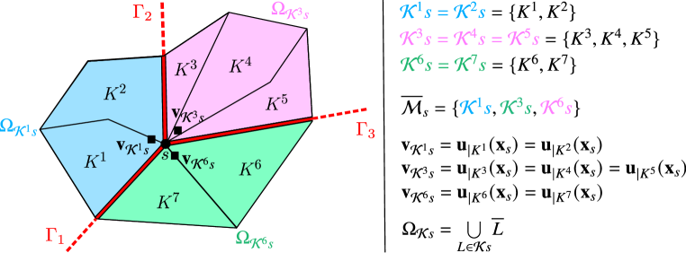
Figure 3: Degrees of freedom $\mathbf{v}_{\mathcal{K}s}$, ${\mathcal{K}s}\in\overline{\mathcal{M}}_{s}$ at a given node $s\in\mathcal{V}_{\Gamma}$ with three intersecting fractures. $\mathbf{v}_{\mathcal{K}s}$ corresponds to the nodal unknown at node s located on the side $K$ of the fractures. Here, $\mathbf{u}$ is a fictive continuous function that $\mathbf{v}$ could interpolate, and is used to give a clearer meaning to the degrees of freedom on each side of the fracture.

Remark 3.1 (Two-sided bubbles vs. one-sided bubbles).

It is also possible to define the vector space $\mathbf{U}_{\mathcal{D}}$ with a bubble unknown on both sides of each fracture face (two-sided bubbles), which amounts to replacing $\mathcal{F}_{\Gamma,K}^{+}$ by $\mathcal{F}_{\Gamma}\cap\mathcal{F}_{K}$ in its definition. This can lead to a better stabilisation of the Lagrange multiplier as exhibited in the numerical section in Figure 9 at the price of additional unknowns. Moreover, two-sided bubbles raises additional difficulties for the extension of the scheme to non-matching meshes at matrix fracture interfaces as opposed to the one-sided bubble case where the Lagrange multiplier and bubble discrete spaces can be both defined on the same side of the interface.

The unknowns $\mathbf{v}_{{\mathcal{K}s}}$ correspond to the nodal displacements (see Figure 3), while the $\mathbf{v}_{{K\!\sigma}}$ are the bubble unknowns on the "+" side of the fracture face $\sigma$ (see Figure 4) corresponding to a correction of the face mean value with respect to the linear nodal reconstruction $\Pi^{{K\!\sigma}}\mathbf{v}_{\mathcal{D}}$ defined here after in (8). This additional bubble unknown is needed to ensure the stability of the mixed variational formulation based on face-wise constant Lagrange-multiplier along the network $\Gamma$.

Let $\mathcal{C}^{0}(\Omega\setminus\overline{\Gamma})$ denote the space of continuous functions $f:\Omega\setminus\overline{\Gamma}\to\mathbb{R}$ with finite limits on $\partial\Omega$ and each side of $\Gamma$. We define two interpolators $\mathcal{I}_{\mathcal{V},\mathcal{D}}:\mathcal{C}^{0}(\Omega\setminus\overline{\Gamma})^{d}\to\mathbf{U}_{\mathcal{D}}$ and $\mathcal{I}_{\mathcal{D}}:\mathcal{C}^{0}(\Omega\setminus\overline{\Gamma})^{d}\to\mathbf{U}_{\mathcal{D}}$ onto $\mathbf{U}_{\mathcal{D}}$. The first one only interpolates on the vertices: for $\mathbf{v}\in\mathcal{C}^{0}(\Omega\setminus\overline{\Gamma})^{d}$, $\mathcal{I}_{\mathcal{V},\mathcal{D}}\mathbf{v}\in\mathbf{U}_{\mathcal{D}}$ is given by

$$\begin{array}[]{ll}(\mathcal{I}_{\mathcal{V},\mathcal{D}}\mathbf{v})_{{\mathcal{K}s}}=\mathbf{v}_{|_{K}}({\bf x}_{s})&\mbox{ for all }s\in\mathcal{V},\,{\mathcal{K}s}\in\overline{\mathcal{M}}_{s},\,K\in{\mathcal{K}s},\\ (\mathcal{I}_{\mathcal{V},\mathcal{D}}\mathbf{v})_{{K\!\sigma}}=0&\mbox{ for all }\sigma\in\mathcal{F}_{\Gamma,K}^{+},\,K\in\mathcal{M}.\end{array}$$

The second one keeps the interpolated vertex values, and provides face values that correct the trace of the function to take into account the vertex values: $\mathcal{I}_{\mathcal{D}}\mathbf{v}\in\mathbf{U}_{\mathcal{D}}$ is defined by

$$\begin{array}[]{ll}(\mathcal{I}_{\mathcal{D}}\mathbf{v})_{{\mathcal{K}s}}=\mathbf{v}_{|_{K}}({\bf x}_{s})&\mbox{ for all }s\in\mathcal{V},\,{\mathcal{K}s}\in\overline{\mathcal{M}}_{s},\,K\in{\mathcal{K}s},\\[5.0pt] (\mathcal{I}_{\mathcal{D}}\mathbf{v})_{{K\!\sigma}}=\displaystyle\frac{1}{|\sigma|}\int_{\sigma}(\gamma^{{K\!\sigma}}{\mathbf{v}}-\Pi^{{K\!\sigma}}(\mathcal{I}_{\mathcal{V},\mathcal{D}}\mathbf{v}))&\mbox{ for all }\sigma\in\mathcal{F}_{\Gamma,K}^{+},\,K\in\mathcal{M}.\end{array}$$

Here, $\Pi^{{K\!\sigma}}$ is the reconstructed face value defined by (8) below (we note that this reconstructed value only depends on the degrees of freedom on the vertices).

The vectorial Lagrange multiplier accounts for the surface traction $-{\mathbf{T}}^{+}$ approximation on $\Gamma$. Its discretisation is defined by the space $\mathbf{M}_{\mathcal{D}}$ of face-wise constant vectorial functions

$$\mathbf{M}_{\mathcal{D}}=\big{\{}{\bm{\lambda}}_{\mathcal{D}}\in L^{2}(\Gamma)^{d}~{}:~{}{\bm{\lambda}}_{\mathcal{D}}({\bf x})={\bm{\lambda}}_{\sigma}~{}\forall\sigma\in\mathcal{F}_{\Gamma},\forall~{}{\bf x}\in\sigma\big{\}}.$$

For ${\bm{\lambda}}_{\mathcal{D}}\in\mathbf{M}_{\mathcal{D}}$, let us define its normal and tangential components by

$$\lambda_{\mathcal{D},\mathbf{n}}({\bf x})=\lambda_{\sigma,\mathbf{n}}={\bm{\lambda}}_{\sigma}\cdot\mathbf{n}_{{K\!\sigma}}\,\,\mbox{ and }\,\,{\bm{\lambda}}_{\mathcal{D},{\bm{\tau}}}({\bf x})={\bm{\lambda}}_{\sigma,{\bm{\tau}}}={\bm{\lambda}}_{\sigma}-\lambda_{\sigma,\mathbf{n}}\mathbf{n}_{{K\!\sigma}},~{}\forall~{}{\bf x}\in\sigma=K|L,~{}\sigma\in\mathcal{F}_{\Gamma}.$$

For ${\bm{\lambda}}_{\mathcal{D}}\in\mathbf{M}_{\mathcal{D}}$ we define the discrete dual cone of admissible Lagrange multipliers as

$$\mathbf{C}_{\mathcal{D}}\left(\lambda_{\mathcal{D},\mathbf{n}}\right)=\big{\{}{\bm{\mu}}_{\mathcal{D}}=\left(\mu_{\mathcal{D},\mathbf{n}},{\bm{\mu}}_{\mathcal{D},{\bm{\tau}}}\right)\in\mathbf{M}_{\mathcal{D}}~{}:~{}\mu_{\mathcal{D},\mathbf{n}}\geq 0,~{}|{\bm{\mu}}_{\mathcal{D},{\bm{\tau}}}|\leq F\lambda_{\mathcal{D},\mathbf{n}}\big{\}}.$$

3.3.2 Reconstruction operators

For each face $\sigma\in\mathcal{F}_{K}$, $K\in\mathcal{M}$, we define the tangential gradient reconstruction operator based on the nodal unknowns:

$$\nabla^{{K\!\sigma}}:\mathbf{U}_{\mathcal{D}}\to\mathbb P^{\,0}(\sigma)^{d\times d}\mbox{ such that, for all $\mathbf{v}_{\mathcal{D}}\in\mathbf{U}_{\mathcal{D}}$,}$$

$$\nabla^{{K\!\sigma}}\mathbf{v}_{\mathcal{D}}=\frac{1}{|\sigma|}\sum_{e=s_{1}s_{2}\in\mathcal{E}_{\sigma}}|e|{\mathbf{v}_{{\mathcal{K}s}_{1}}+\mathbf{v}_{{\mathcal{K}s}_{2}}\over 2}\otimes\mathbf{n}_{{\sigma e}},$$

and the linear function reconstruction operator

$$\Pi^{{K\!\sigma}}:\mathbf{U}_{\mathcal{D}}\to\mathbb P^{1}(\sigma)^{d}\mbox{ such that, for all $\mathbf{v}_{\mathcal{D}}\in\mathbf{U}_{\mathcal{D}}$,}$$ (8)

$$\Pi^{{K\!\sigma}}\mathbf{v}_{\mathcal{D}}({\bf x})=\nabla^{{K\!\sigma}}\mathbf{v}_{\mathcal{D}}\left({\bf x}-\overline{{\bf x}}_{\sigma}\right)+\overline{\mathbf{v}}_{{K\!\sigma}}\qquad\forall{\bf x}\in\sigma,$$

with

$$\overline{\mathbf{v}}_{{K\!\sigma}}=\sum_{s\in\mathcal{V}_{\sigma}}\omega_{s}^{\sigma}\mathbf{v}_{{\mathcal{K}s}}~{}~{}\text{and}~{}~{}\overline{{\bf x}}_{\sigma}=\sum_{s\in\mathcal{V}_{\sigma}}\omega_{s}^{\sigma}{\bf x}_{s},$$ (9)

where $\omega_{s}^{\sigma}$ are weights associated to the center of mass of the face $\sigma$ (so that $\overline{{\bf x}}_{\sigma}$ is the center of mass of $\sigma$ and $\sum_{s\in\mathcal{V}_{\sigma}}\omega_{s}^{\sigma}=1$).

For each fracture face $\sigma\in\mathcal{F}_{\Gamma}$, $\sigma=K|L$ we introduce the displacement jump operator:

$$\llbracket\cdot\rrbracket_{\sigma}:\mathbf{U}_{\mathcal{D}}\to\mathbb P^{\,0}(\sigma)^{d}\mbox{ such that, for all $\mathbf{v}_{\mathcal{D}}\in\mathbf{U}_{\mathcal{D}}$,}$$

$$\llbracket\mathbf{v}_{\mathcal{D}}\rrbracket_{\sigma}=\frac{1}{|\sigma|}\int_{\sigma}\left(\Pi^{{K\!\sigma}}\mathbf{v}_{\mathcal{D}}-\Pi^{{L\!\sigma}}\mathbf{v}_{\mathcal{D}}\right){\rm d}\sigma+\mathbf{v}_{{K\!\sigma}},$$

as well as its normal and tangential components $\llbracket\cdot\rrbracket_{\sigma,\mathbf{n}}=\llbracket\cdot\rrbracket_{\sigma}\cdot\mathbf{n}_{{K\!\sigma}}$ and $\llbracket\cdot\rrbracket_{\sigma,{\bm{\tau}}}=\llbracket\cdot\rrbracket_{\sigma}-\llbracket\cdot\rrbracket_{\sigma,\mathbf{n}}\,\mathbf{n}_{{K\!\sigma}}$.

Remark 3.2 (Discrete jump).

It can easily be checked that, if $\mathbf{v}\in C^{0}(\overline{\Omega}\backslash\Gamma)^{d}$, then

$$\llbracket\mathcal{I}_{\mathcal{D}}\mathbf{v}\rrbracket_{\sigma}=\frac{1}{|\sigma|}\int_{\sigma}\left(\gamma^{{K\!\sigma}}\mathbf{v}-\Pi^{{L\!\sigma}}\mathcal{I}_{\mathcal{D}}\mathbf{v}\right),$$

showing that $\llbracket\mathcal{I}_{\mathcal{D}}\mathbf{v}\rrbracket_{\sigma}$ is an approximation of the (average of the exact) jump, using the exact trace of $\mathbf{v}$ on the positive side and an approximate trace on the negative side.

In case of two bubbles (see Remark 3.1), the jump is defined by

$$\llbracket\mathbf{v}_{\mathcal{D}}\rrbracket_{\sigma}=\frac{1}{|\sigma|}\int_{\sigma}\left(\Pi^{{K\!\sigma}}\mathbf{v}_{\mathcal{D}}-\Pi^{{L\!\sigma}}\mathbf{v}_{\mathcal{D}}\right){\rm d}\sigma+(\mathbf{v}_{K\!\sigma}-\mathbf{v}_{L\!\sigma}),$$

and, when applied to interpolate vectors, this jump provides the average of the exact continuous jump:

$$\llbracket\mathcal{I}_{\mathcal{D}}\mathbf{v}\rrbracket_{\sigma}=\frac{1}{|\sigma|}\int_{\sigma}\llbracket\mathbf{v}\rrbracket.$$

For each cell $K$, we define the gradient reconstruction operator

$$\nabla^{K}:\mathbf{U}_{\mathcal{D}}\to\mathbb P^{\,0}(\sigma)^{d\times d}\mbox{ such that, for all $\mathbf{v}_{\mathcal{D}}\in\mathbf{U}_{\mathcal{D}}$,}$$ (10)

$$\nabla^{K}\mathbf{v}_{\mathcal{D}}=\sum_{\sigma\in\mathcal{F}_{\Gamma,K}^{+}}\frac{|\sigma|}{|K|}\mathbf{v}_{{K\!\sigma}}\otimes\mathbf{n}_{{K\!\sigma}}+\sum_{\sigma\in\mathcal{F}_{K}}\frac{|\sigma|}{|K|}\overline{\mathbf{v}}_{{K\!\sigma}}\otimes\mathbf{n}_{K\!\sigma},$$

where $\overline{\mathbf{v}}_{K\!\sigma}$ is defined by (9). The linear function reconstruction operator is

$$\Pi^{K}:\mathbf{U}_{\mathcal{D}}\to\mathbb P^{1}(K)^{d}\mbox{ such that, for all $\mathbf{v}_{\mathcal{D}}\in\mathbf{U}_{\mathcal{D}}$,}$$ (11)

$$\Pi^{K}\mathbf{v}_{\mathcal{D}}({\bf x})=\nabla^{K}\mathbf{v}_{\mathcal{D}}\left({\bf x}-\overline{{\bf x}}_{K}\right)+\overline{\mathbf{v}}_{K}\quad\forall{\bf x}\in K,$$

with

$$\overline{\mathbf{v}}_{K}=\sum_{s\in\mathcal{V}_{K}}\omega_{s}^{K}\mathbf{v}_{{\mathcal{K}s}}~{}~{}\text{and}~{}~{}\overline{{\bf x}}_{K}=\sum_{s\in\mathcal{V}_{K}}\omega_{s}^{K}{\bf x}_{s}.$$

where $\omega_{s}^{K}$ are weights such that $\overline{{\bf x}}_{K}$ is the center of mass of $K$ and $\sum_{s\in\mathcal{V}_{K}}\omega_{s}^{K}=1$. Note that, by construction, all these local reconstruction operators are exact on linear functions in the sense that $\nabla^{K}\mathcal{I}_{\mathcal{D}}\mathbf{p}=\nabla\mathbf{p}$ and $\Pi^{K}\mathcal{I}_{\mathcal{D}}\mathbf{p}=\mathbf{p}$ for all $\mathbf{p}\in\mathbb P^{1}(K)^{d}$, and $\nabla^{K\!\sigma}\mathcal{I}_{\mathcal{D}}\mathbf{p}=\nabla_{\bm{\tau}}\mathbf{p}$ and $\Pi^{K\!\sigma}\mathcal{I}_{\mathcal{D}}\mathbf{p}=\mathbf{p}$, for all $\mathbf{p}\in\mathbb P^{1}(\sigma)^{d}$.

Let us now define the global discrete reconstruction $\Pi_{\mathcal{D}}:\mathbf{U}_{\mathcal{D}}\to L^{2}(\Omega)^{d}$ and the global discrete gradient $\nabla_{\mathcal{D}}:\mathbf{U}_{\mathcal{D}}\to L^{2}(\Omega)^{d\times d}$ such that

$$\Pi_{\mathcal{D}}\mathbf{v}_{\mathcal{D}}({\bf x})=\Pi^{K}\mathbf{v}_{\mathcal{D}}({\bf x})\quad\mbox{ and }\quad\nabla_{\mathcal{D}}\mathbf{v}_{\mathcal{D}}({\bf x})=\nabla^{K}\mathbf{v}_{\mathcal{D}}\quad\mbox{ for all }{\bf x}\in K,~{}K\in\mathcal{M}.$$

From the discrete gradient, we deduce the following definitions:

$$\bbespilon_{\mathcal{D}}(\cdot)=\frac{1}{2}(\nabla_{\mathcal{D}}(\cdot)+\prescript{t}{}{\nabla_{\mathcal{D}}}(\cdot)),~{}{\rm div}_{\mathcal{D}}(\cdot)=\text{Tr}\left(\bbespilon_{\mathcal{D}}(\cdot)\right)~{}\text{and}~{}\bbsigma_{\mathcal{D}}(\cdot)=2\mu\bbespilon_{\mathcal{D}}(\cdot)+\lambda{\rm div}_{\mathcal{D}}(\cdot)\mathbb{I}.$$

Finally, we define the discrete displacement jump operator

$$\llbracket\cdot\rrbracket_{\mathcal{D}}:\mathbf{U}_{\mathcal{D}}\to L^{2}(\Gamma)^{d}\mbox{ such that, for all $\mathbf{v}_{\mathcal{D}}\in\mathbf{U}_{\mathcal{D}}$,}$$

$$\llbracket\mathbf{v}_{\mathcal{D}}\rrbracket_{\mathcal{D}}({\bf x})=\llbracket\mathbf{v}_{\mathcal{D}}\rrbracket_{\sigma},~{}\forall~{}{\bf x}\in\sigma,~{}\sigma\in\mathcal{F}_{\Gamma},$$

as well as its normal and tangential components,

$$\llbracket\mathbf{v}_{\mathcal{D}}\rrbracket_{\mathcal{D},\mathbf{n}}=\llbracket\mathbf{v}_{\mathcal{D}}\rrbracket_{\mathcal{D}}\cdot\mathbf{n}^{+},\quad\llbracket\mathbf{v}_{\mathcal{D}}\rrbracket_{\mathcal{D},{\bm{\tau}}}=\llbracket\mathbf{v}_{\mathcal{D}}\rrbracket_{\mathcal{D}}-\llbracket\mathbf{v}_{\mathcal{D}}\rrbracket_{\mathcal{D},\mathbf{n}}\mathbf{n}^{+}.$$

The discrete $H^{1}$-like semi-norm on $\mathbf{U}_{\mathcal{D}}$ is defined by: for all $\mathbf{u}_{\mathcal{D}}\in{\bf x}_{\mathcal{D}}$,

$$\|\mathbf{u}_{\mathcal{D}}\|_{\mathcal{D}}:=\left(\sum_{K\in\mathcal{M}}\|\nabla^{K}\mathbf{u}_{\mathcal{D}}\|_{L^{2}(K)}^{2}+S_{K}(\mathbf{u}_{\mathcal{D}},\mathbf{u}_{\mathcal{D}})\right)^{1/2}$$

where the local stabilisation term is given by the bilinear form $S_{K}:\mathbf{U}_{\mathcal{D}}\times\mathbf{U}_{\mathcal{D}}\to\mathbb R$ such that, for all $\mathbf{u}_{\mathcal{D}},\mathbf{v}_{\mathcal{D}}\in\mathbf{U}_{\mathcal{D}}$,

$$S_{K}(\mathbf{u}_{\mathcal{D}},\mathbf{v}_{\mathcal{D}})=h_{K}^{d-2}\sum_{s\in\mathcal{V}_{K}}(\mathbf{u}_{{\mathcal{K}s}}-\Pi^{K}\mathbf{u}_{\mathcal{D}}({\bf x}_{s}))\cdot(\mathbf{v}_{{\mathcal{K}s}}-\Pi^{K}\mathbf{v}_{\mathcal{D}}({\bf x}_{s}))+\sum_{\sigma\in\mathcal{F}_{\Gamma,K}^{+}}h_{K}^{d-2}\,\mathbf{u}_{{K\!\sigma}}\cdot\mathbf{v}_{{K\!\sigma}}.$$ (12)

3.3.3 Discrete mixed variational formulation

We can now introduce the mixed variational discretisation of the contact-mechanical problem (6). Find $(\mathbf{u}_{\mathcal{D}}^{n},{\bm{\lambda}}_{\mathcal{D}}^{n})_{n=1,\ldots,N}\in(\mathbf{U}^{0}_{\mathcal{D}}\times\mathbf{C}_{\mathcal{D}}(\lambda_{\mathcal{D},\mathbf{n}}^{n}))^{N}$ such that, for all $(\mathbf{v}_{\mathcal{D}},{\bm{\mu}}_{\mathcal{D}})\in\mathbf{U}_{\mathcal{D}}\times\mathbf{C}_{\mathcal{D}}(\lambda_{\mathcal{D},\mathbf{n}}^{n})$ and $n=1,\cdots,N$, it holds

$$\int_{\Omega}\bbsigma_{\mathcal{D}}(\mathbf{u}_{\mathcal{D}}^{n}):\bbespilon_{\mathcal{D}}\left(\mathbf{v}_{\mathcal{D}}\right)+S_{\mu,\lambda,\mathcal{D}}\left(\mathbf{u}_{\mathcal{D}}^{n},\mathbf{v}_{\mathcal{D}}\right)-\int_{\Omega}b\Pi_{\mathcal{D}_{m}}p_{\mathcal{D}_{m}}^{n}{\rm div}_{\mathcal{D}}\mathbf{v}_{\mathcal{D}}$$

$$+\int_{\Gamma}\Pi_{\mathcal{D}_{f}}p_{\mathcal{D}_{f}}^{n}\llbracket\mathbf{v}_{\mathcal{D}}\rrbracket_{\mathcal{D},\mathbf{n}}+\int_{\Gamma}{\bm{\lambda}}_{\mathcal{D}}^{n}\cdot\llbracket\mathbf{v}_{\mathcal{D}}\rrbracket_{\mathcal{D}}=\sum_{K\in\mathcal{M}}\int_{K}\mathbf{f}_{K}^{n}\cdot\Pi_{\mathcal{D}}\mathbf{v}_{\mathcal{D}},$$ (13a)

$$\int_{\Gamma}\left((\mu_{\mathcal{D},\mathbf{n}}-\lambda_{\mathcal{D},\mathbf{n}}^{n})\llbracket\mathbf{u}_{\mathcal{D}}^{n}\rrbracket_{\mathcal{D},\mathbf{n}}+({\bm{\mu}}_{\mathcal{D},{\bm{\tau}}}-{\bm{\lambda}}_{\mathcal{D},{\bm{\tau}}}^{n})\cdot\llbracket\delta_{t}^{n}\mathbf{u}_{\mathcal{D}}\rrbracket_{\mathcal{D},{\bm{\tau}}}\right)\leq 0,$$ (13b)

with $\displaystyle\mathbf{f}_{K}^{n}=\frac{1}{|K|\Delta t^{n}}\int_{t^{n-1}}^{t^{n}}\int_{K}\mathbf{f}$, and where $S_{\mu,\lambda,\mathcal{D}}$ is the scaled stabilisation form defined by

$$S_{\mu,\lambda,\mathcal{D}}(\mathbf{u}_{\mathcal{D}},\mathbf{v}_{\mathcal{D}})=\sum_{K\in\mathcal{M}}(2\mu_{K}+\lambda_{K})S_{K}(\mathbf{u}_{\mathcal{D}},\mathbf{v}_{D}).$$

Thanks to the fracture face-wise constant Lagrange multiplier, the variational inequality (13b) together with ${\bm{\lambda}}_{\mathcal{D}}^{n}\in\mathbf{C}_{\mathcal{D}}(\lambda_{\mathcal{D},\mathbf{n}}^{n})$ can be equivalently replaced by the following non linear equations

$$\left\{\!\!\begin{array}[]{ll}&\lambda_{\mathcal{D},\mathbf{n}}^{n}=[\lambda_{\mathcal{D},\mathbf{n}}^{n}+\beta_{\mathcal{D},\mathbf{n}}\llbracket\mathbf{u}_{\mathcal{D}}^{n}\rrbracket_{\mathcal{D},\mathbf{n}}]_{\mathbb{R}^{+}}\\[2.15277pt] &\lambda_{\mathcal{D},{\bm{\tau}}}^{n}=[\lambda_{\mathcal{D},{\bm{\tau}}}^{n}+\beta_{\mathcal{D},{\bm{\tau}}}\llbracket\delta_{t}^{n}\mathbf{u}_{\mathcal{D}}\rrbracket_{\mathcal{D},{\bm{\tau}}}]_{F\lambda_{\mathcal{D},\mathbf{n}}^{n}},\end{array}\right.$$ (14)

where $\beta_{\mathcal{D},\mathbf{n}}>0$ and $\beta_{\mathcal{D},{\bm{\tau}}}>0$ are arbitrary given face-wise constant functions along $\Gamma$, $[x]_{\mathbb R^{+}}=\max\{0,x\}$, and $[\cdot]_{\alpha}$ is the projection on the ball of radius $\alpha$ centered at $0$, that is:

$$[{\bf x}]_{\alpha}=\left\{\begin{array}[]{ll}{\bf x}&\mbox{if }|{\bf x}|\leq\alpha,\\ \displaystyle\alpha{{\bf x}\over|{\bf x}|}&\mbox{otherwise}.\end{array}\right.$$

The equations (14) can be easily expressed locally to each fracture face and lead to an efficient semi-smooth Newton solver for the discrete contact-mechanics, see [3] for more details.

3.3.4 Discretisation of the coupling conditions

The set of equations (7)-(13a)-(14) is combined with the following coupling conditions:

$$\begin{array}[]{ll}&\delta_{t}^{n}\phi_{\mathcal{D}}=b~{}{\rm div}_{\mathcal{D}}\left(\delta_{t}^{n}\mathbf{u}_{\mathcal{D}}\right)+\frac{1}{M}\Pi_{\mathcal{D}_{m}}\delta_{t}^{n}p_{\mathcal{D}_{m}},\\[4.30554pt] &{\rm d}_{f,\mathcal{D}}^{n}={\rm d}_{f,\mathcal{D}}^{c}-\llbracket\mathbf{u}_{\mathcal{D}}^{n}\rrbracket_{\mathcal{D},\mathbf{n}},\end{array}$$ (15)

defining the discrete porosity $\phi_{\mathcal{D}}^{n}$ and fracture aperture ${\rm d}_{f,\mathcal{D}}^{n}$ for all $n\geq 0$, given a cell-wise constant approximation $\phi_{\mathcal{D}}^{0}$ of the initial porosity $\phi^{0}$ and a face-wise constant approximation ${\rm d}_{f,\mathcal{D}}^{c}$ of the contact aperture ${\rm d}_{f}^{c}$.

3.3.5 Discrete energy estimate

Proposition 3.3 (Discrete energy estimate).

Any solution $(p^{n}_{\mathcal{D}},\mathbf{u}^{n}_{\mathcal{D}},{\bm{\lambda}}_{D}^{n})_{n=1,\ldots,N}\in(X_{\mathcal{D}}^{0}\times\mathbf{U}^{0}_{\mathcal{D}}\times\mathbf{C}_{\mathcal{D}}(\lambda_{\mathcal{D},\mathbf{n}}^{n}))^{N}$ of the fully coupled scheme (7)-(13a)-(14)-(15) satisfies the following discrete energy estimates for all $n=1,\cdots,N$:

$$\delta_{t}^{n}\int_{\Omega}{1\over 2}\Bigl{(}\bbsigma_{\mathcal{D}}(\mathbf{u}_{\mathcal{D}}):\bbespilon_{\mathcal{D}}\left(\mathbf{u}_{\mathcal{D}}\right)+S_{\mu,\lambda,\mathcal{D}}\left(\mathbf{u}_{\mathcal{D}},\mathbf{u}_{\mathcal{D}}\right)+{1\over M}|\Pi_{\mathcal{D}_{m}}p_{\mathcal{D}_{m}}|^{2}\Bigr{)}+\int_{\Gamma}F\lambda_{\mathcal{D},\mathbf{n}}^{n}|\llbracket\delta_{t}^{n}\mathbf{u}_{\mathcal{D}}\rrbracket_{\mathcal{D},{\bm{\tau}}}|$$ (16)

$$+\int_{\Omega}\frac{\mathbb{K}_{m}}{\eta}\nabla_{\mathcal{D}_{m}}p_{\mathcal{D}_{m}}^{n}\cdot\nabla_{\mathcal{D}_{m}}p^{n}_{\mathcal{D}_{m}}+\int_{\Gamma}\frac{C_{f,\mathcal{D}}^{n-1}}{\eta}|\nabla_{\mathcal{D}_{f}}p_{\mathcal{D}_{f}}^{n}|^{2}+\sum_{\mathfrak{a}\in\{+,-\}}\int_{\Gamma}\Lambda_{f,\mathcal{D}}^{n-1}(\llbracket p_{\mathcal{D}}^{n}\rrbracket_{\mathcal{D}}^{\mathfrak{a}})^{2}$$

$$\leq\int_{\Omega}h_{m}\Pi_{\mathcal{D}_{m}}p^{n}_{\mathcal{D}_{m}}+\int_{\Gamma}h_{f}\nabla_{\mathcal{D}_{f}}p^{n}_{\mathcal{D}_{f}}+\sum_{K\in\mathcal{M}}\int_{K}\mathbf{f}_{K}^{n}\cdot\Pi_{\mathcal{D}}\delta_{t}^{n}\mathbf{u}_{\mathcal{D}}.$$

In addition, the discrete fracture aperture satisfies the lower bound ${\rm d}_{f,\mathcal{D}}^{n}\geq{\rm d}_{f,\mathcal{D}}^{c}$, which ensures the positivity of the fracture conductivity $C_{f,\mathcal{D}}^{n-1}$ and normal transmissivity $\Lambda_{f,\mathcal{D}}^{n-1}$.

Proof.

We only recall the main steps of the proof which follows the lines of the proof of [9, Eq. (19)]. We first recall, from e.g. [9, Lemma 4.1], that equations (14) equivalently state that

$$\lambda_{\mathcal{D},\mathbf{n}}^{n}\geq 0,\quad\llbracket\mathbf{u}_{\mathcal{D}}^{n}\rrbracket_{\mathcal{D},\mathbf{n}}\leq 0,\quad\lambda_{\mathcal{D},\mathbf{n}}^{n}\llbracket\mathbf{u}_{\mathcal{D}}^{n}\rrbracket_{\mathcal{D},\mathbf{n}}=0,$$

$$|\lambda_{\mathcal{D},{\bm{\tau}}}^{n}|\leq F\lambda_{\mathcal{D},\mathbf{n}}^{n},\quad\lambda_{\mathcal{D},{\bm{\tau}}}^{n}\cdot\llbracket\delta_{t}^{n}\mathbf{u}_{\mathcal{D}}\rrbracket_{\mathcal{D},{\bm{\tau}}}-F\lambda_{\mathcal{D},\mathbf{n}}^{n}|\llbracket\delta_{t}^{n}\mathbf{u}_{\mathcal{D}}\rrbracket_{\mathcal{D},{\bm{\tau}}}|=0.$$

We can deduce as in the proof of [9, Theorem 4.2] the following discrete persistency condition $\lambda_{\mathcal{D},\mathbf{n}}^{n}\llbracket\delta_{t}^{n}\mathbf{u}_{\mathcal{D}}\rrbracket_{\mathcal{D},\mathbf{n}}\geq 0$, from which results the following dissipative property of the contact term

$$\int_{\Gamma}{\bm{\lambda}}_{\mathcal{D}}^{n}\cdot\llbracket\delta_{t}^{n}\mathbf{u}_{\mathcal{D}}\rrbracket_{\mathcal{D}}\geq\int_{\Gamma}F\lambda_{\mathcal{D},\mathbf{n}}^{n}|\llbracket\delta_{t}^{n}\mathbf{u}_{\mathcal{D}}\rrbracket_{\mathcal{D},{\bm{\tau}}}|\geq 0.$$

Then, setting $\mathbf{v}_{\mathcal{D}}=\delta_{t}^{n}\mathbf{u}_{\mathcal{D}}$ in (13a) and $q_{\mathcal{D}_{m}}=p^{n}_{\mathcal{D}_{m}}$ in (7), taking into account the coupling equations (15) and the discrete dissipative property of the contact term, we obtain (16). The lower bound on the discrete fracture aperture follows directly from (15) and $\llbracket\mathbf{u}_{\mathcal{D}}^{n}\rrbracket_{\mathcal{D},\mathbf{n}}\leq 0$. ∎

Following [9], in order to deduce from (16) a priori estimates and the existence of a discrete solution, we need to establish a discrete Korn inequality in $\mathbf{U}^{0}_{\mathcal{D}}$ and a discrete inf-sup condition for the bilinear form $\int_{\Gamma}{\bm{\lambda}}_{\mathcal{D}}\cdot\llbracket\mathbf{v}_{\mathcal{D}}\rrbracket_{\mathcal{D}}$ in $\mathbf{U}^{0}_{\mathcal{D}}\times\mathbf{M}_{\mathcal{D}}$. This is a work in progress which requires new developments related to the additional bubble unknowns and to fracture networks including tips and intersections.

3.4 An equivalent VEM formulation of the contact-mechanics

We show here that the previous discretisation of the mechanics has an equivalent VEM formulation based on the same displacement degrees of freedom leading to a $\mathbb P^{1}$-bubble VEM discretisation. The VEM framework provides an extension of Finite Element Methods (FEM) to polyhedral meshes. As for FEM, it builds a subspace $\mathbf{V}_{h}$ of $\mathbf{U}$ by gluing the local spaces $\mathbf{V}_{h}^{K}\subset H^{1}(K)^{d}$ defined in each cell $K\in\mathcal{M}$. On the other hand, the basis functions cannot be computed analytically and a projector $\pi^{K}$ from $\mathbf{V}_{h}^{K}$ onto $\mathbb P^{1}(K)^{d}$ is defined such that it is computable on $\mathbf{V}_{h}^{K}$ and preserves the consistency. The bilinear form is then obtained from the continuous one using the projector and by stabilising its kernel. In the following, we first exhibit the connection between the VEM face $\pi^{{K\!\sigma}}$ and cell $\pi^{K}$ projectors and the previous reconstruction operators respectively $\Pi^{K\sigma}$ and $\Pi^{K}$. Then, the VEM local and global spaces are defined leading to the stabilised bilinear form and the equivalent VEM mixed variational formulation of the contact-mechanical problem. The unisolvence of the degrees of freedom in the VEM space $\mathbf{V}_{h}$ is also shown. Detailed proofs are reported in Appendix A.

3.4.1 VEM projectors, function spaces and equivalent mixed variational formulation

For each $K\in\mathcal{M}$, let $\pi^{K}$ be the local projection operator defined by:

$$\pi^{K}:\mathcal{C}^{0}(\overline{K})^{d}\to\mathbb P^{1}(K)^{d}\mbox{ such that, for all $\mathbf{v}\in\mathcal{C}^{0}(\overline{K})^{d}$},$$ (17)

$$\pi^{K}\mathbf{v}=\Pi^{K}\circ\mathcal{I}_{\mathcal{D}}\mathbf{v},$$

where, by abuse of notation, the interpolator $\mathcal{I}_{\mathcal{D}}$ is applied to the extension by zero of $\mathbf{v}$ outside $\overline{K}$. Similarly, for each $\sigma\in\mathcal{F}_{K}$, $K\in\mathcal{M}$, let $\pi^{{K\!\sigma}}$ be the local projection operator defined by:

$$\pi^{{K\!\sigma}}:\mathcal{C}^{0}(\overline{\sigma})^{d}\to\mathbb P^{1}(\sigma)^{d}\mbox{ such that, for all $\mathbf{v}\in\mathcal{C}^{0}(\overline{\sigma})^{d}$},$$ (18)

$$\pi^{{K\!\sigma}}\mathbf{v}=\Pi^{{K\!\sigma}}\circ\mathcal{I}_{\mathcal{D}}\mathbf{v}.$$

We can now introduce the VEM local space for the displacement field on each cell $K\in\mathcal{M}$:

$$\begin{split}\mathbf{V}_{h}^{K}=\Big{\{}\mathbf{v}\in\mathcal{C}^{0}(\overline{K})^{d}|~{}&\gamma^{{K\!\sigma}}{\mathbf{v}}\in\mathbf{V}_{h}^{{K\!\sigma}},~{}\forall~{}\sigma\in\mathcal{F}_{K};\\ &\Delta\mathbf{v}\in\mathbb P^{1}(K)^{d};~{}\int_{K}(\pi^{K}\mathbf{v})\cdot\mathbf{p}=\int_{K}\mathbf{v}\cdot\mathbf{p},~{}\forall~{}\mathbf{p}\in\mathbb P^{1}(K)^{d}\Big{\}},\end{split}$$ (19)

with

$$\begin{split}\mathbf{V}_{h}^{{K\!\sigma}}=\Big{\{}\mathbf{v}\in\mathcal{C}^{0}(\overline{\sigma})^{d}|~{}&\gamma^{\sigma_{e}}{\mathbf{v}}\in\mathbb P^{1}(e)^{d},~{}\forall~{}e\in\mathcal{E}_{\sigma};\\ &\Delta_{{\bm{\tau}}}\mathbf{v}\in\mathbb P^{1}(\sigma)^{d}~{}\text{in}~{}\sigma;~{}\int_{\sigma}(\pi^{{K\!\sigma}}\mathbf{v})\cdot\mathbf{p}=\int_{\sigma}\mathbf{v}\cdot\mathbf{p},~{}\forall~{}\mathbf{p}\in(\mathbb Q_{{K\!\sigma}})^{d}\Big{\}},\end{split}$$ (20)

where $\mathbb Q_{K\!\sigma}=\mathbb P^{1}(\sigma)$ if $\sigma\in\mathcal{F}_{K}\setminus\mathcal{F}_{\Gamma,K}^{+}$ – corresponding to the no bubble case – and $\mathbb Q_{K\!\sigma}$ is a complementary space of constant functions in $\mathbb P^{1}(\sigma)$ if $\sigma\in\mathcal{F}_{\Gamma,K}^{+}$ – corresponding to the bubble case.

Lemma 3.4 (Link between discrete reconstructions and elliptic projectors).

For all $K\in\mathcal{M}$, the projector $\pi^{K}:\mathbf{V}_{h}^{K}\to\mathbb P^{1}(K)^{d}$ is the elliptic projector, that is, it satisfies: for all $\mathbf{v}\in\mathbf{V}_{h}^{K}$,

$$\int_{K}\nabla(\pi^{K}\mathbf{v}):\nabla\mathbf{q}=\int_{K}\nabla\mathbf{v}:\nabla\mathbf{q}\qquad\forall~{}\mathbf{q}\in\mathbb P^{1}(K)^{d},$$ (21a)

$$(\pi^{K}\mathbf{v})(\overline{{\bf x}}_{K})=\sum_{s\in\mathcal{V}_{K}}\omega_{s}^{K}\mathbf{v}({\bf x}_{s}).$$ (21b)

For all $\sigma\in\mathcal{F}_{K}$, the projector $\pi^{K\!\sigma}:\mathbf{V}_{h}^{K\!\sigma}\to\mathbb P^{1}(\sigma)^{d}$ is the elliptic projector for the tangential gradient, that is, it satisfies: for all $\mathbf{v}\in\mathbf{V}_{h}^{K\!\sigma}$,

$$\int_{\sigma}\nabla_{{\bm{\tau}}}(\pi^{{K\!\sigma}}\mathbf{v}):\nabla_{{\bm{\tau}}}\mathbf{q}=\int_{\sigma}\nabla_{{\bm{\tau}}}\mathbf{v}:\nabla_{{\bm{\tau}}}\mathbf{q}\qquad\forall~{}\mathbf{q}\in\mathbb P^{1}(\sigma)^{d},$$ (22a)

$$(\pi^{{K\!\sigma}}\mathbf{v})(\overline{{\bf x}}_{\sigma})=\sum_{s\in\mathcal{V}_{\sigma}}\omega_{s}^{\sigma}\mathbf{v}({\bf x}_{s}).$$ (22b)

Proof.

See Appendix A.1. ∎

As a consequence of (21) and the fact that $\bbsigma$ has constant coefficients on each cell, we have, for all $K\in\mathcal{M}$ and $\mathbf{v}\in\mathbf{V}_{h}^{K}$,

$$\int_{K}\bbsigma(\pi^{K}\mathbf{v}):\bbespilon(\mathbf{q})=\int_{K}\bbsigma(\mathbf{v}):\bbespilon(\mathbf{q})\qquad\forall~{}\mathbf{q}\in\mathbb P^{1}(K)^{d}$$ (23)

For $\mathbf{v}\in\mathbf{V}^{K}_{h}$, the VEM local degrees of freedom are the same as in the previous setting, namely the nodal value $\mathbf{v}_{{\mathcal{K}s}}=\mathbf{v}({\bf x}_{s})=(\mathcal{I}_{\mathcal{D}}\mathbf{v})_{\mathcal{K}s}$ at each node $s\in\mathcal{V}_{K}$ and the bubble value $\mathbf{v}_{K\!\sigma}=(\mathcal{I}_{\mathcal{D}}\mathbf{v})_{{K\!\sigma}}$ for each $\sigma\in\mathcal{F}_{\Gamma,K}^{+}$ (see Figure 4). Note that the bubble unknown can also be expressed using the local projector $\pi^{{K\!\sigma}}$ as follows:

$$\mathbf{v}_{K\!\sigma}=(\mathcal{I}_{\mathcal{D}}\mathbf{v})_{{K\!\sigma}}=\frac{1}{|\sigma|}\int_{\sigma}\Bigl{(}\gamma^{{K\!\sigma}}{\mathbf{v}}-\pi^{{K\!\sigma}}({\gamma^{{K\!\sigma}}\mathbf{v}})\Bigr{)}.$$

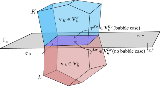
Figure 4: $\mathbb P^{1}$-bubble VEM

The global VEM space for the displacement field is obtained as usual by glueing the local VEM spaces in a conforming way in $H^{1}(\Omega\setminus\overline{\Gamma})^{d}$. It is defined by

$$\begin{split}\mathbf{V}_{h}=\Big{\{}\mathbf{v}\in H^{1}(\Omega\setminus\overline{\Gamma})^{d}\cap\,\mathcal{C}^{0}(\Omega\setminus\overline{\Gamma})^{d}|~{}\mathbf{v}_{|_{K}}\in\mathbf{V}_{h}^{K},~{}\forall K\in\mathcal{M}\Big{\}},\end{split}$$

and we denote by $\mathbf{V}_{h}^{0}$ its subspace with vanishing values on the boundary $\partial\Omega$. Note that the vector of all degrees of freedom of $\mathbf{v}\in\mathbf{V}_{h}$ is precisely $\mathcal{I}_{\mathcal{D}}\mathbf{v}\in\mathbf{U}_{\mathcal{D}}$. We define $\pi^{h}$ as the global projection operator onto the broken polynomial space $\mathbb{P}^{1}(\mathcal{M})^{d}$, such that, $\forall\mathbf{v}\in\mathbf{V}_{h}$, $(\pi^{h}\mathbf{v})_{|K}=\pi^{K}({\mathbf{v}}_{|K})$. The diagram (24) illustrates the fondamental relation between $\pi^{h}$ and $\Pi_{\mathcal{D}}$.

(24)

The mixed variational formulation for the contact-mechanical problem in the $\mathbb P^{1}$-bubble VEM framework is defined by: find $(\mathbf{u}^{n},{\bm{\lambda}}_{\mathcal{D}}^{n})\in\mathbf{V}_{h}^{0}\times\mathbf{C}_{\mathcal{D}}(\lambda_{\mathcal{D},\mathbf{n}}^{n})$, $n=1,\cdots,N$ such that

$$\displaystyle\sum_{K\in\mathcal{M}}\int_{K}\bbsigma(\pi^{K}\mathbf{u}^{n}):\bbespilon(\pi^{K}\mathbf{v})+S_{\mu,\lambda,\mathcal{D}}(\mathcal{I}_{\mathcal{D}}\mathbf{u}^{n},\mathcal{I}_{\mathcal{D}}\mathbf{v})-\sum_{K\in\mathcal{M}}\int_{K}b\Pi_{\mathcal{D}_{m}}p_{\mathcal{D}_{m}}^{n}{\rm div}(\pi^{K}\mathbf{v})$$

$$+\sum_{\sigma\in\mathcal{F}_{\Gamma}}\int_{\sigma}\Pi_{\mathcal{D}_{f}}p_{\mathcal{D}_{f}}^{n}\llbracket\mathbf{v}\rrbracket_{\mathbf{n}}+\sum_{\sigma\in\mathcal{F}_{\Gamma}}\int_{\sigma}{\bm{\lambda}}_{\mathcal{D}}^{n}\cdot\llbracket\mathbf{v}\rrbracket=\sum_{K\in\mathcal{M}}\int_{K}\mathbf{f}^{n}_{K}\cdot\pi^{K}\mathbf{v},$$ (25a)

$$\sum_{\sigma\in\mathcal{F}_{\Gamma}}\int_{\sigma}\Bigl{(}(\mu_{\mathcal{D},\mathbf{n}}-\lambda_{\mathcal{D},\mathbf{n}}^{n})\llbracket\mathbf{u}^{n}\rrbracket_{\mathbf{n}}+({\bm{\mu}}_{\mathcal{D},{\bm{\tau}}}-{\bm{\lambda}}_{\mathcal{D},{\bm{\tau}}}^{n})\cdot\llbracket\delta_{t}^{n}\mathbf{u}\rrbracket_{{\bm{\tau}}}\Bigr{)}\leq 0,$$ (25b)

for all $(\mathbf{v},{\bm{\mu}}_{\mathcal{D}})\in\mathbf{V}_{h}^{0}\times\mathbf{C}_{\mathcal{D}}(\lambda_{\mathcal{D},\mathbf{n}}^{n})$ and $n=1,\cdots,N$.

It is straightforward to observe that the variational formulation (25) is equivalent to (13) based on the correspondence $\mathbf{u}_{\mathcal{D}}=\mathcal{I}_{\mathcal{D}}\mathbf{u}$ and $\mathbf{v}_{\mathcal{D}}=\mathcal{I}_{\mathcal{D}}\mathbf{v}$. The term $\int_{\sigma}\llbracket\mathbf{u}\rrbracket{\rm d}\sigma$ is computable as we have, for $\sigma=K|L$,

$$\int_{\sigma}\llbracket\mathbf{u}\rrbracket{\rm d}\sigma=\int_{\sigma}\Bigl{(}\pi^{{K\!\sigma}}(\gamma^{{K\!\sigma}}\mathbf{u})-\pi^{{L\!\sigma}}(\gamma^{{L\!\sigma}}\mathbf{u})\Bigr{)}+|\sigma|(\mathcal{I}_{\mathcal{D}}\mathbf{u})_{{K\!\sigma}},$$

since $\int_{\sigma}\gamma^{L\!\sigma}\mathbf{u}=\int_{\sigma}\pi^{L\!\sigma}(\gamma^{L\!\sigma}\mathbf{u})$ by the condition in (20) for $\mathbf{V}_{h}^{L\!\sigma}$ applied with $\mathbf{p}$ constant (which is valid since $L$ is not a bubble side of $\sigma$). The stabilisation term $S_{\mu,\lambda,\mathcal{D}}(\mathcal{I}_{\mathcal{D}}\mathbf{u}^{n},\mathcal{I}_{\mathcal{D}}\mathbf{v})$ matches the classical VEM "dofi-dofi" approach [17] based on the degrees of freedom (see Appendix A.2 for a detailed proof). The consistency of the local bilinear form

$$a_{\mathcal{D}}^{K}(\mathbf{u},\mathbf{v})=\displaystyle\int_{K}\bbsigma(\pi^{K}\mathbf{u}):\bbespilon(\pi^{K}\mathbf{v})+(2\mu_{K}+\lambda_{K})S_{K}(\mathbf{u}_{\mathcal{D}},\mathbf{v}_{D})$$

derives from (23) and the fact that $\pi^{K}\mathbf{w}=\mathbf{w}$ for all $\mathbf{w}\in\mathbb P^{1}(K)^{d}$. The stability of the discretisation relying on a discrete Korn inequality and a discrete inf-sup condition involves technical difficulties related to the additional bubble unknown and to the fracture network. It will be presented in a future work. In this paper, our primary emphasis is on the definition of the scheme and its numerical assessment.

3.4.2 Degrees of freedom unisolvence

Proposition 3.5.

For all $K\in\mathcal{M}$, the local degrees of freedom associated to $K$ are unisolvent for $\mathbf{V}_{h}^{K}$. As a consequence, the degrees of freedom of $\mathbf{U}_{\mathcal{D}}$ are unisolvent for $\mathbf{V}_{h}$.

Proof.

Let us consider a mesh element $K$ that includes at least a fracture face (the case without any fracture face being done similarly and in a simpler way). Let us show that the local interpolation operator ${\mathcal{I}_{\mathcal{D}}}_{|{\mathbf{V}_{h}^{K}}}:\mathbf{V}_{h}^{K}\to\mathbf{U}_{\mathcal{D}}$ that extracts the degrees of freedom from a given function of $\mathbf{V}_{h}^{K}$ is injective. We thus want to show that any function $\mathbf{v}\in\mathbf{V}_{h}^{K}$ such that:

$$(\mathcal{I}_{\mathcal{D}}\mathbf{v})_{{\mathcal{K}s}}=0,\,\forall~{}s\in\mathcal{V}_{K},$$ (26a)

$$(\mathcal{I}_{\mathcal{D}}\mathbf{v})_{{K\!\sigma}}=0,\,\forall~{}\sigma\in\mathcal{F}_{\Gamma,K}^{+},$$ (26b)

is identically zero in $K$. From (26a), we get that $\gamma^{{K\!\sigma}}\mathbf{v}=0$ on $\partial\sigma$, for all $\sigma\in\mathcal{F}_{K}$. In order to show that $\gamma^{{K\!\sigma}}\mathbf{v}=0$ on $\sigma$, it suffices to show that

$$\int_{\sigma}(\gamma^{{K\!\sigma}}\mathbf{v})\cdot\mathbf{p}=0,\forall~{}\mathbf{p}\in\mathbb P^{1}(\sigma)^{d}.$$ (27)

Indeed, suppose that (27) is satisfied, then one can write

$$0\underbrace{=}_{\Delta_{{\bm{\tau}}}\gamma^{{K\!\sigma}}\mathbf{v}\in\mathbb P^{1}(\sigma)^{d}}\int_{\sigma}(\gamma^{{K\!\sigma}}\mathbf{v})\cdot\Delta_{{\bm{\tau}}}\gamma^{{K\!\sigma}}\mathbf{v}\underbrace{=}_{\gamma^{{K\!\sigma}}\mathbf{v}\,=\,0~{}\text{on}~{}\partial\sigma}\int_{\sigma}\nabla_{{\bm{\tau}}}\gamma^{{K\!\sigma}}\mathbf{v}\cdot\nabla_{{\bm{\tau}}}\gamma^{{K\!\sigma}}\mathbf{v},$$

which directly implies $\gamma^{{K\!\sigma}}\mathbf{v}=0$ on $\sigma$ since $\gamma^{{K\!\sigma}}\mathbf{v}=0$ on $\partial\sigma$. By the condition in (20), we have, for all $\mathbf{p}\in(\mathbb Q_{K\!\sigma})^{d}$,

$$\int_{\sigma}(\gamma^{{K\!\sigma}}\mathbf{v})\cdot\mathbf{p}=\int_{\sigma}\pi^{{K\!\sigma}}(\gamma^{{K\!\sigma}}\mathbf{v})\cdot\mathbf{p}=0,$$ (28)

where the conclusion follows from (26a) which implies $\pi^{{K\!\sigma}}(\gamma^{{K\!\sigma}}\mathbf{v})=0$. If $\sigma\not\in\mathcal{F}_{\Gamma,K}^{+}$ then $\mathbb Q_{K\!\sigma}=\mathbb P^{1}(\sigma)$ and (27) follows. Otherwise, still using $\pi^{{K\!\sigma}}(\gamma^{{K\!\sigma}}\mathbf{v})=0$ we have

$$\frac{1}{|\sigma|}\int_{\sigma}\gamma^{{K\!\sigma}}{\mathbf{v}}=\int_{\sigma}(\gamma^{{K\!\sigma}}{\mathbf{v}}-\pi^{{K\!\sigma}}(\gamma^{{K\!\sigma}}\mathbf{v}))=(\mathcal{I}_{\mathcal{D}}\mathbf{v})_{{K\!\sigma}}=0,$$

the conclusion following from (26b). Combined with (28) which is valid for any $\mathbf{p}$ in a complement space of $\mathbb P^{0}(\sigma)$, this proves that (27) also holds. It results that $\mathbf{v}=0$ on $\partial K$. We repeat a similar (but simpler, since the condition in (19) is already expressed against test functions in $\mathbb P^{1}(K)^{d}$) procedure on $K$, to finally obtain $\mathbf{v}=0$ on $K$. Therefore, ${\mathcal{I}_{\mathcal{D}}}_{|{\mathbf{V}_{h}^{K}}}$ is injective. Proceeding as in [1], it is easy to show that $\text{dim}(\mathbf{V}_{h}^{K})\geq d\cdot(\#\mathcal{V}_{K}+\#\mathcal{F}_{\Gamma,K}^{+})$ which implies that $\mathcal{I}_{\mathcal{D}}$ defines a bijection from $\mathbf{V}_{h}^{K}$ to the vector space $(\mathbb R^{d})^{\#\mathcal{V}_{K}+\#\mathcal{F}_{\Gamma,K}^{+}}$ of degrees of freedom of the cell $K$. Consequently, the degrees of freedom in $K$ are unisolvent for $\mathbf{V}_{h}^{K}$ for all $K\in\mathcal{M}$. ∎

4 Numerical experiments

The objective of this section is to assess the numerical convergence of the discretisation of the poromechanical model with frictional contact at matrix fracture interfaces defined by (7)-(13a)-(14)-(15). We first investigate in Section 4.1 the discretisation of the contact-mechanics on the stand alone static contact-mechanical model. Then, we consider in Section 4.2 the discretisation of the fully coupled poromechanical model.

In the following test cases, the Lamé coefficients can be defined from the Young modulus $E$ and the Poisson coefficient $\nu$ by $\mu=\frac{E}{2(1+\nu)}$ and $\lambda=\frac{\nu E}{(1+\nu)(1-2\nu)}$. The 2D test cases presented in this section are performed with the 3D code using 3D meshes obtained by extrusion in the $z$ direction of the 2D meshes of the $(x,y)$ domain, with one layer of cells of thickness $1$. The $z$ components of the displacement field and of the Lagrange multiplier are set to zero and homogeneous Neumann boundary conditions are imposed at $z=0$ and $z=1$ boundaries. The resulting discretisation is equivalent to the 2D version of the scheme.

4.1 Stand alone static contact-mechanics

The numerical convergence of the mixed $\mathbb P^{1}$-bubble VEM–$\mathbb P^{0}$ discretisation (13a)-(14) is investigated on three static contact-mechanical test cases obtained from (2)-(3)-(4) by setting the matrix $p_{m}$ and fracture $p_{f}$ pressures to zero and replacing $\llbracket\partial_{t}\mathbf{u}\rrbracket_{\bm{\tau}}$ by $\llbracket\mathbf{u}\rrbracket_{\bm{\tau}}$ in the contact term. The first one consider a manufactured 3D analytical solution with a single non-immersed fracture and a frictionless contact model. The second test case is based on an analytical solution for a single fracture in contact slip state immersed in an unbounded 2D domain. The last test case compares our discretisation to a Nitsche $\mathbb P^{1}$ Finite Element Method (FEM) on a 2D domain with 6 fractures.

4.1.1 3D manufactured solution for a frictionless static contact-mechanical model

We consider the 3D domain $\Omega=(-1,1)^{3}$ with the single non-immersed fracture $\Gamma=\{0\}\times(-1,1)^{2}$. The friction coefficient $F$ is set to zero corresponding to a frictionless contact and the Lamé coefficients are set to $\mu=\lambda=1$. The exact solution

$$\mathbf{u}(x,y,z)=\left\{\hskip 5.69046pt\begin{array}[]{lll}\left({\begin{array}[]{c}g(x,y)p(z)\\ p(z)\\ x^{2}p(z)\\ \end{array}}\right)&\mbox{ if }z\geq 0,\\[4.30554pt] \left({\begin{array}[]{c}h(x)p^{+}(z)\\ h(x)\left(p^{+}(z)\right)^{\prime}\\ -\int_{0}^{x}h(\xi){\rm d}\xi\left(p^{+}(z)\right)^{\prime}\\ \end{array}}\right)&\mbox{ if }z<0,~{}x\ <0,\\[4.30554pt] \left({\begin{array}[]{c}h(x)p^{-}(z)\\ h(x)\left(p^{-}(z)\right)^{\prime}\\ -\int_{0}^{x}h(\xi){\rm d}\xi\left(p^{-}(z)\right)^{\prime}\\ \end{array}}\right)&\mbox{ if }z<0,~{}x\ \geq 0,\end{array}\right.$$

with $g(x,y)=-\sin(\frac{\pi x}{2})\cos(\frac{\pi y}{2})$, $p(z)=z^{2}$, $h(x)=\cos(\frac{\pi x}{2})$, $p^{+}(z)=z^{4}$ and $p^{-}(z)=2z^{4}$, is designed to satisfy the frictionless contact conditions at the matrix fracture interface $\Gamma$. The right hand side $\mathbf{f}=-{\rm div}\bbsigma(\mathbf{u})$ is deduced and the trace of $\mathbf{u}$ is imposed as Dirichlet boundary condition on $\partial\Omega$. Note that the fracture $\Gamma$ is in contact state for $z>0$ ($\llbracket\mathbf{u}\rrbracket_{\mathbf{n}}=0$) and open for $z<0$ with the normal jump $\llbracket\mathbf{u}\rrbracket_{\mathbf{n}}=-\min(z,0)^{4}$ depending only on $z$. The convergence of the mixed $\mathbb P^{1}$-bubble VEM–$\mathbb P^{0}$ formulation is investigated on families of uniform Cartesian, tetrahedral and hexahedral meshes. Starting from a uniform Cartesian mesh, the hexahedral mesh is generated by random perturbation of the nodes and by cutting the faces into two triangles (see Figure 5).

Figure 5: Example of randomly perturbated Cartesian cell with non planar faces cut into two triangles

Figure 6 exhibits the relative $L^{2}$ norms of the errors $\mathbf{u}-\Pi_{\mathcal{D}}\mathbf{u}_{\mathcal{D}}$, $\llbracket\mathbf{u}\rrbracket-\llbracket\mathbf{u}_{\mathcal{D}}\rrbracket_{\mathcal{D}}$, $\nabla{\mathbf{u}}-\nabla_{\mathcal{D}}\mathbf{u}_{\mathcal{D}}$ and $\lambda_{\mathbf{n}}-\lambda_{\mathcal{D},\mathbf{n}}$ on the three family of refined meshes as a function of the cubic root of the number of cells. It shows, as expected for such a smooth solution, a second-order convergence for $\mathbf{u}$ and $\llbracket\mathbf{u}\rrbracket$ with all families of meshes. A first-order convergence is obtained for $\nabla{\mathbf{u}}$ and $\lambda_{\mathbf{n}}$ with both the hexahedral and tetrahedral families of meshes, while a second order super convergence is observed with the family of Cartesian meshes.

Figure 6: Relative $L^{2}$ norms of the errors $\mathbf{u}-\Pi_{\mathcal{D}}\mathbf{u}_{\mathcal{D}}$, $\llbracket\mathbf{u}\rrbracket-\llbracket\mathbf{u}_{\mathcal{D}}\rrbracket_{\mathcal{D}}$, $\nabla{\mathbf{u}}-\nabla_{\mathcal{D}}\mathbf{u}_{\mathcal{D}}$ and $\lambda_{\mathbf{n}}-\lambda_{\mathcal{D},\mathbf{n}}$ as a function of the square root of the number of cells, using the families of Cartesian (a), tetrahedral (b) and hexahedral (c) meshes. Test case of Section 4.1.1.

Figure 7 plots, for the hexahedral family of meshes, the face-wise constant normal jump $\llbracket\mathbf{u}_{\mathcal{D}}\rrbracket_{\mathcal{D},\mathbf{n}}$ on $\Gamma$ as well as the nodal normal jumps as a function of $z$ along the “broken” line corresponding to $x=y=0$ before perturbation of the mesh. We recall that the continuous normal jump depends only on $z$.

Figure 7: (a) Face-wise constant normal jump $\llbracket\mathbf{u}_{\mathcal{D}}\rrbracket_{\mathcal{D},\mathbf{n}}$ on $\Gamma$ obtained on the hexahedral mesh with $2^{3m}$ cells, $m=5$. (b) Nodal normal jumps along the line $x=y=0$ as a function of $z$ both for the discrete solutions on the hexahedral meshes with $2^{3m}$ cells, $m=3,4,5$ and for the continuous solution depending only on $z$. Test case of Section 4.1.1.

4.1.2 Unbounded 2D domain with a single fracture under compression

This test case presented in [35, 25, 26] consists of a 2D unbounded domain containing a single fracture and subject to a compressive remote stress $\sigma$ = 100 MPa. The fracture inclination with respect to the $x$-direction is $\psi=\pi/9$, its length is $2\ell=2$ m, and the friction coefficient is $F=1/\~{A}\'{E}3$. Young’s modulus and Poisson’s ratio are set to $E=25$ GPa and $\nu=0.25$. The analytical solution in terms of the Lagrange multiplier $\lambda_{\mathbf{n}}$ and of the jump of the tangential displacement field is given by:

$$\lambda_{\mathbf{n}}=\sigma\sin^{2}(\psi),\quad|{\llbracket\mathbf{u}\rrbracket}_{{\bm{\tau}}}|=\frac{4(1-\nu)}{E}\sigma\sin(\psi)\left(\cos(\psi)-F\sin(\psi)\right)\sqrt{\ell^{2}-(\ell^{2}-\tau^{2})},$$ (29)

where $0\leq\tau\leq 2\ell$ is a curvilinear abscissa along the fracture. Note that since $\lambda_{\mathbf{n}}>0$, we have $\llbracket\mathbf{u}\rrbracket_{\mathbf{n}}=0$ on the fracture. Boundary conditions are imposed on $\mathbf{u}$ at specific nodes of the mesh, as shown in Figure 8, to respect the symmetry of the expected solution. For this simulation, we sample a $320\text{m}\times 320\,\rm m$ square, and carry out uniform refinements at each step in such a way to compute the solution on meshes containing 100, 200, 400, and 800 faces on the fracture (corresponding, respectively, to 12 468, 49 872, 199 488, and 797 952 triangular elements). The initial mesh is refined in a neighborhood of the fracture; starting from this mesh, we perform global uniform refinements at each step.

Figure 9 shows the comparison between the analytical and numerical Lagrange multipliers $\lambda_{\mathbf{n}}$ and tangential displacement jump $\llbracket\mathbf{u}\rrbracket_{{\bm{\tau}}}$ computed on the finest mesh with either one-sided or two-sided bubbles along the fracture (see Remark 3.1). The Lagrange multiplier $\lambda_{\mathbf{n}}$ presents some oscillations in a neighborhood of the fracture tips. As already explained in [25], this is due to the sliding of faces close to the fracture tips (in this test case, all fracture faces are in a contact-slip state). As could be expected, the two-sided bubble case significantly reduces the Lagrange multiplier oscillations compared with the one-sided bubble case, due to a better stabilisation (but at the cost of more degrees of freedom). In both cases, the discrete tangential displacement jump cannot be distinguished from the analytical solution on this fine mesh. Figure 10 and Table 1 display, for the one-sided bubble case, the convergence of the tangential displacement jump and of the normal Lagrange multiplier as a function of the size of the largest fracture face denoted by $h$. Note that the $L^{2}$ error for the Lagrange multiplier is computed $5\%$ away from each tip to circumvemt the lack of convergence induced by the oscillations as in [25]. A first-order convergence for the displacement jump and a $1.5$ convergence order for the Lagrange multiplier are observed. The former (low) rate is related to the low regularity of $\llbracket\mathbf{u}\rrbracket_{\bm{\tau}}$ close to the tips (cf. the analytical expression (29)), the latter (higher than expected) rate is likely related to the fact that $\lambda_{\mathbf{n}}$ is constant. Table 1 also shows the robust convergence of the semi-smooth Newton algorithm on the family of refined meshes.

(a)

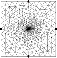
(b)

Figure 8: Unbounded domain containing a single fracture under uniform compression (a) and mesh including nodes for boundary conditions ($\blacklozenge$: $u_{x}=0$, $\blacksquare$: $u_{y}=0$), for the example of Section 4.1.2.

Figure 9: Comparison between the numerical and analytical solutions on the finest mesh (with 800 fracture faces), in terms of $\lambda_{\mathbf{n}}$ with one-sided bubbles (a) and two-sided bubbles (b), example of Section 4.1.2.

Figure 10: Convergence of the relative $L^{2}$ error of $\llbracket\mathbf{u}\rrbracket_{\bm{\tau}}-\llbracket\mathbf{u}_{\mathcal{D}}\rrbracket_{\mathcal{D},{\bm{\tau}}}$ and of $\lambda_{\mathbf{n}}-\lambda_{\mathcal{D},\mathbf{n}}$ away from the tip, as a function of the size of the largest fracture face denoted by $h$, one-sided bubble case. Test case of Section 4.1.2.

$\#\mathcal{F}_{\Gamma}$	$N^{\text{dof}}$	$E_{L^{2}}^{\llbracket\mathbf{u}\rrbracket_{{\bm{\tau}}}}$	order $\llbracket\mathbf{u}\rrbracket_{{\bm{\tau}}}$	$E_{L^{2}}^{\lambda_{\mathbf{n}}}$	order $\lambda_{\mathbf{n}}$	$N^{\text{Newton}}$
100	13028	4.36E-2	-	2.23E-2	-	2
200	50992	1.80E-2	1.27	8.84E-3	1.34	2
400	201728	7.71E-3	1.25	2.91E-3	1.60	2
800	802432	3.46E-3	1.15	9.89E-4	1.56	2

Table 1: Relative $L^{2}$ errors and convergence orders for $\llbracket\mathbf{u}\rrbracket_{\bm{\tau}}-\llbracket\mathbf{u}_{\mathcal{D}}\rrbracket_{\mathcal{D},{\bm{\tau}}}$ and $\lambda_{\mathbf{n}}-\lambda_{\mathcal{D},\mathbf{n}}$ away from the tip, and number $N^{\text{Newton}}$ of semi-smooth Newton iterations for the different meshes with $N^{\text{dof}}$ scalar degrees of freedom (3D mesh) and $\#\mathcal{F}_{\Gamma}$ fracture faces. One-sided bubble case. Test case of Section 4.1.2.

4.1.3 2D Discrete Fracture Matrix model with 6 fractures: static contact-mechanics test case

To illustrate the behavior of our approach on a more complex fracture network, we consider the Discrete Fracture Matrix (DFM) model test case presented in [6, Section 4.1], where a $2\text{m}\times 1\text{m}\times 1\text{m}$ domain including a network $\Gamma=\bigcup_{i=1}^{6}\Gamma_{i}$ of fractures is considered, see Figure 11. Fracture 1 is made up of two sub-fractures forming a corner, whereas one of the tips of fracture 5 lies on the boundary of the domain. We use the same values of Young’s modulus and Poisson’s ratio, $E=4$ GPa and $\nu=0.2$, and the same set of boundary conditions as in [6], that is, the two left and right sides of the domain are free, and we impose $\mathbf{u}=0$ on the lower side and $\mathbf{u}=\prescript{t}{}{[}0.005\,\text{m},-0.002\,\text{m}]$ on the top side. The friction coefficient is $F_{i}({\bf x})=0.5(1+10\cdot e^{-D_{i}^{2}({\bf x})/0.005})$, with $i\in\{1,...,6\}$ the fracture index, ${\bf x}\in\Gamma_{i}$ a generic point on fracture $i$ and $D_{i}({\bf x})$ the minimum distance from ${\bf x}$ to the tips of fracture $i$ (the bend in fracture 1 is not considered as a tip).

Since no closed-form solution is available for this test case, to evaluate the convergence of our method we compute a reference solution on a fine mesh made of 730 880 mesh element. Figure 12 shows the convergence rates obtained for both $\llbracket\mathbf{u}\rrbracket$ and $\bm{\lambda}$. Analogously to the previous example, we perform uniform mesh refinements at each step, and do not refine only in a neighborhood of tips. As in [6], an asymptotic first-order convergence is observed for the vector Lagrange multiplier for all fractures, except fracture 4 which exhibits a convergence rate close to 2 owing to its entire contact-stick state, and fracture 1 which exhibits a lower rate due to the additional singularity induced by the corner. For the jump of the displacement field across fractures, we obtain an asymptotic convergence rate equal to 1.5 for all fractures. In Figure 13, we compare the error curves of the displacement jump $\llbracket\mathbf{u}\rrbracket$ and the traction mean value $\left({\mathbf{T}}^{\scriptstyle{+}}-{\mathbf{T}}^{-}\right)/2$ between our method and the Nitsche $\mathbb P^{1}$ FEM for contact-mechanics [3], for fractures 1, 2, and 3. It is noticeable that we have approximately the same convergence for both methods. Taking advantage of the flexibility of the polytopal VEM method, we consider a modified mesh obtained by inserting a node at the midpoint of each fracture-edge generating 4 nodes triangles on both sides of the fractures. Figure 14 exhibits the tangential displacement jumps obtained with the original coarse mesh and the one refined only along the fractures with these 4 nodes triangles. We observe that the refined mesh solution better captures the stick-slip transition than the one on the original mesh. This improvement is achieved with a minor computational overcost, as the volumetric discretization remains unchanged, and we exclusively refine along the fractures.

Figure 11: 3D prism / 2D Rectangular domain with six fractures. Fracture 1 comprises two sub-fractures making a corner, and fracture 5 has a tip on the boundary. The contact state of each fracture obtained by the simulation is also shown on the same mesh: Mixed $\mathbb P^{1}$-bubble VEM–$\mathbb P^{0}$ (left) vs. Nitsche $\mathbb P^{1}$ FEM (right). Test case of section 4.1.3.

Figure 12: Relative $L_{2}$ error between the current and reference solutions in terms of $\llbracket\mathbf{u}\rrbracket$ and ${\bm{\lambda}}$ as a function of the size of the largest fracture face, yielding a 1.5-order of convergence for $\llbracket\mathbf{u}\rrbracket$ and 1st order of convergence for ${\bm{\lambda}}$. Test case of section 4.1.3.

Figure 13: Relative $L_{2}$ error, as a function of the size of the largest fracture face, between the current and reference solutions in terms of $\left({\mathbf{T}}^{\scriptstyle{+}}-{\mathbf{T}}^{-}\right)/2$ (top) and $\llbracket\mathbf{u}\rrbracket$ (bottom) along fractures 1,2 and 3 from left to right: Mixed $\mathbb P^{1}$-bubble VEM–$\mathbb P^{0}$ vs. Nitsche $\mathbb P^{1}$ FEM. Test case of section 4.1.3.

Figure 14: Tangential jumps $\llbracket\mathbf{u}\rrbracket_{{\bm{\tau}}}$ on fracture 1 (left) and fracture 3 (right) obtained on the original coarse triangular mesh "tri3 mesh” and the refined mesh only along the fractures using 4 nodes triangles "tri3-tri4 mesh". Test case of section 4.1.3.

4.2 Poromechanical test cases

The objective here is first to compare our discretisation with the one presented in [3] combining a Nitsche $\mathbb P^{2}$ FEM for the contact-mechanics with the HFV scheme for the flow on triangular 2D meshes. The second objective is to assess the robustness of our approach on a 3D test case with a fracture network including intersections. The coupled nonlinear system is solved at each time step of the simulation using the fixed-stress algorithm [32] adapted to mixed-dimensional models following [28]. At each fixed stress iteration, the Darcy linear problem at given fracture aperture and porosity is solved using a GMRes iterative solver preconditioned by AMG, and the contact-mechanical model at given pressures $(p_{m},p_{f})$ is solved using the semi-smooth Newton method combined with a direct sparse linear solver.

4.2.1 2D DFM with 6 fractures: poromechanical test case

This test case presented in [3, Section 5] basically adds the fluid flow to the contact-mechanical test case of Section 4.1.3. On the mechanical side, the only changes are related to the friction coefficient fixed here to $F=0.5$ and to the following time dependent Dirichlet boundary conditions

$$\mathbf{u}(t,{\bf x})=\left\{\hskip 5.69046pt\begin{array}[]{ll}\displaystyle\prescript{t}{}{[}0.005\,\text{m},-0.002\,\text{m}]\frac{4t}{T}\,~{}~{}~{}~{}~{}~{}\text{if}~{}t\leq\frac{T}{4},\\[4.30554pt] \prescript{t}{}{[}0.005\,\text{m},-0.002\,\text{m}]\,~{}~{}~{}~{}~{}~{}~{}~{}~{}~{}\text{otherwise}\end{array}\right.$$

on the top boundary. Concerning the flow boundary conditions, all sides are assumed impervious, except the left one, on which a pressure equal to the initial pressure $10^{5}$ Pa is prescribed. To fully exploit the capabilities of the HFV flow discretization, we consider the following anisotropic permeability tensor in the matrix:

$$\mathbb{K}_{m}=K_{m}\left(\begin{array}[]{cc}1&0\\ 0&1/2\end{array}\right).$$

The permeability coefficient is set to $K_{m}=10^{-15}$ m², the Biot coefficient to $b=0.5$, the Biot modulus to $M=10$ GPa, the dynamic viscosity to $\eta=10^{-3}$ Pa${\cdot}$s. For further details related to the Darcy flow, we refer the reader to [3, Section 5]. The triangular meshes are the same as in Section 4.1.3, the final time is set to $T=2000\,\text{s}$, and a uniform time stepping with 20 time steps is used for the Euler implicit time integration. Figure 15 exhibits the good convergence behavior of the mean matrix pressure as a function of time on a family of three uniformly refined meshes, in comparison to a numerical reference solution obtained on a finer mesh using the Nitsche $\mathbb P^{2}$ FEM presented in [3] and the same Euler implicit time integration with the same time stepping. The matrix over-pressure (w.r.t. the initial pressure) obtained at final time with our discretisation is also compared in Figure 16 to the one obtained by the Nitsche $\mathbb P^{2}$ FEM of [3] on the same mesh using the same time integration. Notably, we found that the numerical results of the two methods are very similar, with almost no noticeable differences. Figure 17 shows the mean fracture aperture and pressure as functions of time for the family of three uniformly refined meshes, showing a good spatial convergence to the numerical reference solution. Note that the fracture pressure basically matches the traces of the matrix pressure due to the high conductivity of the fractures. Figure 18 exhibits a 1.5-order convergence rate of the discrete $l^{2}$ errors in time of the matrix mean pressure and porosity and the fracture mean pressure, aperture and tangential jump, using the fine mesh Nitsche $\mathbb P^{2}$ FEM solution as reference.

Figure 15: Mean pressure in the matrix as a function of time for a family of three uniformly refined meshes in comparison to the numerical reference solution obtained on a finer mesh using the Nitsche $\mathbb P^{2}$ FEM presented in [3]. Test case of Section 4.2.1.

Figure 16: Matrix over-pressures (w.r.t. the initial pressure) in Pa at final time obtained with the mixed $\mathbb P^{1}$-bubble VEM–$\mathbb P^{0}$/HFV scheme (left) vs. the Nitsche $\mathbb P^{2}$ FEM/HFV scheme (right) on the same mesh with the same time integration. Test case of Section 4.2.1.

Figure 17: Mean fracture aperture and pressure as functions of time for a family of three uniformly refined meshes in comparison to the numerical reference solution obtained on a finer mesh using the Nitsche $\mathbb P^{2}$ FEM presented in [3]. Test case of Section 4.2.1.

Figure 18: Relative discrete $l^{2}$ error in time, as a function of the size of the largest fracture face denoted by $h$, between the numerical and reference solutions for the mean matrix pressure and porosity (left), and the mean fracture pressure, aperture, and tangential jump $\llbracket\mathbf{u}\rrbracket_{{\bm{\tau}}}$ (right). Test case of Section 4.2.1.

4.2.2 3D DFM with intersecting fractures

The objective of this test case is to assess the ability of the discretisation and of the nonlinear solver to simulate a poromechanical test case on a 3D DFM with intersecting fractures. We consider the domain $\Omega=(0,1\,\mbox{\rm m})^{3}$ with the fracture network $\Gamma$ illustrated in Figure 19 discretised by a tetrahedral mesh consisting of either $47$k or $127$k cells.

The Young’s modulus and Poisson’s ratio are set to $E=4\,\mathrm{GPa}$ and $\nu=0.2$, and the friction coefficient to $F=0.5$. The Biot coefficient is set to $b=0.5$ and the Biot modulus to $M=10\,\mathrm{GPa}$. Dirichlet boundary conditions are imposed on the bottom and top boundaries for the displacement field with $\mathbf{u}=0$ on the bottom boundary $z=0$ and the following time dependent displacement on the top boundary $z=1$

$$\mathbf{u}(t,x,y,1)=\left\{\hskip 5.69046pt\begin{array}[]{ll}\displaystyle\prescript{t}{}{[}0.002\,\text{m},0.002\,\text{m},-0.002\,\text{m}]\frac{2t}{T}\,~{}~{}~{}~{}~{}~{}\text{if}~{}t\leq\frac{T}{2},\\[4.30554pt] \prescript{t}{}{[}0.002\,\text{m},0.002\,\text{m},-0.002\,\text{m}]\,~{}~{}~{}~{}~{}~{}~{}~{}~{}~{}\text{otherwise},\end{array}\right.$$

for $(x,y)\in(0,1)^{2}$. Homogeneous Neumann boundary conditions are set on the lateral sides for the mechanics. Regarding the Darcy flow, the matrix permeability tensor is set to $\mathbb{K}_{m}=K_{m}\mathbb{I}$ with $K_{m}=10^{-14}\mathrm{~{}m}^{2}$, and the dynamic viscosity to $\eta=10^{-3}\mathrm{~{}Pa}\cdot\mathrm{s}$. The initial matrix porosity is set to $\phi_{m}^{0}=0.2$ and the fracture aperture corresponding to both contact state and zero displacement field is given by $\text{d}_{f}^{c}=10^{-3}\,\mathrm{m}$. The initial pressure in the matrix and fracture network is $p_{m}^{0}=p_{f}^{0}=10^{5}\mathrm{~{}Pa}$. Notice that the initial fracture aperture differs from $\text{d}_{f}^{c}$, since it is computed by solving the contact-mechanics given the initial pressures $p_{m}^{0}$ and $p_{f}^{0}$. The final time is set to $T=20\mathrm{~{}s}$ and the time integration uses a uniform time stepping with $20$ time steps. The boundary conditions for the flow are impervious except at the lateral boundaries $y=0$ and $y=1$ where a fixed pressure $p_{m}=10^{5}\mathrm{~{}Pa}$ is prescribed.

Figure 20 and Figure 21 exhibits respectively the normal and the ${\bm{\tau}}_{2}$ tangential component of the displacement jump along the fractures at final time $t=T$, obtained on the $127$k and the $47$k cells meshes. Note that $(\mathbf{n},{\bm{\tau}}_{1},{\bm{\tau}}_{2})$ is a coordinate system local to each fracture. It illustrates qualitatively the convergence of the displacement jump along the fracture when the mesh is refined.

Figure 22 plots the cumulated total number of semi-smooth Newton iterations for the contact-mechanical model as a function of time both for the one-sided and two-sides bubble cases and for both mesh sizes with 47k and 127k cells. It illustrates the robustness of the nonlinear solver with respect to the mesh size and the (moderate) benefit of the stronger stabilisation obtained with the two-sided bubble case.

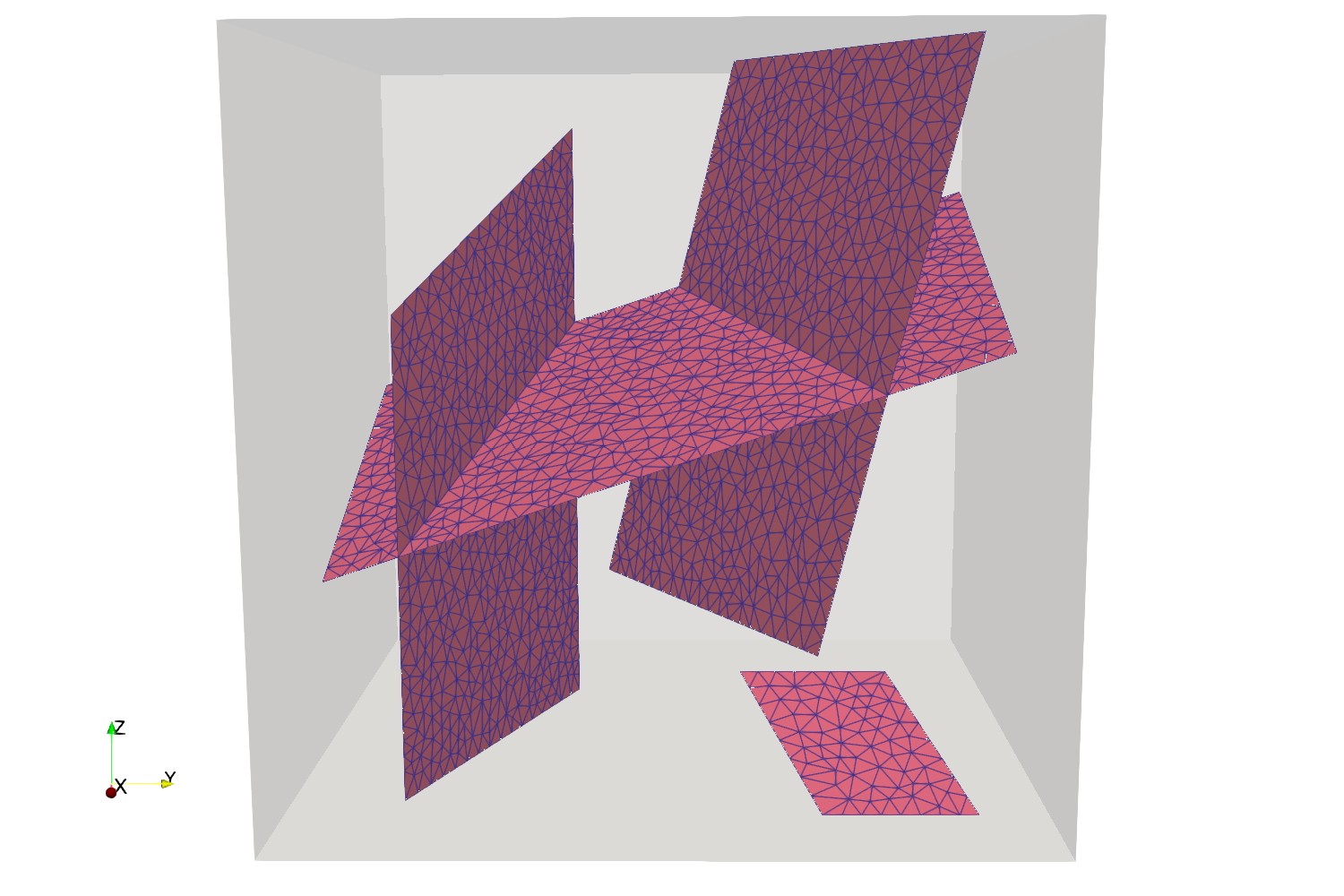
Figure 19: Tetrahedral mesh of the 3D DFM with intersecting fractures comprising roughly $127$k cells. Test case of Section 4.2.2.

Figure 20: Normal jump with the $47$k cells mesh (left) and the $127$k cells mesh (right), obtained at final time $t=T$. Test case of section 4.2.2.

Figure 21: The ${\bm{\tau}}_{2}$ component of the tangential jump with the $47$k cells mesh (left) and the $127$k cells mesh (right), obtained at final time $t=T$. Test case of section 4.2.2.

Figure 22: Total number of semi-smooth Newton iterations for the contact-mechanical model as a function of time, with both one-sided and two-sided bubbles and for both meshes with $47$k cells (left) and $127$k cells (right). Test case of Section 4.2.2.

5 Conclusions

We have developped in this work a novel numerical scheme for contact-mechanics in fractured/faulted porous media. It is based on a mixed formulation, using face-wise constant approximations of the Lagrange multipliers and a polytopal scheme for the displacement with fully discrete spaces and reconstruction operators. This scheme is applicable on meshes with generic elements, and employs a bubble degree of freedom to ensure the inf–sup stability with the Lagrange multiplier space. It was shown that this fully discrete scheme is equivalent to a low-order bubble-VEM scheme, which is to our knowledge the first of its kind. The numerical scheme has been validated on several 2D and 3D test cases both for the stand alone contact-mechanical and the fully coupled mixed-dimensional poromechanical models.

The stability and convergence analysis of this mixed $\mathbb P^{1}$ VEM-bubble–$\mathbb P^{0}$ discretisation of the contact-mechanics requires new developments related to the additional bubble unknowns and to fracture networks including tips and intersections. This is a work in progress that will establish the discrete Korn inequality and the inf–sup condition.

Appendix A Analysis of the elliptic projectors and stabilisation in the VEM space

A.1 Proof of Lemma 3.4

For $K\in\mathcal{M}$ and $\sigma\in\mathcal{F}_{K}$, let us show that the local projectors $\pi^{K}$ and $\pi^{{K\!\sigma}}$ defined in (17) and (18), respectively, satisfy conditions (21) and (22) in $\mathbf{V}_{h}^{K}$.

For $\mathbf{v}\in\mathbf{V}_{h}^{K}$, one can write:

$$\int_{K}\nabla\mathbf{v}={} \sum_{\sigma\in\mathcal{F}_{K}}\int_{\sigma}\gamma^{{K\!\sigma}}\mathbf{v}\otimes\mathbf{n}_{{K\!\sigma}}$$

$$={} \sum_{\sigma\in\mathcal{F}_{\Gamma,K}^{+}}\int_{\sigma}\gamma^{{K\!\sigma}}\mathbf{v}\otimes\mathbf{n}_{{K\!\sigma}}+\frac{1}{|K|}\sum_{\sigma\in\mathcal{F}_{K}\setminus\mathcal{F}_{\Gamma,K}^{+}}\int_{\sigma}\gamma^{{K\!\sigma}}\mathbf{v}\otimes\mathbf{n}_{{K\!\sigma}}$$

$$={} \sum_{\sigma\in\mathcal{F}_{\Gamma,K}^{+}}\left[\int_{\sigma}\Bigl{(}\gamma^{{K\!\sigma}}\mathbf{v}-\pi^{{K\!\sigma}}(\gamma^{{K\!\sigma}}\mathbf{v})\Bigr{)}\otimes\mathbf{n}_{{K\!\sigma}}\right]+\sum_{\sigma\in\mathcal{F}_{K}}\int_{\sigma}\pi^{{K\!\sigma}}(\gamma^{{K\!\sigma}}\mathbf{v})\otimes\mathbf{n}_{{K\!\sigma}},$$

where we have used the Stokes formula in the first equality and, in the conclusion, subtracted and added

$$\sum_{\sigma\in\mathcal{F}_{\Gamma,K}^{+}}\int_{\sigma}\pi^{{K\!\sigma}}(\gamma^{{K\!\sigma}}\mathbf{v})\otimes\mathbf{n}_{{K\!\sigma}}$$

and used the relation $\int_{\sigma}\gamma^{{K\!\sigma}}\mathbf{v}=\int_{\sigma}\pi^{{K\!\sigma}}(\gamma^{{K\!\sigma}}\mathbf{v})$ for all $\sigma\in\mathcal{F}_{K}\setminus\mathcal{F}_{\Gamma,K}^{+}$ (see the integral condition in (20)). We therefore have

$$\int_{K}\nabla\mathbf{v}=\sum_{\sigma\in\mathcal{F}_{\Gamma,K}^{+}}|\sigma|(\mathcal{I}_{\mathcal{D}}\mathbf{v})_{{K\!\sigma}}\otimes\mathbf{n}_{{K\!\sigma}}+\sum_{\sigma\in\mathcal{F}_{K}}\int_{\sigma}\pi^{{K\!\sigma}}(\gamma^{{K\!\sigma}}\mathbf{v})\otimes\mathbf{n}_{{K\!\sigma}}$$ (30)

The relation (18) between $\pi^{K\!\sigma}$ and $\Pi^{K\!\sigma}$ and the definition (8) of $\Pi^{K\!\sigma}$ (recalling that $\int_{\sigma}({\bf x}-\overline{{\bf x}}_{\sigma})=0$) yield

$$\int_{\sigma}\pi^{{K\!\sigma}}(\gamma^{{K\!\sigma}}\mathbf{v})=\int_{\sigma}\Pi^{{K\!\sigma}}(\mathcal{I}_{\mathcal{D}}\gamma^{{K\!\sigma}}\mathbf{v})=|\sigma|\overline{(\mathcal{I}_{\mathcal{D}}\gamma^{{K\!\sigma}}\mathbf{v})}_{K\!\sigma}=|\sigma|\overline{(\mathcal{I}_{\mathcal{D}}\mathbf{v})}_{K\!\sigma}$$

(where $\overline{(\mathcal{I}_{\mathcal{D}}\mathbf{v})}_{K\!\sigma}$ is defined by (9) with $\mathcal{I}_{\mathcal{D}}\mathbf{v}$ instead of $\mathbf{v}$). Hence, (30) and the definition (10) of $\nabla^{K}=\nabla\Pi^{K}$ show that

$$\int_{K}\nabla\mathbf{v}=|K|\nabla^{K}(\mathcal{I}_{\mathcal{D}}\mathbf{v})=\int_{K}\nabla\Pi^{K}(\mathcal{I}_{\mathcal{D}}\mathbf{v})=\int_{K}\nabla\pi^{K}\mathbf{v}.$$

Taking $\mathbf{q}\in\mathbb P^{1}(K)^{d}$ and multiplying this relation with $\nabla\mathbf{q}$ (which is constant) yields (21a).

To get the relation (21b), on the other hand, we use , the fact that $\pi^{K}\mathbf{v}=\Pi^{K}\mathcal{I}_{\mathcal{D}}\mathbf{v}$ is linear and (11) to write

$$(\pi^{K}\mathbf{v})(\overline{{\bf x}}_{K})=\frac{1}{|K|}\int_{K}\Pi^{K}\mathcal{I}_{\mathcal{D}}\mathbf{v}=\overline{(\mathcal{I}_{\mathcal{D}}\mathbf{v})}_{K}=\sum_{s\in\mathcal{V}_{K}}\omega_{s}^{K}(\mathcal{I}_{\mathcal{D}}\mathbf{v})_{{\mathcal{K}s}}=\sum_{s\in\mathcal{V}_{K}}\omega_{s}^{K}\mathbf{v}({\bf x}_{s}).$$

We now turn to (22). If $\mathbf{v}\in\mathbf{V}_{h}^{K\!\sigma}$, then $\mathbf{v}\in\mathbb P^{1}(e)$ on each edge $e$ of $\sigma$ and thus, by Stokes formula,

$$\int_{\sigma}\nabla_{{\bm{\tau}}}\mathbf{v}=\sum_{e\in\mathcal{E}_{\sigma}}\int_{e}\gamma^{\sigma_{e}}\mathbf{v}\otimes\mathbf{n}_{{\sigma e}}=\sum_{e=s_{1}s_{2}\in\mathcal{E}_{\sigma}}|e|{(\mathcal{I}_{\mathcal{D}}\mathbf{v})_{K_{s_{1}}}+(\mathcal{I}_{\mathcal{D}}\mathbf{v})_{K_{s_{2}}}\over 2}\otimes\mathbf{n}_{{\sigma e}}=|\sigma|\nabla^{{K\!\sigma}}(\mathcal{I}_{\mathcal{D}}\mathbf{v}).$$

The conclusion of (22) then follows as above.

A.2 Discrete stability term $S_{\mu,\lambda,\mathcal{D}}$ as a VEM dofi-dofi stabilisation

Given $\mathbf{u},\mathbf{v}\in\mathbf{V}^{K}_{h}$, let us set $\mathbf{u}_{\mathcal{D}}=\mathcal{I}_{\mathcal{D}}\mathbf{u}$, $\mathbf{v}_{\mathcal{D}}=\mathcal{I}_{\mathcal{D}}\mathbf{v}$. The usual dofi-dofi approach first introduces the bilinear form based on the VEM degrees of freedom

$$s_{K}(\mathbf{u},\mathbf{v})=h^{d-2}_{K}\Bigl{(}\sum_{s\in\mathcal{V}_{K}}\mathbf{u}_{{\mathcal{K}s}}\mathbf{v}_{{\mathcal{K}s}}+\sum_{\sigma\in\mathcal{F}_{\Gamma,K}^{+}}\mathbf{u}_{K\!\sigma}\mathbf{v}_{K\!\sigma}\Bigr{)},$$

and defines the stabilisation bilinear form as

$$\mathcal{S}_{K}(\mathbf{u},\mathbf{v})=s_{K}(\mathbf{u}-\pi^{K}\mathbf{u},\mathbf{v}-\pi^{K}\mathbf{v}).$$

The fact that $\mathcal{S}_{K}(\mathbf{u},\mathbf{v})=S_{K}(\mathcal{I}_{\mathcal{D}}\mathbf{u},\mathcal{I}_{\mathcal{D}}\mathbf{v})$ directly follows from the definition of $S_{K}$ in (12) and from the identities $(\mathbf{w}-\pi^{K}\mathbf{w})_{\mathcal{K}s}=(\mathcal{I}_{\mathcal{D}}\mathbf{w})_{\mathcal{K}s}-(\Pi^{K}\mathcal{I}_{\mathcal{D}}\mathbf{w})({\bf x}_{s})$ and $(\mathbf{w}-\pi^{K}\mathbf{w})_{K\!\sigma}=(\mathcal{I}_{\mathcal{D}}\mathbf{w})_{K\!\sigma}-(\mathcal{I}_{\mathcal{D}}\pi^{K}\mathbf{w})_{K\!\sigma}=(\mathcal{I}_{\mathcal{D}}\mathbf{w})_{K\!\sigma}$ for all $\mathbf{w}\in\mathbf{V}^{K}_{h}$ (we have used $(\mathcal{I}_{\mathcal{D}}\mathbf{q})_{{K\!\sigma}}=0$ whenever $\mathbf{q}\in\mathbb P^{1}(K)$, which follows from the fact that $\Pi^{K\!\sigma}(\mathcal{I}_{\mathcal{D}}\mathbf{q})=\mathbf{q}$ since $\mathbf{q}$ is linear).

References

• [1] Bashir Ahmad, Ahmed Alsaedi, Franco Brezzi, L Donatella Marini, and Alessandro Russo. Equivalent projectors for virtual element methods. Computers & Mathematics with Applications, 66(3):376–391, 2013.
• [2] Odd Andersen, Halvor M. Nilsen, and Xavier Raynaud. Virtual element method for geomechanical simulations of reservoir models. Computational Geosciences, 21(5):877–893, 2017.
• [3] Laurence Beaude, Franz Chouly, Mohamed Laaziri, and Roland Masson. Mixed and Nitsche’s discretizations of coulomb frictional contact-mechanics for mixed dimensional poromechanical models. Computer Methods in Applied Mechanics and Engineering, 413:116124, 2023.
• [4] L. Beirão Da Veiga, F. Brezzi, and L.D. Marini. Virtual elements for linear elasticity problems. SIAM Journal on Numerical Analysis, 51:794–812, 2013.
• [5] F. Ben Belgacem and Y. Renard. Hybrid finite element methods for the signorini problem. Mathematics of Computation, 72:1117–1145, 2003.
• [6] R. L. Berge, I. Berre, E. Keilegavlen, J. M. Nordbotten, and B. Wohlmuth. Finite volume discretization for poroelastic media with fractures modeled by contact mechanics. International Journal for Numerical Methods in Engineering, 121:644–663, 2019.
• [7] F. Bonaldi, K. Brenner, J. Droniou, and R. Masson. Gradient discretization of two-phase flows coupled with mechanical deformation in fractured porous media. Computers and Mathematics with Applications, 98:40–68, 2021.
• [8] F. Bonaldi, K. Brenner, J. Droniou, R. Masson, A. Pasteau, and L. Trenty. Gradient discretization of two-phase poro-mechanical models with discontinuous pressures at matrix fracture interfaces. ESAIM: Mathematical Modelling and Numerical Analysis, 2021. Accepted for publication. DOI:10.1051/m2an/2021036.
• [9] F. Bonaldi, J. Droniou, R. Masson, and A. Pasteau. Energy-stable discretization of two-phase flows in deformable porous media with frictional contact at matrix-fracture interfaces. Journal of Computational Physics, 455:Paper No. 110984, 28, 2022.
• [10] W. M. Boon and J. M. Nordbotten. Mixed-dimensional poromechanical models of fractured porous media. Acta Mechanica, 2022.
• [11] A. Borio, F. Hamon, N. Castelletto, J.A. White, and R.S. Settgast. Hybrid mimetic finite-difference and virtual element formulation for coupled poromechanics. Computer Methods in Applied Mechanics and Engineering, 383:113917, 2021.
• [12] K. Brenner, J. Hennicker, R. Masson, and P. Samier. Gradient Discretization of Hybrid Dimensional Darcy Flows in Fractured Porous Media with discontinuous pressure at matrix fracture interfaces. IMA Journal of Numerical Analysis, 37:1551–1585, 2017.
• [13] Erik Burman, Peter Hansbo, and Mats G. Larson. The augmented Lagrangian method as a framework for stabilised methods in computational mechanics. Archives of Computational Methods in Engineering, 30(4):2579–2604, 2023.
• [14] F. Chouly, M. Fabre, P. Hild, R. Mlika, J. Pousin, and Y. Renard. An overview of recent results on Nitsche’s method for contact problems. In Stéphane P. A. Bordas, Erik Burman, Mats G. Larson, and Maxim A. Olshanskii, editors, Geometrically Unfitted Finite Element Methods and Applications, pages 93–141, Cham, 2017. Springer International Publishing.
• [15] F. Chouly, P. Hild, V. Lleras, and Y. Renard. Nitsche method for contact with Coulomb friction: existence results for the static and dynamic finite element formulations. Preprint hal-02938032, 2020.
• [16] Julien Coulet, Isabelle Faille, Vivette Girault, Nicolas Guy, and Frédéric Nataf. A fully coupled scheme using virtual element method and finite volume for poroelasticity. Computational Geosciences, 24:381–403, 2020.
• [17] L Beirão Da Veiga, Carlo Lovadina, and David Mora. A virtual element method for elastic and inelastic problems on polytope meshes. Computer methods in applied mechanics and engineering, 295:327–346, 2015.
• [18] D. Di Pietro and S. Lemaire. An extension of the Crouzeix-Raviart space to general meshes with application to quasi-incompressible linear elasticity and Stokes flow. Mathematics of Computation, 84:1–31, 2015.
• [19] Daniele Antonio Di Pietro and Jérôme Droniou. The Hybrid High-Order Method for Polytopal Meshes: Design, Analysis, and Applications, volume 19 of Modeling, Simulation and Applications. Springer International Publishing, 2020.
• [20] J. Droniou, R. Eyamrd, T. Gallouët, and R. Herbin. A unified approach to mimetic finite difference, hybrid finite volume and mixed finite volume methods. Mathematical Models and Methods in Applied Sciences, 20(02):265–295, 2010.
• [21] Guillaume Drouet and Patrick Hild. An accurate local average contact method for nonmatching meshes. Numerische Mathematik, 136(2):467–502, 2017.
• [22] Guillaume Enchéry and Léo Agélas. Coupling linear virtual element and non-linear finite volume methods for poroelasticity. Comptes Rendus. Mécanique, 2023. Online first.
• [23] R. Eymard, T. Gallouët, and R. Herbin. Discretization of heterogeneous and anisotropic diffusion problems on general nonconforming meshes SUSHI: a scheme using stabilization and hybrid interfaces. IMA Journal of Numerical Analysis, 30(4):1009–1043, 06 2009.
• [24] Chris L. Farmer. Geological Modelling and Reservoir Simulation, pages 119–212. Springer Berlin Heidelberg, Berlin, Heidelberg, 2005.
• [25] A. Franceschini, N. Castelletto, J.A. White, and H.A. Tchelepi. Algebraically stabilized Lagrange multiplier method for frictional contact mechanics with hydraulically active fractures. Computer Methods in Applied Mechanics and Engineering, 368:113161, 2020.
• [26] T. T. Garipov, M. Karimi-Fard, and H.A. Tchelepi. Discrete fracture model for coupled flow and geomechanics. Computational Geosciences, 20(1):149–160, 2016.
• [27] T.T. Garipov and M.H. Hui. Discrete fracture modeling approach for simulating coupled thermo-hydro-mechanical effects in fractured reservoirs. International Journal of Rock Mechanics and Mining Sciences, 122:104075, 2019.
• [28] V. Girault, K. Kumar, and M.F. Wheeler. Convergence of iterative coupling of geomechanics with flow in a fractured poroelastic medium. Computational Geosciences, 20:997–1011, 2016.
• [29] P. Hansbo and M.G. Larson. Discontinuous Galerkin and the Crouzeix–Raviart element: Application to elasticity. ESAIM: Mathematical Modelling and Numerical Analysis, 37:63–72, 2003.
• [30] J. Haslinger, I. Hlavá$\check{c}$ek, and J. Ne$\check{c}$as. Numerical methods for unilateral problems in solid mechanics, volume IV of Handbook of Numerical Analysis (eds. P.G. Ciarlet and J.L. Lions). North-Holland Publishing Co., Amsterdam, 1996.
• [31] E. Keilegavlen and J.M. Nordbotten. Finite volume methods for elasticity with weak symmetry. International Journal for Numerical Methods in Engineering, 112:939–962, 2017.
• [32] J. Kim, H.A. Tchelepi, and R. Juanes. Stability and convergence of sequential methods for coupled flow and geomechanics: Fixed-stress and fixed-strain splits. Computer Methods in Applied Mechanics and Engineering, 200:1591–1606, 2011.
• [33] V. Lleras. A stabilized Lagrange multiplier method for the finite element approximation of frictional contact problems in elastostatics. Mathematical Modelling of Natural Phenomena, 4(1):163–182, 2009.
• [34] Morteza Nejati, Adriana Paluszny, and Robert W. Zimmerman. A finite element framework for modeling internal frictional contact in three-dimensional fractured media using unstructured tetrahedral meshes. Computer Methods in Applied Mechanics and Engineering, 306:123–150, 2016.
• [35] A.V. Phan, J.A.L. Napier, L.J. Gray, and T. Kaplan. Symmetric-Galerkin BEM simulation of fracture with frictional contact. International Journal for Numerical Methods in Engineering, 57:835–851, 2003.
• [36] T.H. Sandve, I. Berre, and J.M. Nordbotten. An efficient multi-point flux approximation method for discrete fracture-matrix simulations. Journal of Computational Physics, 231:3784–3800, 2012.
• [37] A. Settari and F. Mourits. Coupling of geomechanics and reservoir simulation models. In Proceedings, 8th International Conference on Computer Methods and Advances in Geomechanics,, volume 3, pages 2151–2158. Balkema, 1994.
• [38] I. Stefansson, I. Berre, and E. Keilegavlen. A fully coupled numerical model of thermo-hydro-mechanical processes and fracture contact mechanics in porous media. Preprint arXiv:2008.06289v1, 2020.
• [39] Florian Wellmann and Guillaume Caumon. Chapter one - 3-d structural geological models: Concepts, methods, and uncertainties. volume 59 of Advances in Geophysics, pages 1–121. Elsevier, 2018.
• [40] B. Wohlmuth. Variationally consistent discretization schemes and numerical algorithms for contact problems. Acta Numerica, 20:569–734, 2011.
• [41] Peter Wriggers, Fadi Aldakheel, and Blaž Hudobivnik. Virtual Elements for Fracture Processes, pages 243–315. Springer International Publishing, Cham, 2024.