Distributional Latent Variable Models with an Application in Active Cognitive Testing

Abstract

Cognitive modeling commonly relies on asking participants to complete a battery of varied tests in order to estimate attention, working memory, and other latent variables. In many cases, these tests result in highly variable observation models. A near-ubiquitous approach is to repeat many observations for each test, resulting in a distribution over the outcomes from each test given to each subject. In this paper, we explore the usage of latent variable modeling to enable learning across many correlated variables simultaneously. We extend latent variable models (LVMs) to the setting where observed data for each subject are a series of observations from many different distributions, rather than simple vectors to be reconstructed. By embedding test battery results for individuals in a latent space that is trained jointly across a population, we are able to leverage correlations both between tests for a single participant and between multiple participants. We then propose an active learning framework that leverages this model to conduct more efficient cognitive test batteries. We validate our approach by demonstrating with real-time data acquisition that it performs comparably to conventional methods in making item-level predictions with fewer test items.

I INTRODUCTION

Many unobservable phenomena in the social and behavioral sciences are estimated by presenting test participants with repeated testing. For example, asking a participant to recall a sequence of independent items soon after studying them is one convenient and interpretable way to operationalize the latent cognitive construct of working memory [1]. Because this testing procedure is quite noisy, however, estimating a participant’s working memory typically proceeds by repeatedly querying this or related test items many times and averaging the results [2]. This procedure may be tractable for one-dimensional constructs such as working memory, but probing more interesting complex scenarios is less tractable with this approach.

For example, we may wish to track overall cognitive function for those at risk of dementia [3], or reveal the cognitive preparedness of students immediately before a math lesson [4, 5]. In those cases cognitive metaconstructs such as executive functions (EFs) are more relevant [6]. Test batteries are used to probe such phenomena, incorporating multiple tests for each underlying construct in order to obtain more generalizable results [7, 8]. Unfortunately, the data and time requirements for serially performing a full battery of cognitive tests can become prohibitive.

We formalize the above setting to the following broader modeling problem. We assume that each of $n$ participants is given a battery of $T$ tests. The $i$th participant taking the $t$th test performs $s_{ij}$ repetitions of that test, resulting in a series of observations $y_{it}^{(1)},...,y_{it}^{(s_{it})}$. We seek to develop a joint model of all observations $Y=\left[\mathbf{y}_{it}\right]_{i=1..n,t=1..T}$ that will enable us to fully capture a participant’s results on all $T$ tests in the battery while collecting significantly fewer than the full $\sum_{t}s_{it}$ trials (i.e., test items) of the typical test battery described above. To accomplish this, we will leverage correlations both across different tests in the battery for a given individual, and across a population of tested individuals.

In this paper, we develop a novel Distributional Latent Variable Modeling (DLVM) where—in contrast to the set of high dimensional vectors $Y$ in the traditional LVM setting—we are given data $\mathbf{y}_{it}$ assumed to be drawn from a heterogeneous set of distributions $p(\mathbf{y}_{it}\mid\boldsymbol{\theta}_{it})$. We develop a Bayesian hierarchical model in this setting as well as an accompanying variational inference procedure. The use of latent variable modeling enables us to leverage correlations within and between individuals in a population.

Beyond the DLVM model, we develop a Bayesian active learning procedure [9, 10]. This procedure selects trials in the test battery sequentially by maximizing the mutual information (e.g., [11] for use of an analytical approximation for psychometric testing) between the test to be performed and the latent variables for a new participant. A sampling procedure was used for this approximation.

We trained the DLVM model using a real-world dataset of cognitive test battery data collected from 18 young adults over 10 separate test sessions. We validated our approach by demonstrating accuracy, efficiency and reliability on two additional groups of young adults in new experiments, showing that DLVM performs comparably to conventional methods in making item-level predictions, but with fewer test items.

II BACKGROUND AND RELATED WORK

Figure 1: Two example tests in the battery. Left: Span—Recall the order aliens appeared (binary accuracy). Right: Numerical Stroop—Select the box with more animals (reaction time).

II-A Cognitive test batteries

Inference over cognitive constructs typically begins with behavioral data acquired from participants completing a series of independent tests arranged in a battery [8]. The specific cognitive variables evaluated in this paper are the executive functions (EFs) of working memory, inhibitory control, and cognitive flexibility [6]. Altogether we employ 7 tests with output distributions parameterized by a total of $D=12$ parameters, each targeting one of these 3 EFs. Examples of the tests can be seen in Figure 1. Tests were designed in appearance and difficulty for children of ages $\sim$10–12 because our primary interest is efficiently tracking their EFs in order to individually optimize the design of their math lessons.

Repeated iterations of these tests generate trials that are best modeled by varying distributions. In the span task, the user is presented with a sequence of $k$ aliens and must tap them in the correct order. As $k$ varies, we model the probability that the participant will recall the correct sequence as a sigmoidal function of span length, $\sigma\left(\frac{k+\theta_{\psi}}{\sigma_{\psi}}\right)$. By collecting repeated trials for various $k$, we estimate psychometric threshold $\theta_{\psi}$ and spread $\sigma_{\psi}$. The numerical Stroop timing task requires participants to tap as quickly as possible the box with more animals displayed. Most responses here are correct, so the variable of interest is the participant’s reaction time, which we model with a log-normal distribution $\log\mathcal{N}(\mu_{\tau},\sigma_{\tau}^{2})$. By collecting repeated samples from trials of this test, we estimate reaction time mean $\mu_{\tau}$ and variance $\sigma_{\tau}^{2}$.

II-B Latent variable models (LVMs)

Latent variable models are sophisticated mathematical tools designed to deduce unobserved variables from those that are directly measured [12]. These models serve as a crucial technique for reducing dimensionality in multivariate analysis, playing a pivotal role in unraveling the hidden factors that influence observed outcomes. Traditionally, in cognitive studies, LVMs have predominantly utilized factor analysis approaches, specifically exploratory factor analysis (EFA) and confirmatory factor analysis (CFA) [13]. Such methods typically presuppose linear correlations between observed cognitive performances and their underlying latent structures. For instance, the study in [14] posited a linear interplay among working memory, short-term memory, processing speed, and fluid intelligence. Contrasting these conventional approaches, our research introduces a novel perspective by employing nonlinear latent variable modeling through neural networks [15]. This innovative approach diverges from the traditional linear assumptions, offering a more flexible framework for understanding complex cognitive processes.

III METHODS

We assume we have a collection of $n$ training participants, each of which has taken a battery of $T$ cognitive tests. For participant $i$, taking a cognitive test $t$ involves collecting $s$ observations via repeated trials of that test $y_{it}^{(1)},...,y_{it}^{(s_{it})}$. The observations $y_{it}$ have different forms across the various cognitive tests. For example, a test measuring working memory on $k$ items may have binary observations of whether or not the participant successfully recalled all of those items, while a test measuring reaction time in response to a particular cognitive task may have positive real-valued observations. Furthermore, any parameters of distributions used to model test responses must not be shared across participants, as individuals may obviously have different performance on the same cognitive test.

III-A Latent variable models for distributional data

Because multiple tests are typically given to measure the same cognitive construct (e.g., working memory), and because there is strong reason to believe that many of the tests may estimate multiple cognitive constructs of interest [16], a primary challenge in this setting is developing a model that enables us to leverage correlations (1) across the various cognitive tests given to a single individual, and (2) across individuals in the training population.

Observation model

We model the observations for an individual $i$ and a specific cognitive test $t$, $\mathbf{y}_{it}$, as being generated from distributions $p(\mathbf{y}_{it}\mid\boldsymbol{\theta}_{it})$. We assume the observations for cognitive test $p$ and cognitive test $q$ are conditionally independent given the parameters $\boldsymbol{\theta}_{ip}$ and $\boldsymbol{\theta}_{iq}$. Denote by $\boldsymbol{\Theta}_{i}=\left\{\boldsymbol{\theta}_{i1},...,\boldsymbol{\theta}_{iT}\right\}$ the set of $D$ parameters across all cognitive tests for participant $i$. This results in the joint distribution over the full set of observations $\mathbf{y}_{i}$ for participant $i$ to be given by:

$$p(\mathbf{y}_{i}\mid\boldsymbol{\Theta}_{i})=\prod_{t=1}^{T}p(\mathbf{y}_{it}\mid\boldsymbol{\theta}_{it})$$

Latent variable model.

We model the full set of $\boldsymbol{\Theta}\in\mathbb{R}^{n\times D}$ parameters for all participants as being associated with $d$ latent variables $X\in\mathbb{R}^{n\times d}$, with $d\leq D$, as is common in, e.g., variational autoencoders [17]. We place independent standard normal priors over all latent variables:

$$p(X)=\mathcal{N}(0,\mathbf{I}_{nd}),$$

where $\mathbf{I}_{nd}$ is the $nd\times nd$ identity matrix.

We assume the parameters $\boldsymbol{\Theta}_{i}$ for a participant $i$ are generated from participant $i$’s latent variables $\mathbf{x}_{i}$ by a neural network $\Phi:\mathcal{X}\to\boldsymbol{\Theta}$.

$$\boldsymbol{\Theta}_{i} =\sigma\left(\Phi(\mathbf{x}_{i})\right)$$ (1)

Here, the function $\sigma$ is an arbitrary invertible transformation function required to transform the real-valued outputs $\phi(\mathbf{x}_{i})$ to the domain necessary for the parameters $\boldsymbol{\Theta}_{i}$. For example, $\boldsymbol{\theta}_{it}$ might be the probability of a Binomial distribution reflecting the number of trials participant $i$ gets correct on a certain working memory task, in which case the elements of $\phi(\mathbf{x}_{i})$ corresponding to those parameters must be mapped to the interval $[0,1]$. For tasks estimating reaction time, $\boldsymbol{\theta}_{it}$ might be the mean or standard deviation of a log Normal distribution, and the corresponding elements of $\phi(\mathbf{x}_{i})$ must be mapped to the positive reals.

Full joint model.

The joint probability model for the data $\mathbf{Y}$, parameters $\boldsymbol{\Theta}$, and latent variables $X$ is given by:

$$p(\mathbf{Y},\boldsymbol{\Theta},X)=\prod_{i=1}^{n}p(\mathbf{y}_{i}\mid\boldsymbol{\Theta}_{i})p(\boldsymbol{\Theta}_{i}\mid\mathbf{x}_{i})p(X)$$ (2)

This model incorporates correlations across cognitive tests in the battery and across individuals in the population. The neural network mixes the a priori independent latent variables to introduce correlations in the participant’s parameters $\boldsymbol{\Theta}_{i}$. Furthermore, since we use a common neural network for all participants, this procedure additionally introduces correlations between parameters across participants, as well, e.g., between $\boldsymbol{\Theta}_{i}$ and $\boldsymbol{\Theta}_{j}$.

Neural Network (NN) Architecture

The neural network $\phi$ has 2 fully connected hidden layers of size $D$. Each hidden layer is followed by the ReLU activation layer as in common NN designs [15]. The input layer has size $d$, the latent dimensionality whereas the output layer has size $D$, the number of output parameters. This network transforms a point $x_{i}$ in a $d$-dimensional space to an output vector of size $D$ which is then transformed using $\sigma(\cdot)$ as shown in Equation 1 to obtain the predicted distributional parameters.

III-B Variational inference

To train the model described above, we need to perform learning for the latent variables $X$ and the parameters of the neural network $\mathbf{w}_{\textrm{NN}}$. To do this, we seek the intractable marginal log likelihood of the data:

$$\log p(Y) =\log\int p(Y,\boldsymbol{\Theta},X)d\boldsymbol{\Theta}dX$$

$$=\log\int p(Y\mid\boldsymbol{\Theta})p(\boldsymbol{\Theta}\mid\mathbf{x}_{i})p(X)d\boldsymbol{\Theta}dX$$ (3)

To achieve tractability, we introduce a variational distribution $q(X)$. We assume the latent variables factor over the individuals, and introduce Gaussian variational posteriors for the latent variables of each individual:

$$q(X)=\prod_{i=1}^{n}q(\mathbf{x}_{i})=\prod_{i=1}^{n}\mathcal{N}(\mathbf{m}_{i},\mathbf{S}_{i})$$ (4)

As is standard in variational inference, we use this variational distribution to lower bound the marginal likelihood. This enables us to write:

$$\log p(Y) =\log\int p(\mathbf{Y},\boldsymbol{\Theta},X)d\boldsymbol{\Theta}\frac{q(X)}{q(X)}dX$$

$$=\log\mathbb{E}_{q(X)}\left[\frac{1}{q(X)}\int p(\mathbf{Y},\boldsymbol{\Theta},X)d\boldsymbol{\Theta}\right]$$ (5)

Because the joint distribution factors as in Equation 2, we can rewrite the inner integral as:

$$\int p(\mathbf{Y},\boldsymbol{\Theta},X)d\boldsymbol{\Theta}=\mathbb{E}_{p(\boldsymbol{\Theta}\mid X)}\left[p(\mathbf{y}\mid\boldsymbol{\Theta})\right]$$ (6)

Substituting Equation 6 into Equation 5 and applying Jensen’s inequality results in the lower bound:

$$p(Y)\geq\mathbb{E}_{p(\Theta\mid X)q(X)}\left[\log p(\mathbf{y}\mid\boldsymbol{\Theta})\right]-\mathrm{KL}(q(X)||p(X)),$$ (7)

where $\mathrm{KL}$ represents the Kullback-Lievler Divergence. Exploiting the factorization of the variational distribution $q(X)$ yields:

$$p(Y)\geq\mathbb{E}_{p(\Theta\mid X)q(X)}\left[\log p(\mathbf{y}\mid\boldsymbol{\Theta})\right]-$$

$$\sum_{i=1}^{n}\mathrm{KL}(q(\mathbf{x}_{i})||p(\mathbf{x}_{i}))$$ (8)

Finally, again using the factorization of the variational distribution $q(X)$ and the conditional independence assumption between $\mathbf{y}_{ip}$ and $\mathbf{y}_{iq}$ given $\boldsymbol{\Theta}_{i}$, this evidence lower bound (ELBO) becomes:

$$p(Y)\geq\sum_{i=1}^{n}\sum_{t=1}^{T}\mathbb{E}_{p(\boldsymbol{\theta}_{it}\mid\mathbf{x}_{i})q(\mathbf{x}_{i})}\left[\log p(\mathbf{y}_{it}\mid\boldsymbol{\theta}_{it})\right]-$$

$$\sum_{i=1}^{n}\mathrm{KL}(q(\mathbf{x}_{i})||p(\mathbf{x}_{i}))$$ (9)

In each iteration of training, latent variables are sampled from $q(\mathbf{x}_{i})$ for participant $i$ and used to produce outputs from the neural network $\Phi$. Outputs from this model are transformed using $\sigma(\cdot)$ to the domains required by $\boldsymbol{\Theta}_{i}$. Given these final samples $\boldsymbol{\Theta}_{i}$, the log-likelihood of the data $\mathbf{y}_{i}$ is calculated, and then training proceeds by maximizing the ELBO. This procedure can be batched over subsets of participants.

III-C Active learning in distributional LVMs

In the cognitive testing scenario we study in this paper, standard methods involve serially acquiring data from each test for each participant. Observations are generally assumed to be independent, which leads to inference procedures that are inefficient and limited by the amount of time individuals can sit for tests. Our goal is to determine as efficiently as possible standard cognitive model outputs for individual test takers in order to make repeat testing at multiple time points more practical. In the above distributional LVM model, this problem can be cast as active learning over the latent variables $\hat{\mathbf{x}}$ for each added individual by choosing tests for that individual from which to collect data. To do this, we can compute the mutual information between the outputs of the $t$th test $\hat{\mathbf{y}}_{t}$ and the latent variables $\hat{\mathbf{x}}$ given a currently collected set of data $\mathcal{D}$:

$$I(\hat{\mathbf{y}}_{t};\hat{\mathbf{x}}\mid\mathcal{D})=H\left[\hat{\mathbf{y}}_{t}\mid\mathcal{D}_{t}\right]-\mathbb{E}_{q(\hat{\mathbf{x}})}\left[H[\hat{\mathbf{y}}_{t}\mid\hat{\mathbf{x}},\mathcal{D}]\right]$$ (10)

We estimate both terms above via sampling. Dropping $\mathcal{D}$ for compactness, the second term can be expanded as:

$$\ \mathbb{E}_{q(\hat{\mathbf{x}})}\left[H[\hat{\mathbf{y}}_{t}\mid\hat{\mathbf{x}}]\right]=$$

$$\mathbb{E}_{q(\hat{\mathbf{x}})}\left[\mathbb{E}_{p(\hat{\mathbf{y}}_{t}\mid\hat{\boldsymbol{\theta}}_{t})p(\hat{\boldsymbol{\theta}}_{t}\mid\hat{\mathbf{x}})}\left[-\log p(\hat{\mathbf{y}}_{t}\mid\hat{\boldsymbol{\theta}}_{t})\right]\right],$$ (11)

enabling a sampling procedure comparable to the one used to compute the ELBO (9). In each iteration of active learning for an individual, we compute the information gain for all cognitive tests in the battery. After choosing a test $t$ (and possibly, for example, a psychometric input $k$) that maximizes information gain, we collect a single sample $y_{it}^{(s)}$ by running a single trial of the chosen cognitive test. This trial is added to the collected data $\hat{\mathbf{y}}$ for this individual, and we then update the latent variables $\hat{\mathbf{x}}$ with other parameters held fixed through the ELBO.

IV EXPERIMENTS

IV-A Data collection

We conducted three separate data collection studies involving young adults at different intervals. Each study consisted of distinct participant groups. Before joining the study, all participants provided their consent through an IRB-approved form. The studies involved the participants taking a series of cognitive tests via a mobile app. Each participant completed these test batteries in a one-hour session on their respective days of participation, and for their contribution, they received a compensation of $10. These test sessions were self-conducted: participants downloaded the designated app and were provided with essential troubleshooting guidelines and relevant contact details for any potential issues. In cases where multiple sessions spanned different days, we encouraged participants to undertake them around the same time daily. The test battery encompassed various assessment tasks, including PASAT, Countermanding, Running Span, Numerical Stroop Animals, Magnitude Comparison, Rule Switch Shapes, Simple Corsi, Flanker Arrows, Complex Corsi, Number Line, and Cancellation - the detailed descriptions of these tasks can be found in [18, 19, 20, 21]. The specifics of each study are detailed further below.

Training protocol COLL10

This study involved a cohort of 18 participants who underwent 10 sessions of a conventional test battery across 10 consecutive days, resulting in a cumulative 180 sessions of data collection. Conventional test battery tasks included PASAT, which lasted approximately 4 minutes covering numbers 6-15 in about 20 trials; Countermanding, lasting roughly 4 minutes; Running Span with 6 trials at levels 2 and 3, lasting around 5.5 minutes; Numerical Stroop Animals conducted over 2 to 3 minutes; Magnitude Comparison, lasting 2 to 3 minutes; Rule Switch Shapes for about 3.2 minutes; Simple Corsi for around 5 minutes; Flanker Arrows for 2.5 minutes; Complex Corsi for 6 minutes; Number Line, which lasted 2-3 minutes; and Cancellation, a short version, lasting 3 minutes. Participants were afforded short, optional breaks during the sessions.

Note that Running Span of lengths 2 and 3 were included in the training data and the neural network model, but were omitted from further data collection for this study. Preliminary analysis revealed that Running Span provided no substantive incremental improvement in modeling working memory performance than the other span tasks alone. Therefore, validation was performed on the subset of tasks that were in both the training and the testing datasets.

Due to unforeseen technical issues, 79 of these sessions inadvertently omitted observations for some tests and were subsequently excluded from our analysis. The technical issues were corrected as they were discovered to ensure complete testing procedures in following test sessions. A further subset of 5 sessions displayed extreme outlier performance on one or more tests, such as response timeouts or no correct responses, and were excluded. Following these exclusions, the final dataset consisting of 96 sessions was employed for training the DLVM model. For the purposes of this study, each session was treated as an independent collection, and potential correlations within individual participants over different days were not modeled.

Validation protocols TB and ML

To compare how DLVM compares to conventional methods for representing task outputs, we conducted a research study in which a new cohort of 33 young adults underwent two testing sessions with at least one day and at most three days between sessions. In one session, (TB), the participants experienced a conventional procedure identical to COLL10. Task items were delivered sequentially in block form one task at a time in the order shown in Table I, for a total of around 280 task items.

In the other session, (ML), participants first received a fixed primer sequence of task items distributed across all the tasks. The primer sequence consisted of the following task items, arranged into least divisible units (LDUs): Corsi Simple task, 4 distinct span lengths (4 LDUs), progressing from 4 to 7 items; Corsi Complex task, 4 span lengths (4 LDUs), with 2 spans containing 4 items each and another 2 spans with 5 items each; Countermanding task, 4 trials (1 LDU); Stroop task, 6 trials (1 LDU); PASAT task, 6 trials (1 LDU); and Cancellation task, 2 rows of items (2 LDUs). Therefore, the primer sequence consisted of 26 total task items.

Following the primer sequence, an active data collection sequence commenced, where the most informative next task was selected and delivered based on the most recent model update. The minimum number of trials delivered for any given task is indicated by that task’s LDU. These minima were established to mitigate potential task-switching costs because task ordering is variable in the active learning condition. Active learning continued until the total number of task items for a session met or exceeded 100, at which point the session terminated.

Each participant completed the two test batteries in a crossover design with random order. While 33 participants enrolled in the study, only 19 successfully completed the protocol with sufficient data for constructing models. Each of these two different data sources was used to fit two different models.

TABLE I: TB Test Battery: Executive function tests delivered sequentially in block form.

Order	Test	Details
1	Corsi Simple	Set sizes 3-8 with two trials per set size
2	Corsi Complex	Set sizes 3-8 with two trials per set size
3	Countermanding	12 yellow alien trials, 12 blue alien trials, 48 mixed trials
4	Stroop	60 trials (20 per condition: stimulus size, side, neutral, random)
5	PASAT	20 trials
6	Cancellation	Dogs for 1 min 10 seconds, cats for 1 min 10 seconds, mixed for 3 min 30 seconds

Reliability protocol MLR

To establish the test-retest reliability of DLVM, we ran another study with 8 young adults in which they took a test battery generated by DLVM twice on different days as part of the MLR protocol. The administered test battery is similar to the ML protocol described earlier, starting with the same primer sequence followed by an actively generated sequence of tasks governed by the same algorithm.

IV-B Model construction and training

We constructed and trained a three-dimensional latent variable model. Given a latent vector $\mathbf{x}_{i}=[x_{1},x_{2},x_{3}]$, our transformation function in (Equation 1) maps $\mathbf{x}_{i}$ to a 12-dimensional parameter vector $\mathbf{\boldsymbol{\Theta}}_{i}=[\theta_{1},\theta_{2},\dots,\theta_{12}]$, i.e.,

$$f:\mathbb{R}^{3}\rightarrow\mathbb{R}^{12},$$

where $f$ is the transformation function. Put simply, the neural network $\phi$ takes in $d=3$ and outputs $D=12$.

In preliminary work, different dimensionalities were explored, and dimension 3 yielded a balance between overfitting and underfitting. The resulting $\mathbf{\boldsymbol{\Theta}}$ represents predicted parameters for the different distributions we used to model the cognitive tests. Out of the numerous cognitive task data we gathered, our analysis concentrated on seven tasks, grouped by data type into three primary categories: Timing Tasks, consisting of Stroop and Countermanding, where we assessed reaction times; Psychometric Tasks, encompassing both Corsi Simpl and Corsi Complex; and Accuracy Tasks, including Cancellation, PASAT, Running Span with Length 2, and Running Span with Length 3. For the purposes of this study, data from all other tests were excluded.

Timing tasks

For Stroop and Countermanding tasks, we employed log-normal distributions to model the reaction times. These are described using two parameters: the mean (denoted as $\mu_{\tau}$) and the standard deviation (represented by $\sigma_{\tau}$).

Corsi tasks

Both Simple and Complex spans in the Corsi tasks were depicted using a psychometric sigmoid curve. This curve is characterized by two parameters: the threshold (noted as $\theta_{\psi}$) and the spread (expressed as $\sigma_{\psi}$).

Accuracy tasks

The tasks centered on accuracy were captured using binary distributions. These distributions rely on a single parameter, the probability of success (indicated by $p$). The accuracy tasks include Cancellation, PASAT, Running Span with length 2, and Running Span with length 3.

This formulation corresponds to 4 parameters from timing tasks, 4 parameters from Corsi span tasks, and 4 parameters for accuracy tasks, making a total of 12 output parameters.

The DLVM model was trained using the COLL10 dataset. As with the ELBO in (9), the training loss was primarily based on negative log probability:

$$L(X)=\sum_{i=1}^{n}\sum_{t=1}^{T}\log p(\mathbf{y}_{it}\mid\boldsymbol{\theta}_{it})+$$

$$\lambda\sum_{i=1}^{n}\mathrm{KL}(q(\mathbf{x}_{i})||p(\mathbf{x}_{i}))$$ (12)

As the model adjusted the positions of individual data points in the latent space, the aim was to optimize the transformed observations to achieve the highest possible log probability on the training data/observations. Additionally, we incorporated a regularization term weighted by a hyperparameter $\lambda$ to constrain the latent space and prevent overfitting, ensuring that our model provided a robust and generalized representation of the data.

IV-C Model evaluation

To assess the model’s performance on new data, we utilized datasets from the TB, ML, and MLR protocols. Because these datasets were gathered from a distinct group of participants from the COLL10 training set, this approach offers an out-of-sample evaluation of DLVM’s effectiveness.

Validation

We employed the ML data to estimate each task output using the trained DLVM model. This model discerned the interrelationships between all performance variables of the test battery for a reference (training) group, condensing them into a concise latent variable representation. This data evaluation method aligns with the Bayesian approach and is termed Distributional Active Learning (DALE). It indicates that new task items can be optimally chosen in real-time by evaluating the uncertainties spanning all output variables of interest. One of the advantages of DLVM is the ability to select task items optimally, although any collection of task output data could be used to estimate latent variable positions and corresponding distribution parameters.

On the other hand, the TB protocol data were utilized to construct models for each task output based solely on that specific task’s data. This method represents the traditional procedure for assessing scientific data under the frequentist paradigm, which we have denoted as Independent Maximum Likelihood Estimation IMLE. Consequently, all conventional models in the subsequent analysis carry the label TB-IMLE, while our new modeling framework is designated ML-DLVM. The main hypothesis of this research can therefore be stated as ML-DLVM results are expected to be congruent with TB-IMLE results, albeit with greater flexibility in selecting task items in order to generate a more efficient testing procedure.

Test-Retest reliability

To assess the reliability of the estimates produced by DLVM, participants undertook the active learning procedure on two separate days, resulting in repeated ML-DLVM models. On each occasion, the model generated parameter estimates for the individual participants. We subsequently conducted a paired correlation analysis on these estimates to determine the test-retest reliability of DLVM given 100 total task items, 74 of which were actively selected.

V RESULTS

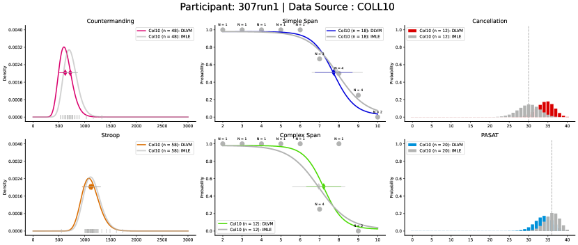
Figure 2: Median Fit of the trained DLVM model to the conventionally acquired COLL10 data (colored) compared with the IMLE fit to data (gray). The median fit was identified based on the log probability of the data given the predicted parameters by the DLVM model. Timing outputs in milliseconds (left column) were fit with log-normal distributions. Item response times are indicated by short vertical lines, means by diamonds and standard deviations by horizontal lines. Psychometric outputs (middle column) were fit by logistic sigmoids as a function of items to be remembered. Proportion correct for test times is indicated by circles, thresholds by diamonds and spreads by horizontal lines. Accurate completion of test items (right column) is fit by binomial distributions reflecting a hypothetical test containing 40 items. The proportion of test items successfully completed is indicated by vertical dashed lines.

In this section, we describe our results and demonstrate a DLVM model that successfully learned the correlations within the COLL10 data and performs well on unseen data. We compare our method against IMLE. Estimates generated by our method are labeled with DLVM whereas those generated by the traditional method are labeled with IMLE.

V-A Distribution fits for training Data

The trained DLVM model was able to capture the intra-participant and inter-participant correlations in the cognitive tests by projecting the observation (feature-space) performance to unique positions in the 3-dimensional latent space.

Figure 2 shows the median in-sample fit of the trained model across six different tasks. The DLVM fits are similar to the IMLE fits in this case, indicating that the trained model has learned a reasonable latent variable representation of the corresponding feature space of task outputs. The binomial distributions reflecting accuracy (i.e., PASAT and Cancellation) appear to be the least well aligned in this example, as well as the overall dataset. This observation can be at least partly attributable to the nature of the binomial distribution, in which central dispersion values are directly related to the total number of data points. The resolution of distributions reflecting accuracy tasks is therefore fundamentally limited by the amount of data available to fit them. The ability of DLVM to fit distributions using outside knowledge could represent an attractive alternative to the standard approach of accruing enough single-task data sufficiently removed from floor and ceiling effects to yield an interpretable accuracy score.

V-B Distribution fits for testing data

Figure 3 shows modeled test outputs for the median out-of-sample fit for both TB-IMLE (gray) and ML-DLVM (colors). Because TB-IMLE by definition can only use the data visible on each plot axis to train a model, the models and data would be expected to visibly correspond. That generally appears to be the case here. ML-DLVM is free of this constraint, however, and can incorporate other information deemed informative. In this case, the extra information incorporated into the model is how people generally perform on tests of this sort, as well as this individual’s performance on all the other tests in the battery.

The noticeable discrepancies in this case are worthy of additional inspection. Countermanding shows a number of long response times around 2 seconds in the TB-IMLE run, leading to a bimodal distribution. The effect of these long times in widening the lognormal distribution and raising its mean can be observed. Because the conventional single-task frequentist modeling framework does not allow outside information to be incorporated into the model, to alter the representation should would require labeling some data as “outliers” and excluding them from further analysis. Alternatively, one could collect larger amounts of data to empirically overwhelm outliers with valid data. The former strategy has the potential to increase estimator bias, while the latter strategy has the potential to increase estimator variance. Both strategies may ultimately reduce overall estimator error if applied properly. One of the main advantages of DLVM, however, is its ability manage the bias/variance tradeoff empirically, by allowing all data across all sessions and tasks to contribute to all distribution fits, as well as allowing an inductive bias via a Bayesian prior belief.

In this example, the actively acquired Countermanding data exhibited no obvious outliers. This might have occurred by chance or from the smaller overall number of active samples for this task or from the task-switching nature of DALE. In any case, the means of the two Countermanding distributions are concordant. A greater disparity is apparent for the Stroop means, but both model Stroop distributions appear generally reflective of their underlying data. A similar observation can be made for the Span models.

Greater discrepencies are apparent for the binomial models of task accuracy, however, as was the case for the in-sample example. This behavior is noticeable across the dataset, and could result from a multitude of factors. As noted above, tasks whose primary output is accuracy may be less well suited to DLVMs generally. Further research may be able to discern the relative utility of different tasks for constructing the latent variable models

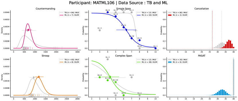
Figure 3: Distributions fitting test battery outputs for conventional test battery data (TB-IMLE, gray) and for machine learning test battery data (ML-DLVM, colors) for a median-fit participant (ID: MATML106). The median is based on the root-mean-square error (RMSE) between the IMLE and DLVM parameters. Plotting conventions as in Figure 2.

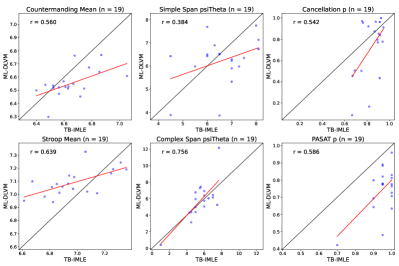
Figure 4: Similarity of primary test outputs (i.e., means and thresholds) between the conventional test battery + independent maximum likelihood estimation (TB-IMLE) and machine learning battery + distributional latent variable modeling (ML-DLVM). Timing task mean responses (left column) are in units of log milliseconds, psychometric task thresholds (center column) are in units of items recalled, and accuracy tasks (right column) are in units of probability correct. Numerical values are correlation coefficients.

V-C Similarity between TB-IMLE and ML-DLVM

The correspondence between the two testing procedures is quantified in Figure 4. As judged by the indicated correlation coefficients, correspondence is better for some tests than others. The Simple Span threshold exhibited the lowest correspondence with a correlation coefficient of $0.384$, for example, while the Complex Span threshold exhibited the highest correlation coefficient of $0.756$. Given that these two tasks are quite similar, the disparities in correlations across tasks do not seem to be attributable solely to task differences.

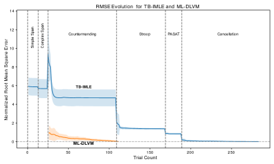
Figure 5: Comparison of average convergence rates toward final estimates for the conventional test battery + independent maximum likelihood estimation (TB-IMLE, blue) versus the machine learning battery with distributional latent variable modeling (ML-DLVM, orange). Values for the latter are only shown following primer sequence completion. Root-mean-square error values compared to final estimates were computed as proportion of the total range of each test output and summed. Lines are means across the cohort of 19 individuals while shaded areas represent ±1 standard deviation.

V-D Efficiency

The efficiency of DLVM compared to the conventional test battery can be seen in Figure 5. Substantial redundancy exists for the conventional test battery, with many tests proceeding long after the central tendency of the underlying distribution has been determined reasonably well. Note that DLVM is quantified only after it has completed its 26-sample primer sequence. The effect of this primer sequence appears to be able to place the latent variable position very close to its final position with 26 fixed test items. The modeling framework provides this efficiency boost, having learned from previous data how best to interpret a relatively small amount of incremental data from a new individual. Active learning provides the second boost, systematically probing the latent variable space for better representations by determining the best task item to deliver next.

V-E Test-retest reliability

Correspondence between repeats of the machine learning test battery within the same individual on different days for a different cohort of young adults is shown in Figure 6. Test-retest reliability overall is high, indicating both robustness of the underlying executive function construct over time as well as consistency of estimation. This outcome is particularly encouraging regarding this modeling approach given that the set of task items each day could be completely different. Further, DLVM is not specifically designed for test-retest reliability, only uncertainty minimization, making this result even more encouraging.

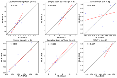
Figure 6: Similarity of primary test outputs between repeats of ML-DLVM on different days (A versus B). Plotting conventions as in Figure 4

Tasks with accuracy outputs (i.e., Cancellation and PASAT) give the poorest reliability. It is possible that these tasks are not particularly helpful at reducing uncertainty in other test results, either because they are inherently unreliable or poorly correlated with the other results or possibly both. One of the ancillary benefits of these machine learning methods is the ability to quantify the overall utility of very different testing procedures for their informativeness in representing cognitive performance. Further application of these methods may be able to identify absolute utility for different task categories in order to yield more informative test battery composition.

VI DISCUSSION AND FUTURE WORK

DLVM models evaluated using DALE achieve our goal of accommodating individual variation in cognitive test performance with accurate individualized cognitive models by leveraging both intrasubject and intersubject correlations. The results indicate that we are able to provide item-level predictions for each task and individual with fewer task items than is customarily delivered today. Even when trained with only the 26 primer data points, ML-DLVM is considerably better trained than is TB-IMLE with many more data points, as illustrated by Figure 5.

While this modeling framework makes effective use of individual data, it is also scalable to take advantage of population data when available, including much larger populations than demonstrated in this paper. Collectively, these achievements advance our long-term goal of providing rapid, equitable cognitive assessments for young students in order to design optimal math lessons for them on any given day. The substantially reduced testing times means that testing for a few minutes at the beginning of class each day may be sufficient to obtain actionable inference for daily individualized lesson planning.

Challenges and further work remain. The most substantial uncertainty is the overall accuracy of ML-DLVM as implemented. Generally speaking, primary test outputs for ML-DLVM at $\sim$100 samples compared against TB-IMLE at $\sim$280 samples with correlation coefficients of around 0.5–0.6 for a young adult population. Whether this value is above a target quality threshold depends on the particular application. It is possible that lower reliability of TB-IMLE in this cohort reduces the correlation values. Nevertheless, DLVM provides more flexibility for designing cognitive test batteries.

For the first time, we have constructed item-level latent-variable predictive models of intra-individual performance, complete with associated uncertainties. We have intentionally focused on evaluating predictive validity using individual test battery outputs, but other options are more attractive in the long run. In particular, the nature of the learned latent variable space itself should be reflective of relevant cognitive constructs. Future work will explore these latent variable spaces directly. Finally, we aim to make our method general and apply it to many applications suitable for latent variable modeling of distributional data.

References

- [1] O. Wilhelm, A. H. Hildebrandt, and K. Oberauer, “What is working memory capacity, and how can we measure it?” Frontiers in psychology, vol. 4, p. 433, 2013.
- [2] F. Schmiedek, M. Lövdén, and U. Lindenberger, “A task is a task is a task: putting complex span, n-back, and other working memory indicators in psychometric context,” Frontiers in psychology, vol. 5, p. 1475, 2014.
- [3] S. Weintraub, L. Besser, H. H. Dodge, M. Teylan, S. Ferris, F. C. Goldstein, B. Giordani, J. Kramer, D. Loewenstein, D. Marson et al., “Version 3 of the alzheimer disease centers’ neuropsychological test battery in the uniform data set (uds),” Alzheimer disease and associated disorders, vol. 32, no. 1, p. 10, 2018.
- [4] K. Lee, E. L. Ng, and S. F. Ng, “The contributions of working memory and executive functioning to problem representation and solution generation in algebraic word problems.” Journal of Educational Psychology, vol. 101, no. 2, p. 373, 2009.
- [5] R. Bull, K. A. Espy, S. A. Wiebe, T. D. Sheffield, and J. M. Nelson, “Using confirmatory factor analysis to understand executive control in preschool children: Sources of variation in emergent mathematic achievement,” Developmental science, vol. 14, no. 4, pp. 679–692, 2011.
- [6] M. B. Jurado and M. Rosselli, “The elusive nature of executive functions: A review of our current understanding,” Neuropsychology review, vol. 17, no. 3, pp. 213–233, 2007.
- [7] N. Akshoomoff, E. Newman, W. K. Thompson, C. McCabe, C. S. Bloss, L. Chang, D. G. Amaral, B. Casey, T. M. Ernst, J. A. Frazier et al., “The nih toolbox cognition battery: results from a large normative developmental sample (ping).” Neuropsychology, vol. 28, no. 1, p. 1, 2014.
- [8] S. Weintraub, S. S. Dikmen, R. K. Heaton, D. S. Tulsky, P. D. Zelazo, P. J. Bauer, N. E. Carlozzi, J. Slotkin, D. Blitz, K. Wallner-Allen et al., “Cognition assessment using the nih toolbox,” Neurology, vol. 80, no. 11 Supplement 3, pp. S54–S64, 2013.
- [9] K. Chaloner and I. Verdinelli, “Bayesian experimental design: A review,” Statistical Science, pp. 273–304, 1995.
- [10] D. A. Cohn, Z. Ghahramani, and M. I. Jordan, “Active learning with statistical models,” Journal of artificial intelligence research, vol. 4, pp. 129–145, 1996.
- [11] J. R. Gardner, X. Song, K. Q. Weinberger, D. L. Barbour, and J. P. Cunningham, “Psychophysical detection testing with bayesian active learning.” in UAI, 2015, pp. 286–295.
- [12] D. J. Bartholomew, M. Knott, and I. Moustaki, Latent variable models and factor analysis: A unified approach. John Wiley & Sons, 2011, vol. 904.
- [13] J. Vandekerckhove, “A cognitive latent variable model for the simultaneous analysis of behavioral and personality data,” Journal of Mathematical Psychology, vol. 60, pp. 58–71, 2014.
- [14] A. R. Conway, N. Cowan, M. F. Bunting, D. J. Therriault, and S. R. Minkoff, “A latent variable analysis of working memory capacity, short-term memory capacity, processing speed, and general fluid intelligence,” Intelligence, vol. 30, no. 2, pp. 163–183, 2002.
- [15] C. C. Aggarwal et al., “Neural networks and deep learning,” Springer, vol. 10, no. 978, p. 3, 2018.
- [16] N. P. Friedman and A. Miyake, “Unity and diversity of executive functions: Individual differences as a window on cognitive structure,” Cortex, vol. 86, pp. 186–204, 2017.
- [17] D. P. Kingma, M. Welling et al., “An introduction to variational autoencoders,” Foundations and Trends® in Machine Learning, vol. 12, no. 4, pp. 307–392, 2019.
- [18] A. Pahor, R. E. Mester, A. A. Carrillo, E. Ghil, J. F. Reimer, S. M. Jaeggi, and A. R. Seitz, “Ucancellation: A new mobile measure of selective attention and concentration,” Behavior research methods, vol. 54, no. 5, pp. 2602–2617, 2022.
- [19] A. Pahor, A. R. Seitz, and S. M. Jaeggi, “Near transfer to an unrelated n-back task mediates the effect of n-back working memory training on matrix reasoning,” Nature Human Behaviour, vol. 6, no. 9, pp. 1243–1256, 2022.
- [20] M. Rojo, P. Maddula, D. Fu, M. Guo, E. Zheng, A. Grande, A. Pahor, S. Jaeggi, A. Seitz, I. Goffney, G. Ramani, J. R. Gardner, and D. L. Barbour, “Scalable Probabilistic Modeling of Working Memory Performance,” N ov 2023. [Online]. Available: https://osf.io/preprints/psyarxiv/nq6yg/
- [21] M. Rojo, Q. W. Wong, A. Pahor, A. Seitz, S. Jaeggi, G. Ramani, I. Goffney, J. R. Gardner, and D. L. Barbour, “Accelerating Executive Function Assessments With Group Sequential Designs,” Nov 2023. [Online]. Available: https://osf.io/preprints/psyarxiv/mbtgk/