Ultra-high frequency primordial gravitational waves beyond the kHz:
the case of cosmic strings

Abstract

We investigate gravitational-wave backgrounds (GWBs) of primordial origin that would manifest only at ultra-high frequencies, from kilohertz to 100 gigahertz, and leave no signal at either LIGO, Einstein Telescope, Cosmic Explorer, LISA, or pulsar-timing arrays. We focus on GWBs produced by cosmic strings and make predictions for the GW spectra scanning over high-energy scale (beyond $10^{10}$ GeV) particle physics parameters. Signals from local string networks can easily be as large as the Big Bang nucleosynthesis/cosmic microwave background bounds, with a characteristic strain as high as $10^{-26}$ in the 10 kHz band, offering prospects to probe grand unification physics in the $10^{14}-10^{17}$ GeV energy range. In comparison, GWB from axionic strings is suppressed (with maximal characteristic strain $\sim 10^{-31}$) due to the early matter era induced by the associated heavy axions. We estimate the needed reach of hypothetical futuristic GW detectors to probe such GW and, therefore, the corresponding high-energy physics processes. Beyond the information of the symmetry-breaking scale, the high-frequency spectrum encodes the microscopic structure of the strings through the position of the UV cutoffs associated with cusps and/or kinks, as well as potential information about friction forces on the string. The IR slope, on the other hand, reflects the physics responsible for the decay of the string network. We discuss possible strategies for reconstructing the scalar potential, particularly the scalar self-coupling, from the measurement of the UV cutoff of the GW spectrum.

 

1 Primordial GWB at ultra-high frequencies

The landscape of gravitational waves (GW) in the ultra-high frequency (UHF) regime, above the kHz, is beyond the sensitivities of the present terrestrial experiments, LIGO/Virgo/KAGRA LIGOScientific:2014qfs ; LIGOScientific:2019vic , and planned, Einstein Telescope (ET) Hild:2010id ; Punturo:2010zz and Cosmic Explorer (CE) LIGOScientific:2016wof . It is compelling because it is clean from the standard astrophysical GW signals, such as binaries of massive objects Rosado:2011kv ; Sesana:2016ljz ; Lamberts:2019nyk ; Robson:2018ifk ; KAGRA:2021kbb ; KAGRA:2021vkt ; Babak:2023lro and would, in principle, be the reserved domain of early-Universe signals, ranging from primordial inflation Grishchuk:1974ny ; Starobinsky:1979ty ; Rubakov:1982df ; Bartolo:2016ami , thermal plasma Ghiglieri:2015nfa ; Ghiglieri:2020mhm ; Ringwald:2020ist ; Ghiglieri:2022rfp , first-order phase transitions Caprini:2015zlo ; Caprini:2019egz ; Gouttenoire:2022gwi , topological defects Vilenkin:2000jqa ; Blanco-Pillado:2017oxo ; Auclair:2019wcv ; Gouttenoire:2019kij , primordial black-holes Anantua:2008am ; Dolgov:2011cq ; Dong:2015yjs ; Franciolini:2022htd and preheating Easther:2006gt ; Garcia-Bellido:2007nns ; Garcia-Bellido:2007fiu ; Dufaux:2007pt ; Figueroa:2022iho ; Barman:2023ymn ; see reviews Caprini:2018mtu ; Renzini:2022alw ; LISACosmologyWorkingGroup:2022jok ; Simakachorn:2022yjy . The recently launched “UHF-GW Initiative” reviewed the detector concepts that have been proposed to explore this almost uncharted territory in Ref. Aggarwal:2020olq .

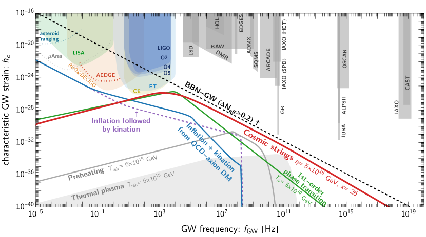
Figure 1: Benchmark GWBs of primordial origin with large amplitude above kHz frequencies, compared to sensitivities of existing and planned experiments below the kHz LISA:2017pwj ; LISACosmologyWorkingGroup:2022jok ; Yagi:2011wg ; AEDGE:2019nxb ; KAGRA:2013rdx ; LIGOScientific:2014qfs ; LIGOScientific:2019vic ; Hild:2010id ; Punturo:2010zz ; LIGOScientific:2016wof ; Blas:2021mqw ; Fedderke:2021kuy as well as experiments sensitive at frequencies above the kHz from Aggarwal:2020olq (in shaded gray). The green line is associated with a very strong first-order phase transition Caprini:2015zlo ($\beta/H=7$, $\alpha=10$) at a temperature $T\sim 10^{10}$ GeV (compatible with a Peccei-Quinn phase transition with axion decay constant $f_{a}\sim 10^{10}$ GeV for instance VonHarling:2019rgb ). Interestingly, the irreducible background from inflation with inflationary scale $E_{\rm inf}\simeq 10^{16}$ GeV can be amplified if inflation is followed by kination (purple line) Gouttenoire:2021jhk or if a kination era is induced much later by the rotating QCD axion DM field (blue line) Gouttenoire:2021wzu ; Gouttenoire:2021jhk ; Co:2021lkc . Local cosmic strings can generate a signal (in red) as large as the BBN bound (3), that also uniquely goes beyond $10^{9}$ Hz. The gray line shows the signal from preheating Figueroa:2022iho corresponding to an inflaton mass $M\simeq M_{\rm pl}$ with a coupling $g=10^{-3}$ to the thermal bath. Similar but suppressed GW spectra can come from the fragmentation of a scalar field, which is not the inflaton Kitajima:2018zco ; Chatrchyan:2020pzh ; Eroncel:2022vjg . The lower gray shaded region is the spectrum from the Standard thermal plasma Ghiglieri:2015nfa ; Ghiglieri:2020mhm ; Ringwald:2020ist , assuming a reheating temperature $T_{\rm reh}\simeq 6\times 10^{15}$ GeV.

The above primordial signals contribute to a stochastic gravitational-wave background (GWB) characterized by its frequency power spectrum, commonly expressed as the GW fraction of the total energy density of the Universe today $\Omega_{\rm GW}h^{2}$. It can be related to the characteristic strain $h_{c}$ of GW by Caprini:2018mtu

$$h_{c}\simeq 1.26\times 10^{-18}({\rm Hz}/f_{\rm GW})\sqrt{\Omega_{\rm GW}h^{2}}.$$ (1)

Its characteristic frequency is related to the moment when GW was emitted, and its amplitude is typically small ($\Omega_{\rm GW}h^{2}\lesssim\Omega_{r}h^{2}\simeq 4\cdot 10^{-5}$ Planck:2018vyg ).

The frequency range of cosmological GWB is linked to the size of the source, which is limited to the horizon size by causality. The frequency today of a GW produced with wavelength $\lambda_{\rm GW}\leq H^{-1}(T)$ when the Universe had temperature $T$ is

$$f_{\rm GW}\simeq 100~{}{\rm Hz}\left[\frac{H^{-1}(T)}{\lambda_{\rm GW}}\right]\left(\frac{T}{{10^{10}~{}\rm GeV}}\right),$$ (2)

where $H$ is the Hubble expansion rate assuming the standard $\Lambda$-cold-dark-matter (CDM) cosmology, and $f_{\rm GW}=\lambda_{\rm GW}[a(T)/a_{0}]$ with $a$ being the scale factor of cosmic expansion. For instance, the irreducible GWs produced during inflation that re-enter the horizon at temperature $T$ have $\lambda_{\rm GW}\sim H^{-1}$. On the other hand, GWs from first-order phase transitions have $\lambda_{\rm GW}$ that is roughly the bubbles’ size, typically of the order $\mathcal{O}(10^{-3}-10^{-1})H^{-1}$. GWs produced from the thermal plasma are produced maximally at $\lambda_{\rm GW}\sim T^{-1}$, such that the signal generated at any $T$ is peaked at $f_{\rm GW}\sim\mathcal{O}(10)$ GHz. Finally, for cosmic strings, $\lambda_{\rm GW}$ relates to the string-loop size which is fixed by the Hubble size; see Eq. (8) for the precise relation. Therefore, apart from the thermal plasma source, the highest GW frequencies are associated with the earliest moments in our history, and the maximum reheating temperature of the Universe $T_{\rm reh}\leq T_{\rm reh}^{\rm max}\simeq 6\times 10^{15}$ GeV Planck:2018jri bounds $f_{\rm GW}^{\rm max}\lesssim 10^{12}-10^{13}$ Hz for prime sources of cosmological GWBs.

As for the maximal amplitude of the GWB, there is a strong general constraint that applies at all frequencies. It comes from the maximally allowed amount of GW that can be present at the time of Big Bang nucleosynthesis (BBN) and in the cosmic microwave background (CMB) measurements Kawasaki:1999na ; Kawasaki:2000en ; Hannestad:2004px ; Planck:2018vyg . It can be written as the bound on the energy-density fraction in GW today $\Omega_{\rm GW}$ spanning over frequency $f_{\rm GW}$ as

$$\int_{f_{\rm GW}^{\rm min}}^{f_{\rm GW}^{\rm max}}\frac{df_{\rm GW}}{f_{\rm GW}}\,h^{2}\Omega_{\rm GW}(f_{\rm GW})\lesssim 5.6\times 10^{-6}\Delta N_{\rm eff},$$ (3)

where $h\simeq 0.68$ Planck:2018jri , the effective number $\Delta N_{\rm eff}\lesssim 0.2$ of relativistic particle species is bounded by BBN/CMB Mangano:2011ar ; Cyburt:2015mya ; Peimbert:2016bdg ; Planck:2018jri , and the $f_{\rm GW}^{\rm min}$ ($f_{\rm GW}^{\rm max}$) is the lower (upper) cutoff frequency of the GWB. This translates into $\Omega_{\rm GW}\lesssim 10^{-7}$ for short-lasting sources such as phase transitions, and to $\Omega_{\rm GW}\lesssim 10^{-8}$ for long-lasting sources such as cosmic strings; see Eq. (31). We compare in Fig. 1 different types of GW spectra inherited from the early universe, which would escape detection at present and future interferometers and would require UHF-GW experiments.

The interest in UHF-GW detection has blossomed lately, impulsed by the “UHF-GW Initiative” Aggarwal:2020olq , leading to new ideas for detection techniques, e.g., Ballantini:2005am ; Arvanitaki:2012cn ; Ejlli:2019bqj ; Aggarwal:2020umq ; LSD:2022mpz ; Berlin:2021txa ; Berlin:2022hfx ; Berlin:2023grv ; Goryachev:2021zzn ; Goryachev:2014yra ; Campbell:2023qbf ; Sorge:2023nax ; Tobar:2023ksi ; Carney:2023nzz ; Domcke:2022rgu ; Domcke:2023bat ; Bringmann:2023gba ; Vacalis:2023gdz ; Liu:2023mll ; Ito:2019wcb ; Ito:2020wxi ; Ito:2022rxn ; Ito:2023bnu . Still, this remains extremely challenging experimentally, and none of the proposals so far reach a sensitivity that enables them to go beyond the BBN bound (3). This paper aims to motivate further investigation and provide a concrete science case for UHF-GW detectors: the possibility to probe particle physics at energy scales many orders of magnitude beyond the reach of future particle colliders.

Cosmic strings Kibble:1976sj ; Kibble:1980mv ; Hindmarsh:1994re ; Vilenkin:2000jqa are among the most promising sources of GWBs; see Auclair:2019wcv ; Gouttenoire:2019kij for recent reviews. Not only do they arise in many well-motivated extensions of the Standard Model of particle physics, but they also scan almost the entire cosmological history. A string network evolves into the so-called scaling regime Kibble:1984hp ; Albrecht:1984xv ; Bennett:1987vf ; Bennett:1989ak ; Albrecht:1989mk ; Allen:1990tv ; Martins:2000cs ; Ringeval:2005kr ; Vanchurin:2005pa ; Martins:2005es ; Olum:2006ix ; Blanco-Pillado:2011egf ; Figueroa:2012kw ; Martins:2016ois where its energy density tracks the total energy density of the Universe, and continuously emits particles and string loops—where the latter subsequently decays into particles or radiates gravitationally Vachaspati:1984gt ; Vilenkin:1986ku ; Srednicki:1986xg ; Vilenkin:2000jqa ; Dabholkar:1989ju ; Vilenkin:1982ks .

With loops being produced throughout the cosmological history, the cosmic-string network is a long-lasting source of cosmological GWB, spanning an extremely broad frequency range. It carries information on the cosmic history prior to BBN, when the age of the Universe is less than $\sim$1 sec, and the energy scale is above $\sim$ MeV and far beyond. This GWB is potentially detectable at planned future GW experiments Janssen:2014dka ; EPTA:2015qep ; EPTA:2016ndq ; NANOGRAV:2018hou ; Weltman:2018zrl ; LISA:2017pwj ; LISACosmologyWorkingGroup:2022jok ; Yagi:2011wg ; LIGOScientific:2014qfs ; LIGOScientific:2019vic ; Hild:2010id ; Punturo:2010zz ; LIGOScientific:2016wof ; EPTA:2023hof ; EPTA:2023xxk ; NANOGrav:2023hvm ; Figueroa:2023zhu ; Ellis:2023oxs and its full spectrum could be reconstructed by space-based and ground-based GW observatories and their synergy Caprini:2019pxz ; Dimitriou:2023knw ; Alvey:2023npw . However, we will consider those GWB from cosmic strings that turn out to be unobservable at GW detectors below kHz frequencies due to their infrared (IR) cutoff. The current bound on the string tension $\mu$ [Eq. (4)] from pulsar timing arrays ($G\mu\lesssim 10^{-10}$ NANOGrav:2023hvm ; EPTA:2023xxk ; Figueroa:2023zhu ) and from LIGO/Virgo/KAGRA ($G\mu\lesssim 10^{-7}$ LIGOScientific:2021nrg ) are evaded in this case. The signals we will consider exceed the largest thermal-plasma GWB Ringwald:2020ist assuming the maximal reheating temperature $T_{\rm reh}^{\rm max}$.

We will discuss in turn local and global strings that result from the breaking of a local and global symmetry, respectively. The GWB from local cosmic strings can feature a low-frequency cutoff if the cosmic network decays—e.g., via monopole-antimonopole pair production Vilenkin:1982hm ; Copeland:1987ht ; Preskill:1992ck ; Vilenkin:2000jqa ; Monin:2008mp ; Leblond:2009fq —which could arise from multiple symmetry breakings in grand unified theories Lazarides:1981fv ; Kibble:1982ae ; Vilenkin:1982ks ; Vilenkin:1984ib . For global strings, which can be produced in postinflationary axion models, the metastability is automatically built-in and determined by the axion mass Vilenkin:1982ks ; Hiramatsu:2012gg . On the other hand, the high-frequency cutoffs depend on the symmetry-breaking scale when the network is formed, on the small-scale structures (kinks and cusps) of cosmic strings, and on the friction due to string interactions with the thermal plasma.

We briefly recap the cosmic-string GWB from a stable network in section 2 and the corresponding ultraviolet (UV) cutoffs in section 3. Then, section 4 focuses on the chopped GWB from local strings. Interestingly, we find a large GW signal in the UHF regime, which can be comparable to the BBN bound. In some cases, it exhibits a peak shape as opposed to the usual flat GWB from cosmic strings. Section 5 suggests ways to infer information about the underlying microscopic physics of cosmic strings from GW measurements at UHF-GW experiments. Section 6 discusses the case of global-string GWB from heavy axions. Considering the early temporary matter-domination (MD) era induced by decaying axions, we explain why detecting GWB from heavy-axion strings would be extremely challenging. We conclude in section 7. Appendices contain further details on (i) the peaked GWB spectrum in appendix A, (ii) the effect from the maximal mode of loop oscillation in appendix B, and (iii) the modified causality tail of axion-string GWB by the axion matter domination era in appendix C.

2 General properties of GWB from cosmic strings

We assume the existence of a complex scalar field $\Phi$, charged under a local or global $U(1)$-symmetry, with the potential $V(\Phi)=\lambda(|\Phi|^{2}-\eta^{2})^{2}/2$. The $U(1)$-symmetry is preserved at early times and gets spontaneously broken once the temperature drops below $T_{\rm form}\simeq\lambda^{1/2}\eta$ where $\eta$ is the vacuum expectation value of the field. This leads to the formation of the cosmic-string network with the string tension (i.e., energy per unit length) Vilenkin:2000jqa

$$\mu\simeq\eta^{2}\times\begin{cases}1~{}~{}&{\rm(local)},\\ \log(\lambda^{1/2}\eta/H)~{}~{}&{\rm(global)},\end{cases}$$ (4)

where $H$ is the Universe’s expansion rate. In this work, we remain agnostic on the string formation mechanism (either from thermal effects Kibble:1976sj ; Kibble:1980mv ; Hindmarsh:1994re ; Vilenkin:2000jqa or non-perturbative dynamics Kofman:1995fi ; Tkachev:1995md ; Kasuya:1997ha ; Kasuya:1998td ; Tkachev:1998dc ) and scan over the large range of string tension $\mu$. After the network formation, the string network keeps producing loops. It reaches the scaling regime where its energy density tracks the total energy density of the Universe, $\rho_{\rm net}(t)\simeq\mu/t^{2}\simeq G\mu\rho_{\rm tot}(t)$.

The produced loops decay into particles and GW. Local-string loops decay dominantly into GW while global-string loops decay dominantly into Goldstone radiation. The GWB in the high-frequency regime—corresponding to loop produced and emitting GW deep inside the radiation-dominated Universe—reads Gouttenoire:2019kij ; Gouttenoire:2021jhk

$$h^{2}\Omega_{\rm GW}\simeq\begin{cases}{\rm(local)}~{}1.5\cdot 10^{-10}\mathcal{G}[T(f_{\rm GW})]\\ ~{}~{}\times\left[\frac{G\mu}{10^{-11}}\right]^{\frac{1}{2}}\left[\frac{\alpha\times 50}{0.1\times\Gamma}\right]^{\frac{1}{2}},\\[5.0pt] {\rm(global)}~{}1.6\cdot 10^{-11}\left(\frac{\eta}{10^{15}\,\rm GeV}\right)^{4}\\ ~{}~{}\times\mathcal{G}[T(f_{\rm GW})]\left[\frac{\mathcal{D}(\eta,f_{\rm GW})}{94.9}\right]^{3}\left[\frac{C_{\rm eff}(f_{\rm GW})}{2.24}\right],\end{cases}$$ (5)

where $\alpha\sim\mathcal{O}(0.1)$ Blanco-Pillado:2013qja is the initial loop size as a fraction of Hubble horizon $H^{-1}$, $\Gamma\simeq 50$ Blanco-Pillado:2017oxo is the GW-emission efficiency, $\mathcal{G}(T)\equiv[g_{*}(T)/g_{*}(T_{0})][g_{*s}(T_{0})/g_{*s}(T)]^{4/3}$ with $g_{*}$ ($g_{*s}$) the relativistic degrees of freedom in energy (entropy) density and $T_{0}$ the photon temperature today. The parameter $C_{\rm eff}$ is the loop-production efficiency Gouttenoire:2019kij , and the log-correction is

$$\mathcal{D}(\eta,f_{\rm GW})=\log\left[5.7\cdot 10^{18}\left(\frac{\eta}{10^{15}\,\rm GeV}\right)\left(\frac{1\,\rm kHz}{f_{\rm GW}}\right)^{2}\right],$$ (6)

This work uses the exponent ‘3’ of the log-dependent term $\mathcal{D}$ (similar to Hindmarsh:2021vih ), although this is still under debate as the exponent ‘4’ is found in some simulation results Gorghetto:2018myk ; Gorghetto:2020qws ; Gorghetto:2021fsn . The final $\Omega_{\rm GW}$ in the latter case could be enhanced from our result due to the log factor by $\mathcal{O}(100)$. Note also that a potentially less efficient GW emission from a single loop was found in Baeza-Ballesteros:2023say , which suggests that $\Omega_{\rm GW}$ would be weaker by $\mathcal{O}(10^{4})$ compared to our result.

The GWB from local strings is $f_{\rm GW}$-independent, while the GWB from global-string GWB is log-suppressed at high frequencies. All GWB spectra in this work are calculated numerically by following Gouttenoire:2019kij where the number density of loops relies on the velocity-dependent one-scale (VOS) model Martins:1995tg ; Martins:1996jp ; Martins:2000cs ; Sousa:2013aaa ; Sousa:2014gka ; Correia:2019bdl . We show the GWB spectra from local strings in Fig. 2, where the IR and UV slopes are explained in the next sections. It is clear from this figure that large signals touching the BBN bound can arise, associated with $G\mu$ approaching $10^{-5}$ and thus a scale of $U(1)$ symmetry breaking close to $10^{16}$ GeV. We do not show the GWB spectra from global strings. As we shall see below, the metastability of heavy-axion strings comes with an early axion-matter-dominated era that dilutes and heavily suppresses the GWB.

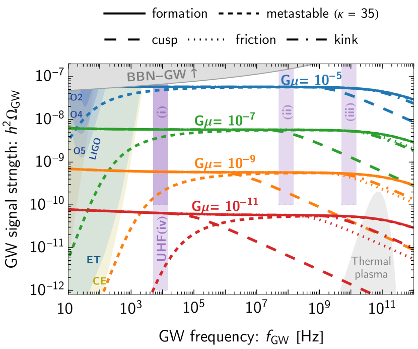
Figure 2: Local-string GWBs in the UHF range featuring different cutoffs. The solid lines show the stable-string GWB with the formation cutoff (10). The dashed, dotted, and dot-dashed lines correspond to the cutoffs from cusp (14), kink (15), and friction (19), respectively, assuming the stable-string network. The four rectangular purple regions denote hypothetical sensitivities of four fictional UHF-GW experiments; see Eq. (32). The “thermal plasma” gray region is the GWB predicted in Ghiglieri:2015nfa ; Ghiglieri:2020mhm ; Ringwald:2020ist , assuming the maximal reheating temperature $T_{\rm reh}^{\rm max}\simeq 6\times 10^{15}~{}{\rm GeV}$ Ghiglieri:2015nfa ; Ghiglieri:2020mhm ; Ringwald:2020ist , while the upper “bbn-gw” gray region is excluded by the BBN bound (3).

The broadband GWB spectrum is the result of the superposition of GW generated by many populations of loops produced at different temperatures. Each emits GW at frequency $f_{\rm GW}^{\rm emit}\simeq 2k/l$ Kibble:1982cb ; Hindmarsh:1994re where $k$ is the mode number of loop oscillation and the loop’s size is

$$l(t)=\alpha t_{i}-\Gamma G\mu(t-t_{i})$$ (7)

where $t_{i}$ is the time of loop formation. For the loop population created at temperature $T$, the GWB is sourced maximally at frequency today Gouttenoire:2019kij

$$f_{\rm GW}(T)\simeq\begin{cases}{\rm(local)}~{}2~{}{\rm kHz}\left[\frac{T}{10^{6}~{}\rm GeV}\right]\left[\frac{10^{-11}}{G\mu}\right]^{\frac{1}{2}}\left[\frac{g_{*}(T)}{g_{*}(T_{0})}\right]^{\frac{1}{4}},\\[5.0pt] {\rm(global)}~{}1.1~{}{\rm kHz}\left[\frac{T}{10^{8}~{}\rm GeV}\right]\left[\frac{g_{*}(T)}{106.75}\right]^{\frac{1}{4}}.\end{cases}$$ (8)

Note that the above frequency depends on $G\mu$ for local strings because the GW is sourced maximally around the time

$$\tilde{t}\simeq\alpha/(2\Gamma G\mu)t_{i}.$$ (9)

In contrast, global strings quickly emit GW after loop production $\tilde{t}\sim t_{i}$.

Eq. (8) indicates that the GW contribution at higher frequencies comes from smaller loops produced at higher energy where microscopic properties play a more prominent role. Ultimately, the GW emission, which relies on the collective motion of the smaller loops, is more suppressed Brandenberger:1986vj ; Blanco-Pillado:1998tyu . We now recap the different types of UV cutoffs in the next section; see also Auclair:2019jip for a review.

3 High-frequency cutoffs of cosmic-string GWB

A string-loop population contributes maximally to the GWB at the frequency in Eq. (8). It generates the UV tail with a slope of $\Omega_{\rm GW}\propto f_{\rm GW}^{-1}$ for a single proper loop-oscillation mode, both local and global strings; see Cui:2018rwi ; Gouttenoire:2019kij ; Simakachorn:2022yjy ; Ghoshal:2023sfa . Below the formation cutoff, the summation over large harmonics can be written as $\Omega_{\rm GW}^{\rm tot}=\sum_{k=1}^{k_{\rm max}}k^{-4/3}\Omega_{\rm GW}^{(1)}(f_{\rm GW}/k)$ where $\Omega_{\rm GW}^{(1)}$ is the first harmonic spectrum and $k_{\rm max}\to\infty$, the UV slope changes from $-1$ to $-1/3$ in the case of cusp loops Blasi:2020wpy ; Gouttenoire:2019kij . We show in appendix B and Fig. 12 that the precise calculation involving the $k$-dependent cutoff (due to the string’s width) leads to a slight modification in the slope above the UV cutoff and does not change the position of the cutoff (for $G\mu\lesssim 10^{-4}$). However, this is computationally expensive; therefore, in all figures, we apply that the spectra fall as $f_{\rm GW}^{-1/3}$ beyond the UV cutoffs, which we will now discuss.

3.1 Formation cut-off

The most conservative UV cutoff comes from the energy scale of the string-network formation. Using Eq. (8) with $T_{\rm form}\simeq\lambda^{1/2}$ $\eta\simeq\lambda^{1/2}$ $m_{\rm Pl}\sqrt{G\mu}$ where $m_{\rm Pl}=\sqrt{1/G}$ is the Planck mass, we obtain the formation cutoff for local strings,

$$\boxed{f_{\rm GW}^{\rm form}\simeq\begin{cases}{\rm\small(local)}~{}182~{}{\rm GHz}\,\sqrt{\lambda}\left[\frac{g_{*}(T_{\rm form})}{106.75}\right]^{\frac{1}{4}},\\[5.0pt] {\rm\small(global)}~{}11~{}{\rm GHz}\,\sqrt{\lambda}\left[\frac{\eta}{10^{15}~{}\rm GeV}\right]\left[\frac{g_{*}(T_{\rm form})}{106.75}\right]^{\frac{1}{4}}.\end{cases}}$$ (10)

Throughout this work, we set $\lambda=1$. For local strings, the formation cutoff does not depend on the string tension, as a higher GW frequency at production from an earlier network formation is compensated by the longer loop lifetime $\tilde{t}$. For global strings, the formation cutoff is proportional to the symmetry-breaking scale $\eta$, reflecting the fast decay of string loops.

3.2 Small-scale structures: kinks and cusps

The loops produced early are smaller and poorly approximated by the linelike description. Especially near small-scale structures such as cusps and kinks, they can dominantly decay via radiating non-perturbatively massive particles instead of emitting GW Brandenberger:1986vj ; Blanco-Pillado:1998tyu ; Olum:1998ag ; Matsunami:2019fss ; Blanco-Pillado:2023sap . Global string loops decay shortly after their formation such that a kink-collision or a cusp does not have time to develop. We therefore would not expect a cutoff on the global-string GWB spectrum from the cusp or kink, although this needs to be confirmed with numerical field-theory simulations. In this subsection, the formulae for cusp/kink cutoffs apply to local strings only.

The massive radiation is more efficient than the GW emission ($P_{\rm GW}=\Gamma G\mu$) when the loop length is smaller than $l_{m}=\beta_{m}{\mu^{-1/2}}/{\left(\Gamma G\mu\right)^{m}}$ where $m=1,~{}2$ for kink- and cusp-dominated loops, respectively Auclair:2019jip . The factor $\beta_{m}$ depends on the detailed small-scale structure of the string loop and typically grows with the number of kinks and cusps or the self-coupling $\lambda$. The overlapping cusp segment of length $\sqrt{wl}$ with the string width $w\simeq m_{\Phi}^{-1}\simeq(\lambda^{1/2}\eta)^{-1}$ annihilates into particles Brandenberger:1986vj ; Blanco-Pillado:1998tyu ; Olum:1998ag . The emission power per oscillation period $l/2$ is $P_{c}\sim N_{c}\mu\sqrt{wl}/l\simeq N_{c}\lambda^{-1/4}\mu^{3/4}/l^{1/2}$ with $N_{c}$ is the number of cusps which is typically two in each oscillation Blanco-Pillado:2015ana . The energy emission from kinks is $P_{k}\simeq N_{kk}\mu w/l\simeq N_{kk}\lambda^{-1/2}\mu^{1/2}/l$ with $N_{kk}$ is the number of kink-kink oscillation, which in some models can be as large as $N_{kk}\sim\mathcal{O}(10^{3}-10^{6})$ Ringeval:2017eww ; Binetruy:2010bq ; Binetruy:2010cc . Thus, we have

$$\beta_{c}\simeq N_{c}\lambda^{-1/4},~{}{\rm and}~{}\beta_{k}\simeq N_{kk}\lambda^{-1/2}.$$ (11)

The loops formed with a size $\alpha t_{i}$ smaller than $l_{m}$, or equivalently, formed above temperature

$$T_{\rm cusp} \simeq 0.59~{}{\rm PeV}\sqrt{\frac{1}{\beta_{c}}}\left(\frac{G\mu}{10^{-11}}\right)^{\frac{5}{4}}\left[\frac{106.75}{g_{*}(T)}\right]^{\frac{1}{4}},$$ (12)

$$T_{\rm kink} \simeq 26.2~{}{\rm EeV}\sqrt{\frac{1}{\beta_{k}}}\left(\frac{G\mu}{10^{-11}}\right)^{\frac{3}{4}}\left[\frac{106.75}{g_{*}(T)}\right]^{\frac{1}{4}}.$$ (13)

decay into massive particles with mass of order $\eta$ and should not contribute to the GWB Auclair:2019jip . We assume these subsequently decay into Standard Model particles and do not lead to additional constraints. Using Eq. (8) (where factor 2 is replaced by 45 not to include the later-time network evolution Gouttenoire:2019kij ), the GWB spectrum has the high-frequency cutoffs at Gouttenoire:2019kij

$$\boxed{f_{\rm GW}^{\rm cusp}\simeq 62.3~{}{\rm kHz}\sqrt{\frac{1}{\beta_{c}}}\left(\frac{G\mu}{10^{-11}}\right)^{3/4},}$$ (14)

$$\boxed{f_{\rm GW}^{\rm kink}\simeq 2.79~{}{\rm GHz}\sqrt{\frac{1}{\beta_{k}}}\left(\frac{G\mu}{10^{-11}}\right)^{1/4}.}$$ (15)

Using Eqs. (5), (14) and (15) and varying $G\mu$, the GW amplitude at the cutoffs are

$$h^{2}\Omega_{\rm GW}^{\rm kink} \simeq 7.35\times 10^{-12}~{}\beta_{k}\left(\frac{f_{\rm GW}^{\rm kink}}{1~{}{\rm GHz}}\right)^{2},$$ (16)

$$h^{2}\Omega_{\rm GW}^{\rm cusp} \simeq 3.69\times 10^{-10}~{}\beta_{c}^{\frac{1}{3}}\left(\frac{f_{\rm GW}^{\rm cusp}}{1~{}{\rm MHz}}\right)^{\frac{2}{3}}.$$ (17)

3.3 Thermal friction

Cosmic strings can experience a frictional force on top of the Hubble expansion if they interact with other particles of the thermal plasma. This friction affects the long-string evolution and also the oscillation of loops. The length scale for the efficient thermal friction is given by $l_{\rm fric}\sim\mu/(\sigma\rho_{\rm th})\equiv\mu/(\beta_{\rm fric}T^{3})$, where the scattering cross-section per unit length $\sigma\equiv\beta_{\rm fric}/T$ with $\beta_{\rm fric}$ depending on the nature of interactions Vilenkin:1991zk ; Vilenkin:2000jqa , and the energy density of thermal plasma $\rho_{\rm th}\sim T^{4}$. For example, the Aharonov-Bohm interaction induces friction with $\beta_{\rm fric}\sim 1$ Aharonov:1959fk ; Vilenkin:1991zk ; Vilenkin:2000jqa . Thermal friction is efficient at high $T$ until $2H\gtrsim l_{\rm fric}^{-1}$ when the temperature drops below

$$T_{\rm fric}\simeq 4.19~{}{\rm EeV}~{}\beta_{\rm fric}^{-1}\left(\frac{G\mu}{10^{-11}}\right)\left[\frac{g_{*}(T)}{106.75}\right]^{\frac{1}{2}}.$$ (18)

For local strings, this is associated with the frequency

$$\boxed{f_{\rm GW}^{\rm fric}\simeq 0.45~{}{\rm GHz}~{}\beta_{\rm fric}^{-1}\left(\frac{G\mu}{10^{-11}}\right)^{\frac{1}{2}}\left[\frac{g_{*}(T)}{106.75}\right]^{\frac{3}{4}},}$$ (19)

and the GW amplitude, when varying $G\mu$, follows

$$h^{2}\Omega_{\rm GW}^{\rm fric} \simeq 1.26\times 10^{-10}~{}\beta_{\rm fric}\left(\frac{f_{\rm GW}^{\rm fric}}{1~{}{\rm GHz}}\right).$$ (20)

The friction cutoff would carry information about the scalar field couplings to particles in the plasma. We will not discuss it for global strings since, as we will see, the UHF GWB from global axionic strings is not observable. In general, the GWB from cosmic strings is observable only at large string scales $\eta$ (corresponding to the axion decay constant $f_{a}$), which is severely constrained for the light axion Chang:2021afa ; Gorghetto:2021fsn ; Gorghetto:2023vqu ; Servant:2023mwt . For very heavy axions, we will show that a matter-domination era is induced, which suppresses the GWB further [see section 6].

UHF-GW experiments with sensitivity a few orders of magnitude below the BBN-GW bound would probe the nature of field theory at high energy scales. For example, as illustrated in Fig. 2, an experiment operating at $0.1$ GHz with $\Omega_{\rm sens}h^{2}\sim 10^{-8}$ [or characteristic strain $h_{c}\sim 10^{-30}$] would be able to probe the cusp cutoff of GWB from grand-unified-theory strings with $G\mu\sim[10^{-6},10^{-7}]$ or $\eta\sim[10^{15},10^{16}]$ GeV. Cosmic strings associated with such high values of $G\mu$ can be compatible with constraints from sub-kHz GW experiments if they are metastable Vilenkin:1982hm ; Preskill:1992ck ; Vilenkin:2000jqa ; Monin:2008mp ; Leblond:2009fq ; Dror:2019syi ; Buchmuller:2019gfy ; Buchmuller:2021mbb ; Buchmuller:2023aus . In the next section, we discuss metastable local strings, and in Section 6, we discuss metastable global strings.

Metastable local-string GWB

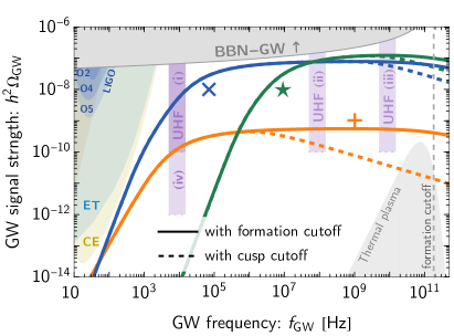
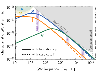
Figure 3: GWB spectra from metastable cosmic strings with the tension $G\mu$ and the metastability parameter $\kappa$ given by the three benchmark values in Fig. 5. The solid lines assume the GWB with formation cutoff indicated by the vertical dashed gray line, while the dashed lines assume the GWB with cusp cutoffs. The IR tails of the spectra exhibit the transition from $f_{\rm GW}^{2}$ to $f_{\rm GW}^{3}$ in the low-frequency direction; see Eq. (29). The top gray region denotes the BBN bound in Eq. (31). The bottom gray region is the thermal plasma GWB. The purple rectangles denote hypothetical GW experiments operating at the UHF range [defined by Eq. (32)], while other colored regions are the power-law integrated sensitivity curves of current and future GW observatories, taken from Gouttenoire:2019kij .

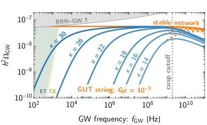
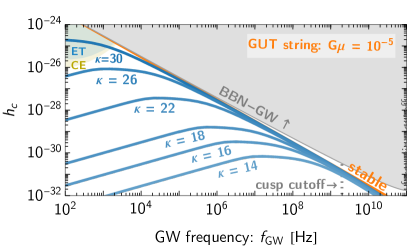
Figure 4: Local-string GWBs in blue with the metastability and cusp cutoffs, at fixed $G\mu=10^{-5}$, for different $\kappa$ where the dashed orange lines assume the cutoff from formation instead of the cusp. The spectrum exhibits a flat plateau shape when $f_{\rm GW}^{\rm meta}<f_{\rm GW}<f_{\rm GW}^{\rm cusp}$. For $f_{\rm GW}^{\rm meta}>f_{\rm GW}^{\rm cusp}$, the spectrum has a peak shape with the suppressed amplitude depending on the ratio $f_{\rm GW}^{\rm meta}/f_{\rm GW}^{\rm cusp}$ [see Eq. (33)].

4 Metastable local-string GWB: IR cutoff from monopoles

A theory leading to cosmic-string formation could be embedded in a theory with a symmetry group larger than $U(1)$ and which undergoes symmetry-breaking multiple times in the early Universe. We take the example of the local symmetry breaking pattern that gives rise to monopoles at high energy scale $m_{M}$ and cosmic strings at slightly smaller scale $\eta$ (see Buchmuller:2021mbb ; Buchmuller:2023aus for reviews on such theories and their GWB production). Note that the inflationary period between monopole and string formations is required to dilute the monopoles away.

4.1 Metastability cutoff

The metastability of the string network is induced by the nucleation of a monopole-antimonopole pair on strings via quantum tunneling with the rate per unit length $\Gamma_{d}=\frac{\mu}{2\pi}e^{-\pi\kappa}$ Leblond:2009fq with $\sqrt{\kappa}\equiv m_{M}/\eta$. This ratio is model-dependent; see for example Masoud:2021prr ; Buchmuller:2023aus . In this work, we treat $\kappa$ as a free parameter. The breakage of strings happens when $\Gamma_{d}\ell(t_{\rm brk})=H(t_{\rm brk})$. Using $\ell(t_{\rm brk})\simeq t_{\rm brk}$ and $H\sim 1/t$, we have

$$t_{\rm brk}\simeq\Gamma_{d}^{-\frac{1}{2}},$$ (21)

or equivalently, in the radiation era, for $H=T^{2}M_{\rm Pl}^{-1}\sqrt{\pi^{2}g_{*}/90}$,

$$T_{\rm brk}\simeq 1.74~{}{\rm TeV}\left[\frac{G\mu}{10^{-11}}\right]^{\frac{1}{4}}\left[\frac{106.75}{g_{*}(T)}\right]^{\frac{1}{4}}e^{-\frac{\pi}{4}(\kappa-36)},$$ (22)

Monopoles have two effects: (i) terminating loop production after $t_{\rm brk}$ and (ii) suppressing the number density of the existing loops. We will neglect the GWB from string segments, i.e., loops cut by monopoles, as it is subdominant to the GWB from loops Buchmuller:2021mbb . The modified number density of loops is Buchmuller:2021mbb ; Buchmuller:2023aus

$$n_{\rm loop}^{\rm brk}=n_{\rm loop}^{\rm stable}\Theta(t_{\rm brk}-t_{i})\mathcal{E}(l,t),$$ (23)

where $n_{\rm loop}^{\rm stable}$ is the loop number density of the stable network (obtained from the VOS model in this work), $t_{i}$ is the time of loop production, and the exponential suppression of the loop number density—as they break into monopoles over time—is Leblond:2009fq ; Buchmuller:2021mbb ; Buchmuller:2023aus

$$\mathcal{E}(l,t)=e^{-\Gamma_{d}\left[l(t)(t-t_{\rm brk})+\frac{1}{2}\Gamma G\mu\left(t-t_{\rm brk}\right)^{2}\right]}.$$ (24)

From this, one derives that the suppression of loop number density takes effect at the time

$$t_{\rm sup}\simeq\sqrt{2/(\Gamma_{d}\Gamma G\mu)}.$$ (25)

One might mistakenly associate the IR cutoff to the time $t_{\rm brk}$. In fact, the first population of loops that experiences number-density suppression and hence the suppressed GWB are loops contributing to GWB maximally at time $t_{\rm sup}$. These loops are produced at the time $t_{i}=2\Gamma G\mu t_{\rm sup}/\alpha$, using $\tilde{t}=t_{\rm sup}$ and Eq. (9). We arrive at the temperature,

$$T_{i,\rm sup}\simeq 4.9\times 10^{4}~{}{\rm GeV}\left[\frac{106.75}{g_{*}(T_{\rm sup})}\right]^{\frac{1}{4}}e^{-\frac{\pi}{4}(\kappa-36)},$$ (26)

Using Eq. (8) with $T_{i,\rm sup}$, the IR cutoff on the metastable-string GWB is at the frequency

$$\boxed{f_{\rm GW}^{\rm meta}\simeq 0.23~{}{\rm MHz}\left(\frac{10^{-11}}{G\mu}\right)^{\frac{1}{2}}e^{-\frac{\pi}{4}(\kappa-36)},}$$ (27)

where we multiply by the factor of $10^{3}$ to match the spectra obtained numerically. This accounts for non-linear $t$-dependence of $\mathcal{E}$ and the higher-mode summation such that the cutoff is defined where the amplitude drops by $\sim$50% from the stable-string prediction. For this reason, our Eq. (27) is different from Eq. (33) of Buchmuller:2021mbb by $\mathcal{O}(10^{2})$. The GWB spectrum changes from a flat shape for $f_{\rm GW}\gtrsim f_{\rm GW}^{\rm meta}$ to $\Omega_{\rm GW}\propto f_{\rm GW}^{2}$ for $f_{\rm GW}\lesssim f_{\rm GW}^{\rm meta}$ Buchmuller:2021mbb . When varying $G\mu$, the amplitude at the metastability cutoff follows

$$h^{2}\Omega_{\rm GW}^{\rm meta} \simeq 1.33\times 10^{-11}\left(\frac{1~{}{\rm MHz}}{f_{\rm GW}^{\rm meta}}\right)e^{-\frac{\pi}{4}(\kappa-36)}.$$ (28)

At frequency lower than the IR cutoff $f_{\rm GW}^{\rm meta}$, there is another characteristic scale corresponding to the GWB contribution from the last loop population formed at $T_{\rm brk}$ in Eq. (22); this is at frequency

$$\boxed{f_{\rm GW}^{\rm brk}\simeq 25~{}{\rm mHz}\left(\frac{G\mu}{10^{-11}}\right)^{\frac{1}{4}}e^{-\frac{\pi}{4}(\kappa-36)},}$$ (29)

where we use Eqs.  (8) and (22) and multiply by a factor of 0.01 to account for the effect of loop evolution and the higher-mode summation, such that it fits well the numerical result. Below $f_{\rm GW}^{\rm brk}$, the GWB spectrum is not generated by loops and is dominated by the causality tail ($\Omega_{\rm GW}\propto f_{\rm GW}^{3}$). Overall, the spectral shape of GWB from metastable local strings follows the asymptotic behavior

$$\Omega_{\rm GW}(f_{\rm GW})\propto\begin{cases}f_{\rm GW}^{3}~{}&{\rm for}~{}f_{\rm GW}\ll f_{\rm GW}^{\rm brk},\\ f_{\rm GW}^{2}~{}&{\rm for}~{}f_{\rm GW}^{\rm brk}\ll f_{\rm GW}\ll f_{\rm GW}^{\rm meta},\\ {\rm 1}~{}&{\rm for}~{}f_{\rm GW}^{\rm meta}\ll f_{\rm GW}\ll f_{\rm GW}^{\rm UV},\\ f_{\rm GW}^{-1/3}~{}&{\rm for}~{}f_{\rm GW}^{\rm UV}\ll f_{\rm GW}.\end{cases}$$ (30)

4.2 Large GWB in the UHF regime

Three benchmark GWB spectra of metastable strings are shown in Fig. 3, in units of the energy-density fraction $\Omega_{\rm GW}h^{2}$ as well as of the characteristic strain of GW $h_{c}$. We can see that the IR tails of these spectra follow the scaling $f_{\rm GW}^{2}$ and $f_{\rm GW}^{3}$, with the turning-point (29), as discussed above. These benchmark cases evade the current operating or planned GW experiments, as shown in Fig. 5. However, the entire parameter space above the kilohertz can be populated by the GWB from metastable strings.

The only upper bound on the GW amplitude comes from the BBN bound in Eq. (3). Using that the GWB shape is a flat plateau with the UV formation cutoff $f_{\rm GW}^{\rm form}$ and the IR metastability cutoff $f_{\rm GW}^{\rm meta}$, the “bbn-gw” becomes

$$h^{2}\Omega_{\rm GW}<\frac{5.6\times 10^{-6}\Delta N_{\rm eff}}{\log\left[\frac{f_{\rm GW}^{\rm form}}{\max\left(f_{\rm GW}^{\rm BBN},f_{\rm GW}^{\rm meta}\right)}\right]},$$ (31)

where $f_{\rm GW}^{\rm BBN}$ is the GW frequency at BBN scale [using $T_{\rm BBN}\simeq{\rm MeV}$ in Eq. (8)]. For illustrative purposes, we show the BBN bound of $h^{2}\Omega_{\rm GW}(f_{\rm GW}^{\rm meta})$ in gray regions in our figures. A UHF GW experiment with sensitivity a few orders of magnitude below the BBN bound would yield information about cosmic strings and monopoles in the early Universe.

To demonstrate the discovery potential of UHF-GW experiments, we assume some hypothetical experiments operating in the UHF regime with sensitivity and central frequency

$$\left\{\Omega_{\rm GW}^{\tt sens}h^{2},f_{\tt sens}\right\}~{}~{}{\rm within}~{}~{}\left[\frac{f_{\tt sens}}{2},\frac{3f_{\tt sens}}{2}\right],$$ (32)

which are shown as purple rectangles in the GWB spectra plots and purple lines in the parameter space plot of Fig. 5. We assume four benchmark sensitivities curves with $\left\{\Omega_{\rm GW}^{\tt sens}h^{2},f_{\tt sens}\right\}$ = (i) $\{10^{-10},10~{}{\rm kHz}\}$, (ii) $\{10^{-10},0.1~{}{\rm GHz}\}$, (iii) $\{10^{-10},10~{}{\rm GHz}\}$, and (iv) $\{10^{-12},10~{}{\rm kHz}\}$.

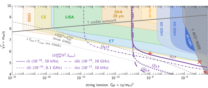
Figure 5: Future detectability regions of metastable local-string GWB by several experiments (only the gray region from the BBN bound and the dark blue from LIGO O2 are excluded). The criterion for detection and constraints is any part of the spectrum lying in the sensitivity and constrained regions. The purple solid, dashed, long-dashed, and dot-dashed lines illustrate the extended detectable region from hypothetical UHF experiments operating at different $\{\Omega_{\rm GW}^{\tt sens}h^{2},f_{\tt sens}\}$. The red symbols are associated with the benchmark GW spectra in Fig. 3. Assuming loops also produce particles through cusps, the dashed gray line marks the region where $f_{\rm GW}^{\rm brk}>f_{\rm GW}^{\rm cusp}$ and the GW is suppressed according to Eq. (33) [see also Fig. 4]. Below the gray dotted line ($T_{\rm brk}>T_{\rm cusp}$), all loops produced before the network decay release energy via particle production and thus do not generate GW signal. An earlier version of this plot appeared in Buchmuller:2019gfy ; we extended it by displaying the gained reach from UHF detectors.

4.3 Peak-shape GWB

The large GWB spectra allowed by metastability can exhibit an interesting “peak” shape when including the UV cutoffs of section 3. This happens if the IR cutoff from the metastability is lower than the UV cutoffs, i.e., $f_{\rm GW}^{\rm meta}\leq f_{\rm GW}^{\rm UV}$. This section focuses on the cusp cutoff (14), while this result can be easily extended to other UV cutoffs.

By imposing the cusp cutoff, the GWB from metastability gets suppressed into the $\Omega_{\rm GW}\propto f_{\rm GW}^{-1/3}$ scaling for $f_{\rm GW}>f_{\rm GW}^{\rm cusp}$. The GW spectrum peaks at the frequency $f_{\rm GW}^{\rm cusp}$ and has the approximated amplitude

$$\Omega_{\rm GW}^{\rm peak}\simeq\Omega_{\rm GW}^{\rm stable}\left({f_{\rm GW}^{\rm cusp}}/{f_{\rm GW}^{\rm meta}}\right)^{2},$$ (33)

assuming $f_{\rm GW}^{\rm cusp}>f_{\rm GW}^{\rm brk}$ [i.e., the IR tail retains the $\Omega_{\rm GW}\propto f_{\rm GW}^{2}$ scaling], otherwise one needs to account for the causality tail, discussed around Eq. (29). Using Eqs. (14) and (27), we have the suppression factor as $(f_{\rm GW}^{\rm cusp}/f_{\rm GW}^{\rm meta})^{2}\propto(G\mu)^{5/2}\exp(\pi\kappa/2)$. For a fixed $\kappa$, the peak-shape GWB is present for

$$\boxed{G\mu\lesssim 2.8\times 10^{-11}\,\beta_{c}^{2/5}e^{-\frac{\pi}{5}(\kappa-36)}~{}~{}{\rm(suppressed)}.}$$ (34)

Furthermore, all loops decay into particles rather than GW if $T_{\rm cusp}<T_{\rm brk}$, i.e.,

$$G\mu\lesssim 2.1\times 10^{-14}\,\sqrt{\beta_{c}}e^{-\frac{\pi}{4}(\kappa-36)}~{}~{}{\rm(no~{}GWB)},$$ (35)

where we use Eqs. (12) and (22). Fig. 4 shows examples of peak GWB spectra calculated numerically for a fixed $G\mu$, a similar plot with a fixed metastability parameter $\kappa$ is shown in Fig. 11 of appendix A. In Fig. 5, we indicate below the gray dashed line the region of parameter space where, due to the cusp cutoff, the GWB spectra are peak-shaped ($f_{\rm GW}^{\rm meta}>f_{\rm GW}^{\rm cusp}$), while below the dotted line, there is no GWB, corresponding to ($T_{\rm brk}>T_{\rm cusp}$).

As shown in Figs. 3 and 5, the GWB from metastable local strings can have a large amplitude in the UHF regime, saturating the BBN bound when the metastability parameter $\kappa$ is small enough. For example, the optimal benchmark point “$\times$” has $G\mu\simeq 10^{-5}$, corresponds to the GUT symmetry-breaking scale $\eta\sim 10^{16}~{}{\rm GeV}$, while the string formation scale is close to the monopole’s scale. Detecting any UV cutoff on the GWB spectrum will yield information about the nature of cosmic strings: the underlying field theory and its interactions. We will now investigate the possibility of reconstructing the scalar potential from the detectable UV cutoffs—using the UHF-GW experiments.

5 Reconstructing the scalar potential of cosmic strings

Given the discussion of the previous section, it is clear that the position of the UV cutoff depends on the parameters of the microscopic theory. Fig. 6 show the locations of the UV cutoffs when varying $G\mu$ from cusps, kinks, friction, and formation [Eqs. (10), (16), (17), and (20)] in the $\{f_{\rm GW},\Omega_{\rm GW}h^{2}\}$ plane. For each cutoff, we also show how the coefficients $\beta_{k}$, $\beta_{c}$, and $\beta_{\rm fric}$ change the positions of the cutoffs. The GWBs from stable strings are in yellow lines as references. For kink and cusp cutoffs, we vary $\beta_{c}$ and $\beta_{k}$ to values larger than 1 as they grow with a larger number of kinks and cusps and with smaller self-coupling $\lambda$, as shown in Eq. (11). We vary $\beta_{\rm fric}$, which is proportional to the interaction cross-section, from $10^{-3}$ to $10^{3}$.

By locating the cutoff, it is conceivable to infer from these measurements [using Eq. (11)], the values of parameters, such as the quartic coupling $\lambda$ of the scalar field as well as the vacuum expectation value $\eta$ which gives the scale of $U(1)$ symmetry breaking.

The possible strategy to pindown the cutoff’s position is to measure the GW spectrum at two different frequencies. If one detector can observe the flat part while the other observes the UV slope, we can deduce $G\mu$ (or $\eta$) and $\beta$ (once $G\mu$ is known), respectively. Fig. 7 shows the regions of the $\eta,\lambda,\beta_{\rm fric}$ parameter spaces that can be probed by the hypothetical UHF-GW experiments operating with $\Omega_{\rm GW}^{\tt sens}=10^{-10}$ and $f_{\rm GW}^{\tt sens}=$ (i) 10 kHz, (ii) 0.1 GHz, and (iii) 10 GHz. The gray dashed contours correspond to the characteristic strain $h_{c}^{\tt sens}$ of the detected signal. As an example, let us assume that the detector (i) sees a flat GWB with $h_{c}=10^{-26}$; that is $\eta\simeq 4\times 10^{15}$. Moreover, if the detector (iii) observes GWB with $h_{c}=10^{-32.5}$, we can infer that the cosmic strings have cuspy loops and the underlying scalar potential has $\eta=10^{15}$ GeV with $\lambda\simeq 10^{-8}$. From this particular observation, we would conclude the absence of a kink or a friction cutoff.

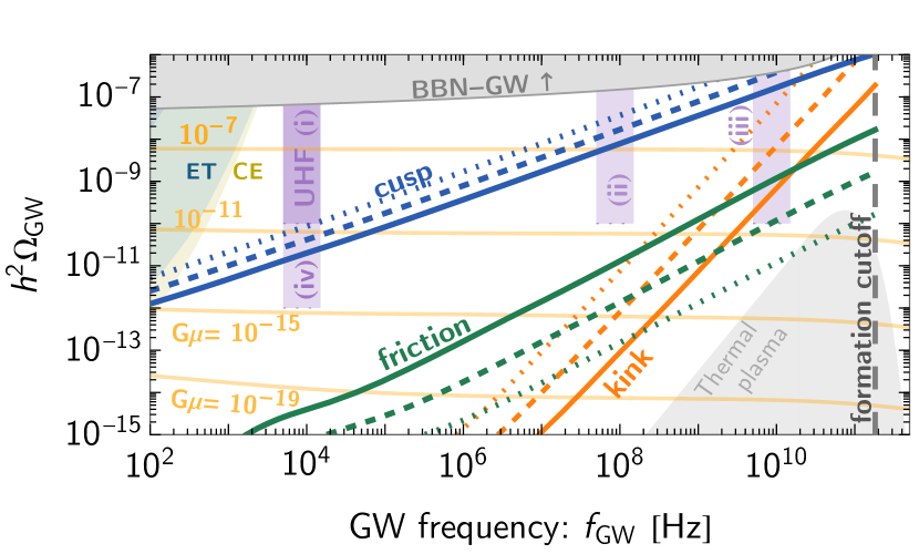
Figure 6: By varying the string tension $G\mu$, positions of the cutoffs—cusp, kink, and friction on the local-string GWB [see Eqs. (16), (17), and (20)]. For cusp and kink, the solid, dashed, and dotted lines correspond respectively to $\beta_{c},\beta_{k}$ = 1,10,100. The friction cutoff with $\beta_{\rm fric}=0.01,0.1,1$ is shown as solid, dashed, and dotted lines, respectively. The yellow spectra are those of the stable-string network with the formation cutoff.

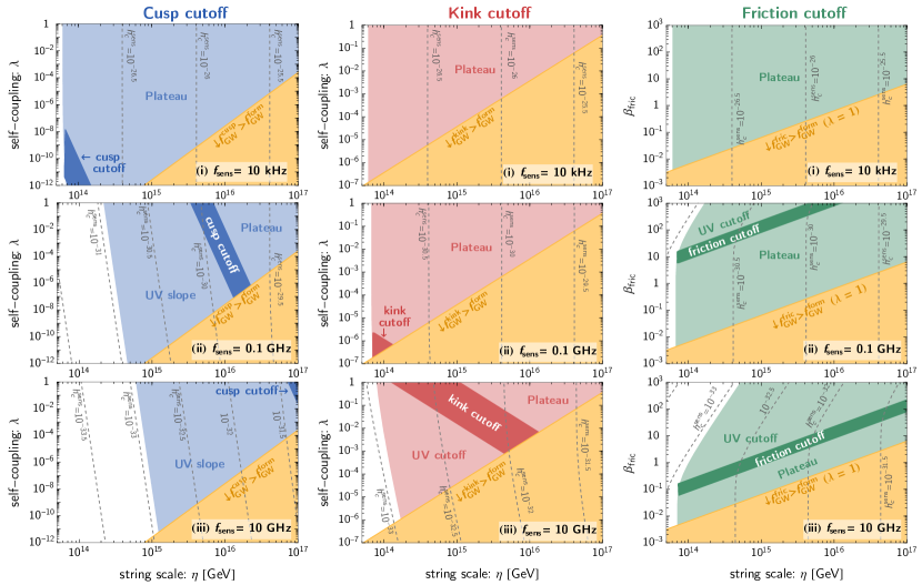
Figure 7: Colored region in each plot shows the detectable local-string GWB spectrum, including cusp (left-column), kink (middle-column), and friction (right-column) cutoffs. The detectable region splits into three parts depending on the feature of the GWB spectrum: the plateau (flat slope $\Omega_{\rm GW}\propto f_{\rm GW}^{0}$), the cutoff (where the slope changes), and the UV cutoff (slope $\Omega_{\rm GW}\propto f_{\rm GW}^{-1/3}$). We assume the hypothetical UHF experiments operating at $\Omega_{\rm GW}^{\tt sens}=10^{-10}$ with central frequencies: (i) 10 kHz, (ii) 0.1 GHz, and (iii) 10 GHz. The yellow region shows where these UV cutoffs are higher than the formation cutoff. The gray contours are the characteristic strain $h_{c}$ that would be detected in such experiments.

6 Metastable global-string GWB: heavy axions

Axion-string GWB

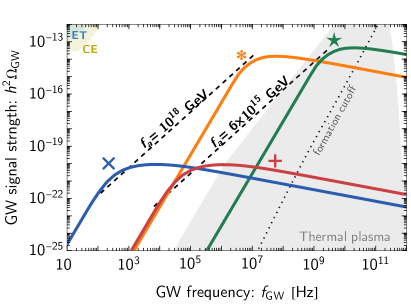
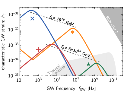
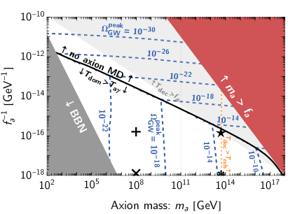
Figure 8: Top panel: GWB spectra in the energy-density fraction $\Omega_{\rm GW}h^{2}$ (left) and in the characteristic strain $h_{c}$ (right) corresponding to the benchmark $\{m_{a},f_{a}\}$ values in Fig. 8-bottom. The black dotted lines show the peak position of GWB spectrum for a constant $f_{a}$ while varying $m_{a}$ within the range where $m_{a}$ is allowed by $T_{a\gamma}$ above BBN and $T_{\rm dec}<T_{\rm reh}^{\rm max}$; see the bottom panel. The scaling of these lines follow $\Omega_{\rm GW}^{\rm peak}\propto(f_{\rm GW}^{\rm peak})^{8/5}$ and $h_{c}^{\rm peak}\propto(f_{\rm GW}^{\rm peak})^{-1/5}$ [see main text for derivation]. Bottom panel: Contours of the peak amplitude (left) and peak frequency (right) of the GW spectra, i.e., at $f_{\rm GW}(T_{\rm dec})$. We see that the GW from heavy-axion strings cannot generate an observable GW signal even for large $f_{a}$ due to the heavy dilution from the axion matter-dominated era. ($\star,*$ for $m_{a}=5\cdot 10^{13}$ GeV, $+,\times$ for $m_{a}=10^{8}$ GeV)

We now move to the case where the $U(1)$ symmetry is global; we can then identify the symmetry breaking scale $\eta$ to the axion decay constant $f_{a}$. When it breaks spontaneously after inflation at energy scale $f_{a}$ (so-called “post-inflationary” axion scenario), the network of global cosmic strings also forms loops and generates a GWB. The main difference with the local case is that the angular mode of the complex scalar field $\Phi$ associated with cosmic strings, the axion, is a Nambu-Golstone boson Peccei:1977hh ; Peccei:1977ur ; Weinberg:1977ma ; Wilczek:1977pj . It receives mass $m_{a}$ from axion shift-symmetry breaking dynamics and generates domain walls (DWs) Kibble:1976sj ; Kibble:1980mv ; Vilenkin:1982ks . After formation, DWs attach to cosmic strings and make them collapse entirely when $H\sim m_{a}$ Vilenkin:1982ks ; Hiramatsu:2012gg or equivalently at temperature

$$T_{\rm dec}\simeq 9\times 10^{8}~{}{\rm GeV}\left[\frac{106.75}{g_{*}(T_{\rm dec})}\right]^{\frac{1}{4}}\left(\frac{m_{a}}{\rm GeV}\right)^{\frac{1}{2}},$$ (36)

if the domain-wall number is unity.

The metastability of the cosmic-string network is therefore built-in automatically and can be included in the GWB calculation by introducing the cutoff in the loop number density after time $t_{\rm dec}\equiv t(T_{\rm dec})$

$$n_{\rm loop}^{\rm dec}=n_{\rm loop}^{\rm stable}\Theta(t_{\rm dec}-t_{i}),$$ (37)

where $t_{i}$ is the time when loops are produced, and $n_{\rm loop}^{\rm stable}$ is the loop number density of the stable network from the VOS model, calculated as in Gouttenoire:2019kij . Note that Eq. (37) is similar to the case of local strings in Eq. (23), except the factor $\mathcal{E}$ which suppresses loop density over time. The global-string loops decay quickly into GW and goldstone particles, such that the GW is determined by the number density of loops at the time of production $t_{i}$.

With no loop production below $T_{\rm dec}$, the GWB gets cut into the causality tail ($\Omega_{\rm GW}\propto f_{\rm GW}^{3}$) at frequency lower than

$$f_{\rm GW}^{\rm RD}(T_{\rm dec})\simeq 9.4~{}{\rm kHz}\left(\frac{\alpha}{0.1}\right)\left(\frac{m_{a}}{\rm GeV}\right)^{\frac{1}{2}},$$ (38)

using $T_{\rm dec}$ in Eq. (8) where the superscript “rd” reminds us that it assumes the radiation-dominated Universe at high energies as in the standard cosmological model. This is not always the case for the heavy axion, where the frequency can be further shifted by the axion matter-domination era; see below. The asymptotic behavior of the spectral shape is thus

$$\Omega_{\rm GW}(f_{\rm GW})\propto\begin{cases}f_{\rm GW}^{3}~{}&{\rm for}~{}f_{\rm GW}\ll f_{\rm GW}^{\rm dec},\\ \mathcal{D}^{3}~{}&{\rm for}~{}f_{\rm GW}\gg f_{\rm GW}^{\rm dec},\end{cases}$$ (39)

where $\mathcal{D}$ is the log-dependent factor defined in Eq. (6). That is, the GWB from metastable global strings exhibits a peak-shape spectrum, with peak frequency $f_{\rm GW}^{\rm RD}$ and peak amplitude $\Omega_{\rm GW}^{\rm RD,peak}$ estimated by Eq. (5). In this work, we determine the peak amplitude from the numerically generated GWB.

From Eq. (38), we find that the GWB from global axionic strings with axion mass $m_{a}\gtrsim 1~{}{\rm GeV}$ will not appear in GW experiments ($f_{\rm GW}\gtrsim 9~{}{\rm kHz}$) and could in principle be a well-motivated target for UHF-GW detectors. However, the decay of the string network produces heavy axions, which behave as non-relativistic matter and lead to an axion matter-domination (MD) era. We will discuss first the axion-MD era from the string-network decay and later the shifted and suppressed GWB.

6.1 Heavy axion matter-domination era

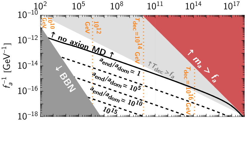
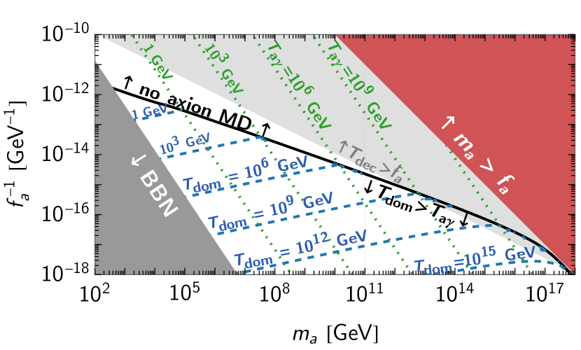
Figure 9: Parameter space of the heavy axion below the solid black line gives rise to the axion MD era with duration $a_{\rm end}/a_{\rm dom}$ [marked by the dashed black line], which decays before the BBN (otherwise, it is constrained as in the dark gray region.) The axions are produced from string-network decay as a subdominant energy density at $T_{\rm dec}$ (vertical dotted orange lines in the top panel). When they dominate the Universe, the axion MD era starts at $T_{\rm dom}$ (blue dashed lines) and later ends when they decay at $T_{a\gamma}$ (green dotted lines). The lighter gray region has the string network decaying before the string formation at temperature $f_{a}$. The perturbativity of the axion effective-field-theory description breaks down in the red region.

The string-wall network at $T_{\rm dec}$ having energy density $\rho_{\rm net}(T_{\rm dec})\simeq\mu(T_{\rm dec})/t_{\rm dec}^{2}\simeq G\mu(T_{\rm dec})\rho_{\rm tot}(T_{\rm dec})$ decays into non-relativistic axions (each of energy $\sim H\sim m_{a}$ Gelmini:2022nim ; Davis:1986xc ; Yamaguchi:1998gx ; Hiramatsu:2010yu ). Its energy density $\rho_{a}(T_{\rm dec})\simeq\rho_{\rm net}(T_{\rm dec})$ starts to redshift as $\rho_{a}\propto a^{-3}$ and dominates the thermal plasma energy density at temperature

$$T_{\rm dom}\simeq T_{\rm dec}G\mu(T_{\rm dec})\left[\frac{g_{*}(T_{\rm dec})g_{*s}(T_{\rm dom})}{g_{*}(T_{\rm dom})g_{*s}(T_{\rm dec})}\right],$$ (40)

leading to the axion MD era.

The axion MD era lasts until the axions decay, e.g., via $\mathcal{L}\supset-g\theta F\tilde{F}/4$ into SM photons which happens when the corresponding decay rate—$\Gamma_{a\gamma}=m_{a}^{3}g^{2}/(64\pi)$ Cadamuro:2011fd with $g_{a\gamma}={1.92\alpha_{\rm em}}/({2\pi f_{a}})$—is comparable to the Hubble rate. I.e., $\Gamma_{a\gamma}\simeq H_{\rm end}$ or equivalently at temperature

$$T_{a\gamma}\simeq 4.2~{}{\rm MeV}\left[\frac{106.75}{g_{*}(T_{a\gamma})}\right]^{\frac{1}{4}}\left(\frac{m_{a}}{\rm TeV}\right)^{\frac{3}{2}}\left[\frac{10^{12}~{}\rm GeV}{f_{a}}\right].$$ (41)

The axion MD exists if $T_{\rm dom}>T_{a\gamma}$ with the inverse duration, defined by

$$\boxed{\mathcal{B}\equiv\frac{a_{\rm dom}}{a_{\rm end}}=\left[\left(\frac{3\sqrt{10}}{64\pi^{2}}\right)\frac{m_{a}^{3}g_{a\gamma}^{2}M_{\rm Pl}}{g_{*}^{1/2}(T_{\rm dom})T_{\rm dom}^{2}}\right]^{\frac{2}{3}}\leq 1,}$$ (42)

which depends on the axion parameters as $\mathcal{B}\propto m_{a}^{4/3}f_{a}^{-4}$ [using Eqs. (36), (40)], up to the log-factor. Fig. 9 shows the heavy-axion parameter space $\{f_{a},m_{a}\}$, giving rise to the axion MD era that ends before BBN.

6.2 Strongly suppressed GW spectrum

The GWB from axion strings is produced until the string-network decay. The subsequent axion MD era dilutes both the amplitudes and frequencies of GWB because the Universe undergoes a longer expansion. To derive the modified GWB, let us consider the GW signals produced at temperature $T_{\rm emit}$ and frequency $f_{\rm GW}^{\rm emit}$. The frequency of the GW signal today is $f_{\rm GW}=f_{\rm GW}^{\rm emit}(a_{\rm emit}/a_{0})$; thus, we can relate the GW frequency in the presence of the axion MD to the one assuming the standard cosmological scenario $f_{\rm GW}^{\rm RD}$ in Eq. (38) as

$$\boxed{f_{\rm GW}=f_{\rm GW}^{\rm RD}\left[\frac{\mathcal{G}(T_{\rm end})}{\mathcal{G}(T_{\rm dom})}\right]^{\frac{1}{4}}\mathcal{B}^{\frac{1}{4}}.}$$ (43)

The energy density of GW signal redshifts as radiation $\Omega_{\rm GW}=({\rho_{\rm GW}^{\rm emit}}/{\rho_{\rm tot,0}})({a_{\rm emit}}/{a_{0}})^{4}$. So, the presence of the axion MD era dilutes the GW signal by

$$\boxed{\Omega_{\rm GW}(f_{\rm GW})=\Omega_{\rm GW}^{\rm RD}[f_{\rm GW}^{\rm RD}(f_{\rm GW})]\frac{\mathcal{G}(T_{\rm end})}{\mathcal{G}(T_{\rm dom})}\mathcal{B}.}$$ (44)

The GWB spectrum at frequencies higher than the IR cutoff gets diluted as a whole and retains its shape. However, below the cutoff, the causality tail of the GWB can also get modified at the frequencies corresponding to the horizon scale during the axion MD era, i.e., the scaling changes from $\Omega_{\rm GW}\propto f_{\rm GW}^{3}$ during radiation era to $\Omega_{\rm GW}\propto f_{\rm GW}$ during the matter era Hook:2020phx ; Racco:2022bwj . We find that the modified causality tail due to the axion MD era appears at extremely low amplitude, e.g., the change of slope at low $f_{\rm Gw}$ and small $h_{c}$ in the $*$ spectrum in Fig. 8-top-right. See more details about the modified causality tail in App. C and Fig. 13.

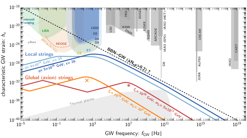
Figure 10: Maximal GWBs expected from cosmic strings (local in blue, global in red/orange) that can arise at ultra-high frequencies without leading to any observable signal in the frequency range of existing or planned interferometers. The spectra from global axionic strings can be large and detectable at lower frequencies for light axions Ramberg:2019dgi ; Chang:2019mza ; Gouttenoire:2019kij ; Gelmini:2021yzu ; Chang:2021afa ; Gorghetto:2021fsn ; Gelmini:2022nim ; Servant:2023mwt . However, when requiring a signal that arises only beyond the kHz, this fixes the axion mass to be above the GeV scale to avoid constraints from late decays after BBN. Such heavy axions induce an early temporary matter-domination era that suppresses the GWB.

Fig. 8-top shows the GWB spectra from the heavy-axion strings, corresponding to the benchmark points in Fig. 8-bottom and accounting already for the dilution from the axion-MD era. The gray dotted lines in Fig. 8-top estimate the peak position of GW spectrum of a constant $f_{a}$ [$\Omega_{\rm GW}^{\rm peak}\propto(f_{\rm GW}^{\rm peak})^{8/5}$ and $h_{c}^{\rm peak}\propto(f_{\rm GW}^{\rm peak})^{-1/5}$] deriving from Eq. (42) [$\mathcal{B}\propto m_{a}^{4/3}$], Eq. (38) [$f_{\rm GW}^{\rm RD}\propto m_{a}^{1/2}$], and Eq. (43). From Fig. 8-bottom, we see that the behavior of GW amplitude when there is no axion [i.e., $\Omega_{\rm GW}\propto f_{a}^{4}$ with a mild dependence on $m_{a}$ in Eq. (5)] changes to $f_{a}$-insensitive due to the axion MD era. Because the dilution factor $\mathcal{B}\propto f_{a}^{-4}$ ($T_{\rm dom}\propto\mu\propto f_{a}^{2}$) cancels the $f_{a}^{4}$-dependence of $\Omega_{\rm GW}^{\rm RD}$.

Limiting the string-decay temperature to the maximum reheating temperature (orange dotted line in Fig. 8-bottom), the benchmark ‘$\star$’ with $\{m_{a},f_{a}\}=\{5\cdot 10^{13}~{}{\rm GeV},4\cdot 10^{15}~{}{\rm GeV}\}$ gives the largest signal $\Omega_{\rm GW}h^{2}\simeq 10^{-14}$. Nonetheless, it is below the thermal plasma GWB (with $T_{\rm reh}^{\rm max}\simeq 6.6\times 10^{15}~{}{\rm GeV}$). On the other hand, the signal with maximum characteristic strain $h_{c}\simeq 10^{-31}$ is given by the axion mass of $m_{a}\simeq 10^{8}$ GeV and $f_{a}\simeq 10^{18}$ GeV. The associated benchmark spectrum is denoted ‘$\times$’ and has the peak frequency $\gtrsim$ kHz. In any case, the axion MD era suppresses the GWB from heavy-axion strings and renders its observability challenging.

7 Conclusion

The strongest current constraint on UHF GW comes from the $N_{\rm eff}$ bound (3). Future missions, such as CMB stage-4, will strengthen this bound. To get further insight on primordial GW would require experiments able to measure part of the spectral shape that encodes information on ultra high energy processes. We have shown that that there is a compelling science case for UHF-GW experiments operating with sensitivity slightly below the BBN bound. Grand Unification physics in the context of two-step symmetry-breaking events in the $10^{14}-10^{17}$ GeV energy range could lead to large signals close to the BBN bound. The maximal signals that can be expected from respectively local and global strings are plotted in the summary figure 10, which can be compared to Fig. 1 that displays other potential primordial sources of GWs at ultra high-frequencies. We have found that the GWB from global axionic strings is limited by the early matter era induced by heavy axions. Local cosmic strings on the other hand appear to be the most promising targets. From the GW amplitude, one can infer the scale of symmetry breaking, while the measurement of the UV cutoff of the GWB could provide microscopic information on the scalar field couplings.

Appendix A Peaked GWB

Complementary to Fig. 4 which shows the combined effects of the metastability and the cusp cutoffs for a given $G\mu$, Fig. 11 fixes the metastability parameter $\kappa$ and varies $G\mu$ instead. We see that the GWB spectra of $G\mu$ in Eq. (34)—corresponding to the GWB below where the two red lines cross—exhibit peak-shape feature.

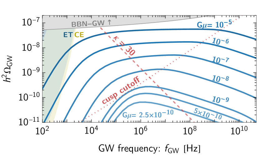
Figure 11: Local-string GWB spectra varying $G\mu$ in blue with the metastability ($\kappa=30$) and cusp cutoffs (in red). The spectrum exhibits a flat plateau shape when $f_{\rm GW}^{\rm meta}<f_{\rm GW}<f_{\rm GW}^{\rm cusp}$. For $f_{\rm GW}^{\rm meta}>f_{\rm GW}^{\rm cusp}$, the spectrum becomes a peak shape with the suppressed amplitude [see Eq. (33)].

Appendix B Effect of higher-mode summation

A string loop of length $l$ oscillates with frequency Vilenkin:2000jqa $\omega_{k}=4\pi k/l$ with a mode number $k$ and allows emission of energy $E_{k}=\omega_{k}$. The emission of energy from a loop should not change the string’s state by emitting energy larger than the mass of the scalar field, i.e., $E_{k}<\eta$ or $l>4\pi k/\eta$. That is, only a loop larger than $4\pi k/\eta$ supports the oscillation of mode $k$. Using that the loop length at formation is $l\simeq\alpha t$, we obtain that a mode $k$ oscillation is allowed on a loop below the temperature

$$T_{k}\simeq 8.3\times 10^{14}~{}{\rm GeV}\left(\frac{10^{-11}}{G\mu}\right)^{\frac{1}{4}}\left(\frac{1}{k}\right)^{\frac{1}{2}}.$$ (45)

Fig. 12-top shows the GWB spectrum from each mode $k$: $\Omega_{\rm GW}^{(k)}=k^{-4/3}\Omega_{\rm GW}^{\rm(1)}(f/k)$ where $\Omega_{\rm GW}^{\rm(1)}$ is the first-mode spectrum, and we consider only loops produced after $t_{i}>t(T_{k})$. For larger $k$, we see a more significant deviation between the spectra, including the effect of $T_{k}$ in Eq. (45), and those cut by the formation cutoff. In Fig. 12-bottom, we sum the spectra from $k=1$ up to $k=10^{3}$. The $T_{k}$ effect changes the UV slope of the spectrum at frequencies higher than the formation cutoff. It makes the slope of the UV tail steeper to the asymptotic slope of $\Omega_{\rm GW}\propto f_{\rm GW}^{-1}$. The reason is that, at higher frequencies, the contributions from large $k$-modes are more suppressed, and the first mode is responsible for the visible UV tail. As seen in Fig. 12-top, this effect is only relevant at frequencies above $10^{13}$ Hz and has no impact on observing the UV cutoffs, discussed in the main text. Although this effect might be relevant for the precise characterization of the signal’s far UV tail, the calculation is computationally expensive as one cannot use the rescaling technique: $\Omega_{\rm GW}^{\rm tot}=\sum_{k}k^{-4/3}\Omega_{\rm GW}^{(1)}(f/k)$. We will leave this aspect for future work.

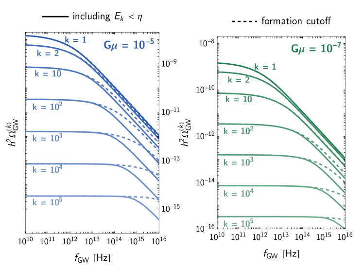
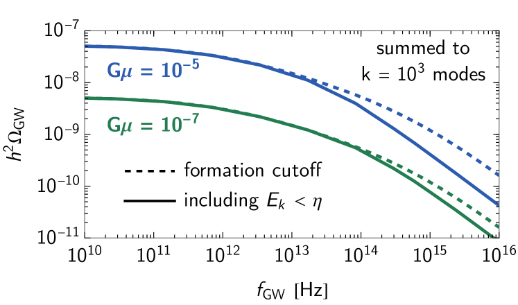
Figure 12: Top panel: The solid lines show GWB spectrum from each $k$-mode of loop oscillations, taking into account the limit on maximum emission energy; see Eq. (45). We compare this to the GWB spectra (dashed lines), assuming only the formation cutoff. Bottom panel: the total GW spectra, summing up to the first thousand modes.

Appendix C Modified causality tail of heavy-axion string GWB

Another effect of the axion MD era on the GWB from global strings is to modify the causality tail from the $\Omega_{\rm GW}\propto f_{\rm GW}^{3}$ scaling which assumes the radiation-domination era into the $\Omega_{\rm GW}\propto f_{\rm GW}$ during the matter era Hook:2020phx ; Racco:2022bwj ; Franciolini:2023wjm . The modification happens at the frequencies corresponding to the horizon scale during the axion MD era, i.e., $f_{\rm GW}^{H}=H[a(H)/a_{0}]$ with $H_{\rm dom}>H>H_{\rm end}$. We have

$$f_{\rm GW}^{H_{\rm end}}\simeq 18~{}{\rm nHz}\left[\frac{g_{*}(T_{\rm end})}{106.75}\right]^{\frac{1}{2}}\left[\frac{106.75}{g_{*s}(T_{\rm end})}\right]^{\frac{1}{3}}\left[\frac{T_{\rm end}}{1~{}{\rm GeV}}\right],$$ (46)

$${\rm and}~{}~{}~{}f_{\rm GW}^{H_{\rm dom}}\simeq f_{\rm GW}^{H_{\rm end}}\,\mathcal{B}^{-\frac{1}{2}}.$$ (47)

Fig. 13 shows the GW amplitudes of the modified causality tail at frequencies $f_{\rm GW}^{H_{\rm end}}$ and $f_{\rm GW}^{H_{\rm dom}}$. Although they fall in the sub-kHz range, the amplitude is too small to be detected by any current or future GW experiments.

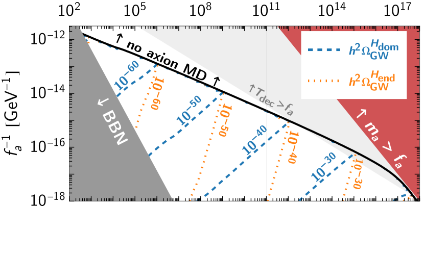
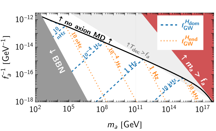
Figure 13: In the axion parameter space, the contour lines show amplitudes and frequencies of the modified causality tail of the axion-string GWB due to the axion MD era.

References

- (1) LIGO Scientific, VIRGO collaboration, Characterization of the LIGO detectors during their sixth science run, Class. Quant. Grav. 32 (2015) 115012 [1410.7764].
- (2) LIGO Scientific, Virgo collaboration, Search for the isotropic stochastic background using data from Advanced LIGO’s second observing run, Phys. Rev. D 100 (2019) 061101 [1903.02886].
- (3) S. Hild et al., Sensitivity Studies for Third-Generation Gravitational Wave Observatories, Class. Quant. Grav. 28 (2011) 094013 [1012.0908].
- (4) M. Punturo et al., The Einstein Telescope: A third-generation gravitational wave observatory, Class. Quant. Grav. 27 (2010) 194002.
- (5) LIGO Scientific collaboration, Exploring the Sensitivity of Next Generation Gravitational Wave Detectors, Class. Quant. Grav. 34 (2017) 044001 [1607.08697].
- (6) P. A. Rosado, Gravitational wave background from binary systems, Phys. Rev. D 84 (2011) 084004 [1106.5795].
- (7) A. Sesana, Prospects for Multiband Gravitational-Wave Astronomy after GW150914, Phys. Rev. Lett. 116 (2016) 231102 [1602.06951].
- (8) A. Lamberts, S. Blunt, T. B. Littenberg, S. Garrison-Kimmel, T. Kupfer and R. E. Sanderson, Predicting the LISA white dwarf binary population in the Milky Way with cosmological simulations, Mon. Not. Roy. Astron. Soc. 490 (2019) 5888 [1907.00014].
- (9) T. Robson, N. J. Cornish and C. Liu, The construction and use of LISA sensitivity curves, Class. Quant. Grav. 36 (2019) 105011 [1803.01944].
- (10) KAGRA, Virgo, LIGO Scientific collaboration, Upper limits on the isotropic gravitational-wave background from Advanced LIGO and Advanced Virgo’s third observing run, Phys. Rev. D 104 (2021) 022004 [2101.12130].
- (11) KAGRA, VIRGO, LIGO Scientific collaboration, GWTC-3: Compact Binary Coalescences Observed by LIGO and Virgo during the Second Part of the Third Observing Run, Phys. Rev. X 13 (2023) 041039 [2111.03606].
- (12) S. Babak, C. Caprini, D. G. Figueroa, N. Karnesis, P. Marcoccia, G. Nardini et al., Stochastic gravitational wave background from stellar origin binary black holes in LISA, JCAP 08 (2023) 034 [2304.06368].
- (13) L. P. Grishchuk, Amplification of gravitational waves in an istropic universe, Zh. Eksp. Teor. Fiz. 67 (1974) 825.
- (14) A. A. Starobinsky, Spectrum of relict gravitational radiation and the early state of the universe, JETP Lett. 30 (1979) 682.
- (15) V. A. Rubakov, M. V. Sazhin and A. V. Veryaskin, Graviton Creation in the Inflationary Universe and the Grand Unification Scale, Phys. Lett. B 115 (1982) 189.
- (16) N. Bartolo et al., Science with the space-based interferometer LISA. IV: Probing inflation with gravitational waves, JCAP 12 (2016) 026 [1610.06481].
- (17) J. Ghiglieri and M. Laine, Gravitational wave background from Standard Model physics: Qualitative features, JCAP 07 (2015) 022 [1504.02569].
- (18) J. Ghiglieri, G. Jackson, M. Laine and Y. Zhu, Gravitational wave background from Standard Model physics: Complete leading order, JHEP 07 (2020) 092 [2004.11392].
- (19) A. Ringwald, J. Schütte-Engel and C. Tamarit, Gravitational Waves as a Big Bang Thermometer, JCAP 03 (2021) 054 [2011.04731].
- (20) J. Ghiglieri, J. Schütte-Engel and E. Speranza, Freezing-In Gravitational Waves, 2211.16513.
- (21) C. Caprini et al., Science with the space-based interferometer eLISA. II: Gravitational waves from cosmological phase transitions, JCAP 04 (2016) 001 [1512.06239].
- (22) C. Caprini et al., Detecting gravitational waves from cosmological phase transitions with LISA: an update, JCAP 03 (2020) 024 [1910.13125].
- (23) Y. Gouttenoire, Beyond the Standard Model Cocktail, Springer Theses. Springer, Cham, 2022, 10.1007/978-3-031-11862-3, [2207.01633].
- (24) A. Vilenkin and E. P. S. Shellard, Cosmic Strings and Other Topological Defects. Cambridge University Press, 7, 2000.
- (25) J. J. Blanco-Pillado and K. D. Olum, Stochastic gravitational wave background from smoothed cosmic string loops, Phys. Rev. D 96 (2017) 104046 [1709.02693].
- (26) P. Auclair et al., Probing the gravitational wave background from cosmic strings with LISA, JCAP 04 (2020) 034 [1909.00819].
- (27) Y. Gouttenoire, G. Servant and P. Simakachorn, Beyond the Standard Models with Cosmic Strings, JCAP 07 (2020) 032 [1912.02569].
- (28) R. Anantua, R. Easther and J. T. Giblin, GUT-Scale Primordial Black Holes: Consequences and Constraints, Phys. Rev. Lett. 103 (2009) 111303 [0812.0825].
- (29) A. D. Dolgov and D. Ejlli, Relic gravitational waves from light primordial black holes, Phys. Rev. D 84 (2011) 024028 [1105.2303].
- (30) R. Dong, W. H. Kinney and D. Stojkovic, Gravitational wave production by Hawking radiation from rotating primordial black holes, JCAP 10 (2016) 034 [1511.05642].
- (31) G. Franciolini, A. Maharana and F. Muia, Hunt for light primordial black hole dark matter with ultrahigh-frequency gravitational waves, Phys. Rev. D 106 (2022) 103520 [2205.02153].
- (32) R. Easther and E. A. Lim, Stochastic gravitational wave production after inflation, JCAP 04 (2006) 010 [astro-ph/0601617].
- (33) J. Garcia-Bellido and D. G. Figueroa, A stochastic background of gravitational waves from hybrid preheating, Phys. Rev. Lett. 98 (2007) 061302 [astro-ph/0701014].
- (34) J. Garcia-Bellido, D. G. Figueroa and A. Sastre, A Gravitational Wave Background from Reheating after Hybrid Inflation, Phys. Rev. D 77 (2008) 043517 [0707.0839].
- (35) J. F. Dufaux, A. Bergman, G. N. Felder, L. Kofman and J.-P. Uzan, Theory and Numerics of Gravitational Waves from Preheating after Inflation, Phys. Rev. D 76 (2007) 123517 [0707.0875].
- (36) D. G. Figueroa, A. Florio, N. Loayza and M. Pieroni, Spectroscopy of particle couplings with gravitational waves, Phys. Rev. D 106 (2022) 063522 [2202.05805].
- (37) B. Barman, N. Bernal, Y. Xu and O. Zapata, Gravitational wave from graviton Bremsstrahlung during reheating, JCAP 05 (2023) 019 [2301.11345].
- (38) C. Caprini and D. G. Figueroa, Cosmological Backgrounds of Gravitational Waves, Class. Quant. Grav. 35 (2018) 163001 [1801.04268].
- (39) A. I. Renzini, B. Goncharov, A. C. Jenkins and P. M. Meyers, Stochastic Gravitational-Wave Backgrounds: Current Detection Efforts and Future Prospects, Galaxies 10 (2022) 34 [2202.00178].
- (40) LISA Cosmology Working Group collaboration, Cosmology with the Laser Interferometer Space Antenna, Living Rev. Rel. 26 (2023) 5 [2204.05434].
- (41) P. Simakachorn, Charting Cosmological History and New Particle Physics with Primordial Gravitational Waves, Ph.D. thesis, U. Hamburg (main), Hamburg U., 2022.
- (42) N. Aggarwal et al., Challenges and opportunities of gravitational-wave searches at MHz to GHz frequencies, Living Rev. Rel. 24 (2021) 4 [2011.12414].
- (43) LISA collaboration, Laser Interferometer Space Antenna, 1702.00786.
- (44) K. Yagi and N. Seto, Detector configuration of DECIGO/BBO and identification of cosmological neutron-star binaries, Phys. Rev. D 83 (2011) 044011 [1101.3940].
- (45) AEDGE collaboration, AEDGE: Atomic Experiment for Dark Matter and Gravity Exploration in Space, EPJ Quant. Technol. 7 (2020) 6 [1908.00802].
- (46) KAGRA, LIGO Scientific, Virgo, VIRGO collaboration, Prospects for observing and localizing gravitational-wave transients with Advanced LIGO, Advanced Virgo and KAGRA, Living Rev. Rel. 21 (2018) 3 [1304.0670].
- (47) D. Blas and A. C. Jenkins, Bridging the Hz Gap in the Gravitational-Wave Landscape with Binary Resonances, Phys. Rev. Lett. 128 (2022) 101103 [2107.04601].
- (48) M. A. Fedderke, P. W. Graham and S. Rajendran, Asteroids for Hz gravitational-wave detection, Phys. Rev. D 105 (2022) 103018 [2112.11431].
- (49) B. Von Harling, A. Pomarol, O. Pujolàs and F. Rompineve, Peccei-Quinn Phase Transition at LIGO, JHEP 04 (2020) 195 [1912.07587].
- (50) Y. Gouttenoire, G. Servant and P. Simakachorn, Kination cosmology from scalar fields and gravitational-wave signatures, 2111.01150.
- (51) Y. Gouttenoire, G. Servant and P. Simakachorn, Revealing the Primordial Irreducible Inflationary Gravitational-Wave Background with a Spinning Peccei-Quinn Axion, 2108.10328.
- (52) R. T. Co, D. Dunsky, N. Fernandez, A. Ghalsasi, L. J. Hall, K. Harigaya et al., Gravitational wave and CMB probes of axion kination, JHEP 09 (2022) 116 [2108.09299].
- (53) N. Kitajima, J. Soda and Y. Urakawa, Gravitational wave forest from string axiverse, JCAP 10 (2018) 008 [1807.07037].
- (54) A. Chatrchyan and J. Jaeckel, Gravitational waves from the fragmentation of axion-like particle dark matter, JCAP 02 (2021) 003 [2004.07844].
- (55) C. Eröncel, R. Sato, G. Servant and P. Sørensen, ALP dark matter from kinetic fragmentation: opening up the parameter window, JCAP 10 (2022) 053 [2206.14259].
- (56) Planck collaboration, Planck 2018 results. VI. Cosmological parameters, Astron. Astrophys. 641 (2020) A6 [1807.06209].
- (57) Planck collaboration, Planck 2018 results. X. Constraints on inflation, Astron. Astrophys. 641 (2020) A10 [1807.06211].
- (58) M. Kawasaki, K. Kohri and N. Sugiyama, Cosmological constraints on late time entropy production, Phys. Rev. Lett. 82 (1999) 4168 [astro-ph/9811437].
- (59) M. Kawasaki, K. Kohri and N. Sugiyama, MeV scale reheating temperature and thermalization of neutrino background, Phys. Rev. D 62 (2000) 023506 [astro-ph/0002127].
- (60) S. Hannestad, What is the lowest possible reheating temperature?, Phys. Rev. D 70 (2004) 043506 [astro-ph/0403291].
- (61) G. Mangano and P. D. Serpico, A robust upper limit on from BBN, circa 2011, Phys. Lett. B 701 (2011) 296 [1103.1261].
- (62) R. H. Cyburt, B. D. Fields, K. A. Olive and T.-H. Yeh, Big Bang Nucleosynthesis: 2015, Rev. Mod. Phys. 88 (2016) 015004 [1505.01076].
- (63) A. Peimbert, M. Peimbert and V. Luridiana, The primordial helium abundance and the number of neutrino families, Rev. Mex. Astron. Astrofis. 52 (2016) 419 [1608.02062].
- (64) R. Ballantini et al., Microwave apparatus for gravitational waves observation, gr-qc/0502054.
- (65) A. Arvanitaki and A. A. Geraci, Detecting high-frequency gravitational waves with optically-levitated sensors, Phys. Rev. Lett. 110 (2013) 071105 [1207.5320].
- (66) A. Ejlli, D. Ejlli, A. M. Cruise, G. Pisano and H. Grote, Upper limits on the amplitude of ultra-high-frequency gravitational waves from graviton to photon conversion, Eur. Phys. J. C 79 (2019) 1032 [1908.00232].
- (67) N. Aggarwal, G. P. Winstone, M. Teo, M. Baryakhtar, S. L. Larson, V. Kalogera et al., Searching for New Physics with a Levitated-Sensor-Based Gravitational-Wave Detector, Phys. Rev. Lett. 128 (2022) 111101 [2010.13157].
- (68) LSD collaboration, Optical Trapping of High-Aspect-Ratio NaYF Hexagonal Prisms for kHz-MHz Gravitational Wave Detectors, Phys. Rev. Lett. 129 (2022) 053604 [2204.10843].
- (69) A. Berlin, D. Blas, R. Tito D’Agnolo, S. A. R. Ellis, R. Harnik, Y. Kahn et al., Detecting high-frequency gravitational waves with microwave cavities, Phys. Rev. D 105 (2022) 116011 [2112.11465].
- (70) A. Berlin et al., Searches for New Particles, Dark Matter, and Gravitational Waves with SRF Cavities, 2203.12714.
- (71) A. Berlin, D. Blas, R. Tito D’Agnolo, S. A. R. Ellis, R. Harnik, Y. Kahn et al., Electromagnetic cavities as mechanical bars for gravitational waves, Phys. Rev. D 108 (2023) 084058 [2303.01518].
- (72) M. Goryachev, W. M. Campbell, I. S. Heng, S. Galliou, E. N. Ivanov and M. E. Tobar, Rare Events Detected with a Bulk Acoustic Wave High Frequency Gravitational Wave Antenna, Phys. Rev. Lett. 127 (2021) 071102 [2102.05859].
- (73) M. Goryachev and M. E. Tobar, Gravitational Wave Detection with High Frequency Phonon Trapping Acoustic Cavities, Phys. Rev. D 90 (2014) 102005 [1410.2334].
- (74) W. M. Campbell, M. Goryachev and M. E. Tobar, The multi-mode acoustic gravitational wave experiment: MAGE, Sci. Rep. 13 (2023) 10638 [2307.00715].
- (75) F. Sorge, High-Frequency Gravitational Waves in Electromagnetic Waveguides, Annalen Phys. 535 (2023) 2300228.
- (76) G. Tobar, S. K. Manikandan, T. Beitel and I. Pikovski, Detecting single gravitons with quantum sensing, 2308.15440.
- (77) D. Carney, V. Domcke and N. L. Rodd, Graviton detection and the quantization of gravity, 2308.12988.
- (78) V. Domcke, C. Garcia-Cely and N. L. Rodd, Novel Search for High-Frequency Gravitational Waves with Low-Mass Axion Haloscopes, Phys. Rev. Lett. 129 (2022) 041101 [2202.00695].
- (79) V. Domcke, C. Garcia-Cely, S. M. Lee and N. L. Rodd, Symmetries and Selection Rules: Optimising Axion Haloscopes for Gravitational Wave Searches, 2306.03125.
- (80) T. Bringmann, V. Domcke, E. Fuchs and J. Kopp, High-frequency gravitational wave detection via optical frequency modulation, Phys. Rev. D 108 (2023) L061303 [2304.10579].
- (81) G. Vacalis, G. Marocco, J. Bamber, R. Bingham and G. Gregori, Detection of high-frequency gravitational waves using high-energy pulsed lasers, Class. Quant. Grav. 40 (2023) 155006 [2301.08163].
- (82) T. Liu, J. Ren and C. Zhang, Detecting High-Frequency Gravitational Waves in Planetary Magnetosphere, 2305.01832.
- (83) A. Ito, T. Ikeda, K. Miuchi and J. Soda, Probing GHz gravitational waves with graviton–magnon resonance, Eur. Phys. J. C 80 (2020) 179 [1903.04843].
- (84) A. Ito and J. Soda, A formalism for magnon gravitational wave detectors, Eur. Phys. J. C 80 (2020) 545 [2004.04646].
- (85) A. Ito and J. Soda, Exploring high-frequency gravitational waves with magnons, Eur. Phys. J. C 83 (2023) 766 [2212.04094].
- (86) A. Ito and R. Kitano, Macroscopic Quantum Response to Gravitational Waves, 2309.02992.
- (87) T. W. B. Kibble, Topology of Cosmic Domains and Strings, J. Phys. A 9 (1976) 1387.
- (88) T. W. B. Kibble, Some Implications of a Cosmological Phase Transition, Phys. Rept. 67 (1980) 183.
- (89) M. B. Hindmarsh and T. W. B. Kibble, Cosmic strings, Rept. Prog. Phys. 58 (1995) 477 [hep-ph/9411342].
- (90) T. W. B. Kibble, Evolution of a system of cosmic strings, Nucl. Phys. B 252 (1985) 227.
- (91) A. Albrecht and N. Turok, Evolution of Cosmic Strings, Phys. Rev. Lett. 54 (1985) 1868.
- (92) D. P. Bennett and F. R. Bouchet, Evidence for a Scaling Solution in Cosmic String Evolution, Phys. Rev. Lett. 60 (1988) 257.
- (93) D. P. Bennett and F. R. Bouchet, Cosmic string evolution, Phys. Rev. Lett. 63 (1989) 2776.
- (94) A. Albrecht and N. Turok, Evolution of Cosmic String Networks, Phys. Rev. D 40 (1989) 973.
- (95) B. Allen and E. P. S. Shellard, Cosmic string evolution: a numerical simulation, Phys. Rev. Lett. 64 (1990) 119.
- (96) C. J. A. P. Martins and E. P. S. Shellard, Extending the velocity dependent one scale string evolution model, Phys. Rev. D 65 (2002) 043514 [hep-ph/0003298].
- (97) C. Ringeval, M. Sakellariadou and F. Bouchet, Cosmological evolution of cosmic string loops, JCAP 02 (2007) 023 [astro-ph/0511646].
- (98) V. Vanchurin, K. D. Olum and A. Vilenkin, Scaling of cosmic string loops, Phys. Rev. D 74 (2006) 063527 [gr-qc/0511159].
- (99) C. J. A. P. Martins and E. P. S. Shellard, Fractal properties and small-scale structure of cosmic string networks, Phys. Rev. D 73 (2006) 043515 [astro-ph/0511792].
- (100) K. D. Olum and V. Vanchurin, Cosmic string loops in the expanding Universe, Phys. Rev. D 75 (2007) 063521 [astro-ph/0610419].
- (101) J. J. Blanco-Pillado, K. D. Olum and B. Shlaer, Large parallel cosmic string simulations: New results on loop production, Phys. Rev. D 83 (2011) 083514 [1101.5173].
- (102) D. G. Figueroa, M. Hindmarsh and J. Urrestilla, Exact Scale-Invariant Background of Gravitational Waves from Cosmic Defects, Phys. Rev. Lett. 110 (2013) 101302 [1212.5458].
- (103) C. J. A. P. Martins, I. Y. Rybak, A. Avgoustidis and E. P. S. Shellard, Extending the velocity-dependent one-scale model for domain walls, Phys. Rev. D 93 (2016) 043534 [1602.01322].
- (104) T. Vachaspati and A. Vilenkin, Gravitational Radiation from Cosmic Strings, Phys. Rev. D 31 (1985) 3052.
- (105) A. Vilenkin and T. Vachaspati, Radiation of Goldstone Bosons From Cosmic Strings, Phys. Rev. D 35 (1987) 1138.
- (106) M. Srednicki and S. Theisen, Nongravitational Decay of Cosmic Strings, Phys. Lett. B 189 (1987) 397.
- (107) A. Dabholkar and J. M. Quashnock, Pinning Down the Axion, Nucl. Phys. B 333 (1990) 815.
- (108) A. Vilenkin and A. E. Everett, Cosmic Strings and Domain Walls in Models with Goldstone and PseudoGoldstone Bosons, Phys. Rev. Lett. 48 (1982) 1867.
- (109) G. Janssen et al., Gravitational wave astronomy with the SKA, PoS AASKA14 (2015) 037 [1501.00127].
- (110) EPTA collaboration, European Pulsar Timing Array Limits On An Isotropic Stochastic Gravitational-Wave Background, Mon. Not. Roy. Astron. Soc. 453 (2015) 2576 [1504.03692].
- (111) EPTA collaboration, High-precision timing of 42 millisecond pulsars with the European Pulsar Timing Array, Mon. Not. Roy. Astron. Soc. 458 (2016) 3341 [1602.08511].
- (112) NANOGRAV collaboration, The NANOGrav 11-year Data Set: Pulsar-timing Constraints On The Stochastic Gravitational-wave Background, Astrophys. J. 859 (2018) 47 [1801.02617].
- (113) A. Weltman et al., Fundamental physics with the Square Kilometre Array, Publ. Astron. Soc. Austral. 37 (2020) e002 [1810.02680].
- (114) EPTA collaboration, Practical approaches to analyzing PTA data: Cosmic strings with six pulsars, 2306.12234.
- (115) EPTA collaboration, The second data release from the European Pulsar Timing Array: V. Implications for massive black holes, dark matter and the early Universe, 2306.16227.
- (116) NANOGrav collaboration, The NANOGrav 15 yr Data Set: Search for Signals from New Physics, Astrophys. J. Lett. 951 (2023) L11 [2306.16219].
- (117) D. G. Figueroa, M. Pieroni, A. Ricciardone and P. Simakachorn, Cosmological Background Interpretation of Pulsar Timing Array Data, 2307.02399.
- (118) J. Ellis, M. Fairbairn, G. Franciolini, G. Hütsi, A. Iovino, M. Lewicki et al., What is the source of the PTA GW signal?, 2308.08546.
- (119) C. Caprini, D. G. Figueroa, R. Flauger, G. Nardini, M. Peloso, M. Pieroni et al., Reconstructing the spectral shape of a stochastic gravitational wave background with LISA, JCAP 11 (2019) 017 [1906.09244].
- (120) A. Dimitriou, D. G. Figueroa and B. Zaldivar, Fast Likelihood-free Reconstruction of Gravitational Wave Backgrounds, 2309.08430.
- (121) J. Alvey, U. Bhardwaj, V. Domcke, M. Pieroni and C. Weniger, Simulation-based inference for stochastic gravitational wave background data analysis, 2309.07954.
- (122) LIGO Scientific, Virgo, KAGRA collaboration, Constraints on Cosmic Strings Using Data from the Third Advanced LIGO–Virgo Observing Run, Phys. Rev. Lett. 126 (2021) 241102 [2101.12248].
- (123) A. Vilenkin, COSMOLOGICAL EVOLUTION OF MONOPOLES CONNECTED BY STRINGS, Nucl. Phys. B 196 (1982) 240.
- (124) E. J. Copeland, D. Haws, T. W. B. Kibble, D. Mitchell and N. Turok, Monopoles Connected by Strings and the Monopole Problem, Nucl. Phys. B 298 (1988) 445.
- (125) J. Preskill and A. Vilenkin, Decay of metastable topological defects, Phys. Rev. D 47 (1993) 2324 [hep-ph/9209210].
- (126) A. Monin and M. B. Voloshin, The Spontaneous breaking of a metastable string, Phys. Rev. D 78 (2008) 065048 [0808.1693].
- (127) L. Leblond, B. Shlaer and X. Siemens, Gravitational Waves from Broken Cosmic Strings: The Bursts and the Beads, Phys. Rev. D 79 (2009) 123519 [0903.4686].
- (128) G. Lazarides, Q. Shafi and T. F. Walsh, Cosmic Strings and Domains in Unified Theories, Nucl. Phys. B 195 (1982) 157.
- (129) T. W. B. Kibble, G. Lazarides and Q. Shafi, Strings in SO(10), Phys. Lett. B 113 (1982) 237.
- (130) A. Vilenkin, Cosmic Strings and Domain Walls, Phys. Rept. 121 (1985) 263.
- (131) T. Hiramatsu, M. Kawasaki, K. Saikawa and T. Sekiguchi, Production of dark matter axions from collapse of string-wall systems, Phys. Rev. D 85 (2012) 105020 [1202.5851].
- (132) L. Kofman, A. D. Linde and A. A. Starobinsky, Nonthermal phase transitions after inflation, Phys. Rev. Lett. 76 (1996) 1011 [hep-th/9510119].
- (133) I. I. Tkachev, Phase transitions at preheating, Phys. Lett. B 376 (1996) 35 [hep-th/9510146].
- (134) S. Kasuya and M. Kawasaki, Can topological defects be formed during preheating?, Phys. Rev. D 56 (1997) 7597 [hep-ph/9703354].
- (135) S. Kasuya and M. Kawasaki, Topological defects formation after inflation on lattice simulation, Phys. Rev. D 58 (1998) 083516 [hep-ph/9804429].
- (136) I. Tkachev, S. Khlebnikov, L. Kofman and A. D. Linde, Cosmic strings from preheating, Phys. Lett. B 440 (1998) 262 [hep-ph/9805209].
- (137) J. J. Blanco-Pillado, K. D. Olum and B. Shlaer, The number of cosmic string loops, Phys. Rev. D 89 (2014) 023512 [1309.6637].
- (138) M. Hindmarsh, J. Lizarraga, A. Lopez-Eiguren and J. Urrestilla, Approach to scaling in axion string networks, Phys. Rev. D 103 (2021) 103534 [2102.07723].
- (139) M. Gorghetto, E. Hardy and G. Villadoro, Axions from Strings: the Attractive Solution, JHEP 07 (2018) 151 [1806.04677].
- (140) M. Gorghetto, E. Hardy and G. Villadoro, More axions from strings, SciPost Phys. 10 (2021) 050 [2007.04990].
- (141) M. Gorghetto, E. Hardy and H. Nicolaescu, Observing invisible axions with gravitational waves, JCAP 06 (2021) 034 [2101.11007].
- (142) J. Baeza-Ballesteros, E. J. Copeland, D. G. Figueroa and J. Lizarraga, Gravitational Wave Emission from a Cosmic String Loop, I: Global Case, 2308.08456.
- (143) C. J. A. P. Martins and E. P. S. Shellard, String evolution with friction, Phys. Rev. D 53 (1996) 575 [hep-ph/9507335].
- (144) C. J. A. P. Martins and E. P. S. Shellard, Quantitative string evolution, Phys. Rev. D 54 (1996) 2535 [hep-ph/9602271].
- (145) L. Sousa and P. P. Avelino, Stochastic Gravitational Wave Background generated by Cosmic String Networks: Velocity-Dependent One-Scale model versus Scale-Invariant Evolution, Phys. Rev. D 88 (2013) 023516 [1304.2445].
- (146) L. Sousa and P. P. Avelino, Stochastic gravitational wave background generated by cosmic string networks: The small-loop regime, Phys. Rev. D 89 (2014) 083503 [1403.2621].
- (147) J. R. C. C. C. Correia and C. J. A. P. Martins, Extending and Calibrating the Velocity dependent One-Scale model for Cosmic Strings with One Thousand Field Theory Simulations, Phys. Rev. D 100 (2019) 103517 [1911.03163].
- (148) T. W. B. Kibble and N. Turok, Selfintersection of Cosmic Strings, Phys. Lett. B 116 (1982) 141.
- (149) R. H. Brandenberger, On the Decay of Cosmic String Loops, Nucl. Phys. B 293 (1987) 812.
- (150) J. J. Blanco-Pillado and K. D. Olum, Form of cosmic string cusps, Phys. Rev. D 59 (1999) 063508 [gr-qc/9810005].
- (151) P. Auclair, D. A. Steer and T. Vachaspati, Particle emission and gravitational radiation from cosmic strings: observational constraints, Phys. Rev. D 101 (2020) 083511 [1911.12066].
- (152) Y. Cui, M. Lewicki, D. E. Morrissey and J. D. Wells, Probing the pre-BBN universe with gravitational waves from cosmic strings, JHEP 01 (2019) 081 [1808.08968].
- (153) A. Ghoshal, Y. Gouttenoire, L. Heurtier and P. Simakachorn, Primordial black hole archaeology with gravitational waves from cosmic strings, JHEP 08 (2023) 196 [2304.04793].
- (154) S. Blasi, V. Brdar and K. Schmitz, Fingerprint of low-scale leptogenesis in the primordial gravitational-wave spectrum, Phys. Rev. Res. 2 (2020) 043321 [2004.02889].
- (155) K. D. Olum and J. J. Blanco-Pillado, Field theory simulation of Abelian Higgs cosmic string cusps, Phys. Rev. D 60 (1999) 023503 [gr-qc/9812040].
- (156) D. Matsunami, L. Pogosian, A. Saurabh and T. Vachaspati, Decay of Cosmic String Loops Due to Particle Radiation, Phys. Rev. Lett. 122 (2019) 201301 [1903.05102].
- (157) J. J. Blanco-Pillado, D. Jiménez-Aguilar, J. Lizarraga, A. Lopez-Eiguren, K. D. Olum, A. Urio et al., Nambu-Goto dynamics of field theory cosmic string loops, JCAP 05 (2023) 035 [2302.03717].
- (158) J. J. Blanco-Pillado, K. D. Olum and B. Shlaer, Cosmic string loop shapes, Phys. Rev. D 92 (2015) 063528 [1508.02693].
- (159) C. Ringeval and T. Suyama, Stochastic gravitational waves from cosmic string loops in scaling, JCAP 12 (2017) 027 [1709.03845].
- (160) P. Binetruy, A. Bohe, T. Hertog and D. A. Steer, Proliferation of sharp kinks on cosmic (super-)string loops with junctions, Phys. Rev. D 82 (2010) 083524 [1005.2426].
- (161) P. Binetruy, A. Bohe, T. Hertog and D. A. Steer, Gravitational wave signatures from kink proliferation on cosmic (super-) strings, Phys. Rev. D 82 (2010) 126007 [1009.2484].
- (162) A. Vilenkin, Cosmic string dynamics with friction, Phys. Rev. D 43 (1991) 1060.
- (163) Y. Aharonov and D. Bohm, Significance of electromagnetic potentials in the quantum theory, Phys. Rev. 115 (1959) 485.
- (164) C.-F. Chang and Y. Cui, Gravitational waves from global cosmic strings and cosmic archaeology, JHEP 03 (2022) 114 [2106.09746].
- (165) M. Gorghetto, E. Hardy, H. Nicolaescu, A. Notari and M. Redi, Early vs late string networks from a minimal QCD Axion, 2311.09315.
- (166) G. Servant and P. Simakachorn, Constraining postinflationary axions with pulsar timing arrays, Phys. Rev. D 108 (2023) 123516 [2307.03121].
- (167) J. A. Dror, T. Hiramatsu, K. Kohri, H. Murayama and G. White, Testing the Seesaw Mechanism and Leptogenesis with Gravitational Waves, Phys. Rev. Lett. 124 (2020) 041804 [1908.03227].
- (168) W. Buchmuller, V. Domcke, H. Murayama and K. Schmitz, Probing the scale of grand unification with gravitational waves, Phys. Lett. B 809 (2020) 135764 [1912.03695].
- (169) W. Buchmuller, V. Domcke and K. Schmitz, Stochastic gravitational-wave background from metastable cosmic strings, JCAP 12 (2021) 006 [2107.04578].
- (170) W. Buchmuller, V. Domcke and K. Schmitz, Metastable cosmic strings, JCAP 11 (2023) 020 [2307.04691].
- (171) M. A. Masoud, M. U. Rehman and Q. Shafi, Sneutrino tribrid inflation, metastable cosmic strings and gravitational waves, JCAP 11 (2021) 022 [2107.09689].
- (172) R. D. Peccei and H. R. Quinn, CP Conservation in the Presence of Instantons, Phys. Rev. Lett. 38 (1977) 1440.
- (173) R. D. Peccei and H. R. Quinn, Constraints Imposed by CP Conservation in the Presence of Instantons, Phys. Rev. D 16 (1977) 1791.
- (174) S. Weinberg, A New Light Boson?, Phys. Rev. Lett. 40 (1978) 223.
- (175) F. Wilczek, Problem of Strong and Invariance in the Presence of Instantons, Phys. Rev. Lett. 40 (1978) 279.
- (176) T. Hiramatsu, M. Kawasaki and K. Saikawa, Gravitational Waves from Collapsing Domain Walls, JCAP 05 (2010) 032 [1002.1555].
- (177) M. Kawasaki and K. Saikawa, Study of gravitational radiation from cosmic domain walls, JCAP 09 (2011) 008 [1102.5628].
- (178) T. Hiramatsu, M. Kawasaki, K. Saikawa and T. Sekiguchi, Axion cosmology with long-lived domain walls, JCAP 01 (2013) 001 [1207.3166].
- (179) T. Hiramatsu, M. Kawasaki and K. Saikawa, On the estimation of gravitational wave spectrum from cosmic domain walls, JCAP 02 (2014) 031 [1309.5001].
- (180) A. Hook, G. Marques-Tavares and D. Racco, Causal gravitational waves as a probe of free streaming particles and the expansion of the Universe, JHEP 02 (2021) 117 [2010.03568].
- (181) D. Racco and D. Poletti, Precision cosmology with primordial GW backgrounds in presence of astrophysical foregrounds, JCAP 04 (2023) 054 [2212.06602].
- (182) G. Franciolini, D. Racco and F. Rompineve, Footprints of the QCD Crossover on Cosmological Gravitational Waves at Pulsar Timing Arrays, 2306.17136.
- (183) G. B. Gelmini, A. Simpson and E. Vitagliano, Catastrogenesis: DM, GWs, and PBHs from ALP string-wall networks, JCAP 02 (2023) 031 [2207.07126].
- (184) R. L. Davis, Cosmic Axions from Cosmic Strings, Phys. Lett. B 180 (1986) 225.
- (185) M. Yamaguchi, M. Kawasaki and J. Yokoyama, Evolution of axionic strings and spectrum of axions radiated from them, Phys. Rev. Lett. 82 (1999) 4578 [hep-ph/9811311].
- (186) T. Hiramatsu, M. Kawasaki, T. Sekiguchi, M. Yamaguchi and J. Yokoyama, Improved estimation of radiated axions from cosmological axionic strings, Phys. Rev. D 83 (2011) 123531 [1012.5502].
- (187) D. Cadamuro and J. Redondo, Cosmological bounds on pseudo Nambu-Goldstone bosons, JCAP 02 (2012) 032 [1110.2895].
- (188) N. Ramberg and L. Visinelli, Probing the Early Universe with Axion Physics and Gravitational Waves, Phys. Rev. D 99 (2019) 123513 [1904.05707].
- (189) C.-F. Chang and Y. Cui, Stochastic Gravitational Wave Background from Global Cosmic Strings, Phys. Dark Univ. 29 (2020) 100604 [1910.04781].
- (190) G. B. Gelmini, A. Simpson and E. Vitagliano, Gravitational waves from axionlike particle cosmic string-wall networks, Phys. Rev. D 104 (2021) 061301 [2103.07625].