The Guided Moments formalism: a new efficient full-neutrino treatment for astrophysical simulations

Abstract

We present the new Guided Moments (GM) formalism for neutrino modeling in astrophysical scenarios like core-collapse supernovae and neutron star mergers. The truncated moments approximation (M1) and Monte-Carlo (MC) schemes have been proven to be robust and accurate in solving the Boltzmann’s equation for neutrino transport. However, it is well-known that each method exhibits specific strengths and weaknesses in various physical scenarios. The GM formalism effectively solves these problems, providing a comprehensive scheme capable of accurately capturing the optically thick limit through the exact M1 closure and the optically thin limit through a MC based approach. In addition, the GM method also approximates the neutrino distribution function with a reasonable computational cost, which is crucial for the correct estimation of the different neutrino-fluid interactions. Our work provides a comprehensive discussion of the formulation and application of the GM method, concluding with a thorough comparison across several test problems involving the three schemes (M1, MC, GM) under consideration.

I Introduction

The coalescence of neutron stars is an extraordinary phenomenon in high-energy astrophysics, occurring in extreme environments marked by strong self-gravity, high densities, and elevated temperatures. The simultaneous detection of gravitational waves (GWs) and electromagnetic (EM) signals from binary neutron stars (BNS), exemplified by the groundbreaking GW170817 event (Abbott et al. 2017a; Abbott et al. 2017b), shows the potential of multi-messenger astronomy. Numerous detections of GWs and EM signals from neutron star mergers are expected in the coming years (see, for instance, Colombo et al. 2022). The observation of such signals is predicted to have a profound impact on both astrophysics and fundamental physics. Nevertheless, the complexity of modeling all the involved physical interactions constrains our capacity to realistically simulate these binary mergers and compare them with present observations. Unraveling the physics embedded in these signals requires solving, at least approximately, the general relativistic radiation magneto-hydrodynamic equations: Einstein equations for depicting strong gravity, relativistic magnetohydrodynamics (MHD) to model magnetized fluids, and Boltzmann’s equation to describe the production and transport of neutrinos. Obtaining accurate solutions for these equations, in realistic general astrophysical settings like neutron star mergers, is an exceedingly challenging task which can solely be addressed through numerical simulations.

After the merger, a massive neutron star or a black hole, surrounded by a strongly magnetized hot and dense accretion torus is likely to be formed (see, for instance, Kiuchi et al. 2018; Foucart 2023). Throughout the coalescence, various regions may experience conditions ranging from the optically thin regime, characterized by freely streaming neutrinos, to the optically thick regime, where neutrinos are mostly trapped and propagate through diffusion. Due to their substantial energies and luminosities, neutrinos are expected to play a fundamental role in physical processes in the post-merger phase of a neutron star merger (for an extensive review, see Foucart 2023). In particular, neutrino interactions are expected to induce changes in matter composition, influencing the conditions relevant to the $r$-process nucleosynthesis (e.g., Lippuner and Roberts 2015; Just et al. 2015a; Thielemann et al. 2017; Perego et al. 2020). Neutrinos produced in hot and dense matter regions will diffuse and eventually decouple from the fluid at lower densities, being emitted from the system while carrying away energy. As neutrinos extract energy from the system, they could give rise to additional matter outflows, manifested as neutrino-driven winds (e.g., Dessart et al. 2008; Perego et al. 2014; Fujibayashi et al. 2017; Fujibayashi et al. 2020).

Accurately capturing all these phenomena in neutron star merger simulations require an accurate and realistic treatment of neutrino transport in numerical relativity (NR) codes (Foucart et al. 2022). This task involves the tremendous challenge of solving the 7-dimensional Boltzmann’s equation, which describes the evolution of a distribution function for each neutrino species. To address this complexity, several approaches, including direct and approximate methods have been explored. Presently, various methods directly attempt to solve the full Boltzmann’s equation in full GR, using Monte-Carlo (MC) based approaches (see, for example, Abdikamalov et al. 2012; Richers et al. 2015; Ryan et al. 2015; Foucart 2018; Foucart et al. 2018; Ryan and Dolence 2020; Foucart et al. 2021; Kawaguchi et al. 2023; Foucart et al. 2023), lattice-Boltzmann methods (Weih et al. 2020a), expansion of momentum-space distributions into spherical harmonics ($P_{n}$) methods (see, e.g., Pomraning 1973; McClarren and Hauck 2010; Radice et al. 2013a), discrete-ordinates ($S_{n}$) methods (see, e.g., Pomraning 1969; Mihalas and Weibel-Mihalas 1999; Chan and Müller 2020a) and a finite element approach in angle (Bhattacharyya and Radice 2023). Direct methods, although expected to converge to the true solution, often present challenges in their implementation and computational cost, making them in most of the cases impractical for providing a numerical solution with sufficient accuracy. A notable example is the handling of the optically thick regime in the Monte-Carlo based methods, where resolving the small neutrino mean-free path becomes challenging, often requiring further simplifications (see, for instance, Fleck and Cummings 1971; Fleck and Canfield 1984; Wollaber 2008; Richers et al. 2015; Richers et al. 2017; Foucart 2018; Foucart et al. 2021; Foucart 2023).

On the other hand, approximate methods strike a balance between accuracy and computational efficiency. Neutrino leakage schemes (see, for example, Ruffert et al. 1996; Rosswog and Liebendörfer 2003; Sekiguchi 2010; Neilsen et al. 2014; Palenzuela et al. 2015; Perego et al. 2016; Most et al. 2019; Palenzuela et al. 2022) are a widely used approach due to their computational inexpensiveness. However, the absence of neutrino re-absorption may lead, in certain scenarios, to crude estimations in the amount and composition of the ejecta. A more sophisticated approximation, known as the truncated moment formalism (Thorne 1981; Shibata et al. 2011), involves the evolution of the lowest moments of the neutrino distribution function (see, e.g., Sadowski et al. 2013; McKinney et al. 2014; Wanajo et al. 2014; Foucart et al. 2015; Just et al. 2015b; Sekiguchi et al. 2015; Kuroda et al. 2016; Foucart et al. 2016; Skinner et al. 2019; Fuksman and Mignone 2019; Weih et al. 2020b; Radice et al. 2022; Izquierdo et al. 2023; Cheong et al. 2023; Musolino and Rezzolla 2023; Schianchi et al. 2023). Typically, only the first two moments are evolved, such that it is often referred to as the M1 scheme. This approach requires an algebraic closure for computing the higher moments, which is only known in some limit cases. Additionally, the evolution system can be simplified significantly by deriving evolution equations for the energy-integrated moments, transforming the 7-dimensional Boltzmann’s equation into a $3+1$ system which resembles the hydrodynamic equations. Unfortunately, even in this simplified scenario, numerical and mathematical challenges persist. Specifically, the truncated moment equations may contain potentially stiff source terms arising from neutrino-matter interactions, causing the equations to shift from hyperbolic to parabolic type in optically thick regions. While this issue can be addressed by employing an Implicit-Explicit Runge-Kutta (IMEX) time integrator (Ascher et al. 1997; Pareschi and Russo 2000; Kennedy and Carpenter 2003; Pareschi and Russo 2005), achieving a balance between accuracy and stability remains a critical consideration (for more details about IMEX schemes within the M1 formalism we refer to Weih et al. 2020b and Izquierdo et al. 2023). Additionally, moment-based schemes may produce unphysical shocks in regions where radiation beams intersect, leading to solutions that differ from the true solutions of Boltzmann’s equation (see for instance the discussion in Foucart 2023).

In this work, we introduce the Guided Moments (GM) formalism, inspired in the seminal work presented in Foucart (2018) and the Moment Guided Monte-Carlo method developed in (Degond et al. 2011; Dimarco 2013). Our approach exploits the benefits of the approximate truncated moment formalism, incorporating evolution equations similar to those in hydrodynamics and ensuring accuracy in the optically thick regime. Additionally, it incorporates aspects of the Monte-Carlo method, providing convergence to the exact solution and accuracy in the optically thin regimes. By exploiting the advantages of each method, we overcome their individual limitations. In this context, we combine the M1 and MC approaches to enhance the overall efficacy of our formalism. The fundamental idea is to close the M1 evolution equations by computing the second moment with information from the MC solution, especially in the optically thin regime where the M1 closure is not exact. In contrast, an exact analytical closure for the second moment exist in the optically thick limit, such that the M1 formalism can provide a more accurate and cost-effective solution than the one obtained from the MC scheme, which suffers in this regime. A suitable projection of the MC distribution function, such that the MC moments match the evolved M1 ones, is enough to ensure convergence to the exact solution and mitigate the statistical noise so characteristic of the MC-based methods, among other advantages. The resulting scheme outperforms both the M1 and MC approaches, providing a comprehensive and accurate solution in both regimes.

The remainder of the work is organized as follows. In Sec. II, we provide an overview of the two formalisms (M1 and MC) essential for constructing the guided moments (GM) formalism. Following that, Sec. III is dedicated to the presentation and discussion of the complete GM formalism. In Sec. IV, we present several test problems designed to validate both the validity and accuracy of our formalism. Finally, we present our conclusions and describe possible improvements on the GM formalism. Additionally, in Appendix A, we include the additional steps to incorporate also the neutrino number density in our formalism. Appendix B describes the tetrad transformation necessary to set the 4-momentum of the neutrinos in the MC scheme.

II The building blocks: truncated moments (M1) and Monte-Carlo (MC)

The neutrino radiation transport can be fully described by the distribution function of neutrinos $f_{\nu}(x^{a},p^{a})$ in the 7-dimensional phase space given by the spacetime coordinates $x^{a}=(t,x^{i})$ and the neutrino 4-momentum $p^{a}$ satisfying approximately the null condition $p^{a}p_{a}=0$. This distribution function allow us to define the number of neutrinos within a 6D volume of phase space

$$N(t)=\int dx^{3}\frac{dp^{3}}{h^{3}}f_{\nu}(t,x^{i},p_{j})~{}.$$ (1)

One can also define the neutrino stress-energy tensor

$$T^{ab}(t,x^{i})=\int\frac{dp^{3}}{h^{3}\sqrt{-g}p^{t}}p^{a}p^{b}f_{\nu}(t,x^{i},p_{j})~{},$$ (2)

where $g$ is the determinant of the spacetime metric $g_{ab}$. This radiation stress-energy tensor can also be interpreted as the energy-integrated second moment of the distribution function $f_{\nu}$, as defined in (Thorne 1981; Shibata et al. 2011). In addition, in these works was shown that any given moment includes the lower rank ones, meaning that the (energy-integrated) zeroth and first moments can be constructed from projections of this stress-energy tensor.

The distribution function for each neutrino species evolves according to Boltzmann’s equation

$$p^{a}\left[\frac{\partial f_{\nu}}{\partial x^{a}}-\Gamma^{b}_{ac}p^{c}\frac{\partial f_{\nu}}{\partial p^{b}}\right]=\left[\frac{\partial f_{\nu}}{\partial\tau}\right]_{coll}~{},$$ (3)

where the right-hand side includes all collisional processes (i.e., emission, absorption and scattering) and $\Gamma^{a}_{bc}$ are the Christoffel symbols associated to the space-time metric $g_{ab}$.

Solving the Boltzmann’s equation requires, therefore, the time evolution of a 6-dimensional function, a very demanding computational challenge even with modern facilities. Here we will consider two of the different approximations for solving efficiently the Boltzmann’s equation: the truncated moment formalism (M1), in which only the lowest moments of the distribution function are evolved, and Direct Simulation Monte-Carlo methods (MC) that attempt to solve directly the Boltzmann’s equation. We first give a short summary of these formalisms, and continue with a new method that profits from combining efficiently both of them.

In what follows we will use the standard $3+1$ decomposition to write the covariant equations explicitly as an evolution system of partial differential equations. First, the spacetime metric is decomposed as

$$ds^{2}=-\alpha^{2}\,dt^{2}+\gamma_{ij}\left(dx^{i}+\beta^{i}\,dt\right)\left(dx^{j}+\beta^{j}\,dt\right)\,,$$ (4)

where $\alpha$ is the lapse function, $\beta^{i}$ the shift vector, $\gamma_{ij}$ the induced 3-metric on each spatial slice, and $\gamma$ its determinant. Within this decomposition, the normal vector to the hypersurfaces is just $n_{a}=(-\alpha,0)$. We also use the standard definition of the extrinsic curvature $K_{ij}$ as the Lie derivative of $\gamma_{ij}$ along the normal vector $n^{a}$. Throughout this paper, from now on, we will adopt units $G=c=h=1$.

II.1 Truncated Moment Formalism: M1 approach

The truncated moment formalism evolves the lowest moments of the neutrino distribution function. In particular, the M1 scheme considers the evolution of the first two moments of the distribution function, which still depend on the neutrino energy (i.e., but not on the direction of the neutrino 4-momentum). While the moment formalism can theoretically accommodate a discretization in neutrino energies, this introduces an additional dimension that significantly escalates the required computational resources. To reduce this computational cost and avoid further technical complexities, it is common to adopt the grey approximation, where we primarily focus on evolving energy-integrated moments. A more detailed description of the formalism and our implementation is presented in Izquierdo et al. (2023).

Let us define the fields which describe our evolution equations in terms of the neutrino radiation stress-energy tensor, which as mentioned before contains also the lower-order (energy-integrated) moments. The interaction between neutrino and matter is usually simplified in the fluid rest frame. Therefore, a convenient decomposition of this tensor in terms of the spatial projection of the second and lower moments is given by

$$T^{ab}=Ju^{a}u^{b}+H^{a}u^{b}+H^{b}u^{a}+Q^{ab}\,,$$ (5)

where the energy density $J$, the flux density $H^{a}$ and the symmetric pressure tensor $Q^{ab}$ of the neutrino radiation are computed by an observer co-moving with the fluid. Notice that, by construction, both the flux and the pressure tensors are orthogonal to the fluid velocity, i.e., $H^{a}u_{a}=Q^{ab}u_{b}=0$.

In order to obtain a well-posed system of partial differential equations in conservative form is preferable to decompose the same tensor $T^{ab}$ in the inertial frame, namely

$$T^{ab}=En^{a}n^{b}+F^{a}n^{b}+F^{b}n^{a}+P^{ab}\,,$$ (6)

where the radiation energy density $E$ (i.e., the energy-integrated zeroth moment), the radiation flux $F^{a}$ (i.e., the spatial projection of the energy-integrated first moment), and the symmetric radiation pressure tensor $P^{ab}$ (i.e., the spatial projection of the energy-integrated second moment), are evaluated now by normal observers. Note that $F^{a}$ and $P^{ab}$ are orthogonal to $n_{a}$ by construction, i.e., $F^{a}n_{a}=0=P^{ab}n_{b}=0$.

We can express the fluid-rest frame quantities $\left\{J,H^{a},Q^{ab}\right\}$ in terms of the Eulerian ones $\left\{E,F_{a},P_{ab}\right\}$ by decomposing the fluid four-velocity as $u^{a}=W(n^{a}+v^{a})$, where $W=-n_{a}u^{a}$ is the Lorentz factor and $v^{a}$ the spatial velocity of the fluid (the full expressions of these frame transformations can be found, for instance, in Izquierdo et al. 2023; Radice et al. 2022). As usual, the normalization of the four-velocity $u_{a}u^{a}=-1$ allow us to compute explicitly the Lorentz factor as $W=(1-v_{i}v^{i})^{-1/2}$. In particular, we will use the relations

$$J = W^{2}(E-2F^{a}v_{a}+P^{ab}v_{a}v_{b})\,,$$ (7)

$$H^{a} = W(E-F^{b}v_{b})h^{a}_{~{}c}n^{c}+Wh^{a}_{~{}b}(F^{b}-v_{c}P^{bc})\,,$$ (8)

where $h_{ab}\equiv g_{ab}+u_{a}u_{b}$ is the projection tensor orthogonal to the four-velocity of the fluid, $h_{ab}u^{a}=0$. Notice that when the fluid is at rest, $v_{i}=0$, the translation between frames is trivial, i.e., $E=J$, $F^{a}=H^{a}$ and $P^{ab}=Q^{ab}$.

The conservation of energy and linear momentum implies that

$$\nabla_{b}T^{ab}={\cal S}^{a}\,,$$ (9)

where $\nabla$ is the covariant derivative operator compatible with the spacetime metric $g_{ab}$ and ${\cal S}^{a}$ is the term representing the interaction between the neutrino radiation and the fluid. This term can be written as

$${\cal S}^{a}=(\eta-\kappa_{a}J)u^{a}-(\kappa_{a}+\kappa_{s})H^{a}\,,$$ (10)

where $\eta$ is the energy-averaged neutrino emissivity and $(\kappa_{a},\kappa_{s})$ are the energy-averaged absorption and scattering opacities.

The conservation Eq. (9) in the $3+1$ decomposition (Shibata et al. 2011) can be written as

$$\partial_{t}(\sqrt{\gamma}E) +\partial_{i}\left[\sqrt{\gamma}(\alpha F^{i}-\beta^{i}E)\right]=$$

$$\alpha\sqrt{\gamma}\left[P^{ij}K_{ij}-F^{i}(\partial_{i}\alpha)/\alpha-{\cal S}^{a}n_{a}\right]\,,$$

$$\partial_{t}(\sqrt{\gamma}F_{i}) +\partial_{j}\left[\sqrt{\gamma}(\alpha{P^{j}}_{i}-\beta^{j}F_{i})\right]=$$

$$\sqrt{\gamma}\left[-E\partial_{i}\alpha+F_{j}\partial_{i}\beta^{j}+\frac{\alpha}{2}P^{kj}\partial_{i}\gamma_{kj}+\alpha{\cal S}^{a}\gamma_{ia}\right]\,.$$

This system strongly resemble the hydrodynamical equations except by the fluid-neutrino interaction term ${\cal S}^{a}$, which is given in the $3+1$ decomposition by

$${\cal S}_{n} =-{\cal S}^{a}n_{a}=W\left[(\eta+\kappa_{s}J)-(\kappa_{a}+\kappa_{s})(E-F_{i}v^{i})\right]~{},$$

$${\cal S}_{i} ={\cal S}^{a}\gamma_{ia}=W(\eta-\kappa_{a}J)v_{i}-(\kappa_{a}+\kappa_{s})H_{i}~{}.$$ (13)

The evolution equations Eqs. (II.1, II.1) represent the M1 formalism. Notice that they are exact, although with two limitations: (i) there is no closed form due to the unknown second moment $P^{ij}$ (or conversely $Q^{ij}$), and (ii) the energy-averaged emissivities/opacities $(\eta,\kappa_{a},\kappa_{s})$ require information about the energy spectra which is not computed explicitly within the formalism.

II.1.1 Closure Relations

In general, the second moment $P^{ij}$ depends not only on the local values of the lower moments $(E,F^{k})$ at a point, but also on the global geometry of these fields in a neighborhood of that point. Although approximate closures can be defined at different limits, there is no single closure prescription $P^{ij}=P^{ij}(E,F^{k})$ that describes accurately all possible regimes. Instead, the M1 scheme usually employs an analytic closure that interpolates $P^{ij}$ between two limits: the optically thick limit (where matter and radiation are in thermodynamic equilibrium) and the optically thin limit (where propagation of radiation, in a transparent medium, comes from a single point source). Fortunately, there are explicit expressions for $P_{ij}$ in both limits, $\left\{P_{ij}^{\text{thin}},P_{ij}^{\text{thick}}\right\}$ that give the following closure

$$P^{\texttt{M1}}_{ij}=\frac{3\chi(\xi)-1}{2}P^{{\text{thin}}}_{ij}+\frac{3\left[1-\chi(\xi)\right]}{2}P^{{\text{thick}}}_{ij}=d_{\text{thin}}P^{{\text{thin}}}_{ij}+d_{\text{thick}}P^{{\text{thick}}}_{ij}\,,$$ (14)

where $\chi(\xi)\in\left[\frac{1}{3},1\right]$ is the variable Eddington factor and $\xi\in[0,1]$ the norm of the normalized flux (for more details see Levermore and Pomraning 1981).

As discussed in Shibata et al. (2011), there are several relativistic generalizations for $\xi$, but the only one that is accurate in the optically thick limit is

$$\xi\equiv\sqrt{\frac{H_{a}H^{a}}{J^{2}}}\,.$$ (15)

Unfortunately, this choice is computationally expensive, since the calculation of $\xi$ requires a root-finding method to transform the fields from the inertial to the fluid-rest frame. A detailed root finding routine was used and explained in Izquierdo et al. (2023).

We choose the commonly employed Minerbo closure (Minerbo 1979), which is exact in both limits,

$$\chi(\xi)=\frac{1}{3}+\xi^{2}\left(\frac{6-2\xi+6\xi^{2}}{15}\right)\,.$$ (16)

Notice however that there are many other choices (see Murchikova et al. 2017) that might also capture accurately these two limits.

In the optically thick limit (or diffusion limit), the radiation pressure tensor measured by the fluid-rest frame is simply described by $Q^{{\text{thick}}}_{ab}=J_{{\text{thick}}}h_{ab}/3~{}.$ To obtain the pressure tensor $P^{{\text{thick}}}_{ij}$ in the inertial frame, first we need to compute the intermediate quantities, $\left\{J_{\text{thick}},H^{i}_{\text{thick}},H^{n}_{\text{thick}}\right\}$, that relate the fluid rest frame with the inertial frame. The final closure can be written as

$$P_{ij}^{{\text{thick}}}=\frac{4}{3}J_{{\text{thick}}}W^{2}v_{i}v_{j}$$

$$~{}~{}~{}~{}+W(H^{{\text{thick}}}_{i}v_{j}+H^{{\text{thick}}}_{j}v_{i})+\frac{1}{3}J_{{\text{thick}}}\gamma_{ij}\,,$$ (17)

$$J_{{\text{thick}}}=\frac{3}{2W^{2}+1}\left[(2W^{2}-1)E-2W^{2}F^{k}v_{k}\right]\,,$$

$$H^{i}_{{\text{thick}}}=\frac{F^{i}}{W}+\frac{Wv^{i}}{2W^{2}+1}\left[(4W^{2}+1)F^{k}v_{k}-4W^{2}E\right]\,.$$

In these regions the radiation satisfies $H^{a}\approx 0$ (i.e., $\xi\approx 0$ and $\chi\approx 1/3$), so $P^{\texttt{M1}}_{ij}\approx P^{{\text{thick}}}_{ij}$.

In the optically thin limit, we assume that radiation is streaming at the speed of light in the direction of the radiation flux, leading to the explicit relation

$$P^{{\text{thin}}}_{ij}=\frac{F_{i}F_{j}}{F^{k}F_{k}}E\,.$$ (18)

In these regions, $H^{a}H_{a}\approx J^{2}$ (i.e., $\xi\approx 1$ and $\chi\approx 1$), so $P^{\texttt{M1}}_{ij}\approx P^{{\text{thin}}}_{ij}$. Unfortunately, this limit is not unique, as it is determined by the non-local geometry of the radiation field. In general, $P^{{\text{thin}}}_{ij}$ will not correctly describe free-streaming neutrinos produced by multiple sources, since in vacuum they usually do not propagate in the same direction. For instance, the trajectory of colliding beams will propagate unphysically in the direction of their average momentum, as it is very well represented by the well-known double beam test (see, e.g., Sadowski et al. 2013; Foucart et al. 2015; Weih et al. 2020b), which will be discussed in Sec. IV.2. This behavior is responsible of un-physical radiation shocks and lead, in general, to incorrect results in some scenarios (for further details, see Foucart 2023). Dealing with these issues requires going beyond the M1 formalism. In Sec. IV.2, we illustrate how both the MC scheme and our GM formalism sidestep this problem, allowing both beams to follow their original paths without interference.

II.2 Direct Simulation Monte-Carlo: MC approach

Monte-Carlo (MC) methods attempt to sample the distribution function $f_{(\nu)}$ with a discrete set of neutrino packets describing a large numbers of neutrinos that interact with the matter and propagate through the numerical grid. In a MC simulation, the ensemble of $N_{\text{T}}$ packets at time $t$, each labeled by the index $k$ and containing $N_{k}$ neutrinos located at spatial coordinates $x^{i}_{k}$ with 4-momentum $p^{a}_{k}$, serves as an approximation of the distribution function

$$f_{\nu}\sim f_{(\nu)}=\sum_{k=1}^{N_{\text{T}}}N_{k}\delta^{3}(x^{i}-x^{i}_{k})\delta^{3}(p_{i}-p_{i}^{k})~{}.$$ (19)

Given this sampled distribution function, we can compute the radiation stress-energy tensor averaged in the neighborhood of the point $x^{i}$ (i.e., for instance a grid cell of volume $\Delta V=\Delta x^{3}$), namely

$${\bar{T}}^{ab}(t,x^{i})=\sum_{k\in\Delta V}N_{k}\frac{p_{k}^{a}p_{k}^{b}}{\sqrt{-g}\Delta Vp_{k}^{t}}~{},$$ (20)

where the summation only involves neutrino packets located within the volume $\Delta V$. Notice that the MC pressure tensor reduces just to

$$P^{\texttt{MC}}_{ij}={\bar{P}}_{ij} = \sum_{k\in\Delta V}N_{k}\frac{p_{i}^{k}p_{j}^{k}}{\sqrt{-g}\Delta Vp_{k}^{t}}~{}.$$ (21)

In a Monte-Carlo transport scheme, Boltzmann’s equation for $f_{(\nu)}$ can be translated into prescriptions for the creation, annihilation, scattering and propagation of the neutrino packets sampling $f_{(\nu)}$. These prescriptions are explained in more detail in the following subsections.

II.2.1 Free propagation

In the absence of collisional terms, a direct substitution of the discrete distribution function Eq. (19) into the Boltzmann’s equation Eq. (3) implies that neutrino packets follow geodesic equations. Specifically,

$$\frac{dx^{\mu}}{d\lambda}=p^{\mu},\,\,\,\frac{dp_{i}}{d\lambda}=\Gamma^{\mu}_{~{}i\nu}p_{\mu}p^{\nu},$$ (22)

with the normalization condition

$$p^{a}p_{a}=-m_{\nu}^{2}~{},$$ (23)

where $\lambda$ is an affine parameter and $m_{\nu}$ the neutrino mass. By using the $3+1$ decomposition, we rewrite these equations in the grid frame in a form suitable for time evolution,

$$\frac{dx^{i}}{dt} =\gamma^{ij}\frac{p_{j}}{p^{t}}-\beta^{i}~{},$$ (24)

$$\frac{dp_{i}}{dt} =-\alpha\left(\partial_{i}\alpha\right)p^{t}+\left(\partial_{i}\beta^{j}\right)p_{j}-\frac{1}{2p^{t}}\left(\partial_{i}\gamma^{jk}\right)p_{j}p_{k}~{},$$ (25)

$$p^{t} =\frac{1}{\alpha}\sqrt{m_{\nu}^{2}+\gamma^{ij}p_{i}p_{j}}~{}.$$ (26)

Since the neutrino mass is negligible compared to the energy scale of the system, it is common to assume $m_{\nu}=0$, which implies that the neutrino 4-momentum $p^{a}$ is null.

II.2.2 Emission

Copious amounts of neutrinos are produced in hot and dense matter. These neutrinos are emitted isotropically in the fluid frame, a process which involves the creation of new neutrino packets in the MC formalism.

For a given neutrino species, if $\eta$ denotes the total emissivity (i.e., the energy of neutrinos emitted per time interval $\Delta t$ and unit volume $\Delta V$), the total energy of the emitted neutrinos is given by

$$E_{\text{ems}}=\sqrt{-g}\,\Delta V\Delta t\,\eta~{},$$ (27)

where the emissivity is assumed to remain constant throughout a time step. Following (Foucart 2018; Foucart et al. 2021; Kawaguchi et al. 2023), the number of neutrino packets emitted in the fluid frame within a given energy bin $[E_{b-1},E_{b}]$ for a specific value of $\eta_{b}$ can be approximated as

$$N^{(b)}_{p}\approx\frac{E_{\text{ems}}}{E_{\text{packet}}}\approx\sqrt{-g}\Delta V\Delta t\frac{\eta_{b}}{E_{\text{packet}}}~{}.$$ (28)

Since the total emissivity is the sum of the emissivities at each energy bin (i.e., $\eta=\sum_{b}\eta_{b}$), then the total number of created packets within a cell is just $N_{p}=\sum_{b}N^{(b)}_{p}$. All packets are initialized with the fluid rest frame energy $\nu=(E_{b-1}+E_{b})/2$ and represent a number of neutrinos $N_{k}=E_{\text{packet}}/\nu$.

In practice, the procedure for packet creation can be described as follows:

1. Compute the energy in thermal equilibrium $E_{\text{thermal}}$ by using the black-body function for the neutrino density $B_{\nu}$. In many cases we can use Kirchoff’s law $\eta=B_{\nu}\kappa_{a}$, that is,

   $$E_{\text{thermal}}=B_{\nu}\Delta V=\Delta V\frac{\eta}{\kappa_{a}}~{},$$ (29)

   where we remind that $\kappa_{a}$ is the absorption opacity.

2. Compute the energy of the neutrino packet in terms of a free parameter $N_{\text{tr}}$, which sets the number of packets required to describe the neutrinos in thermal equilibrium with matter, namely

   $$E_{\text{packet}}=E_{\text{thermal}}/N_{\text{tr}}~{}.$$ (30)

   Notice that the choice of $N_{\text{tr}}$, will influence how computational resources are distributed on our grid, i.e., to determine whether more or fewer MC packets are generated.

3. Estimate the number of packets that should be created using the estimate Eq. (28). For a single energy bin and using Kirchoff’s law, this relation can be simplified to

   $$N_{p}=\frac{E_{\text{ems}}}{E_{\text{packet}}}\approx\Delta t\,\kappa_{a}N_{\text{tr}}~{}.$$ (31)

Once the number of packets has been determined, their setup proceeds as follows: the packet’s location is randomly drawn from a homogeneous distribution within the designated cell in the spatial coordinates of the simulation $x^{i}$. The emission time of neutrinos is randomly selected from a uniform distribution in time, and the emitted neutrinos are subsequently evolved until the end of the current time step. The new neutrino packets are emitted isotropically in the fluid rest frame, such that the neutrino 4-momentum in this frame can be initialized as

$$p^{a^{\prime}}_{k}=\nu_{k}(1,\sin\theta\cos\phi,\sin\theta\sin\phi,\cos\theta)~{}.$$ (32)

We draw $\cos\theta$ from a uniform distribution in $[-1,1]$ and $\phi$ from a uniform distribution in $[0,2\pi]$. In order to convert the neutrino 4-momentum from the fluid rest frame to the inertial frame we use the transformations described in the Appendix B.

II.2.3 Absorption and elastic scattering

The interaction of neutrinos with matter might lead to the absorption of the neutrinos, increasing the energy of the fluid, or to a scattering where the energy is conserved but the propagation direction changes. In the MC formalism, the absorption process involves the destruction of neutrino packets, whereas scattering involves a change in the 4-momentum of the neutrinos.

To evolve a neutrino packet over a time interval $\Delta t_{p}$, we first determine whether the packet is free-streaming or if it undergoes absorption or scattering by the fluid. The probabilities of absorption and scattering can be computed from the infinitesimal optical depth along a geodesic given by $d\tau=\kappa\nu d\lambda=(\kappa\nu/p^{t})dt$, where $d\lambda$ represents the increment in the affine parameter ($p^{a}=dx^{a}/d\lambda$). The time intervals before the first absorption/scattering are then given by a Poisson distribution (see, e.g., Wollaber 2008),

$$\Delta t_{a}=-\kappa_{a}^{-1}\frac{p^{t}}{\nu}\ln r_{a}~{},~{}~{}~{}\Delta t_{s}=-\kappa_{s}^{-1}\frac{p^{t}}{\nu}\ln r_{s}~{},$$ (33)

with $r_{s}$ and $r_{a}$ drawn from a uniform distribution in $(\delta,1]$, being $\delta$ a very small number.

We then identify the smallest among the three time intervals ($\Delta t_{p},\Delta t_{a},\Delta t_{s}$). If $\Delta t_{p}$ is the smallest, the packet is propagated by $\Delta t_{p}$ following the geodesic equations without interacting with the fluid. If $\Delta t_{a}$ is the smallest, the packet is propagated by $\Delta t_{a}$ and subsequently absorbed, leading to its removal from the simulation. Lastly, if $\Delta t_{s}$ is the smallest interval, the packet is propagated by $\Delta t_{s}$ and then scattered by the fluid. Following scattering events, we begin a new time step with $\Delta t_{p}\rightarrow\Delta t_{p}-\Delta t_{s}$.

Scattering is performed in the fluid rest frame. As we only consider isotropic elastic scattering, we simply redraw the 4-momentum $p^{a^{\prime}}_{k}$ (at constant fluid rest frame energy $\nu_{k}$), from the same isotropic distribution as during the packet creation (i.e., see Eq. (32)).

III Guided Moments Formalism (GM)

Our goal is to combine the M1 and MC formalisms into a single one, capitalizing on the strengths of each while mitigating their respective weaknesses. On one hand, the MC formalism is well known for its remarkable simplicity, since the neutrino interactions can be modeled either by solving ordinary differential equations or relying on simple stochastic processes. Moreover, the error does not scale with the dimensionality of the problem, allowing to achieve in high-dimensional problems (i.e., like Boltzmann’s equation) a fairly well resolved solution with a reasonable amount of resources. However, the MC formalism also has two main drawbacks:

• An inherent large statistical error that decays slowly with the total number of packets, ${\cal O}(N_{\text{T}}^{-1/2})$.

• A high computational cost for evolving optically thick regions, where many packets are constantly created and reabsorbed.

On the other side, the M1 formalism (with the grey approximation) stands out for its distinct advantage in evolving equations similar to those found in hydrodynamics, which can be solved accurately with high-order finite difference/volume numerical methods. However, this approach comes with two significant challenges:

• The closure for the second moment is known exactly only in two scenarios: either when neutrinos are in thermal equilibrium with the fluid in optically thick regimes, or when there is a single radiation source in the optically thin limit. Beyond these limits, the closure is merely approximated.

• Within the grey approximation, emissivities and opacities are averaged over neutrino energies using the Fermi-Dirac distribution function, that is, assuming neutrinos are in local thermal equilibrium with the fluid. This estimate is accurate only in optically thick regimes, but it deviates significantly from the true solution in other regimes.

One could combine the strengths of each formalism and avoid their weaknesses by solving them simultaneously. The MC formalism provides the evolution of the neutrino distribution function, that could be employed to compute the closure relation for the second moment as well as the emissivities/opacities in the M1 formalism. The M1 formalism provides an accurate solution that can be used to reduce the statistical error in the MC solution without increasing significantly the cost of the simulation. In addition, it might also solve the other main issue in MC simulations: the high cost of evolving optically thick regions. We can simply rely on the M1 formalism in optically thick regions, where it is very accurate, and evolve more MC packets only below a certain optical depth. Finally, and most importantly, as the MC evolution asymptotes to the exact solution of Boltzmann’s equation, and since the M1 evolution can take information from MC solutions, the algorithm for M1 converges to a true solution of Boltzmann’s equation for infinite spatial grid resolution and infinite number of neutrino packets.

Actually, the combination of M1 and MC formalisms was already attempted in Foucart (2018), where all these issues were discussed in detail. However, it was also stated that: it was not clear if the coupled MC-M1 system was to be numerically stable, and that any additional work might be required to guarantee that the coupled MC-M1 equations are well-behaved for realistic astrophysical simulations. We believe that the MC-M1 problems that were observed in that work were due to an unbalance in the information flow. The M1 equations received information from the MC solution (i.e., by using the discrete distribution function) to compute the closure relation and the energy-averaged emissivities/opacities within the grey approximation. However, there was no feedback from the M1 solutions into the MC equations, not even in the optically thick regions where the former solutions should be fairly accurate. Therefore, it seems natural to think that the missing crucial step consists on passing this information from the M1 solutions to the MC distribution function.

Inspired by the moment guided Monte-Carlo approach (Degond et al. 2011; Dimarco 2013), an advanced numerical method from applied mathematics to combine the kinetic and Euler equations, we have designed a way to project the MC distribution function such that its lowest moments match exactly to the ones evolved by the M1 equations. Our Guided Moments (GM) formalism shares some features with the original method, although the application to relativistic neutrino transport problem presents also many differences. The remaining of this section is devoted to describe the basics of our method and explain how it can be applied specifically for this particular problem of neutrino transport.

III.1 Basics of the method

Our goal is to solve the Boltzmann’s equation with a Monte-Carlo formalism, and simultaneously with the truncated moments formalism by using any type of finite difference or finite volume scheme. We assume that an exact second moment $P_{ij}$ can be written as the pressure tensor calculated with the M1 closure relation $P^{\texttt{M1}}_{ij}$ plus a correction term that can only be evaluated by using the distribution function of the neutrinos. By including this correction, both M1 and MC formalisms should provide the same results in terms of macroscopic quantities (i.e., the lowest moments), except for numerical errors. It is natural to assume that the set of moments ${\cal J}_{a}$ obtained from the truncated moments formalism represents in general a better statistical estimate than the moments ${\cal{\bar{J}}}_{a}$ calculated from the Monte-Carlo method (they will be defined explicitly in Eqs. (37, 38) below), since the resolution of the truncated moment equations does not involve any stochastic process.

Let us assume that at time $t^{n}$ the lowest moments constructed with the sampled MC distribution function $f_{(\nu)}^{n}$ are consistent with those evolved by the M1 formalism (i.e., ${\cal{\bar{J}}}_{a}^{n}={\cal{J}}_{a}^{n}$). Thus, we can summarize the method to evolve the solution from $t^{n}$ to $t^{n+1}$ in the following way:

1. Solve the Boltzmann’s equation with a MC scheme to obtain an approximated solution $f_{(\nu)}^{*}$ at $t^{n+1}$, which is used for calculating the first set of moments ${\cal{\bar{J}}}_{a}^{*}$.

2. Solve the M1 equations with a finite volume/difference scheme, using the distribution function $f_{(\nu)}^{n}$ to calculate the correction term appearing in the closure for the exact second moment. The evolved M1 fields allow to reconstruct the second set of moments ${\cal J}_{a}^{n+1}$ at $t^{n+1}$.

3. Match the lowest MC moments to the lowest M1 ones through a transformation $T$ of the samples values, $f_{(\nu)}^{n+1}=T(f_{(\nu)}^{*})$, such that ${\cal{\bar{J}}}_{a}^{n+1}={\cal J}_{a}^{n+1}$.

4. Restart the computation to the next time step.

The piece that was missing in previous works was the Step 3. We will focus on that transformation after giving some details on the application of this abstract scheme to the specifics of the neutrino transport problem.

III.2 Guided moments for neutrino transport

The first step of the guided moments formalism consists just on performing a standard evolution using the MC method, which can be applied directly also to our problem. At the second step, the M1 equations are evolved by using the exact $P_{ij}$, which necessarily must included corrections from the sampled distribution function. There is not a unique way to incorporate these corrections, leading to several possible choices. The exact closure which is more similar to the one presented in the original work (Degond et al. 2011; Dimarco 2013) would be

$$P_{ij}=P^{{\text{thick}}}_{ij}+\int\frac{dp^{3}}{h^{3}\sqrt{-g}p^{t}}p_{i}p_{j}(f_{\nu}-f^{eq}_{\nu})~{},$$ (34)

where $f^{eq}_{\nu}$ is the Fermi-Dirac distribution function for neutrinos in thermodynamical equilibrium with the fluid. Note that to obtain this exact closure we have used

$$P^{{\text{thick}}}_{ij}=\int\frac{dp^{3}}{h^{3}\sqrt{-g}p^{t}}p_{i}p_{j}f^{eq}_{\nu}~{},$$ (35)

although for the evolution one would use the expression given by Eq. (17). Therefore, one would solve $P^{{\text{thick}}}_{ij}$ using finite difference/volume, and the deviations from the equilibrium state with the sampled distribution function. Another exact closure might be obtained by using information only from the MC formalism, that is, $P_{ij}=P^{{\text{{MC}}}}_{ij}$. However, this choice would not mitigate the issues related to the MC scheme.

Although in realistic applications one of the previous options might be more suitable, for simplicity we have chosen a final pressure tensor $P^{\texttt{GM}}_{ij}$ given by the following straightforward combination

$$P^{\texttt{GM}}_{ij}=h(\xi)P^{\texttt{MC}}_{ij}+[1-h(\xi)]P^{\texttt{M1}}_{ij}~{},$$ (36)

being $h(\xi)$ a smooth function of the normalized flux that vanishes in the optically thick limit (i.e., $h(\xi\rightarrow 0)=0$) and goes to unity in optically thin mediums (i.e., $h(\xi\rightarrow 1)=1$). This splitting allows us not only to recover accurately the optically thick regime with the M1 formalism, but also to introduce corrections by using the MC distribution function as the neutrinos move away from that regime.

The third step of our method involves the matching of moments. It is useful to define them as a four dimensional co-vector ${\cal J}_{a}$ (i.e., equivalent to the first moment, see, Thorne 1981; Shibata et al. 2011), constructed by projecting the stress-energy tensor with the normal to the hypersurfaces, that is,

$${\cal J}_{a}^{\texttt{M1}}={\cal J}_{a}\equiv-T_{ab}n^{b}=En_{a}+F_{a}~{}.$$ (37)

Clearly, this is a convenient way to deal with the zeroth and the (projected) first moment $(E,F_{i})$ within a four-dimensional moment. We denote this quantity as ${\cal J}_{a}^{\texttt{M1}}$ when it is calculated using the evolved moments from the M1 formalism.

We want to match these moments with the equivalent quantities ${\cal{\bar{J}}}_{a}$ computed from the MC discrete distribution, namely

$${\cal J}_{a}^{\texttt{MC}}={\cal{\bar{J}}}_{a}\equiv-{\bar{T}}_{ab}n^{b}=\sum_{k\in\Delta V}N_{k}\frac{p^{k}_{a}}{\sqrt{\gamma}\Delta V}~{}.$$ (38)

Using the expression for null neutrino momentum $p_{a}^{k}=\epsilon_{k}\left(n_{a}+l_{a}^{k}\right)$, with $n^{a}l_{a}^{k}=0$, the MC moments can be written as

$${\cal{\bar{J}}}_{a}=\sum_{k\in\Delta V}\frac{{N}_{k}\epsilon_{k}}{\sqrt{\gamma}\Delta V}(n_{a}+l^{k}_{a})~{}.$$ (39)

where $\epsilon_{k}=-p^{k}_{a}n^{a}$ is just the neutrino energy measured in the inertial frame. If we project ${\cal{\bar{J}}}_{a}$ along and perpendicular to the normal $n_{a}$, we find that

$$\bar{E}=\sum_{k\in\Delta V}\frac{{N}_{k}\epsilon_{k}}{\sqrt{\gamma}\Delta V}~{}~{}~{},~{}~{}~{}\bar{F}_{a}=\sum_{k\in\Delta V}\frac{{N}_{k}\epsilon_{k}l^{k}_{a}}{\sqrt{\gamma}\Delta V}~{}.$$ (40)

such that the relation ${\cal{\bar{J}}}_{a}=\bar{E}n_{a}+\bar{F}_{a}$ is recovered, equivalent to that of the M1 moments.

We are interested on transforming the neutrino 4-momentum $p_{k}^{a}$ into other 4-momentum $\tilde{p}_{k}^{a}=\Lambda^{a}_{b}\,p_{k}^{b}$ such that

$${\cal J}_{a}^{\texttt{M1}}=\sum_{k\in\Delta V}{N}_{k}\frac{\tilde{p}^{k}_{a}}{\sqrt{\gamma}\Delta V}~{}.$$ (41)

We can modify $p_{k}^{a}$ to $\tilde{p}_{k}^{a}$ without changing its norm by using a Lorentz boost transformation that converts ${\cal J}_{a}^{\texttt{MC}}$ into ${\cal J}_{a}^{\texttt{M1}}$. Although this would correspond directly to the original moment guided approach, we have found in our tests that a better option is to choose as a target a combination of the M1 and MC moments, namely,

$${\cal J}^{\texttt{GM}}_{a}=h(\xi){\cal J}_{a}^{\texttt{MC}}+[1-h(\xi)]{\cal J}_{a}^{\texttt{M1}}~{}.$$ (42)

The motivation for this choice is to recover exactly the M1 moments in the optically thick limit, while the MC moment remains unchanged in the optically thin limit, providing a better physical model in this regime. An explicit expression for this Lorentz transformation, that sends ${\cal J}_{a}^{\texttt{MC}}\rightarrow{\cal J}^{\texttt{GM}}_{a}$, is given in Sec. III.3.

At this point it is interesting to discuss the different limits of the guided moments formalism, which strongly depends on the profile of the function $h(\xi)$. A suitable choice could be the logistic function (see Fig. 1), a smooth approximation to the step function with two parameters to set the location of the transition $\xi_{0}$ and its steepness $k$, that is,

$$h(\xi)=\frac{1}{1+e^{-2\,k(\xi-\xi_{0})}}~{}.$$ (43)

When $\xi\rightarrow 0$, the pressure tensor is dominated by the one in the optically thick limit (i.e., $P_{ij}^{\texttt{GM}}\rightarrow P_{ij}^{\texttt{M1}}\rightarrow P_{ij}^{\text{thick}}$), while that the projection brings the moments of the MC to match exactly the ones of the M1 (i.e., ${\cal J}_{a}^{\texttt{MC}}\rightarrow{\cal J}_{a}^{\texttt{GM}}$ and ${\cal J}_{a}^{\texttt{GM}}\rightarrow{\cal J}_{a}^{\texttt{M1}}$). On the opposite limit $\xi\rightarrow 1$, the pressure tensor is dominated by the MC one (i.e., $P_{ij}^{\texttt{GM}}\rightarrow P_{ij}^{\texttt{MC}}$) since in optically thin regimes the M1 solution is only valid for isolated distant sources. In this limit only the MC solution converges to the exact solution. This is consistent with the projection on the moments, reducing just to the identity in this limit (i.e., ${\cal J}_{a}^{\texttt{MC}}\rightarrow{\cal J}_{a}^{\texttt{GM}}$ and ${\cal J}_{a}^{\texttt{GM}}\rightarrow{\cal J}_{a}^{\texttt{MC}}$).

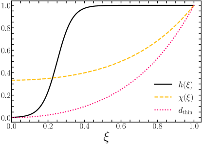
Figure 1: Comparison: $h(\xi)$, $\chi(\xi)$ (Minerbo closure) and $d_{\text{thin}}$. Logistic function with the parameters set in our tests: a transition at $\xi_{0}=1/3$ with a steepness $k=12$, such that the optically thick regime is fully recovered for $\xi\leq 0.1$ whereas for $\xi\geq 0.5$ the MC pressure tensor fully dominates the solution.

III.3 Matching the Moments: Lorentz Boost Link

We can modify $p_{k}^{a}$ to $\tilde{p}_{k}^{a}$ without changing its norm by using a Lorentz boost transformation that sends ${\cal{\bar{J}}}_{a}={\cal J}_{a}^{\texttt{MC}}$ into ${\cal J}_{a}={\cal J}_{a}^{\texttt{GM}}$. Since Lorentz transformations (defined as $\Lambda_{b}^{a}g^{bc}\Lambda_{c}^{d}=g^{ad}$) preserve vector norms, and ${\cal J}_{a}^{\texttt{MC}}$ is in general timelike and future-directed, for the desired transformation to exist, ${\cal J}_{a}^{\texttt{GM}}$ has to be timelike and future-directed as well. The explanation about why these vectors satisfy such properties can be found at the end of this subsection.

The Lorentz transformations connecting a given initial vector to a final one are referred to as Lorentz boost links. Several transformations addressing this problem can be found in the literature (see, for example, Oziewicz 2006; Celakoska et al. 2015). We have chosen the simplest option that fits our scheme, that is

$$\Lambda_{b}^{a}=\delta_{b}^{a}-\delta\Lambda_{b}^{a}~{},$$

where

$$\delta\Lambda_{b}^{a}=\frac{1}{-1+\frac{{\cal{\bar{J}}}_{d}{\cal{J}}^{d}}{{\cal{J}}{\cal{\bar{J}}}}}\left(\frac{{\cal{\bar{J}}}^{a}}{{\cal{\bar{J}}}}+\frac{{\cal{J}}^{a}}{{\cal{J}}}\right)\left(\frac{{\cal{\bar{J}}}^{b}}{{\cal{\bar{J}}}}+\frac{{\cal{J}}^{b}}{{\cal{J}}}\right)+\frac{2{\cal{J}}^{a}{\cal{\bar{J}}}_{b}}{{\cal{J}}\,{\cal{\bar{J}}}}~{},$$

being ${\cal{J}}=\sqrt{-{\cal{J}}_{d}{\cal{J}}^{d}}$ and ${\cal{\bar{J}}}=\sqrt{-{\cal{\bar{J}}}_{d}{\cal{\bar{J}}}^{d}}$ the norms of the respective moments.

We notice that this transformation is always well defined since, as we mentioned before, ${\cal{\bar{J}}}_{d}$ and ${\cal{J}}_{d}$ are timelike and future-directed. Therefore, $-1\leq\frac{{\cal{\bar{J}}}_{d}{\cal{J}}^{d}}{{\cal{J}}{\cal{\bar{J}}}}<0$, indicating that the denominators in the definition of $\delta\Lambda_{b}^{a}$ never go to zero.

This Lorentz boost link connects the two four-vectors as follows

$$\frac{{\cal{\bar{J}}}^{a}}{{\cal{\bar{J}}}}\Lambda_{a}^{b}=\frac{{\cal{J}}^{b}}{{\cal{J}}}.$$ (44)

We notice that, substituting Eq. (38) into this last expression, gives

$${\cal{J}}^{b}=\sum_{k\in\Delta V}\frac{{N}_{k}}{\sqrt{\gamma}\Delta V}\\ \left(\frac{{\cal{J}}}{{\cal{\bar{J}}}}{p_{k}}^{a}\Lambda_{a}^{b}\right),$$ (45)

which leads to the desired result

$${\cal{J}}^{b}=\sum_{k\in\Delta V}{N}_{k}\frac{\tilde{p}^{k}_{b}}{\sqrt{\gamma}\Delta V}~{}~{}\textup{with}~{}~{}\tilde{p}^{k}_{b}\equiv\frac{{\cal{J}}}{{\cal{\bar{J}}}}{p_{k}}^{a}\Lambda_{a}^{b}~{}.$$ (46)

The neutrino 4-momentum $\tilde{p}_{b}^{k}$ remains time-like (or null when $m_{\nu}=0$) due to the fact that the Lorentz transformation $\Lambda_{b}^{a}$ preserves the norm of $p_{a}^{k}$. In simpler terms, we have applied a boost/rotation to the neutrino 4-momentum of all the packets within a given cell, ensuring that the MC moments ($\bar{E},\bar{F}_{i}$) precisely match the corresponding GM moments in that specific cell.

Returning to the discussion on the norms of ${\cal J}_{a}^{\texttt{MC}}$ and ${\cal J}_{a}^{\texttt{GM}}$. Let us assume a tiny non-zero neutrino mass $m_{\nu}=\delta$, although negligible compared with the other scales in the problem. As indicated by Eq. (38), the direct consequence is that the 4-moment ${\cal J}_{a}^{\texttt{MC}}$ constitutes then a positive linear combination of future-directed timelike vectors . Consequently, ${\cal J}_{a}^{\texttt{MC}}$ must also be timelike and future-directed. To ensure the timelike and future-directed nature of ${\cal J}_{a}^{\texttt{M1}}$, we impose a consistency condition $F_{i}F^{i}\leq(1-\delta)E^{2}$ (see Levermore 1984). Finally, considering that ${\cal J}_{a}^{\texttt{GM}}$ (see Eq. (42)) is a positive linear combination of ${\cal J}_{a}^{\texttt{M1}}$ and ${\cal J}_{a}^{\texttt{MC}}$, we can conclude that it is also timelike and future-directed.

IV Numerical Tests

In this section we perform several stringent tests to validate our method and assess its accuracy. The numerical scheme employed for solving the M1 formalism was presented in detail in Izquierdo et al. (2023). In summary, the evolution equations are evolved in time by using an Implicit-Explicit Runge-Kutta (IMEX) time integrator, fourth order accurate for the explicit part and second order for the stiff terms. The spatial discretization is based on a High-Resolution Shock Capturing (HRSC) scheme with Finite Volume reconstruction, designed to be asymptotically preserving in the diffusion equation limit (Radice et al. 2022). The numerical scheme employed to solve the MC formalism has been elaborated upon throughout the manuscript, and it is predominantly inspired by the ones presented in (Foucart 2018; Foucart et al. 2021; Kawaguchi et al. 2023).

In the following we present the results of four distinct numerical solutions: M1 represents the uncoupled (i.e., stand-alone) truncated moment approach, MC denotes the uncoupled Monte-Carlo method, GM1 represents M1 solutions, using the GM formalism, and GMC designates MC solutions, using the GM formalism. These four solutions, each with its significant interest, will be subjected to thorough comparative analysis in the following numerical tests.

IV.1 Diffusion in a Moving Medium Test

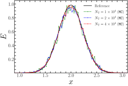
Figure 2: Diffusion in a Moving Medium Test. The profile of the energy density, reconstructed from the MC numerical solution, is displayed at time $t=4$ for different total number of packets $N_{\text{T}}$ by keeping the spatial resolution $\Delta x=0.02$ fixed. As $N_{\text{T}}$ increases, the numerical solution tends to the semi-analytic (reference) one.

Diffusion in a moving medium is a challenging test, considered also in (Radice et al. 2022; Izquierdo et al. 2023; Musolino and Rezzolla 2023; Cheong et al. 2023), which encapsulates most of the essential elements of the M1 implementation. The test consists on a pulse of radiation energy density, characterized by a Gaussian profile, propagating within a moving medium which is dominated by scattering dynamics (i.e., a high value of the scattering opacity $\kappa_{s}$). The complete dynamics can be accurately captured only with the correct treatment of stiff source terms.

The initial conditions at $t=0$ are specified as follows: $E(\mathbf{x})=e^{-9x^{2}}$, $v^{x}(\mathbf{x})=0.5$, $\kappa_{s}(\mathbf{x})=10^{3}$ and $\kappa_{a}(\mathbf{x})=\eta(\mathbf{x})=0$. The radiation fluxes, $F_{i}$, are initialized under the assumption that the radiation is fully trapped (i.e., $H^{a}=0$). Using the relations between frames, this condition translates into

$$J=\frac{3E}{4W^{2}-1}\,,\quad~{}~{}~{}~{}~{}F_{i}=\frac{4}{3}JW^{2}v_{i}\,.$$ (47)

In order to check the convergence of the numerical solutions we have considered three different spatial resolutions, corresponding to $\Delta x=(0.01,0.02,0.04$). For the evolution of the distribution function we have considered different fixed total number of packets $N_{\text{T}}=(0.5,1,2,4)\times 10^{4}$.

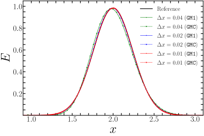
Figure 3: Diffusion in a Moving Medium Test. Comparison between the numerical solutions GM1 and GMC and the semi-analytic solution for several grid resolutions $\Delta x$ with a number of packets $N_{\text{T}}=2\times 10^{4}$ fixed. As $\Delta x$ decreases, the numerical solution tends to the semi-analytic (reference) one.

Fig. 2 illustrates the radiation energy density profile at time $t=4$, reconstructed from the MC solution, for various total numbers of packets $N_{\text{T}}=(1,2,4)\times 10^{4}$. The semi-analytic solution is also plotted for comparison purposes. A large number of packets has been employed to demonstrate that, as expected, with “infinite” resolution (i.e., $N_{\text{T}}\rightarrow\infty$), the MC formalism converges to the true solution. However, the number of packets required for an accurate MC solution in high-scattering regions is unfeasible in realistic scenarios of neutron star mergers.

This limitation is addressed by the GM scheme. In Fig. 3, the numerical solutions of GM1 and GMC are plotted for different spatial resolutions $\Delta x=(0.01,0.02,0.04$), keeping $N_{\text{T}}=2\times 10^{4}$ fixed. As the entire domain of this test is optically thick, we expect an almost exact matching of the lowest moments from M1 to MC with our choice of the function $h(\xi)$ (see Eq. (43) and Fig. 1). Consequently, GM1 and GMC are anticipated to precisely follow the M1 behavior (for a comparison between the M1 solution and the semi-analytic solution we refer to Izquierdo et al. 2023). Indeed, as it is shown in Fig. 3, both GM1 and GMC match perfectly the M1 solution, approaching the semi-analytic one as the resolution increases. It is worth noting that, in such optically thick regimes, the MC method tends to be computationally slow and usually provides a poor solution. Therefore, by choosing $h(\xi)$ as specified, we can ensure that our GM method remains as accurate and efficient as the M1 in this regime.

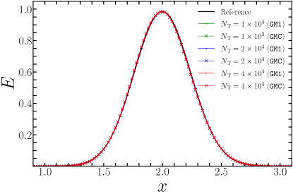
Figure 4: Diffusion in a Moving Medium Test. Comparison between the numerical solutions GM1 and GMC and the semi-analytic solution for various values of the total number of packets $N_{\text{T}}$ with a grid resolution $\Delta x=0.02$ fixed. The observed perfect matching shows that the GM solutions do not depend on the total number of packets in optically thick regimes.

These results are confirmed in Fig. 4, where the radiation energy density of the two GM numerical solutions is displayed by varying the total numbers of packets $N_{\text{T}}=(1,2,4)\times 10^{4}$ but keeping the spatial resolution $\Delta x=0.02$ fixed. As anticipated, both GM solutions remains unchanged, overlapping almost exactly with the semi-analytical one. Consequently, within the GM scheme, increasing the number of packets is not necessary to enhance the numerical solution in optically thick regions.

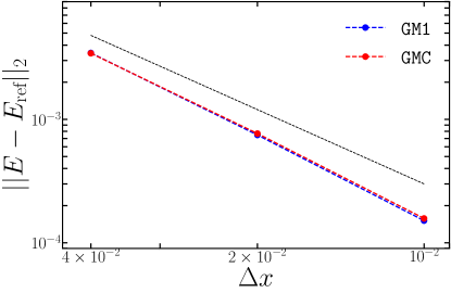
Figure 5: Diffusion in a Moving Medium Test. Convergence of the GM1 and GMC solutions to the reference solution for a fixed number of total packets $N_{\text{T}}=2\times 10^{4}$ by varying the grid resolution. We find an approximate second order convergence (dashed black line) for both GM1 and GMC solutions.

A more quantitative analysis of the observed results can be obtained by performing suitable convergence tests of the error, which can be defined as the (norm of the) difference between the numerical and the semi-analytical solution. Two types of convergence can be examined: either varying the total numbers of packets while keeping the grid resolution fixed, or varying the grid resolution while keeping the total number of packets fixed. The latter one is represented in Fig. 5 for a fixed number of total packets $N_{\text{T}}=2\times 10^{4}$. In this case, we find the expected second order of convergence of the M1 scheme, as reported in Izquierdo et al. (2023). As mentioned earlier, both the GM1 and GMC solutions closely follow the M1 solution. There exists a very small difference in the error between the GM1 and the GMC, originated by few cells which contain no packets and where the matching of the moments could not be performed.

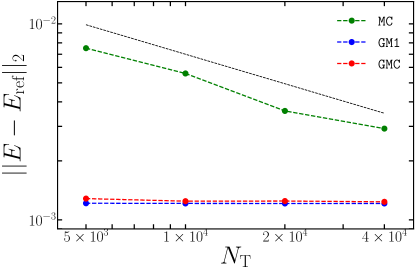
Figure 6: Diffusion in a Moving Medium Test. Convergence of the GM1 and GMC solutions to the reference solution for a fixed grid resolution $\Delta x=0.02$ by varying the number of total packets. We find the expected $N_{\text{T}}^{-1/2}$ convergence for the MC solution (dashed black line), but no dependence on $N_{\text{T}}$ for either the GM1 or the GMC solution.

The convergence keeping a fixed grid resolution $\Delta x=0.02$ is displayed in Fig. 6. Here, we find the anticipated MC convergence of $N_{\text{T}}^{-1/2}$. However, the error for both GM1 and GMC is much smaller and exhibit no improvement when increasing the total number of packets. This lack of improvement is attributed to the accuracy dominance of M1 over MC in the numerical solution for this test.

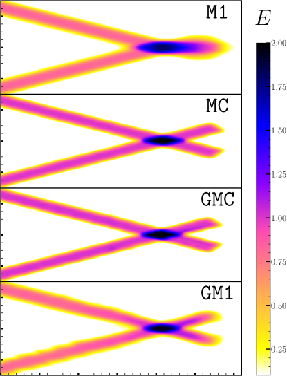
Figure 7: Double Beam Test. Numerical solutions for the (M1, MC, GMC, GM1) schemes are presented at the final time $t=0.5$, using $\Delta x=0.01$ and $N_{\text{T}}=5\times 10^{6}$ fixed. The behavior of M1 reveals a breakdown in the optically thin limit when multiple sources are present. In contrast, the (MC, GMC, GM1) solutions preserve the initial directions of the beams, enabling them to cross without interacting.

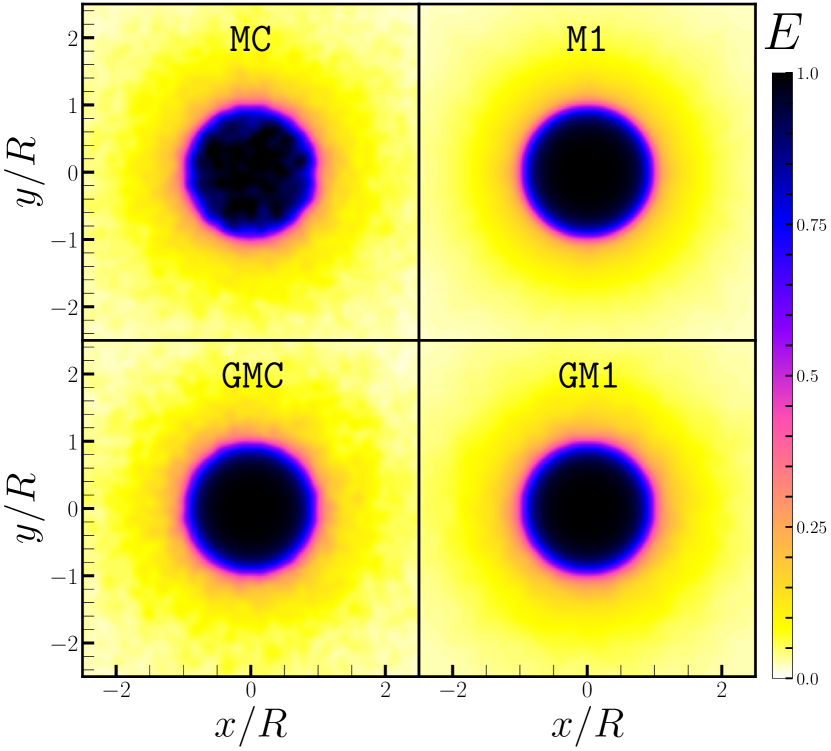
Figure 8: Radiating and Absorbing Sphere Test. The energy density, computed with the (MC, M1, GMC, GM1) schemes using $\Delta x=0.03$ and $N_{\text{tr}}=80$, is displayed at the equatorial plane at time $t=5$, when the solution has reached a steady state.

IV.2 Double Beam Test

This benchmark highlights the spectacular failure of the M1 formalism in optically thin regions when multiple sources are present (see, e.g., McKinney et al. 2014; Foucart et al. 2015; Weih et al. 2020b). In this two dimensional test, two radiation beams are injected into the domain. If we consider the radiation to be neutrinos, one would expect the beams to follow straight paths, crossing without interaction. However, the M1 scheme, treating radiation as a fluid, encounters challenges in this scenario since the closure is local and can only capture the physical behavior for a single source. On the other hand, the MC approach has no difficulties to find the correct physical solution.

In particular, we set the following initial conditions. We inject two beams of neutrinos from the left boundaries of the domain $(x,y)\in[-2,2]\times[-4.5,4.5]$ with an angle of $60^{\circ}$ degrees between them. In this test we consider only a relatively high-resolution case, with a fixed spatial grid resolution $\Delta x=0.01$ and total number of packets $N_{\text{T}}=5\times 10^{6}$. The simulation is performed with the four schemes (M1, MC, GMC, GM1) until the final time $t=0.5$, capturing the moment at which the beams have already intersected and continue along their trajectory.

The solutions of the energy density at this final time are presented in Fig. 7. As it was already mentioned, when two (or more) beams are present, the closure for the second moment in the M1 formalism lacks sufficient information, causing the two beams to merge into a single one propagating along the average of the original directions. Notice that, although the distribution function contains all the information about possible directions of propagation, the M1 formalism retains only a single averaged direction: momenta in opposite directions cancel each other out, resulting in a loss of information regarding the original momentum distribution (Weih et al. 2020b). In principle, the lost information could potentially be recovered by employing higher moments. In clear contrast, in the MC scheme the two beams intersect seamlessly without losing energy density or modifying their trajectories. A similar outcome, though not as pristine, is observed for the GMC and GM1 numerical solutions. This outcome highlights a significant advantage of our GM formalism, which demonstrates an accurate handling of the solution in optically thin regions.

IV.3 Radiating and Absorbing Sphere Test

A more challenging problem, which includes both the optically thick and thin regimes, is given by an a homogeneous radiating and absorbing sphere. This test, whose analytical solution is known, has been widely discussed in astrophysical literature (see, e.g., Smit et al. 1997; Pons et al. 2000; Rampp and Janka 2002; Radice et al. 2013b; Anninos and Fragile 2020, Weih et al. 2020b, Chan and Müller 2020b; Radice et al. 2022; Izquierdo et al. 2023; Musolino and Rezzolla 2023; Cheong et al. 2023), since it can be interpreted as a highly simplified model for an isolated, radiating neutron star.

The main configuration involves a static (i.e., $v^{i}(\mathbf{x})=0$), spherically symmetric, homogeneous sphere of radius $R$ with a constant energy density. In this idealized case, the only neutrino-matter interaction process allowed is the isotropic thermal absorption and emission.

$$\kappa_{a}(\mathbf{x},\mathbf{y},\mathbf{z}) =\eta(\mathbf{x},\mathbf{y},\mathbf{z})=\begin{cases}10&\text{for }r\leq R~{},\\ 0&\text{for }r>R~{},\end{cases}$$ (48)

$$\kappa_{s}(\mathbf{x},\mathbf{y},\mathbf{z}) =\mathbf{0}~{}.$$

where $r=\sqrt{x^{2}+y^{2}+z^{2}}$ and we have chosen $R=0.5$. Our 3D computational Cartesian domain is a cube of dimensions $[-2,2]^{3}$, discretized with different spatial grid resolution resolutions $\Delta x=(0.03,0.06,0.12)$. In this specific scenario, characterized by a non-zero emissivity, the simulation cost of the Monte-Carlo scheme is governed by the free parameter $N_{\text{tr}}$, related to the neutrino packets generated in a grid cell (see Eq. (30)). In this test, we have explored various values of $N_{\text{tr}}=(20,40,80)$.

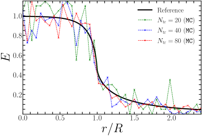
Figure 9: Radiating and Absorbing Sphere Test. Comparison between the MC numerical and the exact solutions for various values of the number of packets $N_{\text{tr}}$ with a fixed spatial resolution $\Delta x=0.03$. The statistical noise of the numerical solution decreases as the number of packets increases.

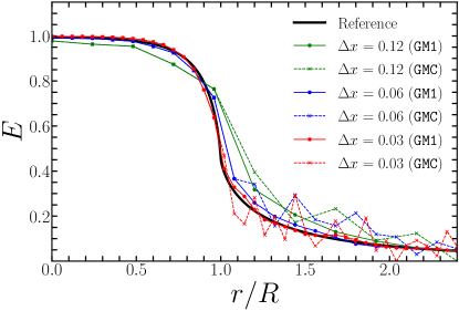
Figure 10: Radiating and Absorbing Sphere Test. Comparison between the numerical solutions GM1 and GMC and the analytic solution for various grid resolutions with a fixed number of packets $N_{\text{tr}}=40$. The GM1 clearly converges to the exact solution. However, in the case of GMC, while there is clearly convergence in the interior of the star, the presence of statistical noise remains fairly consistent over all grid resolutions.

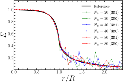
Figure 11: Radiating and Absorbing Sphere Test. Comparison between the numerical solutions for GM1 and GMC and the analytic one for various values of the number of packets while keeping a fixed grid resolution $\Delta x=0.03$. As in Fig. 9, the statistical noise decreases for both numerical solutions as the number of packets increases.

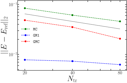
Figure 12: Radiating and Absorbing Sphere Test. Convergence of the (MC, GM1, GMC) solutions for a fixed grid resolution $\Delta x=0.03$ by varying the number of packets. We find the expected $N_{\text{T}}^{-1/2}$ convergence (dashed black line) of the MC method except for the GM1 solution, which presents already a very small error.

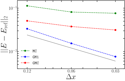
Figure 13: Radiating and Absorbing Sphere Test. Convergence of the (MC, GM1, GMC) solutions for a fixed number of packets $N_{\text{tr}}=40$ while varying the grid resolutions. We find an approximate first order convergence (dashed black line) for the GM1 but only a moderate improvement for the MC or GMC solutions, which only converge as the number of packets increases.

Fig. 8 displays the radiation energy density in the equatorial plane of the four considered schemes (MC, M1, GMC, GM1) at time $t=5$, when the solution has reached a steady state. These results, obtained using $\Delta x=0.03$ and $N_{\text{tr}}=80$, are consistent with our theoretical expectations. All methods produce a qualitative similar solution, with MC and GMC showing oscillations throughout the domain due to statistical noise (i.e., which would diminish with a greater number of packets), while the M1 and GM1 exhibit much smoother profiles. In particular, the GMC effectively resolves accurately the interior of the sphere, where we observe a full matching from the M1 solution onto the MC one, as expected in optically thick regions. In the exterior of the sphere, some oscillations appear due to the stochastic nature of the MC method, which is dominant in the optically thin region. The GM1 solution matches the M1 in the interior of the sphere, and it smoother than the GMC in the exterior. This positive outcome confirms that the GM approach retains the advantages of evolving a truncated moment scheme while incorporating new features that allow to handle accurately also the optically thin limit.

In order to assess quantitatively the accuracy of our methods, the radial profile of the energy density is compared against the analytical (reference) solution. The MC solution is presented in Fig. 9 for various numbers of packets corresponding to $N_{\text{tr}}=(20,40,80)$, while keeping the spatial resolution $\Delta x=0.03$ fixed. The inherent statistical noise of the MC is evident for all points in the domain, yet the solution progressively converges to the analytic one as the number of packets is increased. This test highlights one of the limitations of the MC scheme, namely its lower convergence rate. On the other hand, the solution of the M1 formalism displays a second order convergence when appropriate numerical schemes are employed (we refer to Izquierdo et al. 2023 for details).

We now turn on the results of our GM formalism. In Fig. 10, we compare the numerical solutions of GM1 and GMC with the analytic solution for different spatial resolutions $\Delta x=(0.03,0.06,0.12)$, while keeping the number of total packets approximately constant setting $N_{\text{tr}}=40$. Given the optically thick regime found in the star’s interior, the GMC solution exhibits no statistical noise in this region, unlike the outer region where oscillations are present. Interestingly, these oscillations are mostly suppresed in the GM1 solution. The average nature of the truncated moments formalism and the HRSC schemes employed for the evolution of the moments are probably the cause of this suppresion. Finally, notice that the GM1 solution converges to the analytical one as the grid spacing decreases. However, the GMC solution only converges clearly in the interior of the sphere. Outside there remains a statistical noise that does not depend on the grid resolution. In Fig. 11, we compare the numerical solutions of GM1 and GMC versus the analytic solution for different choices of the number of packets $N_{\text{tr}}=(20,40,80)$ keeping the spatial resolution $\Delta x=0.03$ fixed. As expected, the statistical noise outside the sphere is reduced as the number of packets increases.

Convergence tests are performed by varying the number of total packets while keeping the spatial resolution fixed and vice versa. The results of the former analysis are presented in Fig. 12, where the error in the numerical solution is displayed as a function of the total number of packets for a fixed spatial resolution $\Delta x=0.03$. Notably, the GM1 solution exhibits minimal improvement with increasing number of packets, given the dominance of the M1 solution in the interior, which already has negligible error, and the smoothness of the solution in the exterior. On the other hand, both GMC and MC demonstrates an approximate $1/2$ convergence, attributed to the suppression of statistical noise in the exterior of the star as the total number of packets increases. The convergence of the solutions as a function of the spatial grid resolution while keeping a fixed number of packets $N_{\text{tr}}=40$ is displayed in Fig. 13. Here, the GM1 solution shows a first-order convergence, while the MC and GMC solutions displays only a marginal improvement. This moderate improvement is mainly due to the projection of the M1 solution inside the star, while the solution in the exterior is still dominated by statistical noise which only decreases by increasing the number of packets. This result confirms that the GM formalism only converges to the exact solution for infinite grid resolution and infinite number of packets.

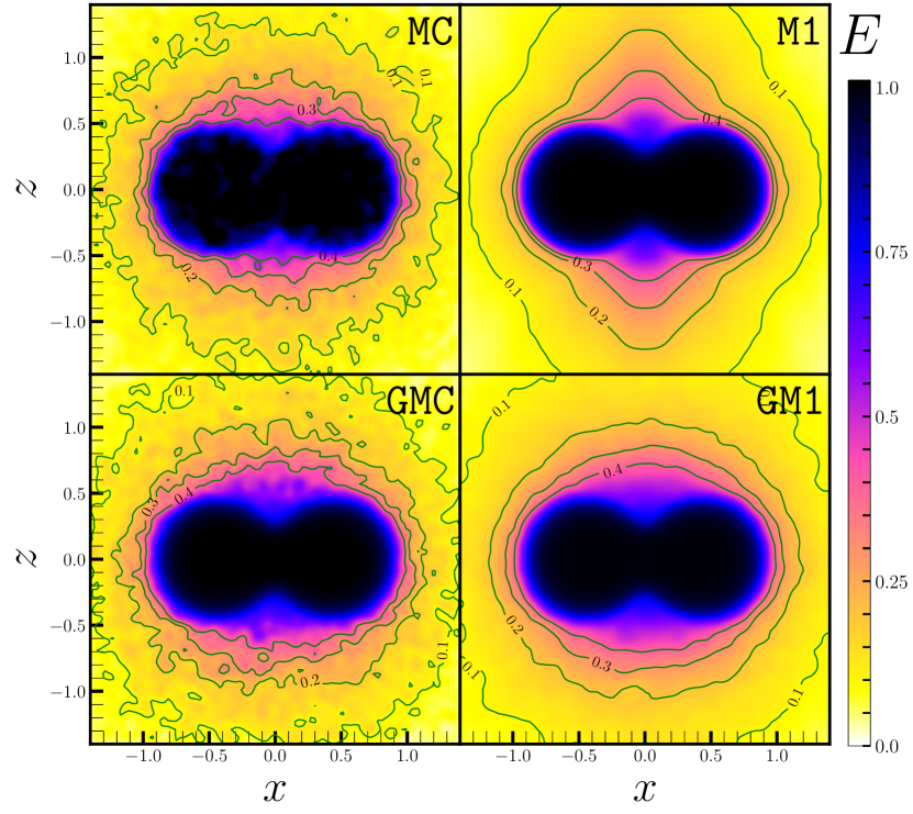
Figure 14: Radiating and Absorbing Torus Test. The energy density, computed with the (MC, M1, GMC, GM1) schemes using $\Delta x=0.03$ and $N_{\text{tr}}=40$, is displayed at the meridional plane at time $t=5$, when the solution has reached a steady state.

IV.4 Radiating and Absorbing Torus Test

In our last 3D problem we simulate a scenario reminiscent of the one discussed in Sec. IV.2, but without so many symmetries. The astrophysical motivation behind this configuration is to reproduce a simple model of the remnant resulting from a neutron star merger. Instead of an absorbing and radiating sphere, the geometry of the system is better approximated by a torus, which can be described by the following parametric equations in Cartesian coordinates:

$$x(u,v) =(R+r\cos v)\cos u~{},$$

$$y(u,v) =(R+r\cos v)\sin u~{},$$

$$z(u,v) =r\sin v~{}.$$

The coordinate position on the torus is determined by the parameters $(u,v)\in[0,2\pi)$, while that the major and minor radius $(R,r)$ define the type of torus. For our specific configuration, we have chosen a self-intersecting spindle torus (i.e., $r>R$) with $r=0.5$ and $R=0.45$ . Inside the torus, we set again high emissivity and absorption opacity $\eta=\kappa_{a}=10$, such that neutrinos in this region are in equilibrium with the fluid, representing the optically thick regime. Outside the torus, both the emissivity and absorption opacity are set to zero $\eta=\kappa_{a}=0$, modeling an optically thin medium. As the simulation begins, neutrinos emitted from the interior propagate to the exterior . Due to the geometry of the self-intersecting spindle torus, beams will collide along the symmetry axis (i.e., along the $z=0$ axis), resembling the collision of multiple beams of radiation. The simulation is performed in a 3D Cartesian cubic domain with dimensions $[-3,3]^{3}$, employing a fixed spatial resolution $\Delta x=0.03$ and number of packets $N_{\text{tr}}=40$.

In Fig. 14 we present the final time $t=5$, when the system has reached a steady state, for the four schemes considered (MC, M1, GMC, GM1). The plot displays a 2D slice along the meridional direction (i.e., $y=0$ plane). Similar to the previous test (Sec. IV.3), the MC solution appears less smooth due to its intrinsic statistical noise. The crucial distinction between the exact methods and the M1 becomes evident when looking along the $z$-axis. In the M1, a shock forms where beams collide, representing the previously discussed failure of this approach in the optically thin limit. On the other hand, in the cases of (MC, GM1, GMC), the solutions do not have a large-energy-density region along this axis caused by the artificial collision of radiation. Crucially, our GM formalism, particularly the GM1 solution, exhibits a solution with smoothness comparable to that of the M1, but without the presence of shocks. This result confirms and validates the accuracy of the GM method both in the optically thick and thin regimes.

V Conclusions

Modeling accurately the intricate physical scenarios within neutron star mergers, especially during the post-merger phase, demands sophisticated numerical simulations. Neutrinos, being crucial contributors to the dynamics and thermodynamics of these events, require a specialized treatment. Here we have introduced a novel approach, the Guided Moments (GM) formalism, to achieve an accurate and efficient full-neutrino transport treatment in complex environments like neutron star mergers and core-collapse supernovae. This formalism efficiently combines the advantages of the truncated moments scheme (M1) and Monte-Carlo (MC) based methods, providing a robust solution that addresses the strengths and weaknesses of each method.

One of the key concepts in the GM formalism is to compute the closure of the M1 evolution equations (i.e., the second moment) by using information from the MC solution. In the optically thick limit, this closure is analytical and provides already a very accurate and efficient solution. In the same regime, however, the MC scheme has an opposite behavior and faces with two challenges: the continuous emission and absorption of neutrino packets and the always present statistical noise associated to stochastic processes. To mitigate these issues, in our GM scheme, we use information from the M1 solution to modify the neutrino distribution function such that the MC lowest moments matches the ones evolved by the M1 formalism. On the other hand, the M1 closure in the optically thin limit is not known for multiple sources, so here our GM formalism takes advantage of the cost-effectiveness of the MC scheme to compute the exact closure in this regime.

These previous points and the deep discussion included in this paper, allow us to say that the GM formalism not only accurately captures the optically thick limit through the exact M1 closure, but also effectively resolves the optically thin limit, a known challenge for the M1 approach but accurately handled by MC methods. The resulting scheme outperforms both the M1 and MC approaches, providing a comprehensive and accurate solution in both regimes. Although we have focused on the pressure tensor closure, our method likely also improves the energy closure. Studying this issue is beyond the scope of the paper, but it will be thoroughly discussed in future work involving astrophysical scenarios.

The detailed exposition of the GM formalism, its formulation, and implementation, along with a thorough comparison against M1 and MC methods across various test problems, demonstrates the efficacy of the proposed approach. The computational cost of evolving the MC solution in optically thick regions can be substantial in real simulations. This issue can be mitigated within the GM scheme by effectively limiting the emissivities and opacities only in MC scheme for these regions, thereby reducing the overall computational cost. As there is a complete matching of the lowest moments of M1 and those of MC, there should not be any degradation of the accuracy in the GM solution.

Another potential improvement is related to modifying the matching function $h(\xi)$ (see Eq. (43) and Fig. 1), which determines the regime in which we will match the lowest moments calculated with the M1 solution with those obtained from the MC scheme. While the presented test problems show promising behavior, fine-tuning might be necessary in more realistic simulations and probably will require a more careful exploration.

Appendix A Matching the neutrino number density

Recent extensions of the M1 formalism (see, e.g., Foucart et al. 2016; Radice et al. 2022; Izquierdo et al. 2023) also evolve the number density of neutrinos. Notice that, without evolving the number density, the M1 formalism with the grey approximation does not conserve accurately the lepton number (Foucart et al. 2016). Although this issue might be not so dramatic in the GM approach, where there is a better estimate of the neutrino energy spectrum, it might still be problematic. To this aim, for each neutrino species one can introduce a neutrino number current $N^{a}$ following a conservation equation

$$\nabla_{a}N^{a}=\sqrt{-g}{\cal C}=\sqrt{-g}(\eta^{0}-\kappa_{a}^{0}n)~{},$$ (49)

where $n=-N^{a}u_{a}$ is the neutrino density in the fluid frame and $(\kappa_{a}^{0},\eta^{0})$ are the neutrino number absorption and emission coefficients, also to be computed from the fluid state and the information in the EoS tables.

Assuming that the neutrino number density and the radiation flux are aligned, this equation can be written in the $3+1$ decomposition as

$$\partial_{t}(\sqrt{\gamma}{N}) + \partial_{k}\left[\sqrt{\gamma}\left(-W\beta^{k}+\alpha Wv^{k}+\alpha\frac{H^{k}}{J}\right)\frac{{N}}{\Gamma}\right]=\alpha\sqrt{\gamma}\left(\eta^{0}-\kappa_{a}^{0}\frac{N}{\Gamma}\right)~{},$$ (50)

where $N=-n_{a}N^{a}=n\Gamma$ is the neutrino density in the inertial frame and

$$\Gamma=W-\frac{1}{J}H^{a}n_{a}=W\left(\frac{E-F_{a}v^{a}}{J}\right)~{}.$$ (51)

Within this new equation, one can estimate dynamically the average energy of the neutrinos $\epsilon_{\nu}$, since in the fluid frame the relation $J\approx n<\epsilon_{\nu}>$ is approximately satistied.

In the guided moments formalism we are matching the lowest moments, but it might be desirable also to match the neutrino number density if it is being evolved also in the M1.

It is straightforward to show that, in the discrete packet distribution, the neutrino number density and the lowest moments, measured in the grid frame, can be computed just as

$${\bar{N}}=\sum_{k\in\Delta V}\frac{N_{k}}{\sqrt{\gamma}\Delta V}~{},~{}~{}~{}{\cal{\bar{J}}}_{a}=\sum_{k\in\Delta V}N_{k}\frac{p^{k}_{a}}{\sqrt{\gamma}\Delta V}~{}.$$ (52)

The first step is to match the density of neutrino number ${\bar{N}}$ to $N$, a task that requires a modification of the weights $N_{k}$. This can be achieved by performing the following simple renormalization:

$$\tilde{N}_{k}\equiv\frac{N}{{\bar{N}}}N_{k}\rightarrow N=\sum_{k\in\Delta V}\frac{\tilde{N}_{k}}{\sqrt{\gamma}\Delta V}~{},$$ (53)

which imply that the projection of the stress-energy tensor needs to be computed now as

$${\cal{\bar{J}}}_{a}=\sum_{k\in\Delta V}{\tilde{N}}_{k}\frac{p^{k}_{a}}{\sqrt{\gamma}\Delta V}~{}.$$ (54)

Basically, the interpretation of this new relation for the moments is that by changing the number of neutrinos in a cell, automatically the energy and flux densities change in that cell.

The rest of the procedure for matching moments remains the same, such that the final result

$${\cal{J}}^{b}=\sum_{k\in\Delta V}{\tilde{N}}_{k}\frac{\tilde{p}^{k}_{b}}{\sqrt{\gamma}\Delta V}~{},$$ (55)

involves now two transformations: changing $N_{k}\rightarrow\tilde{N}_{k}$ (i.e., modifying the weights such that the density of neutrinos are equal) and $p^{k}_{b}\rightarrow\tilde{p}^{k}_{b}$ (i.e., modifying the neutrino 4-momentum such that the lowest moments match).

Appendix B Tetrad

Two special observers will play an important role in the description of our neutrino transport algorithm: inertial observers, whose timeline is tangent to $n^{a}$, and co-moving observers, whose timeline is tangent to $u^{a}$.

Our numerical grid is discretized in the spatial coordinates $x^{i}$. We will refer to the coordinates $(t,x^{i})$ as the inertial or grid frame, where the line element is

$$ds^{2}=g_{ab}dx^{a}dx^{b}~{}.$$ (56)

We also define the coordinates of the fluid rest frame $(t^{\prime},x^{i^{\prime}})$, which are defined at a point such that

$$ds^{2}=\eta_{a^{\prime}b^{\prime}}dx^{a^{\prime}}dx^{b^{\prime}}~{},$$ (57)

with $\eta_{a^{\prime}b^{\prime}}$ the Minkowski metric, and $(t^{\prime})^{a}=u^{a}$. We construct these local coordinates from an orthonormal tetrad $e^{(c^{\prime})}_{a}$, with

$$\hat{e}^{a}_{(t^{\prime})} = u^{a}~{},$$ (58)

$$g^{ab}\hat{e}_{a}^{(c^{\prime})}\hat{e}_{b}^{(d^{\prime})} = \eta^{c^{\prime}d^{\prime}}~{}.$$ (59)

The three other components of the tetrad are obtained by applying Gramm-Schmidt’s algorithm to the three vectors $V^{a}_{(i)}=\delta^{a}_{i}$ (i = 1, 2, 3). The orthonormal tetrad $\hat{e}_{(c^{\prime})}^{a}$, and the corresponding one-forms $\hat{e}^{(c^{\prime})}_{a}$, are precomputed and stored for each grid cell at each timestep, and can be used to easily perform transformations from the fluid rest frame coordinates to grid coordinates (and vice-versa) by simple matrix-vector multiplication.

In order to convert the 4-momentum from the lab frame ($\mathcal{S}$) to the fluid-rest-frame or comoving frame ($\mathcal{S^{\prime}}$) we need to find a basis that relates $p^{c}$ and $p^{c^{\prime}}$. This will be necessary when initializing the packets (set random moments), after scattering (redraw momentum) and when packets are emitted (new initialization). In these simulations, the momentum is draw in an spherical uniform distribution, i.e.,

$$p^{c^{\prime}}=\nu(1,\sin\theta\cos\phi,\sin\theta\sin\phi,\cos\theta)~{}.$$ (60)

We draw $\cos(\theta)$ from a uniform distribution in $[-1,1]$ and $\phi$ from a uniform distribution in $[0,2\pi]$. The 4-momentum of neutrinos in grid coordinates can then be computed using the transformation

$$p^{t} = \hat{e}^{t}_{(c^{\prime})}p^{c^{\prime}}~{},$$ (61)

$$p_{i} = g_{ia}\hat{e}^{a}_{(c^{\prime})}p^{c^{\prime}}=\delta_{c^{\prime}d^{\prime}}\hat{e}^{(c^{\prime})}_{i}p^{d^{\prime}}~{}.$$ (62)

References

- Abbott et al. (2017a) B. P. Abbott, R. Abbott, T. D. Abbott, F. Acernese, K. Ackley, C. Adams, T. Adams, P. Addesso, R. X. Adhikari, V. B. Adya, C. Affeldt, M. Afrough, B. Agarwal, M. Agathos, K. Agatsuma, and N. Aggarwal, The Astrophysical Journal Letters 848, L12 (2017a).
- Abbott et al. (2017b) B. P. Abbott et al. (LIGO Scientific Collaboration and Virgo Collaboration), Phys. Rev. Lett. 119, 161101 (2017b).
- Colombo et al. (2022) A. Colombo, O. S. Salafia, F. Gabrielli, G. Ghirlanda, B. Giacomazzo, A. Perego, and M. Colpi, The Astrophysical Journal 937, 79 (2022).
- Kiuchi et al. (2018) K. Kiuchi, K. Kyutoku, Y. Sekiguchi, and M. Shibata, Phys. Rev. D 97, 124039 (2018).
- Foucart (2023) F. Foucart, Living Reviews in Computational Astrophysics 9, 1 (2023).
- Lippuner and Roberts (2015) J. Lippuner and L. F. Roberts, The Astrophysical Journal 815, 82 (2015).
- Just et al. (2015a) O. Just, A. Bauswein, R. A. Pulpillo, S. Goriely, and H.-T. Janka, Monthly Notices of the Royal Astronomical Society 448, 541–567 (2015a).
- Thielemann et al. (2017) F.-K. Thielemann, M. Eichler, I. Panov, and B. Wehmeyer, Annual Review of Nuclear and Particle Science 67, 253–274 (2017).
- Perego et al. (2020) A. Perego, F. K. Thielemann, and G. Cescutti, “r-process nucleosynthesis from compact binary mergers,” in Handbook of Gravitational Wave Astronomy (Springer Singapore, Singapore, 2020) pp. 1–56.
- Dessart et al. (2008) L. Dessart, C. D. Ott, A. Burrows, S. Rosswog, and E. Livne, The Astrophysical Journal 690, 1681–1705 (2008).
- Perego et al. (2014) A. Perego, S. Rosswog, R. M. Cabezon, O. Korobkin, R. Kappeli, A. Arcones, and M. Liebendorfer, Monthly Notices of the Royal Astronomical Society 443, 3134–3156 (2014).
- Fujibayashi et al. (2017) S. Fujibayashi, Y. Sekiguchi, K. Kiuchi, and M. Shibata, The Astrophysical Journal 846, 114 (2017).
- Fujibayashi et al. (2020) S. Fujibayashi, S. Wanajo, K. Kiuchi, K. Kyutoku, Y. Sekiguchi, and M. Shibata, The Astrophysical Journal 901, 122 (2020).
- Foucart et al. (2022) F. Foucart, P. Laguna, G. Lovelace, D. Radice, and H. Witek, arXiv e-prints , arXiv:2203.08139 (2022), arXiv:2203.08139 [gr-qc] .
- Abdikamalov et al. (2012) E. Abdikamalov, A. Burrows, C. D. Ott, F. Löffler, E. O’Connor, J. C. Dolence, and E. Schnetter, The Astrophysical Journal 755, 111 (2012).
- Richers et al. (2015) S. Richers, D. Kasen, E. O’Connor, R. Fernández, and C. D. Ott, The Astrophysical Journal 813, 38 (2015).
- Ryan et al. (2015) B. R. Ryan, J. C. Dolence, and C. F. Gammie, “bhlight: General relativistic radiation magnetohydrodynamics with monte carlo transport,” (2015), arXiv:1505.05119 [astro-ph.HE] .
- Foucart (2018) F. Foucart, Monthly Notices of the Royal Astronomical Society 475, 4186 (2018).
- Foucart et al. (2018) F. Foucart, M. D. Duez, L. E. Kidder, R. Nguyen, H. P. Pfeiffer, and M. A. Scheel, Phys. Rev. D 98, 063007 (2018), arXiv:1806.02349 [astro-ph.HE] .
- Ryan and Dolence (2020) B. R. Ryan and J. C. Dolence, The Astrophysical Journal 891, 118 (2020).
- Foucart et al. (2021) F. Foucart, M. D. Duez, F. Hébert, L. E. Kidder, P. Kovarik, H. P. Pfeiffer, and M. A. Scheel, The Astrophysical Journal 920, 82 (2021).
- Kawaguchi et al. (2023) K. Kawaguchi, S. Fujibayashi, and M. Shibata, Physical Review D 107 (2023), 10.1103/physrevd.107.023026.
- Foucart et al. (2023) F. Foucart, M. D. Duez, R. Haas, L. E. Kidder, H. P. Pfeiffer, M. A. Scheel, and E. Spira-Savett, Physical Review D 107 (2023), 10.1103/physrevd.107.103055.
- Weih et al. (2020a) L. R. Weih, A. Gabbana, D. Simeoni, L. Rezzolla, S. Succi, and R. Tripiccione, Monthly Notices of the Royal Astronomical Society 498, 3374 (2020a), https://academic.oup.com/mnras/article-pdf/498/3/3374/33779378/staa2575.pdf .
- Pomraning (1973) G. Pomraning, The Equations of Radiation Hydrodynamics, International Series of Monographs in Natural Philosophy (Pergamon Press, Oxford, UK, 1973).
- McClarren and Hauck (2010) R. G. McClarren and C. D. Hauck, Journal of Computational Physics 229, 5597 (2010).
- Radice et al. (2013a) D. Radice, E. Abdikamalov, L. Rezzolla, and C. D. Ott, Journal of Computational Physics 242, 648 (2013a).
- Pomraning (1969) G. C. Pomraning, Journal of Quantitative Spectroscopy and Radiative Transfer 9, 407 (1969).
- Mihalas and Weibel-Mihalas (1999) D. Mihalas and B. Weibel-Mihalas, Foundations of Radiation Hydrodynamics (Dover Publications, Mineola, NY, USA, 1999).
- Chan and Müller (2020a) C. Chan and B. Müller, Monthly Notices of the Royal Astronomical Society 496, 2000–2020 (2020a).
- Bhattacharyya and Radice (2023) M. K. Bhattacharyya and D. Radice, Journal of Computational Physics 491, 112365 (2023).
- Fleck and Cummings (1971) J. Fleck and J. Cummings, Journal of Computational Physics 8, 313 (1971).
- Fleck and Canfield (1984) J. Fleck and E. Canfield, Journal of Computational Physics 54, 508 (1984).
- Wollaber (2008) A. B. Wollaber, Advanced Monte Carlo methods for thermal radiation transport, Ph.D. thesis, University of Michigan (2008).
- Richers et al. (2017) S. Richers, H. Nagakura, C. D. Ott, J. Dolence, K. Sumiyoshi, and S. Yamada, The Astrophysical Journal 847, 133 (2017).
- Ruffert et al. (1996) M. Ruffert, H. T. Janka, and G. Schaefer, A&A 311, 532 (1996), arXiv:astro-ph/9509006 [astro-ph] .
- Rosswog and Liebendörfer (2003) S. Rosswog and M. Liebendörfer, MNRAS 342, 673 (2003), arXiv:astro-ph/0302301 [astro-ph] .
- Sekiguchi (2010) Y. Sekiguchi, Classical and Quantum Gravity 27, 114107 (2010).
- Neilsen et al. (2014) D. Neilsen, S. L. Liebling, M. Anderson, L. Lehner, E. O’Connor, and C. Palenzuela, Phys. Rev. D 89, 104029 (2014).
- Palenzuela et al. (2015) C. Palenzuela, S. L. Liebling, D. Neilsen, L. Lehner, O. L. Caballero, E. O’Connor, and M. Anderson, Phys. Rev. D 92, 044045 (2015).
- Perego et al. (2016) A. Perego, R. M. Cabezón, and R. Käppeli, The Astrophysical Journal Supplement Series 223, 22 (2016).
- Most et al. (2019) E. R. Most, L. J. Papenfort, and L. Rezzolla, Monthly Notices of the Royal Astronomical Society 490, 3588 (2019), https://academic.oup.com/mnras/article-pdf/490/3/3588/30338124/stz2809.pdf .
- Palenzuela et al. (2022) C. Palenzuela, S. Liebling, and B. Miñano, Physical Review D 105 (2022), 10.1103/physrevd.105.103020.
- Thorne (1981) K. S. Thorne, MNRAS 194, 439 (1981).
- Shibata et al. (2011) M. Shibata, K. Kiuchi, Y. Sekiguchi, and Y. Suwa, Progress of Theoretical Physics 125, 1255 (2011), arXiv:1104.3937 [astro-ph.HE] .
- Sadowski et al. (2013) A. Sadowski, R. Narayan, A. Tchekhovskoy, and Y. Zhu, Monthly Notices of the Royal Astronomical Society 429, 3533 (2013), https://academic.oup.com/mnras/article-pdf/429/4/3533/3355151/sts632.pdf .
- McKinney et al. (2014) J. C. McKinney, A. Tchekhovskoy, A. Sadowski, and R. Narayan, Monthly Notices of the Royal Astronomical Society 441, 3177 (2014).
- Wanajo et al. (2014) S. Wanajo, Y. Sekiguchi, N. Nishimura, K. Kiuchi, K. Kyutoku, and M. Shibata, The Astrophysical Journal Letters 789, L39 (2014).
- Foucart et al. (2015) F. Foucart, E. O’Connor, L. Roberts, M. D. Duez, R. Haas, L. E. Kidder, C. D. Ott, H. P. Pfeiffer, M. A. Scheel, and B. Szilagyi, Physical Review D 91 (2015), 10.1103/physrevd.91.124021.
- Just et al. (2015b) O. Just, M. Obergaulinger, and H.-T. Janka, Monthly Notices of the Royal Astronomical Society 453, 3387 (2015b).
- Sekiguchi et al. (2015) Y. Sekiguchi, K. Kiuchi, K. Kyutoku, and M. Shibata, Physical Review D 91 (2015), 10.1103/physrevd.91.064059.
- Kuroda et al. (2016) T. Kuroda, T. Takiwaki, and K. Kotake, Astrophys. J. Suppl. 222, 20 (2016), arXiv:1501.06330 [astro-ph.HE] .
- Foucart et al. (2016) F. Foucart, E. O’Connor, L. Roberts, L. E. Kidder, H. P. Pfeiffer, and M. A. Scheel, Physical Review D 94 (2016), 10.1103/physrevd.94.123016.
- Skinner et al. (2019) M. A. Skinner, J. C. Dolence, A. Burrows, D. Radice, and D. Vartanyan, The Astrophysical Journal Supplement Series 241, 7 (2019).
- Fuksman and Mignone (2019) J. D. M. Fuksman and A. Mignone, The Astrophysical Journal Supplement Series 242, 20 (2019).
- Weih et al. (2020b) L. R. Weih, H. Olivares, and L. Rezzolla, Monthly Notices of the Royal Astronomical Society 495, 2285 (2020b).
- Radice et al. (2022) D. Radice, S. Bernuzzi, A. , and R. Haas, Monthly Notices of the Royal Astronomical Society 512, 1499 (2022).
- Izquierdo et al. (2023) M. R. Izquierdo, L. Pareschi, B. Miñano, J. Massó, and C. Palenzuela, Classical and Quantum Gravity 40, 145014 (2023).
- Cheong et al. (2023) P. C.-K. Cheong, H. H.-Y. Ng, A. T.-L. Lam, and T. G. F. Li, The Astrophysical Journal Supplement Series 267, 38 (2023).
- Musolino and Rezzolla (2023) C. Musolino and L. Rezzolla, “A practical guide to a moment approach for neutrino transport in numerical relativity,” (2023), arXiv:2304.09168 [gr-qc] .
- Schianchi et al. (2023) F. Schianchi, H. Gieg, V. Nedora, A. Neuweiler, M. Ujevic, M. Bulla, and T. Dietrich, arXiv e-prints , arXiv:2307.04572 (2023), arXiv:2307.04572 [gr-qc] .
- Ascher et al. (1997) U. M. Ascher, S. J. Ruuth, and R. J. Spiteri, Applied Numerical Mathematics 25, 151 (1997), special Issue on Time Integration.
- Pareschi and Russo (2000) L. Pareschi and G. Russo, “Implicit-explicit runge-kutta schemes for stiff systems of differential equations,” in Recent Trends in Numerical Analysis (Nova Science Publishers, Inc., USA, 2000) p. 269–288.
- Kennedy and Carpenter (2003) C. A. Kennedy and M. H. Carpenter, Applied Numerical Mathematics 44, 139 (2003).
- Pareschi and Russo (2005) L. Pareschi and G. Russo, Journal of Scientific Computing 25, 129 (2005).
- Degond et al. (2011) P. Degond, G. Dimarco, and L. Pareschi, International Journal for Numerical Methods in Fluids 67, 189 (2011), https://onlinelibrary.wiley.com/doi/pdf/10.1002/fld.2345 .
- Dimarco (2013) G. Dimarco, Kinetic and Related Models 6, 291 (2013).
- Levermore and Pomraning (1981) C. D. Levermore and G. C. Pomraning, ApJ 248, 321 (1981).
- Minerbo (1979) G. Minerbo, Computer Graphics and Image Processing 10, 48 (1979).
- Murchikova et al. (2017) E. M. Murchikova, E. Abdikamalov, and T. Urbatsch, Monthly Notices of the Royal Astronomical Society 469, 1725 (2017).
- Oziewicz (2006) Z. Oziewicz, arXiv preprint math-ph/0608062 (2006).
- Celakoska et al. (2015) E. Celakoska, D. Chakmakov, and M. Petrushevski, International Journal of Contemporary Mathematical Sciences 10, 85 (2015).
- Levermore (1984) C. D. Levermore, Journal of Quantitative Spectroscopy and Radiative Transfer 31, 149 (1984).
- Smit et al. (1997) J. M. Smit, J. Cernohorsky, and C. P. Dullemond, A&A 325, 203 (1997).
- Pons et al. (2000) J. A. Pons, J. M. Ibanez, and J. A. Miralles, Monthly Notices of the Royal Astronomical Society 317, 550 (2000).
- Rampp and Janka (2002) M. Rampp and H. T. Janka, Astron. Astrophys. 396, 361 (2002), arXiv:astro-ph/0203101 .
- Radice et al. (2013b) D. Radice, E. Abdikamalov, L. Rezzolla, and C. D. Ott, Journal of Computational Physics 242, 648 (2013b).
- Anninos and Fragile (2020) P. Anninos and P. C. Fragile, The Astrophysical Journal 900, 71 (2020).
- Chan and Müller (2020b) C. Chan and B. Müller, Monthly Notices of the Royal Astronomical Society 496, 2000 (2020b).