The EBLM Project XII. An eccentric, long-period eclipsing binary with a companion near the hydrogen-burning limit

Abstract

In the hunt for Earth-like exoplanets it is crucial to have reliable host star parameters, as they have a direct impact on the accuracy and precision of the inferred parameters for any discovered exoplanet. For stars with masses between 0.35 and 0.5 ${\rm M_{\sun}}$ an unexplained radius inflation is observed relative to typical stellar models. However, for fully convective objects with a mass below 0.35 ${\rm M_{\sun}}$ it is not known whether this radius inflation is present as there are fewer objects with accurate measurements in this regime. Low-mass eclipsing binaries present a unique opportunity to determine empirical masses and radii for these low-mass stars. Here we report on such a star, EBLM J2114-39 B. We have used HARPS and FEROS radial-velocities and TESS photometry to perform a joint fit of the data, and produce one of the most precise estimates of a very low mass star’s parameters. Using a precise and accurate radius for the primary star using Gaia DR3 data, we determine J2114-39 to be a $M_{1}=0.987\pm 0.059$ ${\rm M_{\sun}}$ primary star hosting a fully convective secondary with mass $M_{2}~{}=~{}0.0986~{}\pm 0.0038~{}\,\mathrm{M_{\sun}}$, which lies in a poorly populated region of parameter space. With a radius $R_{2}=~{}0.1275~{}\pm 0.0020~{}\,\mathrm{R_{\sun}}$, similar to TRAPPIST-1, we see no significant evidence of radius inflation in this system when compared to stellar evolution models. We speculate that stellar models in the regime where radius inflation is observed might be affected by how convective overshooting is treated.

1 Introduction

The key to estimating any exoplanet’s physical properties is to first determine its host star’s parameters accurately. Typically, host star parameters are determined by finding the closest fit between the stellar observables and stellar models (such as Baraffe et al., 2015; Dotter et al., 2008; Fernandes et al., 2019). Thus, any biases or missing physics present in stellar models will lead to biased stellar and planetary parameter estimates. One issue of particular concern is the M-dwarf radius inflation problem where M-dwarfs with masses in the range $0.3$ to $0.5~{}\rm M_{\odot}$ appear to have radii a few percent larger than predicted by typical stellar models (Torres & Ribas, 2002; López-Morales, 2007; Feiden & Chaboyer, 2012). Additionally, M-dwarf effective temperatures appear to fall below predictions (Parsons et al., 2018). It has been claimed that these factors compensate for each other such that the luminosity of M-dwarfs is accurately predicted by stellar models (Torres, 2007), but recent results have cast doubt on this claim (Swanye et al., 2023).

Although M-dwarf stars are the most common type of star in our galaxy (Kroupa, 2001; Chabrier, 2003; Henry et al., 2006), they are not as well-studied as solar-type stars. The Detached Eclipsing Binary Catalogue (DEBCat) archive reports only one set of double-lined eclipsing binaries with either component below $0.2~{}\rm M_{\odot}$ (Southworth, 2015; Casewell et al., 2018), meaning that empirical mass-radius relations, determined from detached, double-lined, eclipsing binaries typically do not include fully convective M-dwarfs ($\leq 0.35~{}\rm M_{\odot}$; Torres et al., 2010; Moya et al., 2018). One of the main objectives of the EBLM project (Eclipsing Binaries - Low Mass; Triaud et al., 2013) is to measure accurate masses and radii for a sufficiently large sample of very low-mass M-dwarfs such that an empirical mass-radius-metallicity relation can be calibrated for the lower main-sequence.

Due to their low masses and low brightnesses, M-dwarf stars can be difficult to study. However, as an eclipsing secondary star they can be investigated using the same methods routinely implemented for exoplanets. For this reason, the EBLM project (Triaud et al., 2013) can address the low number of studied M-dwarfs and begin to fill the poorly populated region of parameter space in the mass-radius diagram for stars with masses $<0.35~{}\rm M_{\odot}$. Populating this space is of particular importance for the study of exoplanets as low-mass stars approaching the hydrogen burning limit are ideal candidates for the detection of temperate Earth-sized planets (Nutzman & Charbonneau, 2008; Rodler & López-Morales, 2014; Gillon et al., 2017; Triaud, 2021; Delrez et al., 2022).

Results from the EBLM survey have in the past shown that fully convective M-dwarf radii are correlated with their primary host star’s metallicity, with very little evidence for a radius inflation problem (von Boetticher et al., 2019). Radius inflation for high-mass M-dwarfs has been explained as the result of stellar magnetic activity whereby close-in binaries are synchronised, increasing the dynamo effect (e.g. Feiden & Chaboyer, 2013). If true, one expects a reduction of inflation with increasing orbital period, but results from the EBLM project show no relation between radius and orbital separation (von Boetticher et al., 2019; Swanye et al., 2023).

Here, we present a new system from the EBLM sample, EBLM J2114-39 (hereafter J2114-39). In the past, we published radial-velocities (RVs) modelled together with eclipses from ground-based telescopes (e.g. Triaud et al., 2013; von Boetticher et al., 2019). More recently, we combined radial-velocities with photometry from two satellites CHEOPS and TESS (Swayne et al., 2021; Sebastian et al., 2023; Swanye et al., 2023). From now on, we will publish the rest of the EBLM systems combining HARPS and/or SOPHIE radial-velocities (as well as any available supplementary data), with photometry from TESS. This is the first such paper in the series. In Section 2 we describe the observations collected. Section 3 details how we estimate parameters for the primary star, and the modelling of all data is in Section 4. Section 5 explains how we ensure we extract the most accurate parameters for the secondary star. We discuss the results and conclude in Section 6.

2 Observations

For our analysis of J2114-39 (other designations: TIC 159730525, 2MASS J21143061-3918506, Gaia DR3 6583420566747746176) we used photometric data collected by TESS (Transiting Exoplanet Survey Satellite; Ricker et al., 2014), alongside spectra from the HARPS (Mayor et al., 2003) and FEROS (Kaufer et al., 1999) instruments. This is a single lined binary (SB1) with an eclipsing M-dwarf on a $P=~{}44.92471~{}\pm 0.00025~{}\,\rm{\ day}$ period orbiting a G-type primary. The J2114-39 system is located at $\alpha=21^{h}14^{\prime}30.61^{\prime\prime}$ and $\delta=-39^{\circ}18^{\prime}50.6^{\prime\prime}$ on the sky with $V_{\rm mag}=11.1$. J2114-39 was not originally included in the EBLM catalogue (and is thus missing from Triaud et al., 2017) as it was identified as a likely long-period transiting gas giant, but FEROS observations quickly revealed the companion to be too massive and therefore non-planetary. The star was then added to our observing programme to be monitored by HARPS to seek circumbinary exoplanets in the context of the BEBOP survey (Binaries Escorted By Orbiting Planets; Martin et al., 2019; Standing et al., 2023).

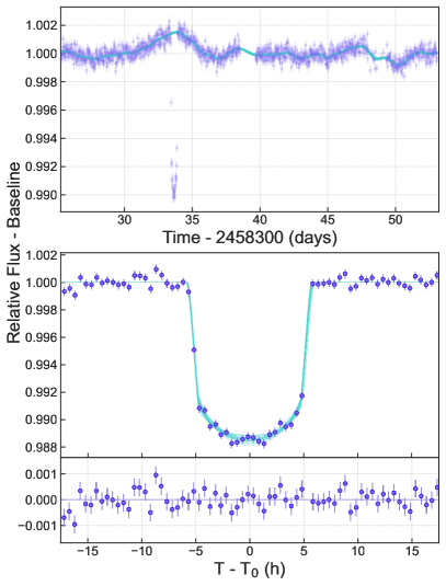
Figure 1: Top panel: Raw TESS data in purple with 20 random samples of the GP from the MCMC modelling the additional noise in blue. Middle panel: The phase-shifted eclipse of EBLM J2114-39, data shown in purple after the signal modelled by the GP has been removed. Twenty random samples from the MCMC run are displayed in teal colour. Bottom panel: The residuals to the best fit model.

The observations of J2114-39 with TESS were accessed using the Mikulski Archive for Space Telescopes (MAST) web service and downloaded using the lightkurve software package (Lightkurve Collaboration et al., 2018). The target was observed in Sector 1 where one eclipse is clearly present and Sector 28 which only contains out-of-eclipse data. The Sector 28 data is not included as it added no additional information to our fit. The phase-shifted lightcurve can be seen in Fig. 1. Due to the long orbital period compared to the $\sim$27 day TESS sector length, the secondary eclipse falls outside of the sectors observational windows. This analysis uses the 30-min cadence data products from the TESS-SPOC authors (Caldwell et al., 2020) which was processed with the Presearch Data Conditioning Simple Aperture Photometry (PDCSAP) algorithm (Stumpe et al., 2012; Smith et al., 2012) to remove systematic trends caused by instrumental noise.

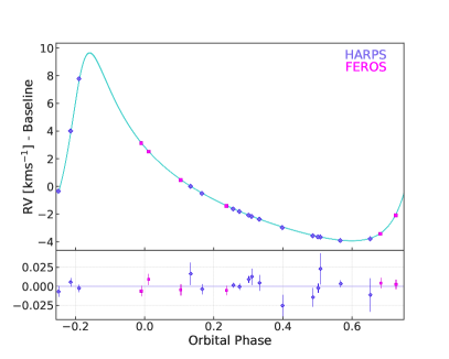
Figure 2: Phased radial-velocity measurements for EBLM J2114-39 from the HARPS (in purple) and FEROS (in pink) spectrographs. A sample of 20 random models from the MCMC are shown in teal colour. The residuals to best fit model are shown in the lower panel.

We have six recorded radial-velocity measurements of J2114-39 with FEROS, mounted on the 2.2m telescope at La Silla Observatory between 2019 Sep 12 and Nov 2019 Nov 28, and 16 radial-velocity measurements with the HARPS spectrograph, mounted on the ESO 3.6m telescope also at La Silla Observatory between 2020 Nov 18 and 2022 Nov 14. The FEROS observations were performed in the context of the Warm gIaNts with tEss collaboration (WINE, Hobson et al., 2021; Trifonov et al., 2023; Brahm et al., 2023). The radial velocities of the primary star measured from these spectra using cross-correlation against a numerical mask based on the solar spectrum are given in Tables 3 and 4 for the HARPS and FEROS observations respectively, and the phased radial-velocity curve can be seen in Fig. 2.

These six FEROS measurements were acquired with the simultaneous wavelength calibration technique where the second fibre is illuminated by the ThAr lamp to trace instrumental radial velocity drifts during the science exposure. We adopted an exposure time of 900 s, which produced spectra with a typical signal-to-noise ratio of 100 per resolution element. FEROS data were processed with the ceres (Brahm et al., 2017) pipeline, which generates optimally extracted, wavelength calibrated, and drift corrected spectra from the raw science images. Then we computed the radial velocities with the cross-correlation technique by using a G2 binary mask as template, where a gaussian is fitted to the cross-correlation peak.

The HARPS data were reduced by the standard (now public) data reduction software (DRS; Lovis & Pepe, 2007). After reduction, the spectra were cross-correlated with a G2 mask. The resulting cross-correlation function (CCF) is fitted with a Gaussian with its mean as the radial-velocity.

3 Spectroscopic Analysis and Stellar Properties

Atmospheric parameters for the primary star were obtained using the PAWS pipeline as part of the work completed in Freckelton et al. (2023) which is based on iSpec (Blanco-Cuaresma, 2019). One strength of PAWS is that effective temperature ($T_{\rm eff}$), surface gravity ($\log\,g_{1}$), metallicity ($\rm[Fe/H]$), microturbulent velocity ($v_{\rm mic}$), and project rotational velocity ($vsini_{\star}$) are fitted for, when other commonly used methods will keep at least one fixed. Within the pipeline, initial estimates of $T_{\rm eff}$, $\log\,g_{1}$, $\rm[Fe/H]$, and $v_{\rm mic}$ were generated using the curve-of-growth equivalent widths method with the WIDTH (Sbordone et al., 2004) radiative transfer code. PAWS then uses these as inputs to a spectral synthesis method, wherein free parameters are iterated until a synthesised spectrum based upon them matches the observed one. The synthetic spectra are generated using the SPECTRUM radiative transfer code (Gray & Corbally, 1994). $T_{\rm eff}$, $\log\,g_{1}$, $\rm[Fe/H]$, and $v_{\rm mic}$ were all set as free parameters during the analysis of J2114-39. Employment of the spectral synthesis method means we are also able to include macroturbulent velocity ($v_{\rm mac}$) and projected rotational velocity ($v\sin i_{1}$) as free parameters.

As part of the pipeline all spectra are shifted into the laboratory frame, and normalised to a continuum flux of 1.0. In order to produce the best results possible, the 16 HARPS spectra for J2114-39 were co-added to achieve a signal-to-noise ratio, $SNR=257$. The pipeline assumes solar-type parameters as an input to the equivalent widths method, using those outlined by Blanco-Cuaresma (2019). To ensure homogeneity throughout analysis, the SPECTRUM (Gray & Corbally, 1994) line list was used in both methods present in the pipeline, in addition to the ATLAS (Kurucz, 2005) set of model atmospheres.

The primary’s mass and radius are derived by interpolation of MIST isochrones (Dotter, 2016; Choi et al., 2016) based on the atmospheric parameters $\rm T_{\rm eff}$, $\rm[Fe/H]$, together with the parallax and infrared colours as input parameters and using a nested sampling approach implemented in the isochrones package (Morton, 2015). The stated uncertainty is the average of the errors calculated from the 16 and 84 percentiles of the resulting distribution. All values, taken from Freckelton et al. (2023) are reported in Table 2.

4 Global Modelling

To analyse the data from J2114-39 we use allesfitter (Günther & Daylan, 2021, 2019) to perform a simultaneous Markov Chain Monte Carlo (MCMC) modelling of the primary and secondary stars. allesfitter amalgamates many useful python packages frequently used in modelling stellar or planetary systems. At the heart of allesfitter is ellc (Maxted, 2016) which generates lightcurves and celerite (Foreman-Mackey et al., 2017) for any modelling with Gaussian processes (GPs). To obtain most likely parameters, two types of samplers are used; a nested sampler (dynesty; Speagle, 2020) and an affine-invariant MCMC sampler (emcee; Foreman-Mackey et al., 2013; Goodman & Weare, 2010). Here, as in other EBLM papers we use MCMC, since it is less computationally intensive and we have no requirement for model comparison. The nested sampling approach gives similar results to those from the MCMC. All results presented in the tables and in Section 6 are from a MCMC fit.

Orbital eccentricity, $e$, in allesfitter is reparameterised with respect to the argument of periastron, $\omega$, as $f_{\rm c}=\sqrt{e}\cos{\omega}$ and $f_{\rm s}=\sqrt{e}\sin{\omega}$ (as in Triaud et al., 2011). For limb darkening, we apply the quadratic law with $T_{\rm eff}$, $\log{g_{1}}$ and $\rm{[Fe/H]}$ as stellar properties, and adopt the output from PyLDTk (Parviainen & Aigrain, 2015) (using the PHOENIX stellar atmosphere library; Husser et al., 2013). Limb darkening coefficients are reparameterised to $q_{1}$ and $q_{2}$ following Kipping (2013) for the fitting process. All priors are described in Table 1.

From a visual inspection it is clear that there is a level of variability in the TESS photometry, likely caused by stellar activity. We first tried to apply polynomial and spline functions, but none returned a good fit. To account for intrinsic variability of the star and instrumental noise we fit a GP to the out-of-eclipse photometry assuming a Matérn $3/2$ kernel which detrends short and long term fluctuations. We fit for two hyper-parameters; the amplitude scale $\sigma$ and the length scale $\rho$, as required for this choice of kernel. For the radial-velocity data we add a jitter term (as part of $\ln\sigma_{\rm RV}$) in quadrature with the instrumental white noise error to account for any stellar variability effects, as well as normalised scaling parameters (included in $\ln{\sigma_{\mathrm{phot}}}$) for the photometry. Other parameters within the model include; the ratio of radii ($R_{2}/R_{1}$), inverse scaled semi-major axis ($(R_{1}+R_{2})/a$), cosine of the orbital inclination ($\cos i$), eclipse epoch ($T_{0}$), orbital period ($P$), radial-velocity semi-amplitude for the primary star ($K_{1}$), and constant baseline offsets for the radial-velocity instruments ($\Delta F_{\rm RV}$).

Prior to executing the MCMC sampling, we first perform a visual inspection of the photometric and spectroscopic data to ascertain suitable initial values and priors for the walkers such that the initial fit produces an acceptable and sensible result. When initial values are far from the solutions, walkers take significantly longer to converge, increasing the computational time needlessly for entirely comparable results. For similar reasons, we perform a short MCMC on the radial-velocity data only, before carrying out any joint sampling with the photometry. This allows for more informed estimates of the orbital period and eccentricity of the system. Once satisfied with the fit, the prior space is widened to ensure biases were not introduced to the fit by limiting its explorable parameter space.

For the final analysis the MCMC has 60 walkers with 30,000 steps, including 8000 burn-in steps which we discard. The final solutions, considered to be most probable, are determined by the median value of each fitted parameter’s posterior distribution where the quoted upper and lower estimates of uncertainty represent the 16/84 percentiles. We consider the chains to have converged to a solution as they were at least 100 times the autocorrelation length for each parameter as well as the chains visually converging in trial plots.

All fitted parameters included in the fit are presented in Table 1 alongside further details on the type of priors used and the selected bounds for the sampling. Physical parameters, derived from the fitted parameters are found in Table 2.

Table 1: Priors used in the fit and resulting output for the fitted parameters. Uniform priors are marked as $\mathcal{U}$(lower limit, upper limit) and normal priors marked as $\mathcal{N}$(mean, standard deviation). All times are given in $\rm BJD_{UTC}$. The quoted upper limits correspond to the 99.7 percentile of the posterior distribution.

	Parameter	Prior	Fit value & Uncertainty
Ratio of radii ;	$R_{2}/R_{1}$	$\mathcal{U}(0.080,0.12)$	$0.0997\pm 0.0008$
Inverse scaled semi-major axis ;	$(R_{1}+R_{2})/a$	$\mathcal{U}(0.020,0.035)$	$0.02570_{-0.00030}^{+0.00040}$
Orbital inclination ;	$\cos i$	$\mathcal{U}(0.00,0.02)$	$0.0026_{-0.0018}^{+0.0021}$
Eclipse epoch ;	$T_{0}$ (BJD)	$\mathcal{U}(2\,458\,333.62,2458333.72)$	$2\,458\,333.6695_{-0.0012}^{+0.0014}$
Orbital period ;	$P$ (days)	$\mathcal{U}(44.91,44.95)$	$44.92471\pm 0.00025$
Radial-velocity semi-amplitude ;	$K$ ($\rm{km}s^{-1}$)	$\mathcal{U}(6.0,7.0)$	$6.7870_{-0.0069}^{+0.0067}$
Eccentricity and argument of periastron transformation ;	$f\rm{{}_{c}}$	$\mathcal{U}(0.50,0.60)$	$0.55915\pm 0.00058$
Eccentricity and argument of periastron transformation ;	$f\rm{{}_{s}}$	$\mathcal{U}(-0.54,-0.44)$	$-0.50465\pm 0.00077$
Baselines per instrument
Matérn 3/2 hyperparameter, amplitude scale ;	$\ln\sigma$	$\mathcal{U}(-10.0,0.0)$	$-7.64_{-0.17}^{+0.21}$
Matérn 3/2 hyperparameter, length scale ;	$\ln\rho$	$\mathcal{U}(-5.0,5.0)$	$0.35_{-0.21}^{+0.23}$
Baseline offset HARPS ;	$\gamma_{\rm HARPS}$ ($\rm{km}s^{-1}$)	$\mathcal{U}(-25.5,-24.5)$	$-24.9828\pm 0.0036$
Baseline offset FEROS ;	$\gamma_{\rm FEROS}$ ($\rm{km}s^{-1}$)	$\mathcal{U}(-25.5,-24.5)$	$-24.9978\pm 0.0031$
Errors per instrument
Error scaling for TESS photometry	$\ln\sigma_{\rm TESS}$	$\mathcal{U}(-10.0,-7.0)$	$-7.979\pm 0.021$
HARPS jitter term ;	$\ln\sigma_{\rm HARPS}{(\rm km\,s^{-1})}$	$\mathcal{U}(-10.0,-2.0)$	$<-4.6\pm 1.6$
FEROS jitter term ;	$\ln\sigma_{\rm FEROS}{(\rm km\,s^{-1})}$	$\mathcal{U}(-10.0,-2.0)$	$<-3.9$
Limb Darkening Coefficients
Transformed limb darkening ;	$q_{\rm 1;TESS}$	$\mathcal{N}(0.1545856,0.5)$	$0.172_{-0.073}^{+0.11}$
Transformed limb darkening ;	$q_{\rm 2;TESS}$	$\mathcal{N}(0.520898,0.5)$	$0.47_{-0.20}^{+0.27}$

5 Parameter derivation

To extract accurate parameters on the secondary star, we need accurate parameters on the primary. Thanks to Gaia DR3 (Gaia Collaboration et al., 2016) the stellar radius ($R_{1}$) is better estimated than the mass ($M_{1}$) that traditionally relies on applying stellar models. However, thanks to our lightcurve modelling we can constrain $M_{1}$ using the stellar density. From Kepler’s law, stellar density ($\rho_{\rm 1}$) is defined as

$$\frac{M_{\rm 1}}{R_{\rm 1}^{3}}=\frac{4\pi^{2}}{G\,P^{2}}\left(\frac{a}{R_{\rm 1}}\right)^{3}-\frac{M_{\rm 2}}{R_{\rm 1}^{3}},$$ (1)

where $G$ is the gravitational constant, and $a$ is the semi-major axis (Triaud et al., 2013).

In planetary cases the second term ($M_{2}/R_{1}^{3}$) is typically considered negligible. However, for binary stars, it must be included, since its contribution is no longer insignificant. For eclipsing binaries we are able to determine the primary and secondary masses independent of any assumption of $M_{1}$.

We start by rearranging Eqn.1 for $M_{2}$ and define the total mass term as

$$M=\frac{4\pi^{2}}{G\,P^{2}}\left(\frac{a}{R_{\rm 1}}\right)^{3}R_{1}^{3}=M_{1}+M_{2}.$$ (2)

Then using the observables fit via the method described in Section 4 from each step in the MCMC we calculate the mass function, $f_{m}$ (Hilditch, 2001),

$$f_{m}=\frac{(1-e^{2})^{3/2}}{\sin^{3}{i}}\,\frac{P\,K_{1}^{3}}{2\pi\,G}.$$ (3)

As the mass function can also be expressed as

$$f_{m}=\frac{M_{\rm 2}^{3}}{(M_{\rm 1}+M_{\rm 2})^{2}}=C,$$ (4)

we can substitute in our expression from the stellar density equation to calculate a secondary mass

$$M_{2}=\sqrt[3]{CM^{2}}.$$ (5)

Finally with a value for $M_{2}$ we can now use Eqn.1 to calculate the primary mass as

$$M_{1}=M-M_{2}.$$ (6)

From the eclipse signal analysis, ${a}/{R_{\rm 1}}$ is a modelled variable along with all other observables in Eqn 1 and 3 which allows for the stellar masses to be calculated. To ensure the error in the the primary radius, $R_{1}$ (the only assumed value from outside the modelling), is reflected in the final mass uncertainty we assign a normal Gaussian distribution and draw random samples to be worked through in the same manner as all other variables.

6 Results and Conclusion

After the global modelling and parameter derivation, we determine a mass function $f_{m}=0.0008127\pm 0.0000028~{}\,\mathrm{M_{\sun}}$, indicating a low-mass companion. Then we calculate the secondary’s surface gravity $\log g_{2}=5.222\pm 0.0135$, which is found in absolute terms (Southworth et al., 2007) from parameters fit with the MCMC. This value alone confirms the secondary is a dense star, near the bottom of the main-sequence. Assuming parameters for the primary star (as in Section 3; $R_{1}=1.279\pm 0.017~{}\,\rm R_{\odot}$ and Section 5: $M_{1}=0.987\pm 0.059~{}\,\rm M_{\odot}$), we find the secondary stellar companion to be a late M-dwarf with a mass $M_{2}~{}=~{}0.0986~{}\pm 0.0038~{}\,\mathrm{M_{\sun}}$and a radius $R_{2}=~{}0.1275~{}\pm 0.0020~{}\,\mathrm{R_{\sun}}$and thus a mass ratio $q=0.0999\pm 0.0022$ with the primary. If we recalculate the surface gravity of the primary star using the obtained mass and radius, we find that the value is consistent within 1 sigma with the spectroscopic surface gravity, regardless of the choice of primary mass value. From the fit, we also find the system has a clearly detected orbital eccentricity $e=0.56767\pm 0.00045$, which is not unusual for a binary with this period (e.g. Triaud et al., 2017).

Without following the parameter derivationprocedure described in Section 5, we would have calculated the mass of the secondary star through equation 4 where we would have assumed the denominator to be $M_{1}^{2}$ as commonly done when $M_{2}\ll M_{1}$. By using the primary mass value calculated from isochrones, we would then have found the mass of the secondary companion to be $M_{2}=0.1038~{}\pm 0.0067~{}\,\rm M_{\odot}$ instead of $M_{2}~{}=~{}0.0986~{}\pm 0.0038~{}\,\mathrm{M_{\sun}}$. Although these results are consistent within error margins (as can be seen in Fig. 3) this represents a $\sim 5.0\%$ systematic bias towards higher masses (and would therefore bias the overall population towards less inflated objects). Appendix A details why the fractional uncertainty on mass is smaller for the secondary star than for the primary.

EBLM J2114-39b has a mass approaching the hydrogen burning limit, which is a key region for empirical calibrations of the mass-radius relation. As illustrated in the mass-radius plot (Fig. 3), our target is consistent within $1~{}\sigma$ with the Baraffe et al. (2015) models continuing a trend observed in von Boetticher et al. (2019) and Swanye et al. (2023), where fully convective secondary stars do not appear to be systematically inflated whereas higher mass M-dwarfs are. Several mechanisms have been proposed to explain radius inflation, however these explanations do not predict why fully convective stars would be different and not show inflation. Here we speculate that this might have to do with convective overshooting, which is known to affect modelled stellar parameters (e.g. Baraffe et al., 2023). For a fully convective star such as EBLM J2114-39 B, convective overshooting is essentially irrelevant since there is no penetration of convective materials into a radiative interior. However slightly more massive stars, with a small radiative core, might be very sensitive to how convective overshooting is modelled, since any plume of convective material into the small radiative interior would likely affect a greater fraction of the core, and might produce large differences in stellar evolution.

Another aspect that makes J2114-39B stand out in this context is its long orbital period. Typically other objects of a similar mass are found in binary systems with periods $<10~{}\rm\,days$. As such EBLM J2114-39B is likely not much influenced by its primary.

Table 2: Parameters of EBLM J2114-39. ^(∗) from Freckelton et al. (2023) and ^(∗∗) from GAIA DR3. Primary mass values given from the MIST isochrones $M_{1,\rm iso}$, as well as from the method described in Section 5. The quoted upper limits correspond to the 99.7 percentile of the posterior distribution.

Primary star parameters
Primary mass∗	$M_{1,\rm iso}$ ($\mathrm{M_{\odot}}$)	$1.038\pm 0.064$
Primary mass	$M_{1}$ ($\mathrm{M_{\odot}}$)	$0.987_{-0.060}^{+0.058}$
Primary radius∗	$R_{1}$ ($\rm R_{\odot}$)	$1.279\pm 0.017$
Effective temperature∗	$T_{\rm eff}$ (K)	$5763\pm 216$
Metallicity∗	[Fe/H] (dex)	$-0.03\pm 0.14$
Spectroscopic surface gravity∗	$\log g_{1}$ (cgs)	$4.241\pm 0.035$
Projected rotational velocity∗	$v\sin i_{1}$ ($\rm km\,s^{-1}$)	$1.60\pm 0.22$
Macroturbulent velocity∗	$v_{\rm mac}$ ($\rm km\,s^{-1}$)	$4.26\pm 1.37$
Microturbulent velocity∗	$v_{\rm mic}$ ($\rm km\,s^{-1}$)	$1.08\pm 0.22$
Parallax∗∗	Plx (mas)	$4.30\pm 0.02$
Secondary star derived parameters
Scaled primary radius	$R_{1}/a$	$0.02338_{-0.00028}^{+0.00036}$
Scaled secondary radius	$R_{2}/a$	$0.002329_{-0.000029}^{+0.000044}$
Orbital eccentricity	$e$	$0.56767_{-0.00043}^{+0.00046}$
Argument of periastron	$\omega$ (deg)	$317.933_{0.073}^{0.071}$
Secondary mass	$M_{2}$ ($\mathrm{M_{\odot}}$)	$0.0986_{-0.0039}^{+0.0037}$
Secondary radius	$R_{2}$ ($\rm R_{\odot}$)	$0.1275\pm 0.0020$
Mass Ratio	$q$	$0.0999_{-0.0020}^{+0.0023}$
Impact parameter	$b$	$<0.348$
Total eclipse duration	$T_{\mathrm{tot}}$ (h)	$11.624_{-0.097}^{+0.11}$
Full eclipse duration	$T_{\mathrm{full}}$ (h)	$9.469_{-0.097}^{+0.11}$
Eclipse depth	$\delta_{\mathrm{undil}}$	$0.01140_{-0.00015}^{+0.00016}$
Limb darkening	$u_{1}$	$0.39_{-0.11}^{+0.10}$
Limb darkening	$u_{2}$	$0.03_{-0.18}^{+0.21}$
Mass function	$f_{m}$ ($\rm M_{\odot}$)	$0.0008127\pm 0.0000028$
Companion surface gravity	$\log g_{2}$ (cgs)	$5.222_{-0.016}^{+0.011}$

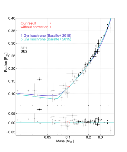
Figure 3: Mass-radius diagram with logarithmic mass axis, showing published single-lined systems (SB1) in grey, double-lined binaries (SB2) in black and EBLM J2114-39 in coral colour. The $1~{}\rm Gyr$ and $5~{}\rm Gyr$ isochrones are shown in purple and teal respectively. The lower panel highlights differences between the objects and the $5~{}\rm Gyr$ isochrone. Black and grey data points from compendium (and cited papers) in Triaud et al. (2020), with additional points from Morales et al. (2009).

Data Availability

All HARPS and FEROS data can be obtained from the ESO archive. All TESS data can be obtained from MAST.

Appendix A Error calculation for stellar masses

The fractional error on the secondary star is smaller than the fractional error on the primary mass. This may be surprising, but is actually a direct result of the fit to the RVs being very good and the different powers in the mass ratio of equation 4. From equation 5, we can write that

$$M_{2}^{3}=C\,M^{2}.$$

Using the rules of error propagation, we can show that

$$\left(\frac{\sigma_{M_{2}}}{M_{2}}\right)^{2}=\frac{4}{9}\left(\frac{\sigma_{M}}{M}\right)^{2}+\frac{1}{9}\left(\frac{\sigma_{C}}{C}\right)^{2}.$$

The error in $M$ can be calculated from equation 6:

$$\sigma_{M}^{2}=\sigma_{M_{1}}^{2}-\sigma_{M_{2}}^{2}$$

after which it follows that

$$\left(\frac{\sigma_{M_{2}}}{M_{2}}\right)^{2}=\frac{4}{9}\frac{\sigma_{M_{1}}^{2}-\sigma_{M_{2}}^{2}}{\left(M_{1}+M_{2}\right)^{2}}+\frac{1}{9}\left(\frac{\sigma_{C}}{C}\right)^{2}.$$

Rearranging this equation finally gives us

$$\left(\frac{\sigma_{M_{2}}}{M_{2}}\right)^{2}=\frac{4\,M_{1}^{2}}{9\,(M_{1}+M_{2})^{2}+4\,M_{2}^{2}}\left(\frac{\sigma_{M_{1}}}{M_{1}}\right)^{2}$$

$$\qquad\qquad+\frac{(M_{1}+M_{2})^{2}}{9\,(M_{1}+M_{2})^{2}+4\,M_{2}^{2}}\left(\frac{\sigma_{C}}{C}\right)^{2}$$

In the limiting case of a perfect fit to the RVs and thus $\sigma_{C}=0$, this reduces to

$$\left(\frac{\sigma_{M_{2}}}{M_{2}}\right)^{2}=\frac{4\,M_{1}^{2}}{9\,(M_{1}+M_{2})^{2}+4\,M_{2}^{2}}\left(\frac{\sigma_{M_{1}}}{M_{1}}\right)^{2}<\left(\frac{\sigma_{M_{1}}}{M_{1}}\right)^{2}$$

where it is now obvious that the precision on $M_{2}$ is better than the one on $M_{1}$. This will still hold for very good fits to the RVs where the fractional error in $C$ remains small, as is the case for our binary system. At some point, the error from the RV fit will be large enough that it is no longer the case, for example in the regime of planets orbiting stars where the RV fits are not as well constrained. We note that with a slight adjustment, it can also be shown that the secondary mass precision could also be better than the primary mass precision in the case of non-transiting binary systems where the primary mass comes from isochrone analysis. In that case $\sigma_{M}^{2}=\sigma_{M_{1}}^{2}+\sigma_{M_{2}}^{2}$.

Appendix B RV data

Table 3: HARPS observations of J2114-39. All times are given in $\rm BJD_{UTC}$.

BJD (day)	RV $(\rm kms^{-1})$	$\sigma$ $(\rm kms^{-1})$	Exposure Time (s)	SNR
2459171.599696	-28.74679	0.02187	300	6.7
2459425.784454	-27.12687	0.01073	300	10.6
2459433.716703	-28.52944	0.01232	300	9.5
2459462.782953	-24.95927	0.01488	300	8.5
2459479.607512	-28.61051	0.02043	300	6.1
2459516.622836	-27.34166	0.01040	300	11.7
2459519.599470	-27.93342	0.01410	300	8.7
2459535.500919	-25.31486	0.00703	300	15.4
2459703.926928	-28.60003	0.00585	300	18.1
2459737.860021	-26.58939	0.00350	900	27.9
2459761.691474	-20.98407	0.00583	900	18.3
2459823.663107	-25.47391	0.00667	900	16.7
2459828.499860	-26.78018	0.00444	900	24.1
2459841.604636	-28.86199	0.00446	900	23.2
2459874.628686	-27.04324	0.00460	900	23.3
2459897.565604	-17.22338	0.00511	900	21.3

Table 4: FEROS observations of J2114-39. All times are given in $\rm BJD_{UTC}$.

BJD (day)	RV $(\rm kms^{-1})$	$\sigma$ $(\rm kms^{-1})$	SNR
2458738.55034	-22.4797	0.0072	43.3
2458742.71029	-24.5180	0.0074	40.0
2458782.52082	-21.8770	0.0069	45.7
2458793.56281	-26.3889	0.0061	52.5
2458813.54052	-28.3868	0.0071	40.5
2458815.52633	-27.0573	0.0062	51.1

References

- Baraffe et al. (2015) Baraffe I., Homeier D., Allard F., Chabrier G., 2015, A&A, 577, A42
- Baraffe et al. (2023) Baraffe I., et al., 2023, MNRAS, 519, 5333
- Blanco-Cuaresma (2019) Blanco-Cuaresma S., 2019, MNRAS, 486, 2075
- Brahm et al. (2017) Brahm R., Jordán A., Espinoza N., 2017, PASP, 129, 034002
- Brahm et al. (2023) Brahm R., et al., 2023, AJ, 165, 227
- Caldwell et al. (2020) Caldwell D. A., et al., 2020, Research Notes of the American Astronomical Society, 4, 201
- Casewell et al. (2018) Casewell S. L., et al., 2018, MNRAS, 481, 1897
- Chabrier (2003) Chabrier G., 2003, PASP, 115, 763
- Choi et al. (2016) Choi J., Dotter A., Conroy C., Cantiello M., Paxton B., Johnson B. D., 2016, ApJ, 823, 102
- Delrez et al. (2022) Delrez L., et al., 2022, A&A, 667, A59
- Dotter (2016) Dotter A., 2016, ApJS, 222, 8
- Dotter et al. (2008) Dotter A., Chaboyer B., Jevremović D., Kostov V., Baron E., Ferguson J. W., 2008, ApJS, 178, 89
- Feiden & Chaboyer (2012) Feiden G. A., Chaboyer B., 2012, ApJ, 757, 42
- Feiden & Chaboyer (2013) Feiden G. A., Chaboyer B., 2013, ApJ, 779, 183
- Fernandes et al. (2019) Fernandes C. S., Van Grootel V., Salmon S. J. A. J., Aringer B., Burgasser A. J., Scuflaire R., Brassard P., Fontaine G., 2019, ApJ, 879, 94
- Foreman-Mackey et al. (2013) Foreman-Mackey D., Hogg D. W., Lang D., Goodman J., 2013, PASP, 125, 306
- Foreman-Mackey et al. (2017) Foreman-Mackey D., Agol E., Ambikasaran S., Angus R., 2017, AJ, 154, 220
- Freckelton et al. (2023) Freckelton A. V., Sebastian D., Mortier A., Triaud A., et a., 2023, submitted to MNRAS
- Gaia Collaboration et al. (2016) Gaia Collaboration et al., 2016, A&A, 595, A1
- Gillon et al. (2017) Gillon M., et al., 2017, Nature, 542, 456
- Goodman & Weare (2010) Goodman J., Weare J., 2010, Communications in Applied Mathematics and Computational Science, 5, 65
- Gray & Corbally (1994) Gray R. O., Corbally C. J., 1994, AJ, 107, 742
- Günther & Daylan (2019) Günther M. N., Daylan T., 2019, Allesfitter: Flexible Star and Exoplanet Inference From Photometry and Radial Velocity, Astrophysics Source Code Library (ascl:1903.003)
- Günther & Daylan (2021) Günther M. N., Daylan T., 2021, ApJS, 254, 13
- Henry et al. (2006) Henry T. J., Jao W.-C., Subasavage J. P., Beaulieu T. D., Ianna P. A., Costa E., Méndez R. A., 2006, AJ, 132, 2360
- Hilditch (2001) Hilditch R. W., 2001, An Introduction to Close Binary Stars
- Hobson et al. (2021) Hobson M. J., et al., 2021, AJ, 161, 235
- Husser et al. (2013) Husser T.-O., Wende-von Berg S., Dreizler S., Homeier D., Reiners A., Barman T., Hauschildt P. H., 2013, A&A, 553, A6
- Kaufer et al. (1999) Kaufer A., Stahl O., Tubbesing S., Nørregaard P., Avila G., Francois P., Pasquini L., Pizzella A., 1999, The Messenger, 95, 8
- Kipping (2013) Kipping D. M., 2013, MNRAS, 435, 2152
- Kroupa (2001) Kroupa P., 2001, MNRAS, 322, 231
- Kurucz (2005) Kurucz R. L., 2005, Memorie della Societa Astronomica Italiana Supplementi, 8, 14
- Lightkurve Collaboration et al. (2018) Lightkurve Collaboration et al., 2018, Lightkurve: Kepler and TESS time series analysis in Python, Astrophysics Source Code Library (ascl:1812.013)
- López-Morales (2007) López-Morales M., 2007, ApJ, 660, 732
- Lovis & Pepe (2007) Lovis C., Pepe F., 2007, A&A, 468, 1115
- Martin et al. (2019) Martin D. V., et al., 2019, A&A, 624, A68
- Maxted (2016) Maxted P. F. L., 2016, A&A, 591, A111
- Mayor et al. (2003) Mayor M., et al., 2003, The Messenger, 114, 20
- Morales et al. (2009) Morales J. C., et al., 2009, ApJ, 691, 1400
- Morton (2015) Morton T. D., 2015, isochrones: Stellar model grid package, Astrophysics Source Code Library, record ascl:1503.010 (ascl:1503.010)
- Moya et al. (2018) Moya A., Zuccarino F., Chaplin W. J., Davies G. R., 2018, ApJS, 237, 21
- Nutzman & Charbonneau (2008) Nutzman P., Charbonneau D., 2008, PASP, 120, 317
- Parsons et al. (2018) Parsons S. G., et al., 2018, MNRAS, 481, 1083
- Parviainen & Aigrain (2015) Parviainen H., Aigrain S., 2015, MNRAS, 453, 3821
- Ricker et al. (2014) Ricker G. R., et al., 2014, in Oschmann Jacobus M. J., Clampin M., Fazio G. G., MacEwen H. A., eds, Society of Photo-Optical Instrumentation Engineers (SPIE) Conference Series Vol. 9143, Space Telescopes and Instrumentation 2014: Optical, Infrared, and Millimeter Wave. p. 914320 (arXiv:1406.0151), doi:10.1117/12.2063489
- Rodler & López-Morales (2014) Rodler F., López-Morales M., 2014, ApJ, 781, 54
- Sbordone et al. (2004) Sbordone L., Bonifacio P., Castelli F., Kurucz R. L., 2004, Memorie della Societa Astronomica Italiana Supplementi, 5, 93
- Sebastian et al. (2023) Sebastian D., et al., 2023, MNRAS, 519, 3546
- Smith et al. (2012) Smith J. C., et al., 2012, PASP, 124, 1000
- Southworth (2015) Southworth J., 2015, in Rucinski S. M., Torres G., Zejda M., eds, Astronomical Society of the Pacific Conference Series Vol. 496, Living Together: Planets, Host Stars and Binaries. p. 164 (arXiv:1411.1219), doi:10.48550/arXiv.1411.1219
- Southworth et al. (2007) Southworth J., Wheatley P. J., Sams G., 2007, MNRAS, 379, L11
- Speagle (2020) Speagle J. S., 2020, MNRAS, 493, 3132
- Standing et al. (2023) Standing M. R., et al., 2023, Nature Astronomy, 7, 702
- Stumpe et al. (2012) Stumpe M. C., et al., 2012, PASP, 124, 985
- Swanye et al. (2023) Swanye M. I., Maxted P. F. L., et a., 2023, submitted to MNRAS
- Swayne et al. (2021) Swayne M. I., et al., 2021, MNRAS, 506, 306
- Torres (2007) Torres G., 2007, ApJ, 671, L65
- Torres & Ribas (2002) Torres G., Ribas I., 2002, ApJ, 567, 1140
- Torres et al. (2010) Torres G., Andersen J., Giménez A., 2010, A&ARv, 18, 67
- Triaud (2021) Triaud A. H. M. J., 2021, in Madhusudhan N., ed., , ExoFrontiers; Big Questions in Exoplanetary Science. pp 6–1, doi:10.1088/2514-3433/abfa8fch6
- Triaud et al. (2011) Triaud A. H. M. J., et al., 2011, A&A, 531, A24
- Triaud et al. (2013) Triaud A. H. M. J., et al., 2013, A&A, 549, A18
- Triaud et al. (2017) Triaud A. H. M. J., et al., 2017, A&A, 608, A129
- Triaud et al. (2020) Triaud A. H. M. J., et al., 2020, Nature Astronomy, 4, 650
- Trifonov et al. (2023) Trifonov T., et al., 2023, AJ, 165, 179
- von Boetticher et al. (2019) von Boetticher A., et al., 2019, A&A, 625, A150