Split-Ensemble: Efficient OOD-aware Ensemble via Task and Model Splitting

Abstract

Uncertainty estimation is crucial for machine learning models to detect out-of-distribution (OOD) inputs. However, the conventional discriminative deep learning classifiers produce uncalibrated closed-set predictions for OOD data. A more robust classifiers with the uncertainty estimation typically require a potentially unavailable OOD dataset for outlier exposure training, or a considerable amount of additional memory and compute to build ensemble models. In this work, we improve on uncertainty estimation without extra OOD data or additional inference costs using an alternative Split-Ensemble method. Specifically, we propose a novel subtask-splitting ensemble training objective, where a common multiclass classification task is split into several complementary subtasks. Then, each subtask’s training data can be considered as OOD to the other subtasks. Diverse submodels can therefore be trained on each subtask with OOD-aware objectives. The subtask-splitting objective enables us to share low-level features across submodels to avoid parameter and computational overheads. In particular, we build a tree-like Split-Ensemble architecture by performing iterative splitting and pruning from a shared backbone model, where each branch serves as a submodel corresponding to a subtask. This leads to improved accuracy and uncertainty estimation across submodels under a fixed ensemble computation budget. Empirical study with ResNet-18 backbone shows Split-Ensemble, without additional computation cost, improves accuracy over a single model by 0.8%, 1.8%, and 25.5% on CIFAR-10, CIFAR-100, and Tiny-ImageNet, respectively. OOD detection for the same backbone and in-distribution datasets surpasses a single model baseline by, correspondingly, 2.2%, 8.1%, and 29.6% mean AUROC. Codes will be publicly available at https://antonioo-c.github.io/projects/split-ensemble

1 Introduction

Deep learning models achieve high accuracy metrics when applied to in-distribution (ID) data. However, such models deployed in the real world can also face corrupted, perturbed, or out-of-distribution inputs (Hendrycks & Dietterich, 2019). Then, model predictions cannot be reliable due to uncalibrated outputs of the conventional softmax classifiers. Therefore, estimation of the epistemic uncertainty with OOD detection is crucial for trustworthy models (Gal & Ghahramani, 2016).

In general, uncertainty estimation is not a trivial task. Practitioners often consider various statistics derived from the uncalibrated outputs of softmax classifiers as confidence scores (Hendrycks et al., 2022). On the other hand, deep ensembling is another popular approach (Lakshminarayanan et al., 2017), where uncertainty can be derived from predictions of independently trained deep networks. However, deep ensembles come with large memory and computational costs, which grow linearly with the ensemble size. Recent research investigates strategies to share and reuse parameters and processing across ensemble submodels (Gal & Ghahramani, 2016; Wen et al., 2020; Turkoglu et al., 2022). Though these techniques reduce memory overheads, they suffer from the reduced submodel diversity and, thus, uncertainty calibration. Moreover, their computational costs remain similar to the naive deep ensemble since the inference through each individual submodel is still required.

More advanced methods for uncertainty estimation using a single model include temperature scaling, adversarial perturbation of inputs (Liang et al., 2017), and classifiers with the explicit OOD class trained by OOD-aware outlier exposure training (Hendrycks et al., 2018). However, as outlier exposure methods typically outperform other approaches that do not rely on external OOD-like data, OOD data distribution can be unknown or unavailable to implement effective outlier exposure training in practical applications.

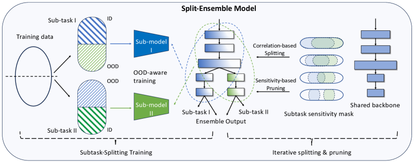
Figure 1: Overview. We split an original task into complementary subtasks to create objectives for subtask training. All submodels form an ensemble to perform the original task, and, importantly, each submodel can be trained with OOD-aware objectives of the subtask as proposed in Section 3. To implement an efficient Split-Ensemble architecture, we start with a shared backbone and iteratively perform splitting and pruning based on subtask sensitivity described in Section 4.

This work aims to propose novel training objectives and architectures to build a classifier with a single-model cost, without external OOD proxy data, while achieving ensemble-level performance and uncertainty estimation. To avoid the redundancy of having multiple ensemble submodels learn the same task, we, instead, split an original multiclass classification task into multiple complementary subtasks. As illustrated in Figure 1, each subtask is defined by considering a subset of classes in the original training data as ID classes. Then, the rest of the training set is a proxy for OOD distribution for the subtask. This enables our novel training objective with subtask splitting, where each submodel is trained with OOD-aware subtask objectives without external data. Finally, an ensemble of all submodels implements the original multiclass classification.

Our splitting objective requires a method to design computationally efficient submodel architectures for each subtask. Most subtasks processing, as part of the original task, can utilize similar low-level features. Hence, it is possible to share early layers across submodels. Moreover, as each subtask is easier than the original task, we can use lighter architectures for the latter unshared processing in submodels when compared to the backbone design of the original task. By considering these two observations, we propose a novel iterative splitting and pruning algorithm to learn a tree-like Split-Ensemble model. As illustrated in Figure 1, the Split-Ensemble shares early layers for all submodels. Then, they gradually branch out into different subgroups, and, finally, result in completely independent branches for each submodel towards the last layers. Global structural pruning is further performed on all the branches to remove redundancies in submodels. Given the potential large design space of Split-Ensemble architectures, we propose a correlation-based splitting and a pruning criteria based on the sensitivity of model weights to each subtask’s objective. This method enables automated architecture design through a single training run for our Split-Ensemble.

In summary, the paper makes the following contributions:

• We propose a subtask-splitting training objective to allow OOD-aware ensemble training without external data.

• We propose a dynamic splitting and pruning algorithm to build an efficient tree-like Split-Ensemble architecture to perform the subtask splitting.

• We empirically show that the proposed Split-Ensemble approach significantly improves accuracy and OOD detection over a single model baseline with a similar computational cost, and outperforms $4\times$ larger ensemble baselines.

In the rest of this paper, we discuss related work in Section 2, derive the subtask-splitting training objectives in Section 3, propose criteria and algorithm for splitting and pruning the architecture in Section 4, and show experiment results in Section 5.

2 Related work

2.1 OOD detection and OOD-aware training

OOD detection has a long history of research including methods applicable to deep neural networks (DNNs). Lane et al. (2007) firstly propose to use classification confidence scores to perform in-domain verification through a linear discriminant model. Liang et al. (2017) enhance OOD detection by temperature scaling and adversarial perturbations. Papadopoulos et al. (2021) propose a method for outlier exposure training with OOD proxy data without compromising ID classification accuracy. Zhou et al. (2020) investigate the differences between OOD-unaware/-aware DNNs in model performance, robustness, and uncertainty. Winkens et al. (2020) investigate the use of contrastive training to boost OOD detection performance. Jeong & Kim (2020) propose a few-shot learning method for detecting OOD samples. Besides supervised learning, Sehwag et al. (2021) investigate self-supervised OOD detector based on contrastive learning. Wang et al. (2022) propose partial and asymmetric supervised contrastive Learning (PASCL) to distinguish between tail-class ID samples and OOD samples. However, the above single-model OOD detectors cannot be implemented without the availability of OOD proxy data. Unlike this, our work proposes a novel subtask-splitting training objective to allow OOD-aware learning without external data.

2.2 Deep ensembles

Ensemble methods improve performance and uncertainty estimation by using predictions of multiple ensemble members, known as submodels. Lakshminarayanan et al. (2017) propose the foundational basis for estimating uncertainty in neural networks using ensemble techniques. However, computational and memory costs grow linearly with the number of submodels in deep ensembles. To improve efficiency, Havasi et al. (2021) replace single-input and single-output layers with multiple-input and multiple-output layers, Gal & Ghahramani (2016) extract model uncertainty using random dropouts, and Durasov et al. (2021) utilize fixed binary masks to specify network parameters to be dropped. Wen et al. (2020) enhance efficiency by expanding layer weights using low-rank matrices, and Turkoglu et al. (2022) adopt feature-wise linear modulation to instantiate submodels from a shared backbone. These methods aim to mitigate the parameter overheads associated with deep ensembles. However, they cannot reduce computational costs because each submodel runs independently. Split-Ensemble overcomes the redundancy of ensemble processing by having submodels that run complementary subtasks with layer sharing. In addition, we further optimize Split-Ensemble design with tree-like architecture by splitting and pruning steps.

2.3 Efficient multi-task learning

With the subtask splitting, our method also falls into the domain of multi-task learning. Given the expense of training individual models for each task, research has been conducted to train a single model for multiple similar tasks. Sharma et al. (2017) propose an efficient multi-task learning framework by simultaneously training multiple tasks. Ding et al. (2021) design Multiple-level Sparse Sharing Model (MSSM), which can learn features selectively with knowledge shared across tasks. Sun et al. (2021) introduce Task Switching Networks (TSNs), a task-conditioned architecture with a single unified encoder/decoder for efficient multi-task learning. Zhang et al. (2022) develop AutoMTL that automates efficient MTL model development for vision tasks. Sun et al. (2022) propose pruning algorithm on a shared backbone for multiple tasks. In this work, we explore correlations between multiple subtasks to design a novel splitting and pruning algorithm. Previous work of split-based structure search consider layer splitting (Wang et al., 2019; Wu et al., 2019; 2020) to increase the number of filters in certain layers for better model capacity. Split-Ensemble, on the other hand, uses architecture splitting as a way of deriving efficient architecture under a multi-task learning scenario of subtask-splitting training, leading to a novel tree-like architecture.

3 Subtask-splitting training

In this section, we provide the definition of subtask splitting given a full classification task in Section 3.1. We also derive proper training objective to improve both accuracy and uncertainty calibration for submodels learning these subtasks in Section 3.2, and how final classification and OOD detection is performed with the ensemble of subtask models in Section 3.3, as in Figure 2.

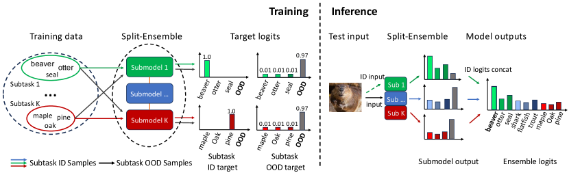
Figure 2: Subtask splitting. Each submodel learns its subtask using a subset of the original training data. OOD detection by outlier exposure training is realized using other subtasks’ examples. Concatenated ID logits from all submodels implement the original multiclass classification task.

3.1 Complementary subtask splitting

Consider a classification task with $N$ classes in total. In most large-scale real-world datasets, it is by design that some classes are semantically closer than others, and all classes can be grouped into multiple semantically-close groups (e.g. the superclass in CIFAR-100 (Krizhevsky & Hinton, 2009) or the WordNet hierarchy in ImageNet (Deng et al., 2009)). Here we group the classes based on the semantic closeness so as to make the ID and OOD data in each subtask more distinguishable, which we verify as helpful in Table 5 in the Appendix. Suppose the classes in the original task can be grouped into $n$ groups with $K_{i}$ classes in the $i$-th group, where $\sum_{i=1}^{n}K_{i}=N$. Then subtask $i$ can be defined as classifying between the classes of the $i$-th group. This leads to a complementary splitting of the original task, where each class is learned by one and only one subtask.

For training, it is possible to train a submodel for each subtask separately with only the data within the $K_{i}$ classes. However, at inference, we do not know in advance which submodel we should assign an input with unknown class to. Therefore, each submodel still needs to handle images from all the classes, not only within the $K_{i}$ classes. To address that we add an additional class, namely “OOD” class, to the subtask to make it a $(K_{i}+1)$-way classification task. In the training of the corresponding submodel, we use the entire dataset of the original task with a label conversion. For images in the $K_{i}$ classes of the subtask, we consider them as in-distribution (ID) and correspondingly assign them label $0$ through $K_{i}-1$ in the subtask. While for all the other images from the $N-K_{i}$ classes, we consider them as OOD of the subtask, and assign the same label $K_{i}$ to them indicating the OOD class. In this way, a well-trained submodel classifier on the subtask can correctly classify the images within its ID classes, and reject other classes as OOD. Then each input image from the original task will be correctly classified by one and only one submodel, while rejected by all others.

3.2 Submodel training objective

Here we derive the training objective for the submodel on each subtask. Without loss of generality, we consider a subtask with $K$ in-distribution classes out of the total $N$ classes in the derivation.

First we tackle the imbalance of training data in each subtask class. Each ID class only consists the data from one class in the original task, yet the OOD class corresponds to all data in the rest $N-K$ classes, leading to a $(N-K)\times$ training data to other classes. Directly training with the imbalance class will lead to significant bias over the OOD class. We refer to recent advances in imbalance training, and use the class-balance reweighing (Cui et al., 2019) for the loss of each class. The weight $w_{i}$ of class $i$ of the subtask is formulated as

$$w_{i}=\begin{cases}\frac{1-\beta}{1-\beta^{n}}&0\leq i\leq K-1\\ \frac{1-\beta}{1-\beta^{(N-K)n}}&i=K\end{cases},$$ (1)

where $n$ is the amount of data in each class of the original task, and $\beta\in[0,1)$ is a hyperparameter balancing the weight. We apply the reweighing on the binary cross entropy (BCE) loss to formulate the submodel training objective $\mathcal{L}_{CB}(X,Y)$ with submodel output logits $X$ and label $Y$ as

$$\mathcal{L}_{CB}(X,Y)=\mathbb{E}_{x\in X}\sum_{i=0}^{K}\Bigl{[}-w_{i}\bigl{(}y_{i}\log\sigma(x_{i})+(1-y_{i})\log(1-\sigma(x_{i}))\bigr{)}\Bigr{]},$$ (2)

where $\sigma(\cdot)$ denotes the Sigmoid function, $x_{i}$ is the $i$-th element of a output logit $x$, and $y_{i}=1$ if the corresponding label is $i$ or $y_{i}=0$ otherwise.

Next, we improve the uncertainty estimation of the submodel for better OOD detection. The existence of OOD classes in each subtask enables us to perform OOD-aware training for each submodel, without utilizing external data outside of the original task. Hence, we use outlier exposure (Hendrycks et al., 2018), where we train with normal one-hot label for ID data, but use a uniform label for OOD data to prevent the model from over-confidence. Formally, we convert the original one-hot label of the OOD class to

$$\hat{y}^{OOD}_{i}=\begin{cases}1/N&0\leq i\leq K-1\\ (N-K)/N&i=K\end{cases}.$$ (3)

Note that we set the subtask target of ID classes to $1/N$ instead of $1/(K+1)$ to make the ID logits comparable across all submodels with different amounts of classes when facing an OOD input. With our proposed label conversion, optimally all submodels will output a low max probability of $1/N$ when facing an OOD input of the original task, which is as desired for the outlier exposure objective (Hendrycks et al., 2018). We substitute the OOD class target in Equation (3) into the loss formulation of Equation (2) to get $\mathcal{L}_{CB}(X,\hat{Y})$, which we use to train each submodel.

3.3 Ensemble training and inference

To get the final output logits for the original task, we concatenate the ID class logits from each submodel into a $N$-dimensional vector. Then the classification can be performed with an argmax of the concatenated logits. In order to calibrate the range of logits across all submodels, we perform a joint training of all submodels, with the objective defined as

$$\mathcal{L}_{ens}=\sum_{i}\mathcal{L}_{CB}^{i}(X_{i},\hat{Y}_{i})+\lambda\mathcal{L}_{CE}(X,Y).$$ (4)

Here $X_{i}$ and $\hat{Y}_{i}$ denote the output logits and the transformed target of submodel $i$, as formulated in Section 3.2. $X$ denotes the concatenated ID logits, $Y$ denotes the label of the original task, and $\mathcal{L}_{CE}$ is the cross entropy loss. Hyperparameter $\lambda$ balances the losses. Empirically, we find that a small $\lambda$ (e.g. 1e-4) is enough for the logits ranges to calibrate across submodels, while not driving the ID logits of each submodel to be overconfident.

For uncertainty estimation, we compute the probability of the ensemble model output a label $y$ from the contribution of submodel $f_{i}$ given an input $z$ as $p(y|z)=p(y|z,f_{i})\times p(f_{i}|z)$. Here $p(y|z,f_{i})$ can be estimated with the softmax probability of the $y$ class at the output of submodel $f_{i}$. $p(f_{i}|z)$ can be estimated with $1-$ the softmax probability of the OOD class of submodel $f_{i}$, as the probability that $f_{i}$ provides a valid ID output for the ensemble. With the design of the OOD-aware training objective in Equation (3), we use $p(y|z)$ as the OOD detection criteria. Specifically, a single threshold will be selected so that all input with a smaller probability than the threshold will be considered as OOD.

4 Architecture splitting and pruning

In this section, we propose the method of deriving a Split-Ensemble architecture for the aforementioned subtask-splitting training task. Specifically, we discuss the process to decide at which layer split a submodel from the shared backbone in Section 4.1 and formulate the criteria to prune unimportant structure in Section 4.2, which we perform iteratively in training towards the final Split-Ensemble architecture. Figure 3 overviews our pipeline.

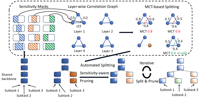
Figure 3: Iterative splitting and pruning. Starting from a shared backbone, we compute the layer-wise sensitivity mask $\mathcal{M}$ for each subtask loss, and calculate pair-wise IoU score $J$ across different subtasks for the layer-wise correlation graph. Model is split at the layer with a small minimal cutting threshold (MCT), and, then, is pruned globally. Applying splitting and pruning in an iterative fashion leads to the final Split-Ensemble architecture that satisfies the cost constraints.

4.1 Correlation-based automated splitting

Intuitively, with the subtasks split from the original task, submodels should be able to share the low-level features learned in the early layers of the model, while using diverse high-level filters in later layers in each subtask. Given the difficulty of merging independently training submodels during training, we instead start our ensemble training from a single backbone model for the original task. We consider all the submodels using the same architecture with the same parameters of the backbone model, only with independent fully-connected (FC) classifiers at the end.

The question therefore becomes: On which layer shall we split a submodel from the shared backbone? Here we propose an automated splitting strategy that can learn a proper splitting architecture given the split subtasks. Intuitively, two submodels can share the same layer if they are both benefiting from the existing weights (i.e., removing a filter will hurt both models simultaneously). Otherwise, if the weight sensitive to submodel 1 can be removed for submodel 2 without harm, and vice versa, then it would be worth splitting the architecture and shrinking the submodels separately. We therefore formulate our splitting strategy based on the overlapping of sensitive weight elements for each subtask. Specifically, for submodels share the same layer with weight $W$. We perform a single-shot sensitivity estimation of all the weight elements in $W$ on the subtask loss $\mathcal{L}_{CB}^{i}$ of each submodel $i$ respectively. The sensitivity $s_{j}^{i}$ of element $w_{j}$ on submodel $i$ is measured as

$$s_{j}^{i}=\frac{|g(w_{j})|}{\sum_{w_{k}\in W}|g(w_{k})|},\ g(w_{j})=w_{j}\nabla_{w_{j}}\mathcal{L}_{CB}^{i}(W),$$ (5)

following the criteria proposed in SNIP (Lee et al., 2019). Then we perform a Top-K masking to select the $K$ weight elements with the largest sensitivity, forming a sensitive mask $\mathcal{M}_{i}$ for submodel $i$. Then weight element lies in the intersection of the two masks $\mathcal{M}_{i}\cap\mathcal{M}_{j}$ are sensitive for both subtasks, while other elements in the union $\mathcal{M}_{i}\cup\mathcal{M}_{j}$ but not in the intersection are only sensitive to one subtask. We use the Intersection over Union (IoU) score to measure the pair-wise mask correlation as $J_{ij}=\frac{|\mathcal{M}_{i}\cap\mathcal{M}_{j}|}{|\mathcal{M}_{i}\cup\mathcal{M}_{j}|}$, where $|\cdot|$ denotes the cardinality of a set. It has been observed in previous multi-task pruning work that pruning mask correlations will be high in the early layers and drop sharply towards later layers (Sun et al., 2022), as later layers learn more high-level features that are diverse across subtasks. A pair of submodels can be split at the earliest layer that the IoU score drops below a predefined threshold. The architecture and parameters of the new branch are initialized as the exact copy of the original layers it is splitting from, which guarantees the same model functionality before and after the split. The branches will then be updated, pruned, and further split independently after the splitting is performed given their low correlation.

In the case of multiple submodels, we compute the pairwise IoU score between each pair of submodels, and build a “correlation graph” for each layer. The correlation graph is constructed as a weighted complete graph $C=(V,E)$ with each submodel being a node $v\in V$, and the IoU score between two submodels $J_{uv}$ is assigned as the weight of the edge $(u,v)\in E$ between the corresponding nodes. Then a split of the model is equivalent to performing a cut on the correlation graph to form two separated subgraphs $S$ and $T$. Here we propose a measurement of “Minimal Cutting Threshold” (MCT), which is the minimal correlation threshold for edge removal that can cut the correlation graph into two. Formally, the MCT of a correlation graph $C$ is defined as

$$MCT(C)=\min_{S,T}\left[\max_{u\in S,v\in T,(u,v)\in E}J_{uv}\right],\ s.t.\ S+T=V.$$ (6)

A small MCT indicates that a group of submodels has a weak correlation with the rest, therefore they can be separated from the shared architecture. In practice, we will iteratively split the earliest layer with an MCT lower than a predefined value in a branch shared by multiple submodels, until all submodels have individual branches at the end. The splitting strategy will turn a single backbone model into a tree-like architecture, as illustrated in Figure 3.

4.2 Sensitivity-aware global pruning

To remove the redundancy in the submodels for simpler subtasks, we perform global structural pruning on the Split-Ensemble architecture. We perform structural sensitivity estimation on a group of weight element $w_{s}$ belonging to a structure $\mathcal{S}$ for the loss $\mathcal{L}_{CB}^{i}$ of each subtask $i$. We utilize the Hessian importance estimation (Yang et al., 2023), which is computed as

$$\mathcal{I}^{i}(\mathcal{S})=\left(\sum_{s\in\mathcal{S}}w_{s}\nabla_{w_{s}}\mathcal{L}_{CB}^{i}(w_{s})\right)^{2}.$$ (7)

It has been shown that this importance score is comparable across different layers and different types of structural components (Yang et al., 2023), making it a good candidate for global pruning. Then, we greedily prune a fixed number of filters with the smallest $\mathcal{I}^{i}$ in submodel $i$. In the case where multiple submodels are sharing the structure, we separately rank the importance of this structure in each submodel, and will only prune the filters that are prunable for all the submodels sharing it.

Putting everything together, we iteratively perform the aforementioned automated splitting and pruning process during the training of the Split-Ensemble model. Splitting and pruning are performed alternatively. Removing commonly unimportant structures will reduce the sensitivity correlation in the remaining parameters, enabling further splitting of the submodels. In contrast, having a new split enables additional model capacity for further pruning. The splitting will be fixed when all submodels have an individual branch towards later layers of the model. Pruning will be stopped when the Floating-point Operations (FLOPs) of the Split-Ensemble architecture meet a predefined computational budget, typically the FLOPs of the original backbone model. The Split-Ensemble model will then train with the fixed model architecture for the remaining training epochs. The detailed process of Split-Ensemble training is provided in the pseudo-code in Algorithm 1 of Appendix B.

5 Experiments

Here we compare the accuracy of Split-Ensemble with baseline single model and ensemble methods in Section 5.1, and showcase the OOD detection performance on various datasets in Section 5.2. We provide ablation studies on the design choices of using OOD-aware target in subtask training and selecting MCT threshold for iterative splitting in Section 5.3. Detailed experiment settings are available in Appendix A.

5.1 Performance on classification accuracy

We train Split-Ensemble on CIFAR-10, CIFAR-100, and Tiny-ImageNet dataset and evaluate its classification accuracy. The results are compared with baseline single model, deep ensemble with 4x submodels, and other parameter-efficient ensemble methods (if results available) in Table 1. On CIFAR-100, we notice that Deep Ensemble with independent submodels achieves the best accuracy. Other efficient ensembles cannot reach the same level of accuracy with shared parameters, yet still require the same amount of computation. Our Split-Ensemble, on the other hand, beats not only single model but also other efficient ensemble methods, without additional computation cost. Additional results on CIFAR-10 and Tiny-ImageNet show that Split-Ensemble can bring consistent performance gain over single model, especially for difficult tasks like Tiny-ImageNet, where a single model cannot learn well. The improved performance comes from our novel task-splitting training objective, where each submodel can learn faster and better on simpler subtasks, leading to better convergence. The iterative splitting and pruning process further provides efficient architecture for the Split-Ensemble to achieve high performance without the computational overhead.

Table 1: Classification performance on CIFAR-100, CIFAR-10, and Tiny-ImageNet datasets. Best score for each metric in bold, second-best underlined. We implement all baselines using default hyperparameters. All accuracies are given in percentage with ResNet-18/ResNet-34 as backbone

Method	FLOPs	CIFAR-10 Acc ($\uparrow$)	CIFAR-100 Acc ($\uparrow$)	Tiny-IMNET Acc ($\uparrow$)
Single Network	1x	94.7 / 95.2	75.9 / 77.3	26.1 / 25.7
Deep Ensemble	4x	95.7 / 95.5	80.1 / 80.4	44.6 / 43.9
MC-Dropout	4x	93.3 / 90.1	73.3 / 66.3	58.1 / 60.3
MIMO	4x	86.8 / 87.5	54.9 / 54.6	46.4 / 47.8
MaskEnsemble	4x	94.3 / 90.8	76.0 / 64.8	61.2 / 62.6
BatchEnsemble	4x	94.0 / 91.0	75.5 / 66.1	61.7 / 62.3
FilmEnsemble	4x	87.8 / 94.3	77.4 / 77.2	51.5 / 53.2
Split-Ensemble (Ours)	1x	95.5 / 95.6	77.7 / 77.4	51.6 / 47.6

5.2 Performance on OOD detection

As we focus the design of Split-Ensemble on better OOD-aware training, here we compare the OOD detection performance of the Split-Ensemble model with a single model and naive ensemble baselines with ResNet-18 backbone. All models are trained using the same code under the same settings. For OOD detection score computation, we use the max softmax probability for the single model, max softmax probability of the mean logits for the naive ensemble, and use the probability score proposed in Section 3.3 for our Split-Ensemble. A single threshold is used to detect OOD with score lower than the threshold. Table 2 shows the comparison between the OOD detection performance. We can clearly see that our method can outperform single model baseline and 4$\times$ larger Naive ensemble across all of the benchmarks. This improvement shows our OOD-aware training performed on each subtask can generalize to unseen OOD data, without using additional data at the training time.

Table 2: OOD detection results. Models trained on ID dataset are evaluated against multiple OOD datasets. The results are reported for models with ResNet-18 backbone. FPR and detection error are evaluated with the threshold achieving 95% TPR.

ID	OOD	FPR	Det. Error	AUROC	AUPR
dataset	dataset	(95% TPR)$\downarrow$	(95% TPR) $\downarrow$	$\uparrow$	$\uparrow$
CIFAR-10		Single Model / Naive Ensemble (4x) / Split-Ensemble (ours)
	CIFAR-100	56.9 / 50.6 / 47.9	30.9 / 27.8 / 26.4	87.4 / 87.8 / 89.6	85.7 / 85.6 / 89.5
	TinyImageNet (crop)	30.9 / 29.9 / 39.2	17.9 / 17.4 / 22.1	93.1 / 94.4 / 94.9	96.0 / 93.8 / 96.4
	TinyImageNet (resize)	54.9 / 50.3 / 46.0	29.9 / 27.7 / 25.5	87.5 / 89.3 / 91.7	86.2 / 88.0 / 92.8
	SVHN	48.4 / 31.1 / 30.5	17.0 / 12.2 / 12.1	91.9 / 93.8 / 95.2	84.0 / 85.8 / 91.9
	LSUN (crop)	27.5 / 18.7 / 37.5	16.3 / 11.9 / 21.3	92.1 / 95.9 / 95.3	96.8 / 94.8 / 96.8
	LSUN (resize)	49.4 / 34.6 / 33.2	27.2 / 19.8 / 19.1	90.5 / 93.4 / 94.5	90.7 / 93.3 / 95.7
	Uniform	83.0 / 85.3 / 63.7	76.3 / 78.1 / 58.7	91.9 / 88.5 / 92.5	99.2 / 98.8 / 99.3
	Gaussian	9.4 / 95.4 / 33.0	9.3 / 87.2 / 30.5	97.7 / 85.6 / 95.7	99.8 / 98.3 / 99.6
	Mean	45.1 / 49.5 / 41.4	28.1 / 35.3 / 27.0	91.5 / 91.1 / 93.7	92.3 / 92.3 / 95.3
CIFAR-100	CIFAR-10	76.2 / 78.6 / 78.5	40.6 / 41.8 / 41.7	80.5 / 80.3 / 79.2	83.2 / 82.2 / 81.7
	TinyImageNet (crop)	66.1 / 77.5 / 58.1	41.2 / 49.7 / 31.6	85.8 / 80.3 / 88.4	88.3 / 82.2 / 90.0
	TinyImageNet (resize)	68.2 / 78.6 / 72.1	38.9 / 41.8 / 38.6	84.4 / 77.5 / 82.7	86.9/ 79.3 / 84.6
	SVHN	60.6 / 75.2 / 75.0	20.4 / 24.5 / 24.4	87.7 / 83.3 / 81.2	81.1 / 74.4 / 69.9
	LSUN (crop)	70.9 / 84.7 / 64.7	44.8 / 49.3 / 34.9	76.7 / 76.7 / 85.3	86.6 / 79.9 / 86.6
	LSUN (resize)	66.7 / 79.1 / 72.0	35.9 / 42.1 / 38.5	85.4 / 78.3 / 83.2	87.9 / 80.1 / 85.6
	Uniform	100.0 / 100.0 / 95.0	90.9 / 90.9 / 65.9	59.2 / 69.1 / 88.3	95.2 / 91.6 / 98.8
	Gaussian	100.0 / 100.0 / 99.6	90.9 / 72.5 / 90.9	40.6 / 59.2 / 63.1	92.0 / 95.2 /95.5
	Mean	76.1 / 84.2 / 74.0	48.9 / 52.3 / 45.7	73.9 / 75.6 / 82.0	87.3 / 83.7 / 86.6
Tiny-IMNET	CIFAR-10	99.3 / 97.7 / 100.0	33.3 / 50.3 / 33.3	56.5 / 46.7 / 81.2	48.9 / 48.6 / 82.7
	CIFAR-100	99.2 / 97.5 / 100.0	33.3 / 50.3 / 9.1	54.6 / 46.1 / 72.6	45.5 / 47.5 / 51.9
	SVHN	95.2 / 97.5 / 100.0	16.1 / 20.1 / 16.1	64.8 / 46.5 / 83.6	38.1 / 26.6 / 80.2
	LSUN (crop)	100.0 / 97.5 / 94.0	33.3 / 50.3 / 33.3	28.9 / 45.9 / 80.2	25.9 / 48.8 / 78.5
	LSUN (resize)	99.8 / 97.8 / 100.0	50.3 / 50.3 / 33.3	44.9 / 45.9 / 76.3	36.5 / 47.4 / 77.2
	Uniform	100.0 / 90.2 / 100.0	83.3 / 73.5 / 83.3	24.2 / 43.9 / 63.8	77.7 / 90.2 / 92.5
	Gaussian	100.0 / 96.7 / 100.0	83.3 / 73.5 / 83.3	25.4 / 43.8 / 49.3	78.1 / 89.9 / 88.1
	Mean	99.1 / 96.4 / 99.1	45.1 / 52.6 / 46.4	42.8 / 45.8 / 72.4	50.1 / 57.0 / 78.7

5.3 Ablation studies

In this section, we provide the results of exploring the use of OOD-aware target (Equation (3)) and the impact of MCT threshold in automated splitting (Section 4.1). Due to space limitation, we put additional results on ablating the influence of the number of subtask splittings and the grouping of classes for each subtask in Appendix C.

Table 3: Ablation on OOD-aware subtask training. Models are trained on CIFAR-100. OOD detection is against the CIFAR-10 dataset.

# splits	OOD class target	Accuracy	AUROC
2	One-hot	71.0	76.0
	OOD-aware	77.7	78.1
4	One-hot	77.2	77.5
	OOD-aware	78.0	78.2
5	One-hot	77.7	77.3
	OOD-aware	77.9	78.1

OOD-aware target

In Section 3.2, we propose to use an outlier exposure-inspired target for the inputs belonging to the OOD class, so as to better calibrate the confidence during submodel training. Table 3 compares the results of training Split-Ensemble submodels with the original one-hot labels for OOD class vs. the proposed OOD-aware targets. No matter how many subtask splittings we use, using the OOD-aware target significantly improved the AUROC for OOD detection, while also helping the ID accuracy of the model. The results indicate that having an explicit OOD class is inadequate for the submodel to learn generalizable OOD detection, and the OOD-aware training objective is effective. Improving submodel OOD detection also helps ensemble accuracy as the submodels can better distinguish their ID classes from others.

Table 4: Ablation on MCT thresholds. Models are trained on CIFAR-100 with 5 subtask splits. OOD detection is against CIFAR-10. Detailed split architectures are visualized in Appendix C.

MCT threshold	0.0 (all-share)	0.1	0.2	0.4	0.7
Accuracy	76.2	77.9	78.4	77.9	77.9
AUROC	76.7	78.0	78.8	79.9	78.9

Automated Splitting Threshold

In Section 4.1, we design our automatic splitting strategy as splitting a (group of) submodels from the backbone when the MCT at a certain layer drops below a predefined threshold. The choice of this MCT threshold is therefore impactful on the final architecture and performance of the Split-Ensemble model. Table 4 explores the model performance as we increase the MCT threshold from 0.0 (all-share). As the threshold increases, the models can branch out easier in earlier layers (see architectures in Appendix C), which improves the flexibility for the submodels to learn diverse features for the OOD-aware subtasks, leading to improvements in both ID accuracy and OOD detection. However, more and earlier branches require the use of aggressive pruning to maintain the ensemble under cost constraints, which eventually hurts the model performance. A threshold around 0.4 gives a good balance with adequate diversity (as deep ensemble) and high efficiency (as single model) to the final Split-Ensemble model, leading to good performance.

6 Conclusions

In this paper, we introduced the Split-Ensemble method, a new approach to improve single-model accuracy and OOD detection without additional training data or computational overhead. By dividing the learning task into complementary subtasks, we enabled OOD-aware learning without external data. Our split-and-prune algorithm efficiently crafted a tree-like model architecture for the subtasks, balancing performance and computational demands. Empirical results validated the effectiveness of the Split-Ensemble. We hope this work opens up a promising direction for enhancing real-world deep learning applications with task and model splitting, where subtasks and submodel architectures can be co-designed to learn better calibrated efficient models on complicated tasks.

Acknowledgement

We would like to acknowledge the support from Berkeley Deep Drive and Panasonic for this work.

Appendix A Experimental Setup

A.1 Datasets and metrics.

We perform classification tasks on four popular image classification benchmarks, including CIFAR-10, CIFAR-100 (Krizhevsky, 2009), Tiny ImageNet (Deng et al., 2009) and ImageNet (Krizhevsky et al., 2012) datasets. Additionally, we examine our method on the challenging long-tailed dataset, CIFAR10-LT and CIFAR100-LT datasets (Cao et al., 2019).

• CIFAR10 is a collection of 60,000 32x32 color images spanning 10 different classes, such as automobiles, birds, and ships, with each class containing 6,000 images. It is commonly used in machine learning and computer vision tasks for object recognition, serving as a benchmark to evaluate the performance of various algorithms.

• CIFAR100 is a diverse and challenging image dataset consisting of 60,000 32x32 color images spread across 100 different classes. Each class represents a distinct object or scene, making it a comprehensive resource for fine-grained image classification and multi-class tasks. CIFAR-100 is widely used in machine learning research to evaluate the performance of models in handling a wide range of object recognition challenges.

• Tiny ImageNet is a compact but diverse dataset containing thousands of small-sized images, each belonging to one of 200 categories. This dataset serves as a valuable resource for tasks like image classification, with each image encapsulating a rich variety of objects, animals, and scenes, making it ideal for training and evaluating machine learning models.

• CIFAR10-LT & CIFAR100-LT are the long-tailed version of CIFAR10 and CIFAR100 datasets with imbalance ratio $\rho=100$.

For the out-of-distribution detection task, we use CIFAR-10, and CIFAR-100, Tiny ImageNet as in-distribution datasets, and use CIFAR-10, CIFAR-100, Tiny ImageNet, SVHN, LSUN, Gaussian Noise, Uniform Noise, as out-of-distribution datasets. Additionally, we adopt a more challenging OOD detection benchmark, named semantically coherent out-of-distribution detection (SC-OOD) (Yang et al., 2021).

• SVHN. The Street View House Numbers (SVHN) dataset is a comprehensive collection of house numbers captured from Google Street View images. It consists of over 600,000 images of house numbers from real-world scenes, making it a critical resource for tasks like digit recognition and localization. SVHN’s diversity in backgrounds, fonts, and lighting conditions makes it a challenging but vital dataset for training and evaluating machine learning algorithms in the domain of computer vision.

• LSUN. The LSUN (Large-scale Scene Understanding) dataset is a vast collection of high-resolution images, primarily focused on scenes and environments. It encompasses a diverse range of scenes, including bedrooms, kitchens, living rooms, and more. LSUN serves as a valuable resource for tasks such as scene recognition and understanding due to its extensive coverage of real-world contexts and rich visual content.

• Gaussian Noise and Uniform Noise. After introducing Gaussian Noise or Uniform Noise to the dataset, we obtain a modified dataset, which is then utilized as an OOD dataset for our experiments. We implement this operation using the library from Kirchheim et al. (2022).

• SC-OOD benchmark. The SC-OOD (Semantically Coherent Out-of-Distribution) benchmark is designed for evaluating out-of-distribution detection models by focusing on semantic coherence. This benchmark addresses the limitations of traditional benchmarks that often require models to distinguish between objects with similar semantics from different datasets, such as CIFAR dogs and ImageNet dogs.

We use five key metrics to evaluate the performance of ID classification and OOD detection tasks.

• Accuracy. This is defined as the ratio of the number of correct predictions to the total number of predictions made. We report top-1 classification accuracy on the test(val) sets of ID datasets.

• FPR (95% TPR). This metric stands for ’False Positive Rate at 95% True Positive Rate’. It measures the proportion of negative instances that are incorrectly classified as positive when the true positive rate is 95%. A lower FPR at 95% TPR is desirable as it indicates fewer false alarms while maintaining a high rate of correctly identified true positives.

• Detection Error (95% TPR). Detection Error at 95% TPR is a metric that quantifies the overall error rate when the model achieves a true positive rate of 95%. It combines false negatives and false positives to provide a single measure of error. Lower detection error values indicate better performance, as the model successfully identifies more true positives with fewer errors.

• AUROC is short for Area Under the Receiver Operating Characteristic Curve(AUROC). This metric measures the ability of a model to distinguish between in-distribution and OOD samples. The ROC curve plots the true positive rate against the false positive rate at various threshold settings. The AUROC is the area under this curve, with higher values (closer to 1.0) indicating better discrimination between in-distribution and OOD samples.

• AURP is short for Area Under the Precision-Recall Curve (AUPR), this metric is particularly useful in scenarios where there is a class imbalance (a significant difference in the number of in-distribution and OOD samples). It plots precision (the proportion of true positives among positive predictions) against recall (the proportion of true positives identified). Higher AUPR values suggest better model performance, especially in terms of handling the balance between precision and recall.

Implementation Details.

Our Split Ensemble model was trained over 200 epochs using a single NVIDIA A100 GPU with 80GB of memory, for experiments involving CIFAR-10, CIFAR-100, and Tiny ImageNet datasets. For the larger-scale ImageNet dataset, we employ 8 NVIDIA A100 GPUs, each with 80GB memory, to handle the increased computational demands. We use an SGD optimizer with a momentum of 0.9 and weight decay of 0.0005. We also adopt a 200-epoch cosine learning rate schedule with 10 warm-up epochs and a batchsize of 256. Our experiments typically run for approximately 2 hours on both CIFAR-10 and CIFAR-100 datasets, whereas on the Tiny ImageNet and ImageNet datasets, they take approximately 10 hours and 24 hours, respectively. We employ data augmentation techniques such as rotation and flip during the training phase, while the testing phase does not involve data augmentation. As for the backbone models in our experiments, we utilize the standard ResNet-18 and ResNet-34 architectures. We heuristically decide the number of submodels in the Split-Ensemble via ablation study, where we find 8 submodels for ImageNet-1K and 5 submodels for other datasets leads to the best performance in both ID and OOD detection. The classes are grouped based on semantic similarity into subtasks for the submodels to learn.

Appendix B Pseudo code for Split-Ensemble training

The Pseudo code of Split-Ensemble training is available in Algorithm 1.

Algorithm 1 Training the Split-Ensemble model

1:# Initialization and preparation

2:Load dataset $\{X,Y\}$

3:Subtask label conversion $Y\rightarrow\hat{Y}_{i}$ as Equation (3)

4:Initialize Split-Ensemble $F$ with all submodels $f_{i}$ sharing backbone model

5:# Split ensemble training

6:while Training do

7:     Update $F$ to minimize $\mathcal{L}_{ens}$ in Equation (4) with SGD

8:     # Iterative splitting and pruning

9:     if Epoch % Prune_Interval == 0 then

10:         # Splitting

11:         if $\exists$ branch in $F$ with multiple submodel $f_{i}$ sharing all layers then

12:              for Layers in the branch shared only by $f_{i}$ do

13:                  Compute sensitivity map following Equation (5) for each $f_{i}$

14:                  Compute MCT of the layer following Equation (6)

15:                  if MCT $<$ threshold then

16:                       Split branch at the layer

17:                       Break                                          

18:         # Pruning

19:         if FLOPs $>$ target then

20:              for All submodels $f_{i}$ do

21:                  Compute $\mathcal{I}^{i}_{\mathcal{S}}$ for all $\mathcal{S}$ following Equation (7)

22:                  Rank $\mathcal{I}^{i}_{\mathcal{S}}$ to decide prunable structures with $\min_{\mathcal{S}}\mathcal{I}^{L}_{\mathcal{S}}$

23:                  Remove structures prunable for (all) corresponding submodels                             

Appendix C Additional results and visualizations

In this section, we provide additional results in comparison with baseline methods in different settings as well as ablation results on our design choices following the discussion in Section 5.3.

Subtask grouping strategy

In Section 3.1, we propose to use the group of classes that are semantically-close to form each subtasks of the complementary task splitting. Here we verify this intuition against have random assignment of classes to each subtask. As illustrated in Table 5, having semantically-close subtask grouping significantly improves the OOD detection ability of the Split-Ensemble model over that of random grouping. This improvement is more significant with more subtask splittings. We believe that semantic grouping of subtasks help the submodels to better learn the difference between ID classes and OOD classes of the subtask, as the semantically-close ID classes may share more distinct features comparing to other classes.

Table 5: Ablation on subtask grouping strategy. Models are trained on CIFAR-100. OOD detection is against the CIFAR-10 dataset.

# splits	Subtask grouping	Accuracy	AUROC
2	Random	77.3	78.9
	Semantic	77.8	79.6
4	Random	77.3	77.5
	Semantic	77.5	79.1
5	Random	77.4	77.3
	Semantic	77.9	78.9

Number of subtask splittings

We conducted an analysis to explore the impact of the number of splits on the accuracy and OOD detection performance of the Split-Ensemble model. Unlike traditional ensemble that repeatedly learn the same task with more submodels, Split-Ensemble always learns a complementary subtask splitting corresponding to the original task. Increasing the amount of splits will therefore enable each submodel to learn a simpler subtasks with less ID classes, intuitively leading to a model architecture with more yet smaller branches. As shown in Table 6, the Split-Ensemble accuracy is not sensitive to the number of splits, showing the scalability of our learning algorithm. For OOD detection, a larger number of splits enables each submodel to learn its OOD-aware objective more easily, therefore leading to better AUROC. Yet the performance may suffer from aggressive pruning with too much branches in the Split-Ensemble, as observed with a large MCT threshold in Table 4. An interesting future direction would be automatically design the amount of subtask splitting and the grouping of each subtask during the training process to better fit the subtasks to the Split-Ensemble architecture.

Table 6: Ablation on number of splits. Models are trained on CIFAR-100. OOD detection is against the CIFAR-10 dataset. All models are constrained with single-model computation cost.

# splits	2	4	5	8	10
Accuracy	77.7	78.0	77.9	77.5	77.3
AUROC	78.1	78.2	79.9	80.4	77.3

Additional classification results on ImageNet

We perform classification on the large-scale ImageNet1K dataset to examine our method. As shown in Table. 7, our method continues to outperform the single and $4\times$ more costly ensemble methods, demonstrating the effectiveness of our design.

Table 7: Classification performance on ImageNet1K dataset. The results are reported for models with ResNet-18 backbone. Best score in bold.

Method	Acc
Single	69.0
Naive Ensemble	69.4
Split-Ensemble (ours)	70.9

Additional classification and OOD detection results on CIFAR10-LT with SC-OOD benchmark

We assess our method on CIFAR10-LT, a complex long-tailed dataset, to evaluate its robustness. As evidenced in Table 8, our approach consistently outperforms in all four metrics. Remarkably, this is achieved with only a quarter of the computational cost compared to baseline methods. This underscores our model’s efficiency and effectiveness in managing intricate classification and OOD detection tasks.

Table 8: Comparison between previous state-of-the-art ensemble-based methods and ours on the SC-OOD CIFAR10-LT benchmarks. The results are reported for models with ResNet-18 backbone. Best score in bold, second best underlined.

Method	Accuracy $\uparrow$	FPR95 $\downarrow$	AUROC $\uparrow$	AUPR $\uparrow$
Naive Ensemble	12.7	98.4	45.3	50.9
MC-Dropout	63.4	90.6	66.6	66.1
MIMO	35.7	96.3	55.1	56.9
MaskEnsemble	67.7	89.0	66.82	67.4
BatchEnsemble	70.1	87.45	68.0	68.7
FilmEnsemble	72.5	84.32	75.5	76.0
Split-Ensemble (ours)	73.7	80.5	81.7	77.6

Table 9: Comparison between previous state-of-the-art single-model-based methods and ours on the SC-OOD CIFAR10 benchmarks. The results are reported for models with ResNet-18 backbone. Best score in bold, second best underlined.

Method	Additional Data	FPR95 $\downarrow$	AUROC $\uparrow$	AUPR $\uparrow$
ODIN		52.0	82.0	85.1
EBO		50.0	83.8	85.1
OE		50.5	88.9	87.8
MCD		73.0	83.9	80.5
UDG		55.6	90.7	88.3
UDG		36.2	93.8	92.6
Split-Ensemble (ours)		45.5	91.1	89.9

Additional OOD detection results on CIFAR10 with SC-OOD benchmark

We further compare our methods with previous state-of-the-art methods. In Table. 9, our Split-Ensemble model outperforms single-model approaches in OOD detection without incurring additional computational costs or requiring extra training data. Its consistent high performance across key metrics highlights its robustness and efficiency, underscoring its practical utility in OOD tasks. In Table. 10, our Split-Ensemble model consistently outshines other ensemble-based methods in both image classification and OOD detection, achieving top rankings across all key metrics, which underscores the model’s efficiency and effectiveness.

Table 10: Comparison between previous state-of-the-art ensemble-based methods and ours on the SC-OOD CIFAR10 benchmarks. The results are reported for models with ResNet-18 backbone. Best score in bold, second best underlined.

Method	Additional Data	FPR95 $\downarrow$	AUROC $\uparrow$	AUPR $\uparrow$
Naive Ensemble	4x	42.3	90.4	90.6
MC-Dropout	4x	54.9	88.7	88.0
MIMO	4x	73.7	83.5	80.9
MaskEnsemble	4x	53.2	87.7	87.9
BatchEnsemble	4x	50.4	89.2	88.6
FilmEnsemble	4x	42.6	91.5	91.3
Split-Ensemble (ours)	1x	45.5	91.1	89.9

Model activation map visualization

We visualize the learned feature map activations of a Split-Ensemble model across different layers using Score-CAM (Wang et al., 2020) in Figure 4. The shared feature maps, delineated by dashed lines, represent the common features extracted across different submodels, emphasizing the model’s capacity to identify and leverage shared representations. The distinct feature maps outside the dashed boundaries correspond to specialized features pertinent to individual sub-tasks, demonstrating the Split-Ensemble model’s ability to focus on unique aspects of the data when necessary. This visualization underscores the effectiveness of the Split-Ensemble architecture, highlighting its dual strength in capturing both shared and task-specific features within a single, cohesive framework, thereby bolstering its robustness and adaptability in handling diverse image classification and OOD detection tasks.

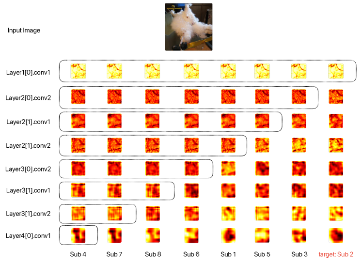
Figure 4: Visualization of Split-Ensemble’s learned features using Score-CAM. The number of splits is set to 8 and the model is trained on ImageNet1K with ResNet-18 as backbone. The feature maps within the dashed lines across the layers indicate shared representations. The input image’s class is ’Angora’, targeted by submodel 2.

Model architecture visualization

We visualize the Split-Ensemble models achieved under different MCT thresholds in Figure 5, as discussed in Table 4 of Section 5.3. Models here use 5 splits and are trained on CIFAR-100 dataset with ResNet-18 as backbone. With a larger MCT threshold, the model will split into more branches at earlier layers. Meanwhile the model will also be pruned more aggressively to keep the overall computation cost unchanged. We can clearly see that with a proper MCT threshold, our method can learn a tree-like Split-Ensemble architecture with different submodels branching out at different layers, as designed by our iterative splitting and pruning algorithm in Section 4.

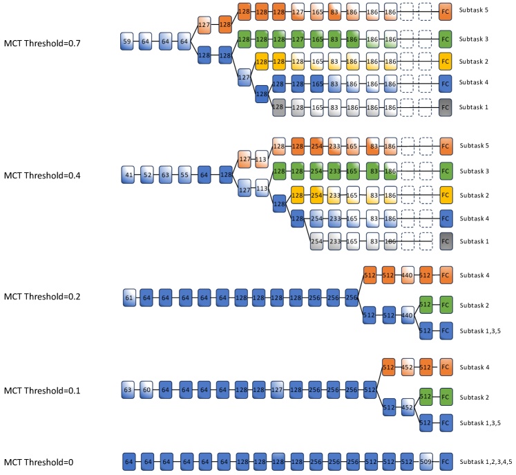
Figure 5: Visualization of Split-Ensemble architectures under different MCT threshold. The number of splits is set to 5. Number in each block denotes the number of filters in the layer.

References

- Cao et al. (2019) Kaidi Cao, Colin Wei, Adrien Gaidon, Nikos Arechiga, and Tengyu Ma. Learning imbalanced datasets with label-distribution-aware margin loss. In Advances in Neural Information Processing Systems, 2019.
- Cui et al. (2019) Yin Cui, Menglin Jia, Tsung-Yi Lin, Yang Song, and Serge Belongie. Class-balanced loss based on effective number of samples. In Proceedings of the IEEE/CVF Conference on Computer Vision and Pattern Recognition (CVPR), pp. 9268–9277, 2019.
- Deng et al. (2009) Jia Deng, Wei Dong, Richard Socher, Li-Jia Li, Kai Li, and Li Fei-Fei. Imagenet: A large-scale hierarchical image database. In Proceedings of the IEEE/CVF Conference on Computer Vision and Pattern Recognition (CVPR), pp. 248–255, 2009.
- Ding et al. (2021) Ke Ding, Xin Dong, Yong He, Lei Cheng, Chilin Fu, Zhaoxin Huan, Hai Li, Tan Yan, Liang Zhang, Xiaolu Zhang, and Linjian Mo. Mssm: A multiple-level sparse sharing model for efficient multi-task learning. In Proceedings of the International ACM SIGIR Conference on Research and Development in Information Retrieval, pp. 2237–2241, 2021.
- Durasov et al. (2021) Nikita Durasov, Timur Bagautdinov, Pierre Baque, and Pascal Fua. Masksembles for uncertainty estimation. In Proceedings of the IEEE/CVF Conference on Computer Vision and Pattern Recognition (CVPR), pp. 13539–13548, 2021.
- Gal & Ghahramani (2016) Yarin Gal and Zoubin Ghahramani. Dropout as a bayesian approximation: Representing model uncertainty in deep learning. In International Conference on Machine Learning, 2016.
- Havasi et al. (2021) Marton Havasi, Rodolphe Jenatton, Stanislav Fort, Jeremiah Zhe Liu, Jasper Snoek, Balaji Lakshminarayanan, Andrew M Dai, and Dustin Tran. Training independent subnetworks for robust prediction. In International Conference on Learning Representations (ICLR), 2021.
- Hendrycks & Dietterich (2019) Dan Hendrycks and Thomas Dietterich. Benchmarking neural network robustness to common corruptions and perturbations. arXiv:1903.12261, 2019.
- Hendrycks et al. (2018) Dan Hendrycks, Mantas Mazeika, and Thomas Dietterich. Deep anomaly detection with outlier exposure. arXiv:1812.04606, 2018.
- Hendrycks et al. (2022) Dan Hendrycks, Steven Basart, Mantas Mazeika, Andy Zou, Joseph Kwon, Mohammadreza Mostajabi, Jacob Steinhardt, and Dawn Song. Scaling out-of-distribution detection for real-world settings. In Proceedings of the International Conference on Machine Learning, pp. 8759–8773, 2022.
- Jeong & Kim (2020) Taewon Jeong and Heeyoung Kim. OOD-MAML: Meta-learning for few-shot out-of-distribution detection and classification. In Advances in Neural Information Processing Systems, volume 33, pp. 3907–3916, 2020.
- Kirchheim et al. (2022) Konstantin Kirchheim, Marco Filax, and Frank Ortmeier. Pytorch-ood: A library for out-of-distribution detection based on pytorch. In Proceedings of the IEEE/CVF Conference on Computer Vision and Pattern Recognition (CVPR) Workshops, pp. 4351–4360, June 2022.
- Krizhevsky (2009) Alex Krizhevsky. Learning multiple layers of features from tiny images. Technical report, University of Toronto, 2009.
- Krizhevsky & Hinton (2009) Alex Krizhevsky and Geoffrey Hinton. Learning multiple layers of features from tiny images. Technical report, Citeseer, 2009.
- Krizhevsky et al. (2012) Alex Krizhevsky, Ilya Sutskever, and Geoffrey E Hinton. Imagenet classification with deep convolutional neural networks. In Advances in neural information processing systems, pp. 1097–1105, 2012.
- Lakshminarayanan et al. (2017) Balaji Lakshminarayanan, Alexander Pritzel, and Charles Blundell. Simple and scalable predictive uncertainty estimation using deep ensembles. arXiv:1612.01474, 2017.
- Lane et al. (2007) Ian Lane, Tatsuya Kawahara, Tomoko Matsui, and Satoshi Nakamura. Out-of-domain utterance detection using classification confidences of multiple topics. IEEE Transactions on Audio, Speech, and Language Processing, 15(1):150–161, 2007.
- Lee et al. (2019) Namhoon Lee, Thalaiyasingam Ajanthan, and Philip HS Torr. SNIP: Single-shot network pruning based on connection sensitivity. International Conference on Learning Representations (ICLR), 2019.
- Liang et al. (2017) Shiyu Liang, Yixuan Li, and Rayadurgam Srikant. Enhancing the reliability of out-of-distribution image detection in neural networks. arXiv:1706.02690, 2017.
- Papadopoulos et al. (2021) Aristotelis-Angelos Papadopoulos, Mohammad Reza Rajati, Nazim Shaikh, and Jiamian Wang. Outlier exposure with confidence control for out-of-distribution detection. Neurocomputing, 441:138–150, June 2021.
- Sehwag et al. (2021) Vikash Sehwag, Mung Chiang, and Prateek Mittal. SSD: A unified framework for self-supervised outlier detection. In International Conference on Learning Representations (ICLR), 2021.
- Sharma et al. (2017) Sahil Sharma, Ashutosh Jha, Parikshit Hegde, and Balaraman Ravindran. Learning to multi-task by active sampling. arXiv:1702.06053, 2017.
- Sun et al. (2021) Guolei Sun, Thomas Probst, Danda Pani Paudel, Nikola Popović, Menelaos Kanakis, Jagruti Patel, Dengxin Dai, and Luc Van Gool. Task switching network for multi-task learning. In Proceedings of the IEEE/CVF International Conference on Computer Vision (ICCV), pp. 8291–8300, October 2021.
- Sun et al. (2022) Xinglong Sun, Ali Hassani, Zhangyang Wang, Gao Huang, and Humphrey Shi. DiSparse: Disentangled sparsification for multitask model compression. In Proceedings of the IEEE/CVF Conference on Computer Vision and Pattern Recognition (CVPR), pp. 12382–12392, 2022.
- Turkoglu et al. (2022) Mehmet Ozgur Turkoglu, Alexander Becker, Hüseyin Anil Gündüz, Mina Rezaei, Bernd Bischl, Rodrigo Caye Daudt, Stefano D’Aronco, Jan Wegner, and Konrad Schindler. Film-ensemble: Probabilistic deep learning via feature-wise linear modulation. Advances in Neural Information Processing Systems, 35:22229–22242, 2022.
- Wang et al. (2019) Dilin Wang, Meng Li, Lemeng Wu, Vikas Chandra, and Qiang Liu. Energy-aware neural architecture optimization with fast splitting steepest descent. arXiv preprint arXiv:1910.03103, 2019.
- Wang et al. (2020) Haofan Wang, Zifan Wang, Mengnan Du, Fan Yang, Zijian Zhang, Sirui Ding, Piotr Mardziel, and Xia Hu. Score-cam: Score-weighted visual explanations for convolutional neural networks. In Proceedings of the IEEE/CVF conference on computer vision and pattern recognition workshops, pp. 24–25, 2020.
- Wang et al. (2022) Haotao Wang, Aston Zhang, Yi Zhu, Shuai Zheng, Mu Li, Alex J Smola, and Zhangyang Wang. Partial and asymmetric contrastive learning for out-of-distribution detection in long-tailed recognition. In Proceedings of the International Conference on Machine Learning, volume 162, pp. 23446–23458, 2022.
- Wen et al. (2020) Yeming Wen, Dustin Tran, and Jimmy Ba. Batchensemble: an alternative approach to efficient ensemble and lifelong learning. arXiv preprint arXiv:2002.06715, 2020.
- Winkens et al. (2020) Jim Winkens, Rudy Bunel, Abhijit Guha Roy, Robert Stanforth, Vivek Natarajan, Joseph R. Ledsam, Patricia MacWilliams, Pushmeet Kohli, Alan Karthikesalingam, Simon Kohl, Taylan Cemgil, S. M. Ali Eslami, and Olaf Ronneberger. Contrastive training for improved out-of-distribution detection, 2020.
- Wu et al. (2019) Lemeng Wu, Dilin Wang, and Qiang Liu. Splitting steepest descent for growing neural architectures. Advances in neural information processing systems, 32, 2019.
- Wu et al. (2020) Lemeng Wu, Mao Ye, Qi Lei, Jason D Lee, and Qiang Liu. Steepest descent neural architecture optimization: Escaping local optimum with signed neural splitting. arXiv preprint arXiv:2003.10392, 2020.
- Yang et al. (2023) Huanrui Yang, Hongxu Yin, Maying Shen, Pavlo Molchanov, Hai Li, and Jan Kautz. Global vision transformer pruning with hessian-aware saliency. In Proceedings of the IEEE/CVF Conference on Computer Vision and Pattern Recognition (CVPR), pp. 18547–18557, 2023.
- Yang et al. (2021) Jingkang Yang, Haoqi Wang, Litong Feng, Xiaopeng Yan, Huabin Zheng, Wayne Zhang, and Ziwei Liu. Semantically coherent out-of-distribution detection. In Proceedings of the IEEE International Conference on Computer Vision, 2021.
- Zhang et al. (2022) Lijun Zhang, Xiao Liu, and Hui Guan. AutoMTL: A programming framework for automating efficient multi-task learning. In Advances in Neural Information Processing Systems, 2022.
- Zhou et al. (2020) Lingjun Zhou, Bing Yu, David Berend, Xiaofei Xie, Xiaohong Li, Jianjun Zhao, and Xusheng Liu. An empirical study on robustness of dnns with out-of-distribution awareness. In Asia-Pacific Software Engineering Conference (APSEC), pp. 266–275, 2020.