Featurizing Koopman Mode Decomposition

Abstract

This article introduces an advanced Koopman mode decomposition (KMD) technique – coined Featurized Koopman Mode Decomposition (FKMD) – that uses time embedding and Mahalanobis scaling to enhance analysis and prediction of high dimensional dynamical systems. The time embedding expands the observation space to better capture underlying manifold structure, while the Mahalanobis scaling, applied to kernel or random Fourier features, adjusts observations based on the system’s dynamics. This aids in featurizing KMD in cases where good features are not a priori known. We show that our method improves KMD predictions for a high dimensional Lorenz attractor and for a cell signaling problem from cancer research.

I Introduction

Koopman mode decomposition Mezić (2005, 2021) (KMD) has emerged as a powerful tool for analyzing nonlinear dynamical systems by identifying patterns and coherent structures that evolve linearly in time. The power of KMD comes from lifting the nonlinear dynamics into a space of observation functions where the evolution of the system can be described by a linear operator, called the Koopman operatorKoopman (1931, 2004).

KMD estimates the evolution of a system in a finite dimensional space of feature functions, enabling both quantitative predictions and qualitative analysis of the system’s dynamics Williams et al. (2015); Tu (2013). The basic framework for nonlinear features was introduced by Williams et al Williams et al. (2015). Since then, KMD has been kernelized Kevrekidis et al. (2016), integrated with control theory Proctor et al. (2016), viewed from the perspective of Gaussian processes Kawashima and Hino (2022), and imposed with physical constraints Baddoo et al. (2023). KMD has been also been widely applied, including in infectious disease control Koopman (2004), fluid dynamics Mezić (2013); Bagheri (2013); Arbabi and Mezić (2017), molecular dynamics Wu et al. (2017); Klus et al. (2020a), and climate science  Navarra et al. (2021).

Kernalized KMD, which uses kernel functions as features, is a natural choice when good feature functions are unknown or difficult to find Kevrekidis et al. (2016). However, the most commonly used kernels are isotropic, leading to uninformative measures of distance in high dimension. We show how to learn a Mahalanobis matrix mapping of time delay embeddings to prioritize the most dynamically important directions. This results in predictions which are more accurate and robust to noise.

We illustrate our approach, which we call Featurized Koopman Mode Decomposition (FKMD), on a high dimensional Lorenz system with added nuisance variables, and on a cancer cell signaling problem. The Lorenz example illustrates how the curse of dimensionality dooms isotropic kernels, and how our methods can rescue the situation to achieve good results; the cancer cell signaling problem shows the promise of our methods on real-world complex systems. We observe that both of our key ingredients – time embedding and Mahalanobis scaling – are critical for accurate predictions.

The contributions of this work are:

• We introduce Featurized Koopman Mode Decomposition (FKMD), a new version of Koopman mode decomposition that featurizes KMD by automatically finding dynamical structure in time embedded data. This featurization, based on a Mahalanobis matrix, enforces uniform changes in space and time from the data, allowing for more effective analysis and inference. We also show how to scale up to larger data sets, using random Fourier features Rahimi and Recht (2007); Nüske and Klus (2023) for deeper learning.

• We illustrate the power of FKMD on two challenging examples. The first is a high-dimensional Lorenz attractor Lorenz (1996), where the observations are low dimensional and noisy. The second is a cell-signaling problem, where data comes from a video of a cancer cell. There, we use FKMD to infer signaling patterns hours into the future. We show that both of the key ingredients in FKMD – time embedding and Mahalanobis scaling – aid in deep learning of the dynamics.

Table 1: Definitions of symbols used in this work.

Symbol	Definition
$\bm{x}(t)$	system state at time $t$
$\bm{x}$, $\bm{x}^{\prime}$	time embedded states, or sample points
$\bm{g}(\bm{x})$	$1\times L$ real observation function
$\tau$	evolution time step, or lag
$\mathcal{F}_{\tau}(\bm{x})$	evolution map at lag $\tau$
$\mathcal{K}_{\tau}(\bm{g})$	Koopman operator at lag $\tau$
$N$	number of samples
$R$	number of features ($R=N$ for kernel features)
$\bm{x}_{1},\ldots,\bm{x}_{N}$	time-embedded input sample sequence
$\bm{y}_{1},\ldots,\bm{y}_{N}$	time-embedded output sequence; $\bm{y}_{n}=\mathcal{F}_{\tau}(\bm{x}_{n})$
$\psi_{1}(\bm{x}),\ldots,\psi_{R}(\bm{x})$	scalar-valued feature functions
$\bm{\psi}=\begin{bmatrix}\psi_{1}&\ldots&\psi_{R}\end{bmatrix}$	$1\times R$ vector of feature functions
$\bm{\Psi}_{\bm{x}}$	$N\times R$ input samples $\times$ features matrix
$\bm{\Psi}_{\bm{y}}$	$N\times R$ output samples $\times$ features matrix
$\bm{K}$	$R\times R$ Koopman matrix in feature space
$\bm{B}$	$R\times L$ observation matrix in feature space
$\phi_{m}(\bm{x})$	scalar-valued Koopman eigenfunctions
$\bm{v}_{m}^{\ast}$	$1\times L$ Koopman modes
$\mu_{m}$	Koopman eigenvalues
$\lambda_{m}=\tau^{-1}\log\mu_{m}$	continuous-time Koopman eigenvalues
$k_{\bm{M}}(\bm{x},\bm{x}^{\prime})$	kernel function
$\bm{M}$	Mahalanobis matrix
$\bm{I}$	identity matrix

Overview of Koopman mode decomposition

We are interested in analyzing and predicting the outputs of a dynamical system in real Euclidean space, with evolution map $\mathcal{F}_{\tau}$. Given the current state of our system, $\bm{x}(t)$, the system state at time $\tau$ into the future is $\mathcal{F}_{\tau}(\bm{x}(t))$. That is,

$$\bm{x}(t+\tau)=\mathcal{F}_{\tau}(\bm{x}(t)).$$ (1)

In realistic application problems, $\mathcal{F}_{\tau}$ is typically a complicated nonlinear function. However, there is a dual interpretation to equation (1) which is linear. For an observation function $\bm{g}(\bm{x})$ on the system states, the Koopman operator Mezić (2013); Brunton et al. (2021); Mauroy et al. (2020) determines the observations at time $\tau$ in the future:

$$\mathcal{K}_{\tau}(\bm{g})(\bm{x}):=\bm{g}(\mathcal{F}_{\tau}(\bm{x})).$$ (2)

While the linear framework does not magically remove the complexity inherent in $\mathcal{F}_{\tau}$, it provides a starting point for globally linear techniques: we can do linear analysis in (2) without resorting to local linearization of (1). From this point of view, we can construct finite dimensional approximations of $\mathcal{K}_{\tau}$ by choosing a collection of feature functions  Bishop and Nasrabadi (2006) that are evaluated at sample points.

To this end, we choose scalar-valued features

$$\bm{\psi}(\bm{x})=\begin{bmatrix}\psi_{1}(\bm{x})&\ldots&\psi_{R}(\bm{x})\end{bmatrix},$$

and obtain a set of input and output sample points $\bm{x}_{1},\ldots,\bm{x}_{N}$ and $\bm{y}_{1},\ldots,\bm{y}_{N}$, where $\bm{y}_{n}=\mathcal{F}_{\tau}(\bm{x}_{n})$. From these we form $N\times R$ matrices $\bm{\Psi}_{\bm{x}}$ and $\bm{\Psi}_{\bm{y}}$ whose rows are samples and columns are features,

$$\bm{\Psi}_{\bm{x}}=\begin{bmatrix}\psi_{1}(\bm{x}_{1})&\ldots&\psi_{R}(\bm{x}_{1})\\ \vdots&&\vdots\\ \psi_{1}(\bm{x}_{N})&\ldots&\psi_{R}(\bm{x}_{N})\end{bmatrix}$$ (3)

and

$$\bm{\Psi}_{\bm{y}}=\begin{bmatrix}\psi_{1}(\bm{y}_{1})&\ldots&\psi_{R}(\bm{y}_{1})\\ \vdots&&\vdots\\ \psi_{1}(\bm{y}_{N})&\ldots&\psi_{R}(\bm{y}_{N})\end{bmatrix}.$$ (4)

A finite dimensional approximation, $\bm{K}$, of the Koopman operator should, as close as possible, satisfy

$$\bm{\Psi}_{\bm{x}}\bm{K}=\bm{\Psi}_{\bm{y}}.$$ (5)

Here $\bm{K}$ is a $R\times R$ matrix, and this is a linear system that can be solved with standard methods like ridge regression. We think of $\bm{K}$ as acting in feature space. If $\bm{g}$ is a $1\times L$ vector-valued function, we also express $\bm{g}$ in feature space coordinates as a $R\times L$ matrix $\bm{B}$:

$$\bm{\Psi}_{\bm{x}}\bm{B}=\begin{bmatrix}\bm{g}(\bm{x}_{1})\\ \vdots\\ \bm{g}(\bm{x}_{N})\end{bmatrix}.$$ (6)

Note that (6) can be solved in the same manner as (5).

What Koopman mode decomposition does is convert an eigendecomposition of $\bm{K}$ back to sample space, in order to interpret and/or predict the dynamics defined by $\mathcal{F}_{\tau}$. To this end, write the eigendecomposition of $\bm{K}$ as

$$\bm{K}=\sum_{m=1}^{R}\mu_{m}\bm{\xi}_{m}\bm{w}_{m}^{\ast},$$ (7)

where $\mu_{m}$ are the eigenvalues of $\bm{K}$, and $\bm{\xi}_{m}$, $\bm{w}_{m}$ are the right and left eigenvectors, respectively, scaled so that $\bm{w}_{m}^{\ast}\bm{\xi}_{m}=1$. That is, $\bm{K}\bm{\xi}_{m}=\mu_{m}\bm{\xi}_{m}$ and $\bm{w}_{m}^{\ast}\bm{K}=\mu_{m}\bm{w}_{m}^{\ast}$. It is straightforward to check that, by converting this expression back into sample space, we get the following formulaWilliams et al. (2015):

$$\mathcal{K}_{\tau}(\bm{g})(\bm{x})\approx\sum_{m=1}^{R}e^{\tau\lambda_{m}}\phi_{m}(\bm{x})\bm{v}_{m}^{\ast},$$ (8)

with $e^{\tau\lambda_{m}}=\mu_{m}$ the Koopman eigenvalues, $\phi_{m}(\bm{x})=\bm{\psi}(\bm{x})\bm{\xi}_{m}$ the Koopman eigenfunctions, and $\bm{v}_{m}^{\ast}=\bm{w}_{m}^{\ast}\bm{B}$ the Koopman modes. See Appendix A for a derivation of (8). Equation (8) is in general only an estimation, not an equality, because of finite dimensional approximation.

With the Koopman eigenvalues, Koopman eigenfunctions, and Koopman modes in hand, equation (8) can be used to predict observations of the system at future times, as well as analyze qualitative behavior. There has been much work in this direction; we will not give a complete review, but refer to Williams et al. (2015); Arbabi and Mezic (2017) for the basic ideas and e.g. Navarra et al. (2021); Baddoo et al. (2022); Nüske et al. (2023); Wu et al. (2017); Klus et al. (2020a, b) for recent applications and extensions. Of course, the quality of the approximation in (8) is sensitive to the choice of features and sample space. With enough features and samples, actual equality in (8) can be approached Arbabi and Mezic (2017). In realistic applications, samples and features are limited by computational constraints.

II Methods

II.1 Overview

We make two data-driven choices, which, in combination, we have found can give remarkably good results on complex systems. These choices are:

• We use a a double time embedded structure to construct feature space. That is, the sample points $\bm{x}_{n}$ themselves are time embeddings, and the sequence $\bm{x}_{1},\ldots,\bm{x}_{N}$ is a time series of these embeddings.

• We use Gaussian kernel functions with a Mahalanobis scaling for our features. The Mahalanobis scaling is updated iteratively and reflects the underlying dynamical structure of the system.

Time embeddings are useful for high dimensional systems that are only partially observed, and have a theoretical basis in Taken’s theorem Takens (2006); Kamb et al. (2020). Other recent work Kamb et al. (2020) uses a double time embedding to construct larger matrices in (3)-(4) with Hankel structure Arbabi and Mezic (2017); our setup is different in that the time embedded data goes directly into the kernel functions, allowing us to retain smaller matrices in (3)-(4).

Here, we define samples as time embeddings of length $\ell$,

$$\begin{split}\bm{x}_{n+1}&=\begin{bmatrix}\bm{x}(n\tau)&\ldots&\bm{x}((n+\ell-1)\tau)\end{bmatrix}\\ \bm{y}_{n+1}&=\begin{bmatrix}\bm{x}((n+1)\tau)&\ldots&\bm{x}((n+\ell)\tau)\end{bmatrix},\end{split}$$ (9)

where $\bm{x}(0)$ is some initial state. The evolution map $\mathcal{F}_{\tau}$ extends to such states in a natural way, and the associated Koopman operator is then defined on functions of time embedded states. From here on, we abuse notation by writing $\bm{x}$ or $\bm{x}^{\prime}$ for a time embedding (or sample) of the form (9).

Our features are based on kernels Navarra et al. (2021); Klus et al. (2020b). Kernel features are a common choice when good feature functions are not a priori known. With high dimensional data, especially with the special time-embedded form of our samples, it is important to have distance measurements that adequately capture any underlying dynamical structure. The kernels are centered around the sample points,

$$\psi_{m}(\bm{x})=k_{\bm{M}}(\bm{x},\bm{x}_{m}),\qquad m=1,\ldots,N.$$ (10)

Here, $k_{\bm{M}}$ is the Mahalanobis kernel

$$k_{\bm{M}}(\bm{x},\bm{x}^{\prime})=\exp\left[-(\bm{x}-\bm{x}^{\prime})^{\ast}\bm{M}(\bm{x}-\bm{x}^{\prime})\right].$$ (11)

We also use random Fourier features that implicitly sample these kernels, allowing for larger sample size; see Section II.3.

Inspired by the recent work Radhakrishnan et al. (2022) on interpreting neural networks and improving kernel methods, we propose a novel choice of $\bm{M}$ using a gradient outerproduct structure Li (1991); Trivedi et al. (2014); Radhakrishnan et al. (2022):

$$\bm{M}=\sum_{n=1}^{N}\bm{J}(\bm{x}_{n})\bm{J}(\bm{x}_{n})^{\ast}$$ (12)

up to a scalar factor (defined below), with

$$\bm{J}(\bm{x})=\sum_{m=1}^{M}\lambda_{m}\nabla\phi_{m}(\bm{x})\bm{v}_{m}^{\ast}.$$ (13)

The matrix $\bm{M}$ is positive (semi)definite Hermitian; replacing $\bm{M}$ by its real part does not change $k_{\bm{M}}(\bm{x},\bm{x}^{\prime})$.

The scaling by $\bm{M}$ in (11) is essentially a change of variables which maps samples $\bm{x}$ to $\bm{M}^{1/2}\bm{x}$. The Mahalanobis matrix $\bm{M}$ is chosen to reflect the system’s underlying dynamical properties. In particular, $\bm{M}$ enforces uniform changes in space and time of dynamical data; this is explained in more detail in Appendix B. The Mahalanobis matrix $\bm{M}$ is a priori unknown but estimated iteratively, starting with $\bm{M}=\bm{I}$ (up to a scalar standard deviation). Note that the initial kernel is then a standard Gaussian kernel.

II.2 The FKMD Algorithm

We summarize our algorithm below, which we call Featurized Koopman Mode Decomposition (FKMD).

Algorithm II.1 (FKMD).

Generate samples $\bm{x}_{1},\ldots,\bm{x}_{N}$ and $\bm{y}_{1},\ldots,\bm{y}_{N}$ according to (9), and choose $h>0$ and initial Mahalanobis matrix $\bm{M}=\bm{I}$. Then iterate the following steps:

• Let $\sigma$ = standard deviation of the pairwise distances between $\bm{M}^{1/2}\bm{x}_{1},\ldots,\bm{M}^{1/2}\bm{x}_{N}$. Scale $\bm{M}\leftarrow\bm{M}/(h\sigma)^{2}$.

• Construct $\bm{\Psi}_{\bm{x}}$ and $\bm{\Psi}_{\bm{y}}$ defined in (3)-(4), using features defined either by (10)- (11) or by (14)- (15).

• Solve for $\bm{K}$ and $\bm{B}$ in (5)-(6), e.g. via ridge regression.

• Eigendecompose $\bm{K}$ according to (7). That is, compute right and left eigenvectors $\bm{\xi}_{m}$ and $\bm{w}_{m}$ of $\bm{K}$, along with eigenvalues $\mu_{m}$. Scale them so that $\bm{w}_{m}^{\ast}\bm{\xi}_{m}=1$.

• Compute continuous time Koopman eigenvalues, Koopman eigenfunction, and Koopman modes, using

  $$\lambda_{m}=\tau^{-1}\log\mu_{m},\quad\phi_{m}(\bm{x})=\bm{\psi}(\bm{x})\bm{\xi}_{m},\quad\bm{v}_{m}^{\ast}=\bm{w}_{m}^{\ast}\bm{B}.$$

• Update $\bm{M}$ using (12)- (13), and return to Step 1.

Note that observations can be predicted using (8) at any iteration of Algorithm II.1. The initial $\bm{M}$ could be chosen using information about the system, but in absence of that we use a scalar multiple of $\bm{I}$ as described in Algorithm II.1. If results degrade with iterations, we recommend adding a small ridge regularization to $\bm{M}$ by updating $\bm{M}\leftarrow\bm{M}+\delta\bm{I}$ after Step 6, where $\delta>0$ is a small parameter. If computation of the Mahalanobis matrix is too expensive, we suggest subsampling the samples in (12) and/or using cutoffs for modes in (13); see Appendix B. Subsampling can also be used to estimate $\sigma$.

Algorithm II.1 only requires a few user chosen parameters: an embedding length $\ell$, a bandwidth $h$, and a number of features $R$ (not counting regularization parameters or possible cutoffs and subsampling parameters). This is a significant advantage over artificial neural network methods, which often require tuning over a much larger set of hyperparametersYamashita et al. (2018), and a training procedure that is not guaranteed to converge to an optimal parameter set Khanna (1990); Freeman and Skapura (1991); Cheng and Titterington (1994).

II.3 Scaling up to larger sample size

Kernel methods have historically been limited by the computational complexity of large linear solves Tropp and Webber (2023) (usually limiting sample size to $N\leq 10^{5}$), as well as the difficulty of choosing good features to mitigate the curse of dimensionality. Here, we show how to scale FKMD to large sample size.

In detail, we use random Fourier features Rahimi and Recht (2007); Yang et al. (2012); Kammonen et al. (2020); Nüske and Klus (2023)

$$\psi_{m}^{RFF}(\bm{x})=\exp(i\bm{\omega}_{m}^{T}\textup{Re}(\bm{M})^{1/2}\bm{x}),\qquad m=1,\ldots,R.$$ (14)

Here, $\bm{\omega}_{m}$ are iid Gaussians with mean $\bm{0}$ and covariance $\bm{I}$,

$$\bm{\omega}_{m}\sim{\mathcal{N}}(\bm{0},\bm{I}),$$ (15)

and $\textup{Re}(\bm{M})$ denotes the real part of $\bm{M}$. In practice we expect good results with $R\ll N$; this leads to much more efficient linear solves and eigendecompositions. The features (14)-(15) essentially target the same linear system (5) as the kernel features, but they do it more efficiently by sampling. See Appendix C for details.

III Experiments

III.1 Lorenz attractor

Here, we illustrate Algorithm II.1 on data from the Lorenz 96 model Lorenz (1996), a high-dimensional ODE exhibiting chaotic behavior. This model (and its 3-dimensional predecessor Lorenz (1963)) are often used to interpret atmospheric convection and to test tools in climate analysis Hu and Van Leeuwen (2021). The model is

$$\frac{d\theta_{j}}{dt}=(\theta_{j+1}-\theta_{j-2})\theta_{j-1}-\theta_{j}+F,$$

with $j=1,\ldots,40$ periodic coordinates ($j\equiv j\textup{ mod }40$). We set $F=8$, and integrate using $4$th order Runge-Kutta Butcher (1996) with integrator time step $10^{-2}$. The initial condition is Hu and Van Leeuwen (2021)

$$\theta_{j}(0)=\begin{cases}F+1,&j\textup{ mod }5=0\\ F,&\textup{else}\end{cases}.$$

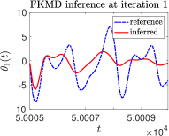
((a))

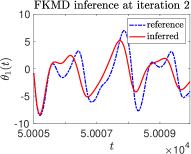
((b))

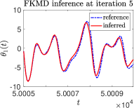
((c))

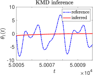
((d))

Figure 1: Comparison of FKMD with ordinary KMD for a $40$ dimensional Lorenz $96$ system, using random Fourier features. We predict the evolution of a single scalar observation, defined as the (mean-centered) first coordinate, $\theta_{1}(t)$, of the Lorenz system with nuisance variables. (a)-(c): FKMD at the $1$st, $2$nd and $5$th iterations, respectively. Results do not change much after $5$ iterations. (d): Ordinary KMD does not correlate with the data, even when nuisance coordinates are not included.

To illustrate the power of our method, we assume that we only observe $2.5\%$ of the system, namely the first coordinate $\theta_{1}$, and we add nuisance or “noise” variables. Specifically, we use the time embedding (9) with $\tau=0.05$ and

$$\bm{x}(n\tau)=\begin{bmatrix}\theta_{1}(n\tau)&\textup{noise}(n\tau)\end{bmatrix},$$ (16)

where $\textup{noise}(n\tau)$ for $n=0,1,2,\ldots$ are independent standard Gaussian random variables. To infer $\theta_{1}(t)$ from training data, we use Algorithm II.1 with random Fourier features defined in (14)-(15). Inference begins at the the end of the training set, and consists of $100$ discrete steps of time length $\tau$. The code for this experiment is available here.

For the FKMD parameters, we use $N=10^{6}$ sample points, $R=7500$ features, a time embedding of length $\ell=100$, and a constant bandwidth factor $h=1$. The observation $\bm{g}(\bm{x})$ is a $1\times 200$ vector associated with time embeddings of (16) as defined in (9). Results are plotted in Figure 1. If any one of $N$, $R$ or $\ell$ is decreased, results degrade noticeably. We use the top $20$ modes to define $\bm{M}$, as discussed in Appendix B, and we estimate $\sigma$ and $\bm{M}$ using a random subsample of $5000$ points. See Figure 2 for a visualization of $\bm{M}$.

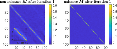
((a))

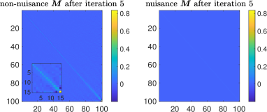
((b))

Figure 2: The Mahalanobis matrix $\bm{M}$ after the $1$st and $5$th iterations. To aid in visualization, we have split the matrix into nuisance coordinates at right and non-nuisance coordinates at left. (The insets at left are the bottom right $15\times 15$ submatrices of non-nuisance coordinates.) The matrix $\bm{M}$ maps away the nuisance coordinates, and finds appropriate structure in the non-nuisance coordinates.

Figure 1(a)-(c) shows inference using equation (8). On the $1$st iteration, the predictions collapse, but by the $5$th iteration, they are nearly a perfect match with the reference. The results do not change much after $5$ iterations. Figure 1(d) shows ordinary KMD. (Ordinary KMD corresponds to Algorithm II.1 with all the same parameters except the “second” time embedding $\ell=1$ is trivial, $\bm{M}$ is a scalar, iteration is unnecessary, and there are no nuisance variables.) In this experiment, ordinary KMD is not able to make good predictions.

The Mahalanobis matrices after the $1$st and $5$th iterations are shown in Figure 2(a)-(b). Here, we split $\bm{M}$ into nuisance and non-nuisance parts based on (16). Intuitively, the Mahalanobis matrix corresponds to a change of variables that eliminates the nuisance coordinates, while preserving the structure of the underlying signal, which here is $\theta_{1}(t)$.

III.2 Cell signaling dynamics

In a real-world data-driven setting, complex and potentially noisy temporal outputs derived from measurement may not obey a simple underlying ODE or live on a low-dimensional dynamical attractor. Information contained by internal signaling pathways within living cells is likely one such example, as it is both complex and subject to noisy temporal outputs arising from properties of the system itself and experimental sources.

With these considerations in mind, we next apply our method to dynamic signaling activity in cancer cells to assess its performance. Here we show that our methods enable the forward prediction of single-cell signaling activity from past knowledge in a system where signaling is highly variable from cell-to-cell and over timeDavies et al. (2020). The extracellular signal-regulated kinases (ERK) signaling pathway is critical for perception of cues outside of cells, and for translation of these cues into cellular behaviors such as changes in cell shape, proliferation rate, and phenotypeCopperman et al. (2023). Dynamic ERK activity is monitored via the nuclear or cytoplasmic localization of the fluorescent reporter (Figure 3A). We track single-cells through time in the live-cell imaging yielding single-cell ERK activity time series (Figure 3C). The first 72 hours of single-cell trajectories serve as the training set to estimate the Koopman operator, and we withhold the final 18 hours of the single-cell trajectories to test the forward predictive capability. The raw ERK activity trajectories on their own yield no predictive capability via standard Kernel DMD methods, but our iterative procedure to extract the Mahalanobis matrix leads to a coordinate rescaling which couples signaling activity across delay times (Figure 3B,D) and enables a forward prediction of ERK activity across the testing window (Figure 3D).

We use $N=5202$ samples and kernel features with $R=N$, and we choose bandwidth $h=1.05$ and a time embedding of length $\ell=49$. The function $\bm{g}(\bm{x})$ is a $1\times 49$ time embedding of the scalar ERK activity. For inference, we exclude modes where $\textup{Re}(\lambda_{m})>0.15$ and $|\textup{Im}(\lambda_{m})|>\pi/3$; see Appendix A. This amounts to excluding unstable modes and modes that oscillate quickly. We use the top few modes to construct $\bm{M}$, as discussed in Appendix B. Inference begins immediately after the end of the training set. Forward prediction performance is quantified by estimating the relative error and correlation between inferred and test set ERK activity trajectories.

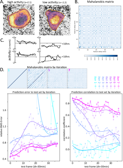
Figure 3: FKMD enabled cell signaling state prediction. (a) Fluorescent ERK reporter expressing breast cancer cell embedded in a mammary tissue organoid, showing representative high activity (left, cytoplasmic localized) and low activity (right, nucleus localized). (b) Malahanobis matrix at iteration 8, where test set correlation is maximized. (c) Representative single-cell ERK activity traces, measured test set (solid lines) and FKMD-predicted (dashed lines). (d) Mahalanobis matrix by FKMD iteration (top), and FKMD prediction performance from 0-18hrs quantified by relative RMS error and correlation to test set (bottom left and right) by iteration number (cyan to magenta circles), solid lines are spline fits added as guides to the eye.

IV Discussion and future work

This article introduces FKMD, a method we have proposed to featurize Koopman Mode Decomposition that generates more accurate predictions than standard (e.g., Gaussian kernel) KMD. By modeling data assuming uniform changes in space and time, our Mahalanobis scaling helps mitigate the curse of dimensionality. Results in two separate application areas – climate and cell signaling dynamics – illustrate the promise of the method for inferring future states of time series generated by complex systems.

Many theoretical and algorithmic questions remain. We would like to better understand parameter choices, particularly how to choose modes for the Mahalanobis matrix computation, as described in Appendix B, and how many iterations to run. Empirically, we have found that a few iterations and modes lead to good results, but more empirical testing is needed, and our theoretical understanding of these issues is lacking. For example, we cannot yet describe a simple set of conditions that guarantees good behavior of Algorithm II.1, e.g., convergence to a fixed point.

We would also like to explore alternative methods for scaling up our methods to larger sample sizes. Here, we use random Fourier features to scale up FKMD, but more analysis and comparison with alternative methods are still needed. Another possible trick to increase sample size may come from modern advances in randomized numerical linear agebra, e.g. randomly pivoted Cholesky Tropp and Webber (2023); Chen et al. (2022). Such methods promise spectral efficiency for solving symmetric positive definite linear systems. Assuming fast spectral decay of $\bm{\Psi}_{\bm{x}}$ (which we have observed empirically), these techniques could help our methods scale to even larger sample sizes. We will explore application of these cutting-edge methods in future works.

Finally, we would like to better understand mechanisms, i.e., what makes a system head towards a certain state $B$ rather than another state $A$? These states could be associated with El Niño occurring or not, or with cancer remaining in a cell or spreading. This can be formalized by the concept of the committor, the probability that the system reaches state $B$ before $A$, starting at point $\bm{x}$. By imposing appropriate boundary conditions on the data, the committor can be represented as a Koopman eigenfunction associated to eigenvalue $1$. This suggests a particular choice of $\bm{M}$ based on using only this mode. In this case, $\bm{M}$ could potentially identify what directions are associated with important mechanisms leading to $A$ or $B$. We hope to explore this idea in future work.

Appendix A Derivation of Koopman eigendecomposition

Here, we show how to arrive at the Koopman eigendecomposition (8). This has been shown already in Williams et al. (2015), but we provide a streamlined derivation here for convenience.

Recall that the matrix $\bm{K}$ is a finite dimensional approximation to the Koopman operator. This approximation is obtained by applying a change of variables from sample space to feature space. The change of variables is given by the matrix $\bm{\Psi}_{\bm{x}}$. This leads to the following equation for inference:

$$\begin{bmatrix}\mathcal{K}_{\tau}(\bm{g})(\bm{x}_{1})\\ \vdots\\ \mathcal{K}_{\tau}(\bm{g})(\bm{x}_{N})\end{bmatrix}\approx\bm{\Psi}_{\bm{x}}\bm{K}\bm{\Psi}_{\bm{x}}^{{\dagger}}\begin{bmatrix}\bm{g}(\bm{x}_{1})\\ \vdots\\ \bm{g}(\bm{x}_{N})\end{bmatrix},$$ (17)

where ${\dagger}$ denotes the Moore-Penrose pseudoinverse. Similarly,

$$\bm{B}=\bm{\Psi}_{\bm{x}}^{{\dagger}}\begin{bmatrix}\bm{g}(\bm{x}_{1})\\ \vdots\\ \bm{g}(\bm{x}_{N})\end{bmatrix}.$$

The eigendecomposition of $\bm{K}$ can be written as

$$\bm{K}=\bm{\Xi}\bm{D}\bm{W}^{\ast},$$ (18)

where $\bm{K}\bm{\Xi}=\bm{\Xi}\bm{D}$ and $\bm{W}^{\ast}\bm{K}=\bm{D}\bm{W}^{\ast}$, and we may assume that $\bm{W}^{\ast}\bm{\Xi}=\bm{I}$. Here, $\bm{D}$ is the diagonal matrix of Koopman eigenvalues, $\mu_{m}$; that is, $\bm{D}=\exp(\tau\bm{\Lambda})$ where $\bm{\Lambda}$ is the diagonal matrix of continuous time Koopman eigenvalues, $\lambda_{m}$.

Plugging (18) into (17),

$$\begin{bmatrix}\mathcal{K}_{\tau}(\bm{g})(\bm{x}_{1})\\ \vdots\\ \mathcal{K}_{\tau}(\bm{g})(\bm{x}_{N})\end{bmatrix}\approx\bm{\Psi}_{\bm{x}}\bm{\Xi}\exp(\tau\bm{\Lambda})\bm{W}^{\ast}\bm{B}.$$ (19)

The definition of Koopman modes and Koopman eigenfunctions shows that the rows of $\bm{W}^{\ast}\bm{B}$ are the Koopman modes $\bm{v}_{m}^{\ast}$, while the Koopman eigenfunctions are sampled by the columns of

$$\bm{\Psi}_{\bm{x}}\bm{\Xi}=\begin{bmatrix}\phi_{1}(\bm{x}_{1})&\ldots&\phi_{R}(\bm{x}_{1})\\ \vdots&&\vdots\\ \phi_{1}(\bm{x}_{N})&\ldots&\phi_{R}(\bm{x}_{N})\end{bmatrix}.$$ (20)

Substituting (20) into (19) and writing the matrix multiplication in terms of outerproducts yields equation (8), provided we substitute $\bm{x}_{n}$ for $\bm{x}$, using any sample point $\bm{x}_{n}$.

Note that equation (8) naturally allows for mode selection. For example, modes that lead to predictions that are a priori known to be unphysical, e.g. diverging modes associated to eigenvalues with $\textup{Re}(\lambda_{m})\gg 0$, can simply be omitted from the sum in (8). Similar selection can be done to remove modes that oscillate too fast, i.e., $|\textup{Im}(\lambda_{m})|\gg 0$. We have done this in the experiments in Section III.2.

Appendix B Choice of Mahalanobis matrix

Here, we explain the reasoning behind the choice of Mahalanobis matrix. Notice that our kernels have the form

$$k_{\bm{M}}(\bm{x},\bm{x}^{\prime})=\exp\left(-\|\bm{x}-\bm{x}^{\prime}\|_{\bm{M}}^{2}\right),\quad\|\bm{x}\|_{\bm{M}}^{2}:=\bm{x}^{\ast}\bm{M}\bm{x}.$$

In addition, $\|\bm{x}\|_{\bm{M}}=\|\bm{M}^{1/2}\bm{x}\|$, where the second norm is the usual Euclidean one. The Mahalanobis scaling can then be interpreted as just a change of variables, $\tilde{\bm{x}}=\bm{M}^{1/2}\bm{x}$, where the tilde notation indicates the changed variables.

Below, we use tildes to denote the changed variables, $\tilde{\bm{x}}=\bm{M}^{1/2}\bm{x}$, and write $\tilde{\bm{g}}(\tilde{\bm{x}})=\bm{g}(\bm{x})$ for $\bm{g}$ in these changed variables. We will implicitly assume appropriate smoothness so that all the derivatives calculations below make sense. Also, we will assume that $\bm{M}$ is invertible.

Proposition B.1.

Define a function $f$ on unit vectors $\bm{u}$ by

$$f(\bm{u})=\frac{1}{N}\sum_{n=1}^{N}\left|\bm{u}^{\ast}\tilde{\bm{J}}(\tilde{\bm{x}}_{n})\right|^{2}.$$ (21)

where $\tilde{\bm{J}}$ is given by

$$\tilde{\bm{J}}(\tilde{\bm{x}}_{n})=\lim_{\tau\to 0}\tau^{-1}[\nabla\tilde{\bm{g}}(\tilde{\bm{y}}_{n})-\nabla\tilde{\bm{g}}(\tilde{\bm{x}}_{n})].$$

In the idealized case of zero Koopman estimation error, i.e., equality in (8), the function $f$ is constant valued.

Proof.

Assuming no estimation error,  (8) and (13) imply

$$\begin{split}\bm{J}(\bm{x}_{n})&=\nabla\left(\left.\frac{d}{dt}\mathcal{K}_{\tau}\bm{g}(\bm{x}_{n})\right|_{\tau=0}\right)\\ &=\lim_{\tau\to 0}\tau^{-1}[\nabla\bm{g}(\bm{y}_{n})-\nabla\bm{g}(\bm{x}_{n})].\end{split}$$ (22)

By the chain rule, $\nabla\tilde{\bm{g}}(\tilde{\bm{x}}_{n})=\bm{M}^{-1/2}\nabla\bm{g}(\bm{x}_{n})$. Thus,

$$f(\bm{u}) =\frac{1}{N}\sum_{n=1}^{N}\left|\bm{u}^{\ast}\bm{M}^{-1/2}\bm{J}(\bm{x}_{n})\right|^{2}$$

$$=\frac{1}{N}\sum_{n=1}^{N}\bm{u}^{\ast}\bm{M}^{-1/2}\bm{J}(\bm{x}_{n})\bm{J}(\bm{x}_{n})^{\ast}\bm{M}^{-1/2}\bm{u}$$

$$=\frac{1}{N}(h\sigma)^{2},$$

where $\bm{M}$ is defined by (12) and Step 1 of Algorithm II.1. ∎

We interpret $\bm{J}$ and $\tilde{\bm{J}}$ as a kind of dynamical curvature in the original and transformed variables. See Remark B.2 for intuition behind this term. We have shown that the average inner product between any test vector $\bm{u}$ and the dynamical curvature at each point is constant. This implies that we have constant average dynamical curvature in all directions. We have loosely referred to this property as “uniform changes in space and time.”

Remark B.2.

Suppose that $\mathcal{F}_{\tau}$ is the evolution map of a linear ODE driven by a real invertible matrix $\bm{A}$,

$$\frac{d\bm{x}(t)^{\ast}}{dt}=\bm{x}(t)^{\ast}\bm{A},$$

and that the observation function records the whole state, $\bm{g}(\bm{x})=\bm{x}^{\ast}$. In this case, $\bm{J}=\bm{A}$ and $\bm{M}=\bm{A}\bm{A}^{\ast}$, while

$$\tilde{\bm{J}}=(\bm{A}\bm{A}^{\ast})^{-1/2}\bm{A}$$

is an orthogonal matrix. Here, $\bm{J}$ and $\tilde{\bm{J}}$ represent curvature in the original and changed variables, respectively; in particular, the variable change makes the evolution appear to be driven by $\tilde{\bm{J}}$ rather than ${\bm{J}}=\bm{A}$.

This explains the choice of $\bm{M}$ except for the variable scalar bandwidth $\sigma$. Computing $\sigma$ from standard deviations of pairwise distances is standard, except that in Algorithm II.1 it is applied to the transformed samples, $\bm{M}^{1/2}\bm{x}$, to appropriately reflect the change of variables. The additional constant scaling factor $h$ can be chosen using standard techniques such as cross validation Nüske et al. (2023).

We have noticed empirically that estimates of $\bm{M}$ can suffer from noise effects if too many modes are used. In particular, we find good results by using only top modes according to some cutoff in (13); e.g., removing modes with $\textup{Re}(\lambda_{m})<-\gamma$, where $\gamma>0$ is some threshold. Intuitively, this means eliminating effects from the shortest timescales. We use this idea in the experiments in Section III.1 and Section III.2.

Remark B.3.

It is intuitively reasonable to consider using

$$\bm{J}(\bm{x}):=\left(\left.\frac{d}{dt}\mathcal{K}_{t}\bm{g}(\bm{x})\right|_{t=0}\right)^{\ast},$$ (23)

where $\bm{g}(\bm{x})=\bm{x}^{\ast}$ observes the full sample. Empirically, we find that equation (22) outperforms (23). Another advantage of (22) is that it is tailored to a particular observation function, while (23) requires reconstructing the full sample.

Appendix C Connection between kernel and random Fourier features

The connection between the kernel features (10)- (11) and random Fourier features (14)- (15) is the following.

Proposition C.1.

We have

$$k_{\bm{M}}(\bm{x},\bm{x}^{\prime})={\bf E}\left[\psi_{m}^{RFF}(\bm{x})^{\ast}\psi_{m}^{RFF}(\bm{x}^{\prime})\right]$$

where ${\bf E}$ denotes expected value.

Proof.

Since $\bm{M}$ is Hermitian,

$$\|\bm{x}\|_{\bm{M}}=\|\bm{x}\|_{\textup{Re}(\bm{M})}$$

for real $\bm{x}$. Because of this we may, without loss of generality, assume that $\bm{M}$ is real. Let $\bm{\delta}=\bm{x}^{\prime}-\bm{x}$ and $\tilde{\bm{\delta}}=\bm{M}^{1/2}\bm{\delta}$. By completing the square,

$$-\frac{1}{2}|\bm{\omega}|^{2}+i\bm{\omega}^{T}\bm{M}^{1/2}\delta=-\frac{1}{2}\left[(\bm{\omega}-i\tilde{\bm{\delta}})^{T}(\bm{\omega}-i\tilde{\bm{\delta}})\right]-\frac{1}{2}|\tilde{\bm{\delta}}|^{2},$$

so if samples live in $d$-dimensional (real) space, we get

$${\bf E}\left[\psi_{m}^{RFF}(\bm{x})^{\ast}\psi_{m}^{RFF}(\bm{x}^{\prime})\right]$$

$$=(2\pi)^{-d/2}\int\exp(-|\bm{\omega}|^{2})\exp(i\bm{\omega}^{T}\bm{M}^{1/2}\bm{\delta})\,d\bm{\omega}$$

$$=\exp(-|\tilde{\delta}|^{2}/2)=k_{\bm{M}}(\bm{x},\bm{x}^{\prime}).$$

∎

Based on Proposition C.1, we now show the connection between FKMD procedures with kernel and random Fourier features. Let $\bm{\Psi}_{\bm{x}}^{RFF}$ and $\bm{\Psi}_{\bm{y}}^{RFF}$ be the $N\times R$ samples by features matrices associated to random Fourier features (14), and let $\bm{\Psi}_{\bm{x}}$ and $\bm{\Psi}_{\bm{y}}$ be the same matrices associated with kernel features (10). Using Proposition C.1, for large $R$ we have

$$\bm{\Psi}_{\bm{x}}\approx\bm{\Psi}_{\bm{x}}^{RFF}(\bm{\Psi}_{\bm{x}}^{RFF})^{\ast},\qquad\bm{\Psi}_{\bm{y}}\approx\bm{\Psi}_{\bm{y}}^{RFF}(\bm{\Psi}_{\bm{x}}^{RFF})^{\ast}.$$ (24)

Assume the columns of $\bm{\Psi}_{\bm{x}}^{RFF}$ are linearly independent. Then

$$(\bm{\Psi}_{\bm{x}}^{RFF})^{\ast}[(\bm{\Psi}_{\bm{x}}^{RFF})^{\ast}]^{\dagger}=\bm{I}$$ (25)

where ${\dagger}$ is the Moore-Penrose pseudoinverse. Define

$$\bm{K}^{RFF}=(\bm{\Psi}_{\bm{x}}^{RFF})^{\ast}\bm{K}[(\bm{\Psi}_{\bm{x}}^{RFF})^{\ast}]^{\dagger},$$ (26)

where $\bm{K}$ satisfies

$$\bm{\Psi}_{\bm{x}}\bm{K}=\bm{\Psi}_{\bm{y}}.$$ (27)

Multiplying (27) by $(\bm{\Psi}_{\bm{x}}^{RFF})^{\ast}$ and $[(\bm{\Psi}_{\bm{x}}^{RFF})^{\ast}]^{\dagger}$ on the left and right, and then using (24)-(26), leads to

$$(\bm{\Psi}_{\bm{x}}^{RFF})^{\ast}\bm{\Psi}_{\bm{x}}^{RFF}\bm{K}^{RFF}\approx(\bm{\Psi}_{\bm{x}}^{RFF})^{\ast}\bm{\Psi}_{\bm{y}}^{RFF},$$

which is the least squares normal equation for

$$\bm{\Psi}_{\bm{x}}^{RFF}\bm{K}^{RFF}=\bm{\Psi}_{\bm{y}}^{RFF}.$$ (28)

This directly connects the linear solves (27) and (28) for the Koopman matrix using kernel and random Fourier features, respectively. Moreover, from (24)-(26),

$$\begin{split}\bm{\Psi}_{\bm{x}}^{RFF}\bm{K}^{RFF}(\bm{\Psi}_{\bm{x}}^{RFF})^{\dagger}\approx\bm{\Psi}_{\bm{x}}\bm{K}\bm{\Psi}_{\bm{x}}^{\dagger}.\end{split}$$ (29)

In light of (17), equation (29) shows that Fourier features and kernel features give (nearly) the same equation for inference.

Due to Proposition C.1 and the computations in (24)-(29) above, random Fourier features (14) and kernel features (10) target essentially the same FKMD procedure whenever $R$ is sufficiently large. In practice this means random Fourier features can be a more efficient way of solving the same problem.

Data generation

ERK activity reporters, cell line generation, and live-cell imaging have been described in detail in Davies et al Davies et al. (2020). Here we utilize a dataset monitoring ERK activity in tissue-like 3D extracellular matrix. Images were collected every 30 minutes over a 90-hour window. Single-cells were segmented using Cellpose software Pachitariu and Stringer (2022) and tracked through time by matching cells to their closest counterpart at the previous timepoint. ERK reporter localization was monitored via the mean-centered and variance stabilized cross-correlation between the nuclear reporter and ERK activity reporter channels in the single-cell cytoplasmic mask. Single-cell trajectories up to 72 hours served as the training set to estimate the Koopman operator.

References

- Mezić (2005) I. Mezić, Nonlinear Dynamics 41, 309 (2005).
- Mezić (2021) I. Mezić, Not. Am. Math. Soc. 68, 1087 (2021).
- Koopman (1931) B. O. Koopman, Proceedings of the National Academy of Sciences 17, 315 (1931).
- Koopman (2004) J. Koopman, Annu. Rev. Public Health 25, 303 (2004).
- Williams et al. (2015) M. O. Williams, I. G. Kevrekidis, and C. W. Rowley, Journal of Nonlinear Science 25, 1307 (2015).
- Tu (2013) J. H. Tu, Dynamic mode decomposition: Theory and applications, Ph.D. thesis, Princeton University (2013).
- Kevrekidis et al. (2016) I. Kevrekidis, C. W. Rowley, and M. Williams, Journal of Computational Dynamics 2, 247 (2016).
- Proctor et al. (2016) J. L. Proctor, S. L. Brunton, and J. N. Kutz, SIAM Journal on Applied Dynamical Systems 15, 142 (2016).
- Kawashima and Hino (2022) T. Kawashima and H. Hino, Neural Computation 35, 82 (2022).
- Baddoo et al. (2023) P. J. Baddoo, B. Herrmann, B. J. McKeon, J. Nathan Kutz, and S. L. Brunton, Proceedings of the Royal Society A 479, 20220576 (2023).
- Mezić (2013) I. Mezić, Annual review of fluid mechanics 45, 357 (2013).
- Bagheri (2013) S. Bagheri, Journal of Fluid Mechanics 726, 596 (2013).
- Arbabi and Mezić (2017) H. Arbabi and I. Mezić, Physical Review Fluids 2, 124402 (2017).
- Wu et al. (2017) H. Wu, F. Nüske, F. Paul, S. Klus, P. Koltai, and F. Noé, The Journal of chemical physics 146 (2017).
- Klus et al. (2020a) S. Klus, F. Nüske, S. Peitz, J.-H. Niemann, C. Clementi, and C. Schütte, Physica D: Nonlinear Phenomena 406, 132416 (2020a).
- Navarra et al. (2021) A. Navarra, J. Tribbia, and S. Klus, Journal of the Atmospheric Sciences 78, 1227 (2021).
- Rahimi and Recht (2007) A. Rahimi and B. Recht, Advances in neural information processing systems 20 (2007).
- Nüske and Klus (2023) F. Nüske and S. Klus, arXiv preprint arXiv:2306.00849 (2023).
- Lorenz (1996) E. N. Lorenz, in Proc. Seminar on predictability, Vol. 1 (Reading, 1996).
- Brunton et al. (2021) S. L. Brunton, M. Budišić, E. Kaiser, and J. N. Kutz, arXiv preprint arXiv:2102.12086 (2021).
- Mauroy et al. (2020) A. Mauroy, Y. Susuki, and I. Mezić, Koopman operator in systems and control (Springer, 2020).
- Bishop and Nasrabadi (2006) C. M. Bishop and N. M. Nasrabadi, Pattern recognition and machine learning, Vol. 4 (Springer, 2006).
- Arbabi and Mezic (2017) H. Arbabi and I. Mezic, SIAM Journal on Applied Dynamical Systems 16, 2096 (2017).
- Baddoo et al. (2022) P. J. Baddoo, B. Herrmann, B. J. McKeon, and S. L. Brunton, Proceedings of the Royal Society A 478, 20210830 (2022).
- Nüske et al. (2023) F. Nüske, S. Peitz, F. Philipp, M. Schaller, and K. Worthmann, Journal of Nonlinear Science 33, 14 (2023).
- Klus et al. (2020b) S. Klus, F. Nüske, and B. Hamzi, Entropy 22, 722 (2020b).
- Takens (2006) F. Takens, in Dynamical Systems and Turbulence, Warwick 1980: proceedings of a symposium held at the University of Warwick 1979/80 (Springer, 2006) pp. 366–381.
- Kamb et al. (2020) M. Kamb, E. Kaiser, S. L. Brunton, and J. N. Kutz, SIAM Journal on Applied Dynamical Systems 19, 886 (2020).
- Radhakrishnan et al. (2022) A. Radhakrishnan, D. Beaglehole, P. Pandit, and M. Belkin, arXiv preprint arXiv:2212.13881 (2022).
- Li (1991) K.-C. Li, Journal of the American Statistical Association 86, 316 (1991).
- Trivedi et al. (2014) S. Trivedi, J. Wang, S. Kpotufe, and G. Shakhnarovich, in UAI (2014) pp. 819–828.
- Yamashita et al. (2018) R. Yamashita, M. Nishio, R. K. G. Do, and K. Togashi, Insights into imaging 9, 611 (2018).
- Khanna (1990) T. Khanna, Foundations of neural networks (Addison-Wesley Longman Publishing Co., Inc., 1990).
- Freeman and Skapura (1991) J. A. Freeman and D. M. Skapura, Neural networks: algorithms, applications, and programming techniques (Addison Wesley Longman Publishing Co., Inc., 1991).
- Cheng and Titterington (1994) B. Cheng and D. M. Titterington, Statistical science , 2 (1994).
- Tropp and Webber (2023) J. A. Tropp and R. J. Webber, arXiv preprint arXiv:2306.12418 (2023).
- Yang et al. (2012) T. Yang, Y.-F. Li, M. Mahdavi, R. Jin, and Z.-H. Zhou, Advances in neural information processing systems 25 (2012).
- Kammonen et al. (2020) A. Kammonen, J. Kiessling, P. Plecháč, M. Sandberg, and A. Szepessy, arXiv preprint arXiv:2007.10683 (2020).
- Lorenz (1963) E. N. Lorenz, Journal of atmospheric sciences 20, 130 (1963).
- Hu and Van Leeuwen (2021) C.-C. Hu and P. J. Van Leeuwen, Quarterly Journal of the Royal Meteorological Society 147, 2352 (2021).
- Butcher (1996) J. C. Butcher, Applied numerical mathematics 20, 247 (1996).
- Note (1) https://github.com/davidaristoff/FKMD/tree/main.
- Davies et al. (2020) A. E. Davies, M. Pargett, S. Siebert, T. E. Gillies, Y. Choi, S. J. Tobin, A. R. Ram, V. Murthy, C. Juliano, G. Quon, et al., Cell systems 11, 161 (2020).
- Copperman et al. (2023) J. Copperman, S. M. Gross, Y. H. Chang, L. M. Heiser, and D. M. Zuckerman, Communications Biology 6, 484 (2023).
- Chen et al. (2022) Y. Chen, E. N. Epperly, J. A. Tropp, and R. J. Webber, arXiv preprint arXiv:2207.06503 (2022).
- Pachitariu and Stringer (2022) M. Pachitariu and C. Stringer, Nature methods 19, 1634 (2022).
- Christensen and Von Lilienfeld (2020) A. S. Christensen and O. A. Von Lilienfeld, Machine Learning: Science and Technology 1, 045018 (2020).
- Kanagawa et al. (2018) M. Kanagawa, P. Hennig, D. Sejdinovic, and B. K. Sriperumbudur, arXiv preprint arXiv:1807.02582 (2018).
- Lin et al. (2023) Y. T. Lin, Y. Tian, D. Perez, and D. Livescu, SIAM Journal on Applied Dynamical Systems 22, 2890 (2023).
- Rayner et al. (2003) N. Rayner, D. E. Parker, E. Horton, C. K. Folland, L. V. Alexander, D. Rowell, E. C. Kent, and A. Kaplan, Journal of Geophysical Research: Atmospheres 108 (2003).