Measurement-induced landscape transitions in hybrid variational quantum circuits

Abstract

The entanglement-induced “barren plateau” phenomenon is an exponential vanishing of the parameter gradients with system size that limits the use of variational quantum algorithms(VQA). Recently, it was observed that a “landscape” transition from a barren plateau to no barren plateau occurs if the volume-law growth of entanglement is suppressed by adding measurements with post-selection[1]. This suppression appears to coincide with a measurement-induced phase transition (MIPT) that measurements are known to cause in monitored circuits[2, 3, 4]. From an information theory perspective, we argue that these are different transitions. We back this hypothesis with a numerical study of the cost landscape of such hybrid variational quantum circuits with extensive results on the behavior of cost-gradient variances with and without post-selection, direct visualizations of optimization runs for specific local quantum circuits, and a mutual information measure we introduce and compare with entanglement measures used in the study of MIPT. Specifically, our results show there are two transitions, a measurement-induced landscape transition (MILT) that seems universal across different VQA ansatzes and appears at a lower probability of measurements, and the MIPT that appears at a higher probability of measurements and appears at an ansatz specific location. Finally, to reap the benefits of MILT for optimization, our numerical simulations suggest the necessity of post-selecting measurement outcomes.

1 Introduction

The age of noisy intermediate-scale quantum devices (NISQ) has seen the advent of quantum computers and simulators with nearly hundreds of qubits, noisy yet capable of serious computation [5]. Although the long-term goal in quantum computing is to build error-corrected qubits, current noisy qubits still promise a potential quantum advantage. Variational quantum algorithms (VQA) have been central to much of the efforts in this direction [6, 7, 8]. VQA refers to the class of hybrid quantum-classical algorithms based on training parameterized quantum circuits by using a classical optimizer. They are desirable especially for the NISQ hardware because of their low depth.

Practical implementation of the VQAs comes with its challenges—most prominently, the tradeoff between expressibility vs. trainability of the circuit. The success of a VQA depends on the expressibility of the variational ansatz under consideration, i.e., the ansatz must be able to approximate the solution with reasonable accuracy [9, 10, 11]. Nevertheless, strong expressibility leads to poor trainability due to cost landscapes, a phenomenon dubbed barren plateaus (BP) [12, 13, 14, 15, 11]. Characterized by the exponential vanishing of the gradient’s variance with the system size, BP typically arise in circuits deep enough to form a 2-design [12]. Thus, it poses a severe bottleneck in the scalability of the VQAs and their ability to solve complex problems.

Numerous strategies have been proposed to mitigate barren plateaus. These include problem-inspired [16] and adaptive ansatz [17] , local cost function[13], pre-training[18], identity-block initialization[19], etc. Some recent studies have focused on the relationship between entanglement growth in random circuits and the onset of barren plateaus [15, 20, 21]. Computing the many-body entanglement during the training process can be helpful to avoid BP via control of learning rate[21]. Nevertheless, the strategies proposed so far are either ad-hoc or increase the depth of the circuit, so we are still far from solving the BP problem.

Recently, it was observed that a “landscape” transition can occur if measurements are added to a VQA ansatz[1]. Without measurements, the entanglement entropy of a quantum chain undergoing local unitary evolution grows linearly in time until it thermalizes to a volume-law entangled state[22]. In contrast, local measurements tend to disentangle the system via wavefunction collapse. A dynamical competition between these two circuit components leads to a phase transition between phases with different system size scaling of entanglement in a variety of models, a topic of wide interest in recent years dubbed the measurement-induced phase transition (MIPT)[2, 3, 4, 23, 24, 25, 26]. This “purification dynamics” [27] suggests we can control entanglement and the BP with measurements and supports the observation of a landscape transition that appears to coincide with the MIPT[1].

In this manuscript, we argue the MIPT and the landscape transition are different phase transitions on information theoretic grounds. We support this hypothesis with extensive numerical evidence on cost function gradient variances, landscape visualizations, and information-theoretic measures. We observe that this measurement-induced landscape transition (MILT) appears seemingly at a universal critical measurement probability rate across different ansatzes, at a lower rate than the MIPT and does not require post-selection to identify. Yet we find that projective measurements and post-selection can be exploited to assist optimization.

1.1 Information theory of optimization

There is an information-theoretic way to understand quantum optimization. In principle, the problem is straightforward. One parameterizes a space of wave functions $|\psi({\bm{\theta}})\rangle$, with ${\bm{\theta}}$ a multidimensional array of real numbers. Then, by choosing initial values for ${\bm{\theta}}$, and quantum computing the gradient of the cost function $\langle\psi({\bm{\theta}})|\hat{O}|\psi({\bm{\theta}})\rangle$, one takes small steps down-hill in the cost landscape until reaching a local minimum. But we can turn this around, as in Fig. 1, and view it as a communication problem.

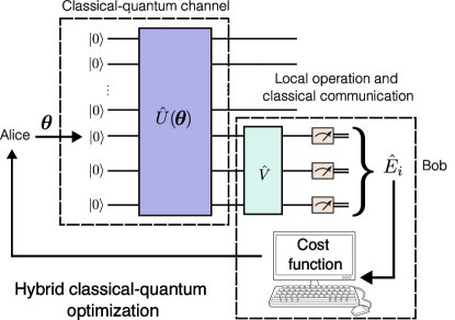
Figure 1: An information theory perspective of optimization in two steps. Alice draws parameters from $p_{A}({\bm{\theta}})$, and sends copies of them to Bob via a classical-quantum channel ${\bm{\theta}}\mapsto\hat{\rho}_{\bm{\theta}}$. Bob then performs measurements $\{\hat{E}_{i}\}$ on $\hat{\rho}_{\bm{\theta}}$, computes the expectation value of the cost operator $\hat{O}$, and sends the results back to Alice, which amounts to a local operation and classical communication (LOCC).

Suppose Alice is the person responsible for choosing the parameters. Alice chooses a parameter ${\bm{\theta}}$ from a classical distribution $p_{A}({\bm{\theta}})$ and sends many copies of it to Bob via a classical-quantum channel $\mathcal{N}:{\bm{\theta}}\mapsto\hat{\rho}_{{\bm{\theta}}}$ (see chapter 5 of Holevo[28] for a definition of classical-quantum channels). Bob has access to these quantum states via POVM measurements $\{\hat{E}_{i}\}$ associated with the eigenbases of the to-be-optimized observable $\hat{O}$ with which he tries to decode the classical information sent by Alice. Between Alice’s choices of parameters and these measurement outcomes is therefore a classical information channel

$$p(x\mid{\bm{\theta}})=\Tr[\hat{\rho}_{\bm{\theta}}\hat{E}_{i}].$$ (1)

Finally, the measurement outcomes are used to compute the cost function, a computation whose results are sent back to Alice via a (noiseless) classical communication channel. The steps between Bob’s local measurements and sending the results back to Alice constitute a local operation and classical communication (LOCC).

If any intermediate measurements occur in the circuit, we consider both cases where the measurement outcomes may or may not be available to Bob. If the measurements are available to Bob, then the classical-quantum channel becomes ${\bm{\theta}}\mapsto\ \hat{\rho}_{{\bm{\theta}},m}$ where $\hat{\rho}_{{\bm{\theta}},m}$ is the quantum state formed from the collapse of the wave function. Otherwise, the channel remains the same as above, but the state $\rho_{\bm{\theta}}$ has thermalized.

This information theory perspective allows us to illustrate the measurement-induced landscape transition. If no measurements take place, the classical-quantum channel ${\bm{\theta}}\mapsto\rho_{\bm{\theta}}$ encodes Alice’s classical information into a highly entangled state, making it difficult for Bob to decode from Bob’s local measurements $\{\hat{E}_{i}\}$. This difficulty is the cause of the BP[12]. Based on this intuition, BP should be accompanied by an exponential reduction of the channel’s capacity to transmit information between Alice and Bob. If many intermediate measurements are performed, and these measurement outcomes are known to Bob, then a quantum zeno effect takes place[2]. The many measurements render the state $\hat{\rho}_{{\bm{\theta}},m}$ largely independent of earlier parameters ${\bm{\theta}}$ but the state no longer has a high degree of entanglement. If the measurement outcomes are unknown to Bob, then the thermalization of $\hat{\rho}_{\bm{\theta}}$ takes place and introduces significant noise. These phenomena have different system size scaling, so we expect a phase transition between them. Thus, one can hope for an optimal trade-off between no measurements and many measurements, perhaps at a critical point between the two, where optimization is substantially improved.

We can contrast this information-theoretic view of optimization with that of the MIPT[27, 26]. In a MIPT, Alice chooses a quantum state $\rho$ and sends this to Bob via a quantum channel $\hat{\rho}\mapsto\hat{\rho}^{\prime}$. Bob then needs to decode the quantum information sent by Alice with knowledge of any measurement outcomes that took place in the channel, and Bob typically measures the entanglement of the state to identify the phase transition, a resource not available in optimization. The challenge of detecting a MIPT is therefore different from that of identifying MILT.

1.2 Optimization problems and post-selection

The goal of finding the desired ground state in the space of an exponentially large Hilbert space is an arduous task. An ideal variational ansatz capable of achieving it must be able to create a complex network of entanglement between the qubits, yet explore only a polynomial-sized space near the solution point. But such expressibility often comes at the price of more variational parameters and a landscape plagued with BPs and narrow gorges [13].

We need to choose several ansatzes to capture the typical behavior of landscape transitions and their information-theoretic properties. Since the building blocks of any variational ansatz are single qubit rotations and entangling gates we can choose these gates and the connectivity between the qubits to match the device architecture and obtain a hardware efficient ansatz (HEA)[29]. Although flexible and highly expressible, optimizing them for a specific problem can be challenging in practice. Thus, it is often useful to turn to problem-inspired ansatzes, for example, quantum approximate optimization algorithm  (QAOA)[30] for combinatorial optimization problems and Hamiltonian variational ansatz  (HVA)[31, 32] for finding the ground state. For problems involving long length scales, renormalization group-like flows can be implemented with the quantum convolutional neural network (QCNN)[33], found to be free from BP [34]. For certain problems, one may also choose how the various building blocks in the circuits are stacked. An example of this paradigm is the ADAPT-VQE algorithm [35, 36], which is also BP-free [17]. Our work is inspired by the quest to improve existing ansatzes by introducing measurement gates which allows control over the growth of entanglement in the circuit.

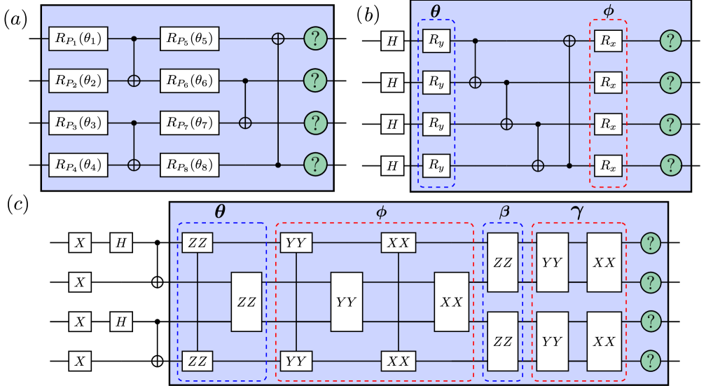
Figure 2: A diagram depicting a single layer of the 4-qubit version of the ansatzes examined in this paper. Each ansatz can be generalized to other even number of qubits. The blue shaded regions in each diagram are those repeated in every layer, whereas those outside of it are used only for the initial layer. Measurement gates, represented by the green circles, are randomly placed with probability $p$ after each layer except the last. (a) HEA1: Apply a $R_{P_{i}}$ gate to each qubit, followed by CNOT pairs on even paired qubits, followed by applying more $R_{P_{i}}$ gates to each qubit, followed by applying CNOT pairs to odd paired qubits. Each $R_{P_{i}}$ gate represents a randomly rotation gate generated by a Pauli operator $P_{i}$, paramaterized by an angle ${\bm{\theta}}_{i}$. (b) HEA2 and (c) XXZ-HVA are heavily inspired by the ansatzes used in Wiersama et al [1]. Note that the parameters are applied uniformly across all the qubits in (b) and (c).

We focus specifically on the following three ansatzes:

1. Hardware efficient ansatz 1 (HEA1)

2. Hardware efficient ansatz 2 (HEA2)

3. XXZ Hamiltonian variational ansatz (XXZ-HVA)

The ansatzes chosen are similar to those used in the paper by Wiersama et al.[1], in part to provide a direct comparison of our results. Specifically, our HEA2 and XXZ-HVA ansatz are nearly identical to their their HEA and XXZ-HVA. All ansatzes consist of several layers, in which unitary gates are applied possibly followed by projective measurements with probability $p$ on each qubit, a setup commonly used in the measurement induced phase transition literature. These ansatzes are all shown in Fig. 2.

2 Results and Discussion

We now turn to our numerical results. In what follows, we provide evidence the MILT and MIPT are different phase transitions. We will do so by observing the variances in cost function gradients, visualizations of the optimization process, and in information-theoretic measures of the optimization process.

2.1 Landscape transitions observed in mixed and projective gradients

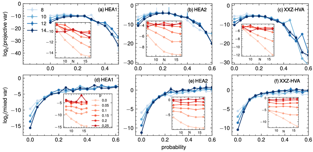
Figure 3: (top) Logarithmic variance of projective gradients as a function of probability of placing a measurement gate for (a) HEA1, (b) HEA2, and c) XXZ-HVA ansatz for system sizes $N=8-16$ and depth $16$. Inset shows that the projective variance becomes less severe with higher probability of measurement for $p=0-0.3$. Nevertheless, after a certain value, the projective gradient decays exponentially with the probability.(bottom)Logarithmic variance of the mixed gradients as a function of probability of placing a measurement gate for (c) HEA1, (d) HEA2, and (e) XXZ-HVA ansatz for system sizes $N=8-16$. The variance grows rapidly with the probability and settles to a constant value around $p=0.2$. Insets show the variance as a function of number of qubits. It can be concluded from the insets that the barren plateau become less severe with the more measurement gates and completely disappears around $p=0.15$ for all ansatzes.

We have computed variances of cost function gradients, a key indicator of BPs[12], systems sizes up to 18 qubits and circuit depts up to 100 layers of each ansatz presented in Fig. 2. Before presenting the results, we define the cost functions we use carefully.

The intermediate measurements in hybrid variational quantum circuits yield different outcomes for each run. We can compute the expectation value of observables either by (i) post-selecting for a specific outcome set $\mathbf{M}$ or (ii) averaging over all the measurement outcomes. Post-selection requires exponentially many samples in the number of measurement gates. However, if the expectation value is averaged over all the measurement outcomes, it corresponds to computing the expectation value with respect to the average density matrix. Thus, we define two types of cost functions, an projective cost functions computed with post-selected measurement outcomes and an mixed cost function computed ignoring measurement outcomes.

The projective cost function refers to the expectation value of an observable $\hat{O}$ calculated for a post-selected wave function. Consider, for example, a circuit consisting of a layer of unitary $\hat{U}({\bm{\theta}})$ and a projective measurement. A variational circuit will have many such unitary and measurement layers, but the same results can be used for the deeper circuit a we will show in Appendix  3.3. We define the projective cost function, post-selected for outcome $\mathbf{M}$ as follows:

$$C_{\textbf{M}}({\bm{\theta}})=\expectationvalue{\hat{O}}{\psi_{\mathbf{M}}({\bm{\theta}})}=\Tr[\hat{O}\hat{\rho}_{\mathbf{M}}],$$ (2)

where $\rho_{\mathbf{M}}({\bm{\theta}})=\ket{\psi_{\mathbf{M}}({\bm{\theta}})}\bra{\psi_{\mathbf{M}}({\bm{\theta}})}$ is the state projected onto measurement outcome $\mathbf{M}$ with projection operator $\hat{P}_{\mathbf{M}}$, and probability $p_{\mathbf{M}}$ as given below:

$$\ket{\psi_{\mathbf{M}}({\bm{\theta}})} =\frac{\ket{\tilde{\psi}_{\mathbf{M}}({\bm{\theta}})}}{\sqrt{p_{\mathbf{M}}({\bm{\theta}})}}=\frac{\hat{P}_{\mathbf{M}}\hat{U}({\bm{\theta}})\ket{0}}{\sqrt{\bra{0}\hat{U}^{\dagger}({\bm{\theta}})\hat{P}_{\mathbf{M}}\hat{U}({\bm{\theta}})\ket{0}}}.$$ (3)

Likewise, the mixed cost function is obtained by averaging the expectation value of an observable $\hat{O}$ over all possible measurement outcomes i.e.,

$$C({\bm{\theta}})=\mathbb{E}[C_{\mathbf{M}}({\bm{\theta}})] =\sum_{\mathbf{M}}p_{\mathbf{M}}({\bm{\theta}})\expectationvalue{\hat{O}}{\psi_{\mathbf{M}}({\bm{\theta}})}$$ (4)

$$=\Tr[\hat{O}\hat{\rho}({\bm{\theta}})].$$ (5)

In other words, mixed cost function is the expectation value with respect to the measurement-averaged density matrix $\hat{\rho}=\sum_{\mathbf{M}}p_{\mathbf{M}}\hat{\rho}_{\mathbf{M}}$.

The post-selected (projective) wavefunctions are free from barren plateaus at some carefully chosen probability range of placing a measurement gate. Fig. 3 clearly shows barren plateaus at $p=0$. Nevertheless, as we increase the probability of measuring, the barren plateau seems to get less severe, i.e., the gradient goes from exponential scaling with system sizes to some constant over a probability range (somewhere around $p=0.2$), then decays exponentially with probability until it hits the machine’s precision. This exponential decay differs from barren plateaus because the exponential decay of gradients with the system size characterizes barren plateaus. Note that projective gradients in Fig 3 are averaged over various measurement outcomes, so the error bars are higher for more measurement gates as the number of possible outcomes scales like $2^{M}$, where $M$ is the number of measurement gates. We refer to this region of exponentially small gradients as the “quantum Zeno” phase, a term coined by Li et al. [2] for quantum states that are frequently measured, and hence stalled close to an eigenstate of the measurement operator. Moreover, we are post-selecting for outcomes $\mathbf{M}$; consider $\mathbf{M}=\{0,0\cdots,0\}$ and $p=1.0$, then the expectation value of an operator $\hat{O}$ is always going to be $\expectationvalue{\hat{O}}{00\cdots 00}$ with no dependence on the variational parameters. The measurements essentially cut the communication between the parameters at the beginning of the circuit and the end, hence diminishing gradients.

The value of probability at which the barren plateau disappears depends on two factors: (i) the depth of the circuit and (ii) ansatz. The effect of depth on the projective gradients is to shift the turning point towards $p=0$, eventually stopping at $p\approx 0.2$. The dependence on the ansatz is much weaker than the dependence on the circuit depth. As a result, we don’t find the landscape transition coinciding with the measurement-induced phase transition in our projective gradients as reported by Wiersema et al. [1]. To understand this observation, we recall that MIPT cannot be observed in linear observables; hence, the gradients $\partial_{\theta}\expectationvalue{\hat{U}_{1}^{\dagger}(\theta)\hat{U}_{2}^{\dagger}H\hat{U}_{2}\hat{U}_{1}(\theta)}=i\langle 0|\hat{U}_{1}^{\dagger}[\hat{P},\hat{U}^{\dagger}_{2}\hat{H}\hat{U}_{2}]\hat{U}_{1}|0\rangle$ for $\hat{U}_{1}=e^{-i\theta\hat{P}}$ cannot detect the measurement-induced criticality. Based on the numerical evidence, we construct a potential phase diagram shown in Fig. 7.

mixed gradients: The mixed gradients always seem to have the same basic structure i.e., the gradient grows with the probability of measurement and plateaus to a constant value after around $p=0.2$. Exponential vanishing of gradients i.e, BP in this case is compensated for by summing over exponentially many measurements. Unlike the projective gradient, the location of the turning point is independent of the depth of the ansatz. Here, we still destroy the barren plateau at the same critical value as in the case of projective gradients but this doesn’t seem useful for optimization.

2.2 Landscape visualization of the optimization process

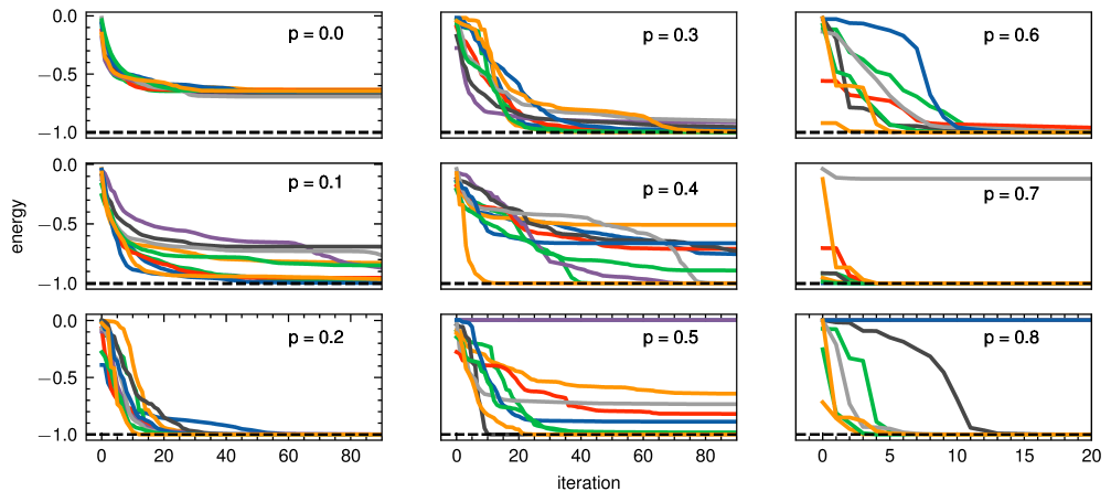
Figure 4: Mitigating barren plateaus with measurements and post-selection for a 8-qubit system with cost function $\hat{Z}_{0}\hat{Z}_{1}$. Each sub-figure corresponding to a measurement probability between 0 and 0.8 contains traces from 10 individual optimization runs carried out for the HEA2 ansatz with depth 20. Dashed line shows the exact ground state energy.

In the previous section, we focused on the optimization problem at the beginning of the optimization algorithm. We did so by examining the variance of the gradients of different cost functions computed on randomly generated initial states. This analysis can explain the difficulty of optimizing a circuit at the beginning of the optimization loop, but it does not directly address what happens at later optimization stages. Here we present optimization traces that show the path the algorithm takes through the cost landscape and seek to determine if measurements significantly alter these paths and whether a landscape transition is good for optimization in practice. We end with a visualization of the cost landscape near a local minimum using a technique common in machine learning literature for visualizing loss landscapes of neural networks[37].

In short, we find that the optimization traces benefit from the improved variance of hybrid variational ansatzes, thus mitigating the BP problem. The optimization runs were carried out for the projective cost function corresponding to the HEA2 ansatz for $\hat{Z}_{0}\hat{Z}_{1}$ and $XXZ$ Hamiltonians. For the $\hat{Z}_{0}\hat{Z}_{1}$ Hamiltonian, the cost function depends only on the first two qubits, and the initial computational basis state satisfies the minimum value. Nevertheless, optimizing a circuit with a depth of 20 to get this simple product state is challenging because of the BP, as shown in Fig. 4. Inserting measurement gates results in the optimization traces exploring various energies, with some reaching the minima. For higher probabilities, the optimization traces again get stuck at some parameter values. However, most happen to satisfy the minimum value because of the simple nature of the cost function with enormously degenerate global minima.

In appendix B, we present optimization traces on the $XXZ$ Hamiltonian ground state problem, which show similar but more complex behavior. In general we find measurements seem to help for some ansatzes more than others. For the HEA2 ansatz, they seem to work well, but for HEA2 with flexible parameters (not shown), and the XXZ the results are more mixed.

Although the variance of the mixed gradient increases with an increase in the number of measurement gates, they optimize poorly. The optimization trace (not shown here) gets noisier with the probability of placing a measurement. This suggests a noisy cost landscape for the mixed cost function.

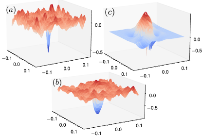
Figure 5: Cost landscape visualizations of the monitored HEA2 hybrid variational circuits with $\hat{O}=Z_{0}Z_{1}$. Visualizations are produced by optimizing the circuit and then plotting $C({\bm{\theta}})$ along two random directions in ${\bm{\theta}}$-space, where the origin is the minima achieved (a) no measurements showing a large barren plateau with a narrow path to the optimal state, (b) measurement probability $p=0.1$ showing a small barren plateau with a broad path to the optimal state, and (c) $p=0.8$ showing the quantum Zeno region, where the landscape is smooth and flat with broad suboptimal minima and a large volcano-like entrance to the optimal state.

Since the optimization traces are complex, we turned to visualizing the cost landscape near a local minimum. Following Ref. [37], we can visualize the cost landscape by randomly choosing two directions in Alice’s parameter space and plotting the cost function on the plane spanned by these essentially orthogonal directions. The results for the HEA2 cost function are presented in Fig. 5. In the absence of measurements, they show a rough BP with a very sharp drop to the local minima. This sharp drop broadens in the presence of measurements while the BP nevertheless persists. Then at a large measurement rate, in the quantum Zeno phase, the BP is absent, the landscape is smooth, and a volcano-like entrance guards the path to the minimum, explaining the difficulty of finding this minimum and getting out of it once one is inside.

2.3 Entanglement vs Landscape phase transitions

In section 1.1, we argued on information theoretic grounds that the MILT is different from the MIPT. Here we provide evidence that the MILT is a phase transition in an information-theoretic property of optimization problems before turning to a careful analysis of the MIPT in the three ansatzes we have been examining in this manuscript.

We can compute the mutual information $I(A,B)$ between Alice’s classical information and Bob’s measurement results following the discussion in the methods section, Sec. 3.2. Focusing on the HEA2 ansatz, one option for Bob’s measurements is to allow Bob to use the full computational basis, which is an eigenbasis of $\hat{O}=\hat{Z}_{0}\hat{Z}_{1}$. Here we choose to use the simpler option of allowing Bob just to measure $\hat{Z}_{0}\hat{Z}_{1}$ directly. We further simplify by allowing no mid-circuit measurements. Thus, this classical communication channel, which is the classical-quantum channel followed by Bob’s measurements, is given by the conditional probability $p(i\mid\theta)$ with Bob’s two measurement outcomes $i=-1,1$ and Alice’s parameters $\theta$ chosen uniformly across the entire parameter space. In this way, we have computed $I(A,B)$.

The results are presented in Fig. 6. They show $I(A,B)$, for circuits with depth $L\gtrsim N$, experiences an exponential drop in system size. Indeed $I(A,B)$ behaves very similarly to the variance of the gradients. Further, Fig. 6 appears nearly identical to the original results that help establish the existence of BPs[12] up to a factor of 10 in the layer depth. Specifically, $I(A,B)$ saturates above a circuit depth of approximately $1/10$ that of the saturation of the variance of the gradients. Hence, the mutual information captures the BP similarly to the variance of the gradients.

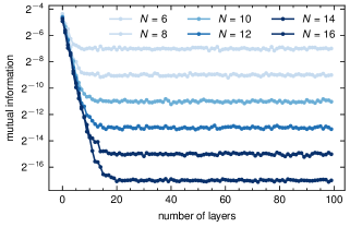
Figure 6: Mutual information $I(A,B)$ between Alice and Bob in the HEA2 ansatz with zero measurements, Bob measuring $\hat{O}=\hat{Z}_{0}\hat{Z}_{1}$, and Alice drawing parameters ${\bm{\theta}}$ uniformly. System sizes range between 6 and 16 qubits. The results show an exponential drop in $I(A,B)$ with system size.

Let us now turn to identifying the MIPT in our three ansatzes. To do so, we rely on computing the subsystem von-Neumann entropy to identify the entanglement phase transition. We note that two of them have been studied previously by Wiersema et. al [1]. It is crucial that the entropy is calculated for the post-selected states and averaged over various circuit realizations and measurement outcomes rather than vice-versa. For a specific circuit realization, the von Neumann entropy of a subsystem A is given by

$$S(A)=\Tr[\hat{\rho}_{A}\log_{2}\hat{\rho}_{A}],$$ (6)

where $\hat{\rho}_{A}=\Tr_{\bar{A}}[\ket{\psi}\bra{\psi}]$.

When the measurement gates are placed with high probability ($p>p_{c}$), the resulting state lies close to a trivial product state in the Hilbert space, and the late-time entanglement exhibits area-law scaling with the subsystem size i.e. $S(A)\propto|\partial A|$. However, if the measurement gates are too sparse ($p<p_{c}$), the subsystem appears close to a thermal state, exhibiting volume-law scaling, i.e., $S(A)\propto|A|$. At $p=p_{c}$, the critical point, the subsystem entanglement violates the area law logarithmically, i.e., $S(A)\propto\ln|A|$.

The entanglement entropy calculation was carried out for system sizes $N=6-18$. Detecting the critical point, therefore, requires finite-size scaling analysis. Inspired by prior success [4, 3, 27, 38, 1, 23], we use the scaling ansatz of the following form

$$S(p,N)-S(p_{c},N)=F((p-p_{c})N^{1/\nu}),$$ (7)

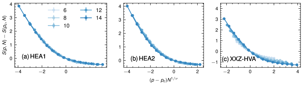
Figure 8: Finite-size scaling data collapse of the average entanglement entropy for (a) HEA1, (b)HEA2, and (c)XXZ-HVA ansatz used to extract the critical probabiltiy $p_{c}$, and scaling exponent $\nu$. XXZ-HVA lacks $N=18$ datapoints.

where $F(x)$ is the scaling function. In appendix 8, we plot the left-hand side as a function of $(p-p_{c})N^{1/\nu}$, and see a scaling collapse as shown in Fig. 8 also presented in the appendix. Importantly, these collapses occur with the exponent of $p-p_{c}$ set to 1. The critical parameters extracted from the numerics are listed in Table 1. We provide further details on numerics in Appendix 8. They show, as summarized in Fig. 7, the MIPT occurs at an ansatz-specific critical value of $p$, up to 2.5 times larger than the $p=0.2$ where, in the gradient analyses of Sec. 2.1, the BP universally collapses.

Ansatz	$p_{c}$	$\nu$
HEA1	$0.42\pm 0.02$	$1.18\pm 0.03$
HEA2	$0.48\pm 0.01$	$1.25\pm 0.04$
XXZ-HVA	$0.27\pm 0.02$	$1.26\pm 0.06$

Table 1: Critical measurement rate $p_{c}$ and correlation length exponent $\nu$ obtained numerically by finite size scaling of the von-Neumann entropy.

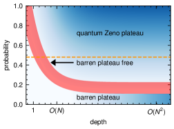
Figure 7: Phase diagram of variational quantum circuits showing the MILT region (shown in red) between barren plateau region and quantum Zeno region. The variance of the gradients is maximum in the crossover region and optimization the easiest. Orange dotted line shows the MIPT transition for HEA2 ansatz.

2.4 Discussion

The existence of the BP in the absence of measurements and in the presence of a low rate of measurements, both in the variance studies of Fig. 3, and the visualizations of Fig. 5 provide strong evidence the BP is a stable “phase” in optimization. Similarly, the quantum Zeno effect is observed at a high measurement rate if Bob is aware of the measurement outcomes. Like in the BP phase, Bob cannot decode much of Alice’s information. But here, the decoding problem is different. The projections produced by the measurements significantly weaken the dependence of the output state on Alice’s parameters. This weakening largely doesn’t depend on system size. It is a local effect. It is also characterized by a smoother cost landscape and, in some cases, by the volcano-like entrance to local minima, as presented in Fig. 5c. Since the scaling of the variance of gradients is different here, this “phase” must be separated from the BP phase by a phase transition.

In this study we have focused on the use of measurements to destroy a BP, but another simple approach is to study shorter circuits. The BP requires a significant entanglement growth and shorter circuits cut-off this growth. Hence, like we find landscape phase transitions as one tunes measurements, we predict such transitions will also occur as one tunes the circuit depth. Deep circuits will have a BP with gradients suppressed exponentially with system size while shallow circuits will have saturated gradients independent of system size. Given that a shallow circuit requires fewer resources, it would be interesting to determine which landscape transition are more helpful for optimization. In our preliminary attempts to study this question, we find the answer seems to be ansatz dependent, with some ansatzes benefiting more from measurements while others benefit more from shorter circuits.

Our results leave an important question unanswered. Coming down from a high measurement rate, at a critical value $p_{c}$, the quantum Zeno effect vanishes, and volume-law entanglement growth emerges via a MIPT. Rising up from $p=0$ the BP, as defined and observed by the variance of the gradients in 3, vanishes at $p=0.2$. Hence, between $p=0.2$ and $p_{c}$, there is no BP and no quantum Zeno effect. What then exists in this intermediate region, and what causes the collapse of the BP?

We can partly answer this question by recalling several observations. $\hat{O}$ is a linear quantum observable and is therefore insensitive to the MIPT. Further, the mixed gradients also observe the collapse of the BP at $p=0.2$, not just the post-selected projective gradients. So another agent than the quantum Zeno effect must be at play in this region and it causes the BP to collapse. A deeper quantum information theoretical study of this region may reveal what this agent is.

3 Methods

3.1 Numerical Simulations

We developed a Python statevector simulation library using Pytorch [39] to generate our numerical results which includes three kinds of ansatzes discussed in Sec. 1.2, namely (a) HEA1, (b) HEA2, and (c) XXZ-HVA. A unitary layer corresponding to a specific ansatz type is followed by a layer of projective measurements with probability $p$ per qubit. The measurements are implemented by the application of projection operators

For each measured qubit, we calculate the probability $p_{0}=|\langle 0|\psi({\bm{\theta}})\rangle|^{2}=\langle\psi({\bm{\theta}})|P_{0}|\psi({\bm{\theta}})\rangle$ and project onto $\ket{0}$ with probability $p_{0}$ or $\ket{1}$ with probability $1-p_{0}$. The results for variances and entanglement entropies presented in this paper are obtained by averaging over circuit realizations and measurement outcomes as follows:

$$\mathbb{E}\left[\expectationvalue*{\hat{O}}_{\mathbf{M}}\right]\approx\frac{1}{N_{s}}\sum_{\mathcal{C}}\expectationvalue*{\hat{O}}_{\mathbf{M}|\mathcal{C}},$$ (8)

where $N_{s}$ measurement outcome bitstrings ($\mathbf{M}$) corresponding to some circuit realization ($\mathcal{C}$) are sampled. Realizing a circuit $\mathcal{C}$ consists of randomly choosing parameters from $[-\pi,\pi]$ and location of the measurement gates. This portion of the computation involves sampling from a classical probability distribution whereas choosing the measurement outcomes $\mathbf{M}$ involves sampling from a quantum wavefunction. We used $N_{s}=10^{3}$ unless specified otherwise, and the error bars were determined using statistical bootstrapping method available in SciPy library [40, 41].

The numerical gradients presented in this work were calculated using analytical expressions. For example, gradient of the post-selected cost function i.e., the projective gradient can be analytically computed as follows:

$$\scalebox{0.91}{\mbox{$\displaystyle\partial_{k}C_{\mathbf{M}}({\bm{\theta}})=2\text{Re}\left[\frac{\bra*{\partial_{k}\tilde{\psi}_{\mathbf{M}}}\hat{O}\ket*{\tilde{\psi}_{\mathbf{M}}}}{p_{\mathbf{M}}}\right.\left.\frac{\expectationvalue*{\hat{\tilde{O}}}_{\mathbf{M}}}{p_{\mathbf{M}}^{2}}\bra*{\partial_{k}\tilde{\psi}_{\mathbf{M}}}\ket*{\tilde{\psi}_{\mathbf{M}}}\right]$}}.$$ (9)

A detailed derivation of this expression is given in Appendix  3.3. We show in Appendix 3.4 this gradient can also be computed using the parameter shift method[1, 42]:

$$\scalebox{0.85}{\mbox{$\displaystyle\partial_{k}C_{\mathbf{M}}({\bm{\theta}})=\frac{1}{2}\left(\expectationvalue*{\hat{O}_{\mathbf{M}}(\bm{\theta^{+}})}\frac{p_{\mathbf{M}}({\bm{\theta}}^{+})}{p_{\mathbf{M}}({\bm{\theta}})}-\expectationvalue*{\hat{O}_{\mathbf{M}}(\bm{\theta^{-}})}\frac{p_{\mathbf{M}}({\bm{\theta}}^{-})}{p_{\mathbf{M}}({\bm{\theta}})}\right)$}},$$ (10)

where we define the shifted parameters as $\mathbf{\theta^{+}}=\{\theta_{1},\cdots,\theta_{k}+\frac{\pi}{2},\cdots\}$ and $\mathbf{\theta^{-}}=\{\theta_{1},\cdots,\theta_{k}-\frac{\pi}{2},\cdots\}$.

Similarly, the mixed gradient can be expressed as

$$\partial_{k}C({\bm{\theta}}) =\sum_{\mathbf{M}}2\text{Re}\left[\bra*{\partial_{k}\tilde{\psi}_{\mathbf{M}}({\bm{\theta}})}O\ket*{\tilde{\psi}_{\mathbf{M}}({\bm{\theta}})}\right].$$ (11)

The mixed gradient can also be obtained by using the parameter shift method i.e.,

$$\partial_{k}C({\bm{\theta}})=\frac{1}{2}\left(C({\bm{\theta}}^{+})-C({\bm{\theta}}^{-})\right).$$ (12)

In addition to variance analysis, we performed optimization runs to minimize the energy of two cost functions: (i) $\hat{Z}_{0}\hat{Z}_{1}$, and (ii) the XXZ Hamiltonian given by:

$$H_{XXZ}=\sum_{i=0}^{L}\hat{X}_{i}\hat{X}_{i+1}+\hat{Y}_{i}\hat{Y}_{i+1}+\Delta\hat{Z}_{i}\hat{Z}_{i+1},$$ (13)

where $(L+1)^{th}$ qubit is identified with the $0^{th}$ qubit to impose periodic boundary. We used the L-BFGS-B algorithm [43] to optimize the HEA2 ansatz with 8 qubits, 16 layers and various measurement probabilities $p$. For each case, we generated 10 optimization traces starting from randomly generated initial parameters and circuit realizations.

Furthermore, we visualized the cost landscape around the optimal point. Some of the representative landscapes are shown in Fig. 5. After the convergence of our optimizer, we generated a 2d grid by taking two random vectors around the minima and evaluated the cost function at these points. We find that the cost landscape can be used as an effective tool to diagnose the trainability of an ansatz.

3.2 Estimating the mutual information of classical-quantum channels with measurements

Alice is going to choose a parameter value $\theta$ from a distribution $p_{A}(\theta)$, then send it to Bob via a classical-quantum channel $\theta\mapsto\rho_{\theta}$. Bob then carries out POVM measurements $E_{i}$ and obtains the probabilities of the measurement outcomes $p(i|\theta)=\Tr[\rho_{\theta}E_{i}]$. Bob then needs to determine $\theta$. This sets up a classical information channel between Alice and Bob. If, along the way, measurements happen and Bob is projective of these measurement outcomes, then Bob can use this additional information to determine $\theta$. The information channel is then $p(i,m|\theta)$. Below we compute the mutual information $I(A,B)$ between Alice and Bob. Optimizing $I(A,B)$ over Alice’s distribution $p(\theta)$ would give Shannon’s channel capacity, a task we have not studied in this manuscript.

Below we compute an efficient sample-averge estimator for the mutual information in different circumstances.

3.2.1 The noiseless channel

Here no measurements take place. Then $p(i|{\bm{\theta}})=\Tr[\rho_{\bm{\theta}}E_{i}]$ are the probabilities of Bob’s measurement outcomes. The mutual information is given by $I(A,B)=S_{A}+S_{B}-S_{A,B}$ where $S_{A}$ is the entropy of the distribution $p_{A}({\bm{\theta}})$, $S_{A,B}$ the entropy of the distribution $p(i|{\bm{\theta}})p_{A}({\bm{\theta}})$ and $S_{B}$ the entropy of the distribution $p_{B}(i)=\int d{\bm{\theta}}p(i|{\bm{\theta}})p_{A}({\bm{\theta}})$.

To compute $S_{A}$ and $S_{A,B}$, we must carefully treat these continuous probability distributions’ entropy. We do so by discretizing the parameter space ${\bm{\theta}}$ into $M$ parameter values $\{{\bm{\theta}}_{1},{\bm{\theta}}_{2},\ldots,{\bm{\theta}}_{M}\}$, each occupying a volume $\Delta{\bm{\theta}}$ such that $\lim_{M\to\infty}\sum_{i}\Delta{\bm{\theta}}p({\bm{\theta}}_{i})=\int d{\bm{\theta}}p({\bm{\theta}})=1$. If $V$ is the volume of the continuous space and $q({\bm{\theta}})$ the uniform distribution over it, then $\Delta{\bm{\theta}}=V/M$ and $q({\bm{\theta}})=1/V$. We these definitions, the entropy for finite $M$ is approximately

$$S(A)=\log M-\int d{\bm{\theta}}\,p_{A}({\bm{\theta}})\log\frac{p_{A}({\bm{\theta}})}{q({\bm{\theta}})}$$ (14)

Similarly, we also find

$$S_{A,B}=\log M-\sum_{i}\int d{\bm{\theta}}\,p(i\mid{\bm{\theta}})p_{A}({\bm{\theta}})\log\frac{p(i\mid{\bm{\theta}})p_{A}({\bm{\theta}})}{q({\bm{\theta}})}$$ (15)

so we can safely send $M\to\infty$ in the mutual information $I(A,B)=S_{A}+S_{B}-S_{A,B}$.

Bob’s entropy $S_{B}$, is computed from a discrete distribution. So we can use the standard Shannon entropy. Computing $p_{B}(i)$ we find

$$p_{B}(i) =\int d{\bm{\theta}}\,p(i\mid{\bm{\theta}})p_{A}({\bm{\theta}}),$$ (16)

Then, we can obtain $S_{B}=-\sum_{i}p_{B}(i)\log p_{B}(i)$.

Putting these results together to compute the mutual information, we find

$$I(A,B) =-\sum_{i}\int d{\bm{\theta}}\,p(i\mid{\bm{\theta}})p_{A}({\bm{\theta}})\log\frac{p_{B}(i)}{p(i\mid{\bm{\theta}})}$$ (18)

$$=-\sum_{a,b}\frac{1}{N_{a}N_{b}}\log\frac{p_{B}(i_{b|a})}{p(i_{b|a}\mid{\bm{\theta}}_{a})}$$ (19)

Where in the last line we sample $p(i\mid{\bm{\theta}})p_{A}({\bm{\theta}})$ by sampling $p_{A}({\bm{\theta}})$ to get ${\bm{\theta}}_{a}$, then sampling $p(i\mid{\bm{\theta}}_{a})$ to get $i_{b|a}$ and introduce the notation $a|b$ here to remind us that sample $i_{b}$ was obtained by first obtaining ${\bm{\theta}}_{a}$ then sampling $p(i\mid{\bm{\theta}}_{a})$. We also sent $M\to\infty$, so the result is exact.

3.2.2 Noisy channel, Bob is aware of measurements

Let us now consider the case where the channel suffers noise from an environment, but Bob is projective of the “measurements” that constitute this environment. Here the information channel is $p(i,m\mid{\bm{\theta}})=p(i|m,{\bm{\theta}})p(m\mid{\bm{\theta}})$ where $m$ denotes measurement outcomes. Given such a channel, we can again compute the mutual information as in the above noiseless case. So we can directly obtain $I(A,B)$ by sending $i\to i,m$. The result is

$$I(A,B) =-\sum_{i,m}\int d{\bm{\theta}}\,p(i,m\mid{\bm{\theta}})p_{A}({\bm{\theta}})\log\frac{p_{B}(i,m)}{p(i,m\mid{\bm{\theta}})}$$ (20)

$$=-\sum_{a,b,c}\frac{1}{N_{a}N_{b}N_{c}}\log\frac{p_{B}(i_{c|a,b},m_{b|a})}{p(i_{c|a,b},m_{b|a}\mid{\bm{\theta}}_{a})}$$ (21)

where the last line is the sample estimator for $I(A,B)$ given ${\bm{\theta}}_{a}$ drawn from $p_{A}({\bm{\theta}})$, $m_{b|a}$ drawn from $p(m\mid{\bm{\theta}}_{a})$ and $i_{c|a,b}$ drawn from $p(i\mid m_{b|a},{\bm{\theta}}_{a})$.

3.2.3 Noisy channel, Bob is unaware of measurements

Here we marginalize over the environment’s measurement outcomes. The channel is then given by $p(i\mid{\bm{\theta}})=\sum_{m}p(i,m\mid{\bm{\theta}})$. Hence, we can directly insert this into the mutual information of the noiseless case to obtain

$$I(A,B) =-\sum_{i}\int d{\bm{\theta}}\,p(i\mid{\bm{\theta}})p_{A}({\bm{\theta}})\log\frac{p_{B}(i)}{p(i\mid{\bm{\theta}})}$$ (22)

$$=-\sum_{a,b}\frac{1}{N_{a}N_{b}}\log\frac{p_{B}(i_{b|a})}{p(i_{b|a}\mid{\bm{\theta}}_{a})}$$ (23)

but now we need to estimate $p_{B}(i_{b|a})$ and $p(i_{b|a}\mid{\bm{\theta}}_{a})$. These are

$$p(i_{b|a}\mid{\bm{\theta}}_{a}) =\sum_{m}p(i_{b|a}\mid m,{\bm{\theta}}_{a})p(m\mid{\bm{\theta}}_{a})$$ (24)

$$=\sum_{c}\frac{1}{N_{c}}p(i_{b|a}\mid m_{c|a,b},{\bm{\theta}}_{a})$$ (25)

$$p_{B}(i_{b|a}) =\int d{\bm{\theta}}\,p(i_{b|a}\mid{\bm{\theta}})p_{A}({\bm{\theta}})$$ (26)

$$=\sum_{c}\frac{1}{N_{c}}p(i_{b|a}\mid{\bm{\theta}}_{c})$$ (27)

3.3 Calculating projective and mixed gradients of monitored quantum circuits

The first layer of unitary $\hat{U}_{1}(\theta_{1})$ is applied to a quantum circuit initialized in the computational basis. The state of the circuit after projective measurement onto state $1$ is given by

$$\ket{\psi_{1}}=\frac{\hat{P}_{1}\hat{U}_{1}(\theta_{1})\ket{0}}{\sqrt{p_{1}}},\quad p_{1}=\bra{0}\hat{U}_{1}^{\dagger}(\theta_{1})\hat{P}_{1}\hat{U}_{1}(\theta_{1})\ket{0}.$$ (28)

After the second layer of unitary and projective measurement onto state $\mathbf{2}$,

$$\ket{\psi_{\mathbf{2}}} =\frac{\hat{P}_{2}\hat{U}_{2}(\theta_{2})\hat{P}_{1}\hat{U}_{1}(\theta_{1})\ket{0}}{\sqrt{p_{\mathbf{2}}}}$$ (29)

$$\quad p_{\mathbf{2}} =\bra{0}\hat{U}_{1}^{\dagger}(\theta_{1})\hat{P}_{1}\hat{U}_{2}^{\dagger}(\theta_{2})\hat{P}_{2}\hat{U}_{2}(\theta_{2})\hat{P}_{1}\hat{U}_{1}(\theta_{1})\ket{0},$$ (30)

where $\mathbf{2}=(1,2)$ Notice that $p_{1}$ in the denominator has cancelled out. By continuing this process for $M$ layers, we get

$$\ket{\psi_{\mathbf{M}}} =\frac{\hat{P}_{M}\hat{U}_{M}(\theta_{M})\cdots\hat{P}_{1}\hat{U}_{1}(\theta_{1})\ket{0}}{\sqrt{p_{\mathbf{M}}}}=\frac{\ket*{\tilde{\psi}_{\mathbf{M}}}}{\sqrt{p_{\mathbf{M}}}},$$ (31)

$$\quad p_{\mathbf{M}} =\bra*{\tilde{\psi}_{\mathbf{M}}}\ket*{\tilde{\psi}_{\mathbf{M}}},$$ (32)

where we have taken $\ket*{\tilde{\psi}_{\mathbf{M}}}=\hat{P}_{M}\hat{U}_{M}(\theta_{M})\cdots\hat{P}_{1}\hat{U}_{1}(\theta_{1})\ket{0}$, the unnormalized measured state. For a specific set of measurement outcomes $\mathbf{M}=(1,2,\cdots,M)$, the expectation value of an operator $\hat{O}$ is given by:

$$\expectationvalue*{\hat{O}}_{\mathbf{M}}=\bra{\psi_{\mathbf{M}}}\hat{O}\ket{\psi_{\mathbf{M}}}=\frac{\bra*{\tilde{\psi}_{\mathbf{M}}}\hat{O}\ket*{\tilde{\psi}_{\mathbf{M}}}}{p_{\mathbf{M}}}=\frac{\expectationvalue*{\hat{\tilde{O}}}_{\mathbf{M}}}{p_{\mathbf{M}}}$$ (33)

The ensemble average over all possible measurement outcomes is then

$$\mathbb{E}\left[\expectationvalue*{\hat{O}_{\mathbf{M}}}\right]=\sum_{\mathbf{M}}{p_{\mathbf{M}}}\expectationvalue*{\hat{O}}_{\mathbf{M}}$$ (34)

We also would like to do the same for gradients:

$$\partial_{k}\expectationvalue*{\hat{O}}_{\mathbf{M}}=\partialderivative{\expectationvalue*{\hat{O}}_{\mathbf{M}}}{\theta_{k}}=\frac{1}{p_{\mathbf{M}}}\partialderivative{\expectationvalue*{\hat{\tilde{O}}}_{\mathbf{M}}}{\theta_{k}}-\frac{\expectationvalue*{\hat{\tilde{O}}}_{\mathbf{M}}}{p_{\mathbf{M}}^{2}}\partialderivative{p_{\mathbf{M}}}{\theta_{k}}$$ (35)

We note that

$$\partialderivative{\expectationvalue*{\hat{\tilde{O}}}_{\mathbf{M}}}{\theta_{k}}=\matrixelement{\partial_{k}\tilde{\psi}_{\mathbf{M}}}{\hat{O}}{\tilde{\psi}_{\mathbf{M}}}+\matrixelement{\tilde{\psi}_{\mathbf{M}}}{\hat{O}}{\partial_{k}\tilde{\psi}_{\mathbf{M}}},$$ (36)

and

$$\partialderivative{p_{\mathbf{M}}}{\theta_{k}}=\bra*{\partial_{k}\tilde{\psi}_{\mathbf{M}}}\ket*{\tilde{\psi}_{\mathbf{M}}}+\bra*{\tilde{\psi}_{\mathbf{M}}}\ket*{\partial_{k}\tilde{\psi}_{\mathbf{M}}}$$ (37)

Putting them back to Eqn. 35, we get

$$\partial_{k}\expectationvalue*{\hat{O}}_{\mathbf{M}} =\frac{1}{p_{\mathbf{M}}}\bra*{\partial_{k}\tilde{\psi}_{\mathbf{M}}}\hat{O}\ket*{\tilde{\psi}_{\mathbf{M}}}-\frac{\expectationvalue*{\hat{\tilde{O}}}_{\mathbf{M}}}{p_{\mathbf{M}}^{2}}\bra*{\partial_{k}\tilde{\psi}_{\mathbf{M}}}\ket*{\tilde{\psi}_{\mathbf{M}}}+\>\text{c.c.}$$ (38)

Thus, the ensemble average of the gradients is:

$$\mathbb{E}\left[\partial_{k}\expectationvalue*{\hat{O}}_{\mathbf{M}}\right]=\sum_{\mathbf{M}}p_{\mathbf{M}}\,\partial_{k}\expectationvalue{\hat{O}}_{\mathbf{M}}$$

$$=\sum_{\mathbf{M}}p_{\mathbf{M}}\,2\text{Re}\{\frac{\bra*{\partial_{k}\tilde{\psi}_{\mathbf{M}}}\hat{O}\ket*{\tilde{\psi}_{\mathbf{M}}}}{p_{\mathbf{M}}}-\frac{\expectationvalue*{\hat{\tilde{O}}}_{\mathbf{M}}}{p_{\mathbf{M}}^{2}}\bra*{\partial_{k}\tilde{\psi}_{\mathbf{M}}}\ket*{\tilde{\psi}_{\mathbf{M}}}\}$$ (39)

By using equations (A4) and (A6), it is possible to get this into the form presented in equation (5). They are interchangeable in this way.

To acquire the gradient of the average, we start with:

$$\partial_{k}C({\bm{\theta}}) =\partial_{k}\sum_{\mathbf{M}}p_{\mathbf{M}}({\bm{\theta}})\langle\psi_{\mathbf{M}}({\bm{\theta}})|\hat{O}|\psi_{\mathbf{M}}({\bm{\theta}})\rangle$$ (40)

Putting in (A6), we can cancel out the factor of ${p_{\mathbf{M}}}$, and use equations (A4), (A9) to arrive at the desired identity.

$$\partial_{k}C({\bm{\theta}}) =\sum_{\mathbf{M}}\partial_{k}\langle\hat{\tilde{O}}\rangle_{\mathbf{M}}$$

$$=\sum_{\mathbf{M}}\partialderivative{\langle\hat{\tilde{O}}\rangle}{\theta_{k}}$$

$$=\sum_{\mathbf{M}}\matrixelement{\partial_{k}\tilde{\psi}_{\mathbf{M}}}{\hat{O}}{\tilde{\psi}_{\mathbf{M}}}+\matrixelement{\tilde{\psi}_{\mathbf{M}}}{\hat{O}}{\partial_{k}\tilde{\psi}_{\mathbf{M}}}$$

$$=\sum_{\mathbf{M}}2p_{\mathbf{M}}\text{Re}\{\matrixelement{\partial_{k}\psi_{\mathbf{M}}}{\hat{O}}{\psi_{\mathbf{M}}}\}$$ (41)

In practice, to calculate either gradient, we use ensemble averages. We calculate the ensemble average for an operator $\hat{O}$ by averaging over $N_{s}$ samples $\{\mathbf{M^{\prime}}\}$ drawn from $p_{\mathbf{M}}$. i.e.

$$\mathbb{E}\left[O_{\mathbf{M}}\right] =\sum_{\mathbf{M}}p_{\mathbf{M}}O_{\mathbf{M}}$$

$$=\frac{1}{N_{s}}\sum_{\mathbf{M^{\prime}}}O_{\mathbf{M^{\prime}}}.$$ (42)

3.4 Gradients using parameter shift

Let’s take a closer look at Eqn. 36 :

$$\partialderivative{\expectationvalue*{\hat{\tilde{O}}}_{\mathbf{M}}}{\theta_{k}}=\matrixelement{\partial_{k}\tilde{\psi}_{\mathbf{M}}}{\hat{O}}{\tilde{\psi}_{\mathbf{M}}}+\matrixelement{\tilde{\psi}_{\mathbf{M}}}{\hat{O}}{\partial_{k}\tilde{\psi}_{\mathbf{M}}}.$$ (43)

Noting that

$$\ket{\tilde{\psi}_{\mathbf{M}}}=\left(\prod_{i=k+1}^{M}\hat{P}_{i}\hat{U}_{i}(\theta_{i})\right)\hat{P}_{l}\hat{U}_{l}(\theta_{l})\left(\prod_{i=1}^{k-1}\hat{P}_{i}\hat{U}_{i}(\theta_{i})\right)\ket{0}$$ (44)

and

$$\ket{\partial_{k}\tilde{\psi}_{\mathbf{M}}}=-\frac{i}{2}\left(\prod_{i=k+1}^{M}\hat{P}_{i}\hat{U}_{i}(\theta_{i})\right)\hat{P}_{l}\hat{A}_{l}\hat{U}_{l}(\theta_{l})\left(\prod_{i=1}^{k-1}\hat{P}_{i}\hat{U}_{i}(\theta_{i})\right)\ket{0},$$ (45)

where $\hat{U}_{l}(\theta_{l})=\exp(-\frac{i}{2}\theta_{l}\hat{A}_{l})$. Suppose $\hat{O}^{\prime}=\hat{P}_{l}^{\dagger}\left(\prod_{i=M}^{k+1}\hat{U}_{i}^{\dagger}\hat{P}^{\dagger}_{i}(\theta_{i})\right)\hat{O}\left(\prod_{i=k+1}^{M}\hat{P}_{i}\hat{U}_{i}(\theta_{i})\right)\hat{P}_{l}$, and $\ket{\psi^{\prime}}=\hat{U}_{l}(\theta_{l})\left(\prod_{i=1}^{k-1}\hat{P}_{i}\hat{U}_{i}(\theta_{i})\right)\ket{0}$. Then,

$$\partialderivative{\expectationvalue*{\hat{\tilde{O}}}_{\mathbf{M}}}{\theta_{k}} =\frac{i}{2}\left(\bra{\psi^{\prime}}\hat{A}_{l}\hat{O}^{\prime}\ket{\psi^{\prime}}-\bra{\psi^{\prime}}\hat{O}^{\prime}\hat{A}_{l}\ket{\psi^{\prime}}\right)$$ (46)

$$=\frac{i}{2}\bra{\psi^{\prime}}\left[\hat{A}_{l},\hat{O}^{\prime}\right]\ket{\psi^{\prime}}$$ (47)

The parameter-shift rule states:

$$\left[\hat{A}_{l},\hat{O}^{\prime}\right]=-i\left(\hat{U}_{i}^{\dagger}\left(\frac{\pi}{2}\right)\hat{O}^{\prime}\hat{U}_{i}\left(\frac{\pi}{2}\right)-\hat{U}_{i}^{\dagger}\left(-\frac{\pi}{2}\right)\hat{O}^{\prime}\hat{U}_{i}\left(-\frac{\pi}{2}\right)\right)$$ (48)

Substituting this back,

$$\partialderivative{\expectationvalue*{\hat{\tilde{O}}}_{\mathbf{M}}}{\theta_{k}} =\frac{1}{2}\left(\matrixelement{\partial_{k}\tilde{\psi}_{\mathbf{M}}}{\hat{O}}{\tilde{\psi}_{\mathbf{M}}}^{+}-\matrixelement{\partial_{k}\tilde{\psi}_{\mathbf{M}}}{\hat{O}}{\tilde{\psi}_{\mathbf{M}}}^{-}\right)$$ (49)

$$=\frac{1}{2}\left(\frac{\matrixelement{\partial_{k}\tilde{\psi}_{\mathbf{M}}}{\hat{O}}{\tilde{\psi}_{\mathbf{M}}}^{+}}{p_{\mathbf{M}}^{+}}p_{\mathbf{M}}^{+}-\frac{\matrixelement{\partial_{k}\tilde{\psi}_{\mathbf{M}}}{\hat{O}}{\tilde{\psi}_{\mathbf{M}}}^{-}}{p_{\mathbf{M}}^{-}}p_{\mathbf{M}}^{-}\right)$$

$$=\frac{1}{2}\left(\expectationvalue*{\hat{O}}^{+}p_{\mathbf{M}}^{+}-\expectationvalue*{\hat{O}}^{-}p_{\mathbf{M}}^{-}\right),$$ (50)

where $(.)^{\pm}$ denotes the expectation value calculated at parameter values $(\theta_{1},\cdots,\theta_{l}\pm\frac{\pi}{2},\cdots,\theta_{M})$. Similarly, taking a closer look at Eq. 37:

$$\partialderivative{p_{\mathbf{M}}}{\theta_{k}} =\bra*{\partial_{k}\tilde{\psi}_{\mathbf{M}}}\ket*{\tilde{\psi}_{\mathbf{M}}}+\bra*{\tilde{\psi}_{\mathbf{M}}}\ket*{\partial_{k}\tilde{\psi}_{\mathbf{M}}}$$ (51)

$$=\frac{1}{2}\left(p_{\mathbf{M}}^{+}-p_{\mathbf{M}}^{-}\right)$$ (52)

Now, writing Eq. (35) in terms of parameter-shifted quantities,

$$\partial_{k}\expectationvalue*{\hat{O}}_{\mathbf{M}}=\partialderivative{\expectationvalue*{\hat{O}}_{\mathbf{M}}}{\theta_{k}}=\frac{1}{p_{\mathbf{M}}}\partialderivative{\expectationvalue*{\hat{\tilde{O}}}_{\mathbf{M}}}{\theta_{k}}-\frac{\expectationvalue*{\hat{\tilde{O}}}_{\mathbf{M}}}{p_{\mathbf{M}}^{2}}\partialderivative{p_{\mathbf{M}}}{\theta_{k}}$$ (53)

$$=\frac{1}{2}\left(\expectationvalue*{\hat{O}}^{+}\frac{p_{\mathbf{M}}^{+}}{p_{\mathbf{M}}}-\expectationvalue{\hat{O}}^{-}\frac{p_{\mathbf{M}}^{-}}{p_{\mathbf{M}}}\right)-\frac{1}{2}\frac{\expectationvalue*{\hat{O}}}{p_{\mathbf{M}}}\left(p_{\mathbf{M}}^{+}-p_{\mathbf{M}}^{-}\right)$$ (54)

Acknowledgments We thank Yong-Baek Kim, Roeland Wiersema, and Juan Felipe Carrasquilla for useful discusions. This work was supported in part by the National Science Foundation grant number …

Appendix A Finite-size scaling analysis of measurement induced criticality

.

Although phase transitions are defined in the thermodynamic limit, we can use finite-size scaling analysis to study them numerically. With our exact state vector calculations, we were able to simulate systems only up to 18 qubits with $10^{3}$ samples for $N\leq 16$ and $500$ samples for $N=18$. We used the quality of the data collapse to determine the critical probability $p_{c}$, and critical exponent $\nu$.

The model for the finite-size scaling collapse is given in Eqn. 7. If there is a continuous phase transition at $p=p_{c}$, then the left hand side of this equation, computed close to $p_{c}$ should collapse into the scaling function of the parameter $(p-p_{c})L^{1/\nu}$. The fitting parameters are determined by the method described in Ref. [4]. We discuss this briefly for completeness.

We define a cost function $R(p_{c},\nu)$ for given values of critical parameters $p_{c}$ and $\nu$ which will be minimized to get the best estimates. $S(p_{c},N)$ for each system size $N$ is determined by linear interpolation and $x=(p-p_{c})N^{1/\nu}$, $y_{N}=S(p,N)-S(p_{c},N)$ are calculated for each data point. A family of curves $y_{L}(x)$ is obtained and the average of these curves calculated to get the mean $\bar{y}(x)$, to which all our data points will hopefully collapse. The cost function is defined as

$$R=\sum_{i,L}\left[y_{L}(x_{i})-\bar{y}(x_{i})\right]^{2}.$$ (55)

The fitting cost function was minimized using L-BFGS-B routine available in Scipy library to get an estimate for $p_{c}$ and $\nu$. Once a good estimate was found, random initial values in their neighborhood were used as initial parameters and $5$ different estimates were collected. The values reported in Table 1 are the means of those estimates and the error bars are the standard deviations. Better estimates for $N\rightarrow\infty$ can be found by iterating through the process of limiting the dataset to some $N$ and doing a fit for $p_{c}$ and $\nu$ vs $1/N$ and taking the y-intercept. We did not go through this exercise since the measurement induced entanglement phase transition is not the main topic of our study.

Appendix B Optimization traces for XXZ cost function

We here examine the optimization traces for a $XXZ$ Hamiltonian with the same variational circuits. Similar to the $\hat{Z}_{0}\hat{Z}_{1}$ case of 4, we find that lower energy can be reached with a high likelihood with hybrid variational ansatzes compared to the unitary ansatzes. Before getting stuck in a quantum Zeno state, the circuits with a low probability of measurement ($p<0.2$) explore a broader range of energy as indicated by our variance results. However, the global minimum is never reached in this case because we chose the gapless region($\Delta<1$) of the phase diagram for optimization. Preparing a gapless ground state with either adiabatic evolution or VQE is a considerably tricky problem compared to a gapped one.

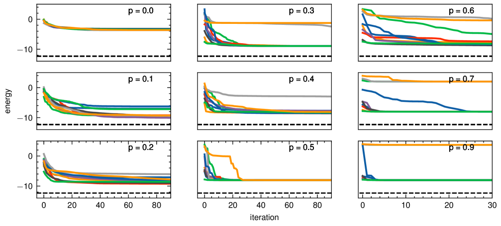
Figure 9: Mitigating barren plateaus with measurements and post-selection for a 8-qubit XXZ Hamiltonian with anisotropy parameter $\Delta=0.5$ Each sub figure, corresponding to a measurement probability between 0 and 0.8, contains traces from 10 individual optimization runs carried out for the HEA2 ansatz with depth 20. Dashed line shows the exact ground state energy.

References

- \bibcommenthead
- Wiersema et al. [2023] Wiersema, R., Zhou, C., Carrasquilla, J.F., Kim, Y.B.: Measurement-induced entanglement phase transitions in variational quantum circuits. SciPost Phys. 14, 147 (2023) https://doi.org/10.21468/SciPostPhys.14.6.147
- Li et al. [2018] Li, Y., Chen, X., Fisher, M.P.A.: Quantum zeno effect and the many-body entanglement transition. Phys. Rev. B 98, 205136 (2018) https://doi.org/10.1103/PhysRevB.98.205136
- Li et al. [2019] Li, Y., Chen, X., Fisher, M.P.A.: Measurement-driven entanglement transition in hybrid quantum circuits. Phys. Rev. B 100, 134306 (2019) https://doi.org/10.1103/PhysRevB.100.134306
- Skinner et al. [2019] Skinner, B., Ruhman, J., Nahum, A.: Measurement-induced phase transitions in the dynamics of entanglement. Phys. Rev. X 9, 031009 (2019) https://doi.org/10.1103/PhysRevX.9.031009
- Preskill [2018] Preskill, J.: Quantum Computing in the NISQ era and beyond. Quantum 2, 79 (2018) https://doi.org/10.22331/q-2018-08-06-79
- Peruzzo et al. [2014] Peruzzo, A., McClean, J., Shadbolt, P., Yung, M.-H., Zhou, X.-Q., Love, P.J., Aspuru-Guzik, A., O’Brien, J.L.: A variational eigenvalue solver on a photonic quantum processor. Nature Communications 5(1), 4213 (2014) https://doi.org/10.1038/ncomms5213
- McClean et al. [2016] McClean, J.R., Romero, J., Babbush, R., Aspuru-Guzik, A.: The theory of variational hybrid quantum-classical algorithms. New Journal of Physics 18(2), 023023 (2016) https://doi.org/10.1088/1367-2630/18/2/023023
- Cerezo et al. [2021] Cerezo, M., Arrasmith, A., Babbush, R., Benjamin, S.C., Endo, S., Fujii, K., McClean, J.R., Mitarai, K., Yuan, X., Cincio, L., Coles, P.J.: Variational quantum algorithms. Nature Reviews Physics 3(9), 625–644 (2021) https://doi.org/10.1038/s42254-021-00348-9
- Sim et al. [2019] Sim, S., Johnson, P.D., Aspuru-Guzik, A.: Expressibility and entangling capability of parameterized quantum circuits for hybrid quantum-classical algorithms. Advanced Quantum Technologies 2(12), 1900070 (2019) https://doi.org/10.1002/qute.201900070
- Haug et al. [2021] Haug, T., Bharti, K., Kim, M.S.: Capacity and quantum geometry of parametrized quantum circuits. PRX Quantum 2, 040309 (2021) https://doi.org/10.1103/PRXQuantum.2.040309
- Holmes et al. [2022] Holmes, Z., Sharma, K., Cerezo, M., Coles, P.J.: Connecting ansatz expressibility to gradient magnitudes and barren plateaus. PRX Quantum 3, 010313 (2022) https://doi.org/10.1103/PRXQuantum.3.010313
- McClean et al. [2018] McClean, J.R., Boixo, S., Smelyanskiy, V.N., Babbush, R., Neven, H.: Barren plateaus in quantum neural network training landscapes. Nature Communications 9(1), 4812 (2018) https://doi.org/10.1038/s41467-018-07090-4
- Cerezo et al. [2021] Cerezo, M., Sone, A., Volkoff, T., Cincio, L., Coles, P.J.: Cost function dependent barren plateaus in shallow parametrized quantum circuits. Nature Communications 12(1), 1791 (2021) https://doi.org/10.1038/s41467-021-21728-w
- Wang et al. [2021] Wang, S., Fontana, E., Cerezo, M., Sharma, K., Sone, A., Cincio, L., Coles, P.J.: Noise-induced barren plateaus in variational quantum algorithms. Nature Communications 12(1), 6961 (2021) https://doi.org/10.1038/s41467-021-27045-6
- Ortiz Marrero et al. [2021] Ortiz Marrero, C., Kieferová, M., Wiebe, N.: Entanglement-induced barren plateaus. PRX Quantum 2, 040316 (2021) https://doi.org/10.1103/PRXQuantum.2.040316
- Mele et al. [2022] Mele, A.A., Mbeng, G.B., Santoro, G.E., Collura, M., Torta, P.: Avoiding barren plateaus via transferability of smooth solutions in a hamiltonian variational ansatz. Phys. Rev. A 106, 060401 (2022) https://doi.org/10.1103/PhysRevA.106.L060401
- Grimsley et al. [2023] Grimsley, H.R., Barron, G.S., Barnes, E., Economou, S.E., Mayhall, N.J.: Adaptive, problem-tailored variational quantum eigensolver mitigates rough parameter landscapes and barren plateaus. npj Quantum Information 9(1), 19 (2023)
- Friedrich and Maziero [2022] Friedrich, L., Maziero, J.: Avoiding barren plateaus with classical deep neural networks. Phys. Rev. A 106, 042433 (2022) https://doi.org/10.1103/PhysRevA.106.042433
- Grant et al. [2019] Grant, E., Wossnig, L., Ostaszewski, M., Benedetti, M.: An initialization strategy for addressing barren plateaus in parametrized quantum circuits. Quantum 3, 214 (2019) https://doi.org/10.22331/q-2019-12-09-214
- Patti et al. [2021] Patti, T.L., Najafi, K., Gao, X., Yelin, S.F.: Entanglement devised barren plateau mitigation. Phys. Rev. Res. 3, 033090 (2021) https://doi.org/10.1103/PhysRevResearch.3.033090
- Sack et al. [2022] Sack, S.H., Medina, R.A., Michailidis, A.A., Kueng, R., Serbyn, M.: Avoiding barren plateaus using classical shadows. PRX Quantum 3, 020365 (2022) https://doi.org/10.1103/PRXQuantum.3.020365
- Nahum et al. [2017] Nahum, A., Ruhman, J., Vijay, S., Haah, J.: Quantum entanglement growth under random unitary dynamics. Phys. Rev. X 7, 031016 (2017) https://doi.org/10.1103/PhysRevX.7.031016
- Jian et al. [2020] Jian, C.-M., You, Y.-Z., Vasseur, R., Ludwig, A.W.W.: Measurement-induced criticality in random quantum circuits. Phys. Rev. B 101, 104302 (2020) https://doi.org/10.1103/PhysRevB.101.104302
- Lavasani et al. [2023] Lavasani, A., Luo, Z.-X., Vijay, S.: Monitored quantum dynamics and the kitaev spin liquid. Phys. Rev. B 108, 115135 (2023) https://doi.org/10.1103/PhysRevB.108.115135
- Lavasani et al. [2021] Lavasani, A., Alavirad, Y., Barkeshli, M.: Measurement-induced topological entanglement transitions in symmetric random quantum circuits. Nature Physics 17(3), 342–347 (2021) https://doi.org/10.1038/s41567-020-01112-z
- Choi et al. [2020] Choi, S., Bao, Y., Qi, X.-L., Altman, E.: Quantum error correction in scrambling dynamics and measurement-induced phase transition. Phys. Rev. Lett. 125, 030505 (2020) https://doi.org/10.1103/PhysRevLett.125.030505
- Gullans and Huse [2020] Gullans, M.J., Huse, D.A.: Dynamical purification phase transition induced by quantum measurements. Phys. Rev. X 10, 041020 (2020) https://doi.org/10.1103/PhysRevX.10.041020
- Holevo [2019] Holevo, A.S.: Quantum Systems, Channels, Information: a Mathematical Introduction. Walter de Gruyter GmbH and Co KG, ??? (2019)
- Kandala et al. [2017] Kandala, A., Mezzacapo, A., Temme, K., Takita, M., Brink, M., Chow, J.M., Gambetta, J.M.: Hardware-efficient variational quantum eigensolver for small molecules and quantum magnets. Nature 549(7671), 242–246 (2017) https://doi.org/10.1038/nature23879
- Farhi et al. [2014] Farhi, E., Goldstone, J., Gutmann, S.: A Quantum Approximate Optimization Algorithm (2014)
- Wecker et al. [2015] Wecker, D., Hastings, M.B., Troyer, M.: Progress towards practical quantum variational algorithms. Phys. Rev. A 92, 042303 (2015) https://doi.org/10.1103/PhysRevA.92.042303
- Kattemölle and van Wezel [2022] Kattemölle, J., Wezel, J.: Variational quantum eigensolver for the heisenberg antiferromagnet on the kagome lattice. Phys. Rev. B 106, 214429 (2022) https://doi.org/10.1103/PhysRevB.106.214429
- Cong et al. [2019] Cong, I., Choi, S., Lukin, M.D.: Quantum convolutional neural networks. Nature Physics 15(12), 1273–1278 (2019) https://doi.org/10.1038/s41567-019-0648-8
- Pesah et al. [2021] Pesah, A., Cerezo, M., Wang, S., Volkoff, T., Sornborger, A.T., Coles, P.J.: Absence of barren plateaus in quantum convolutional neural networks. Phys. Rev. X 11, 041011 (2021) https://doi.org/10.1103/PhysRevX.11.041011
- Grimsley et al. [2019] Grimsley, H.R., Economou, S.E., Barnes, E., Mayhall, N.J.: An adaptive variational algorithm for exact molecular simulations on a quantum computer. Nature Communications 10(1), 3007 (2019) https://doi.org/10.1038/s41467-019-10988-2
- Gyawali and Lawler [2022] Gyawali, G., Lawler, M.J.: Adaptive variational preparation of the fermi-hubbard eigenstates. Phys. Rev. A 105, 012413 (2022) https://doi.org/10.1103/PhysRevA.105.012413
- Li et al. [2018] Li, H., Xu, Z., Taylor, G., Studer, C., Goldstein, T.: Visualizing the loss landscape of neural nets. Advances in neural information processing systems 31 (2018)
- Zabalo et al. [2020] Zabalo, A., Gullans, M.J., Wilson, J.H., Gopalakrishnan, S., Huse, D.A., Pixley, J.H.: Critical properties of the measurement-induced transition in random quantum circuits. Phys. Rev. B 101, 060301 (2020) https://doi.org/%****␣main_v2.tex␣Line␣1200␣****10.1103/PhysRevB.101.060301
- Paszke et al. [2019] Paszke, A., Gross, S., Massa, F., Lerer, A., Bradbury, J., Chanan, G., Killeen, T., Lin, Z., Gimelshein, N., Antiga, L., Desmaison, A., Kopf, A., Yang, E., DeVito, Z., Raison, M., Tejani, A., Chilamkurthy, S., Steiner, B., Fang, L., Bai, J., Chintala, S.: PyTorch: An Imperative Style, High-Performance Deep Learning Library. Curran Associates, Inc. (2019). https://pytorch.org/docs/stable/index.html#
- Virtanen et al. [2020] Virtanen, P., Gommers, R., Oliphant, T.E., Haberland, M., Reddy, T., Cournapeau, D., Burovski, E., Peterson, P., Weckesser, W., Bright, J., van der Walt, S.J., Brett, M., Wilson, J., Millman, K.J., Mayorov, N., Nelson, A.R.J., Jones, E., Kern, R., Larson, E., Carey, C.J., Polat, İ., Feng, Y., Moore, E.W., VanderPlas, J., Laxalde, D., Perktold, J., Cimrman, R., Henriksen, I., Quintero, E.A., Harris, C.R., Archibald, A.M., Ribeiro, A.H., Pedregosa, F., van Mulbregt, P., SciPy 1.0 Contributors: SciPy 1.0: Fundamental Algorithms for Scientific Computing in Python. Nature Methods 17, 261–272 (2020) https://doi.org/10.1038/s41592-019-0686-2
- Efron and Tibshirani [1993] Efron, B., Tibshirani, R.J.: An Introduction to the Bootstrap. Monographs on Statistics and Applied Probability, vol. 57. Chapman & Hall/CRC, Boca Raton, Florida, USA (1993)
- Mitarai et al. [2018] Mitarai, K., Negoro, M., Kitagawa, M., Fujii, K.: Quantum circuit learning. Physical Review A 98(3) (2018) https://doi.org/10.1103/physreva.98.032309
- Nocedal and Wright [1999] Nocedal, J., Wright, S.J.: Numerical Optimization. Springer, ??? (1999)