Gravitational positivity in electroweak sector
Abstract
This study investigates the compatibility of the electroweak sector of particle physics with quantum gravity, under the assumption that the conventional S-matrix positivity bounds can be extended to gravitational context. It focuses on constraints implied by these bounds to the weak couplings of the Weinberg-Salam model coupled to gravity, analyzed through forward-limit of various scatterings, including . These constraints suggest possible extensions to the magnetic Weak Gravity Conjecture, relating gauge couplings with the EFT cutoff scale.
1 Introduction
The fundamental properties of the S-matrix—unitarity, analyticity, and crossing symmetry—lead to dispersion relations for forward elastic scattering amplitudes. This results in positivity bounds in the infrared (IR) spectrum, which imposes non-trivial constraints on the coefficients in effective field theories (EFTs) in low-energy amplitude calculations.
Infrared consistency of photon-graviton effective theory has been used to imply analog of Weak Gravity Conjecture (WGC) criterion in Ref. [1]. More recently, gravitational positivity bounds in theories with a massless graviton can provide S-matrix evidence of the mild form of the WGC via Einstein-Maxwell low-energy EFT in Ref. [2] and Ref. [3] of the form
| (1) |
where Q is the charge of the Abelian U(1) gauge theory coupled to gravity, M is the mass of extremal Black Holes, and represents Planck scale. An examination within the Standard Model (SM) minimally coupled to gravity also produces WGC-liked constraints on electron Yukawa couplings and the Weinberg angles in Ref. [4]
| (2) |
Our study explores the aspect of positivity in the Weinberg-Salam (electroweak) model minimally coupled with gravity. Assuming a negligible Higgs mass and substantial fermion mass, we focus on constraints that positivity imposes on gauge couplings concerning the cut-off scale. The result suggests a possible extension to the magnetic WGC in Ref. [5] of the form
| (3) |
2 Gravitational Positivity Bounds
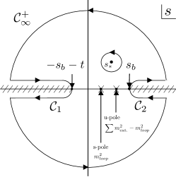
In the complex s-plane, with fixed , we posit the scattering amplitude is holomorphic in and exhibits crossing symmetry, except for poles and cuts along the real axis. We further assume a mild ultraviolet (UV) behavior in the Regge limit as . By subtracting the poles associated with and and denoting the modified amplitude as , we proceed to establish a dispersion relation considering the integration contour in Fig. 1. We further remove those known contributions below the cut off scale where the perturbation theory is valid to improve the dispersion relation:
| (4) |
The forward limit of Eq. 4 presents a subtlety in the presence of gravity, primarily due to the singular first term on the right-hand side (RHS). This term in the forward limit depends on details of quantum gravity. Achieving a finite expression in the forward limit necessitates recognizing the cancellation of singular terms on both sides of equation 4 and careful evaluation of the term, e.g. Reggeization of graviton exchange, which has been explicitly detailed in [6]. Consequently, we can derive a sum rule that relates the infrared observable to the properties of the S-matrix of quantum gravity. However, due to the lack of knowledge of the latter, there is currently no proof of an inequality in contrast to the case for non-gravitational theories.
Interestingly, the positivity of is connected to various versions of the Weak Gravity Conjecture (WGC) mentioned in the introduction. Therefore, we aim to investigate similar phenomena within a more comprehensive framework, specifically the Weinberg-Salam (electroweak) setup.
3 Bounds on electroweak coupled to gravity
In this section, we derive the twice-subtracted dispersion relation for three distinct 2-by-2 scattering processes: , where particles 1 and 2 are incoming, and 3 and 4 are outgoing, with signs indicating photon helicities. The momenta and helicities are defined in the Center of Mass (C.O.M.) frame, as outlined in Ref. [7]. We have utilized the incoming-outgoing convention, considering the summation over four helicity configurations denoted as to manifest crossing for the process. Additionally, for the process, we have specifically taken . We analyze electroweak (EW) minimally coupled to General Relativity (GR) amplitudes at , considering EW and GR regimes separately. In each regime, we take the sum of the results from the QED, Weak, and Higgs sectors,
| (5) |

An example of diagrams of leading contribution in process in GR regime is illustrated in Fig. 2. With the forward scattering at high energy denoted as , the dispersion relation in each regime are derived by,
| (6) |
In the EW sector, the process the amplitude is predominantly governed by the Weak (W and Z)-boson loop. For the process and , the dynamics involve only the W-boson and fermion loops, with the W-boson loop amplitude being dominant.
In the GR regime, the tree level diagrams’ (pole) contribution is offset by the high energy integral of RHS of Eq. 4. Consequently, the one-loop becomes the leading contribution. The process involves only the W-boson and fermion loops. For both the and processes in GR, there are contributions from pure fermion, Weak-boson, and Higgs loops. Additionally, the process includes a unique loop structure formed by Higgs and one line of graviton. It is important to note that the s,u-diagrams arising from this loop structure are subject to infrared (IR) divergence due to the massless nature of the graviton. This problem is addressed by introducing a fictitious graviton mass, assuming the IR divergence is compensated by a soft graviton cloud Ref. [8]. Under this assumption, these diagrams lead to a subleading contribution that is suppressed by the factors . More generally, in the process for all loop types, dominant contributions come from the t-channel. Our results are presented using the Planck scale and the cutoff scale , along with five parameters: the Higgs mass , the Higgs field vacuum expectation value , the electron mass , and the gauge couplings based on the relationships for the W boson mass and for the Z boson mass. The bounds under the assumption of diminishing Higgs mass read,
| (7) | ||||
| (8) | ||||
| (9) |
In the process, it is essential to consider two types of loop corrections stemming from the 3-point vertices and . The first type contributes to the amplitude proportional to the results in the process and is represented by the first factor in equation Eq. (8). The second type of correction results in the last two terms in the equation.
4 Constraints on weak couplings
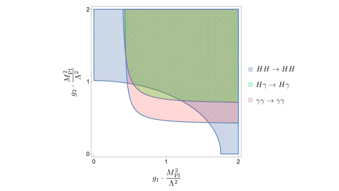
In our initial setup, which assumes a zero Higgs mass, we further hypothesize a large fermion mass, denoted as . Due to this assumption, factors of the order are suppressed. Consequently, from each process, we derive the following constraints for Weak couplings, depicted in Fig. 3.
| (10) | ||||
| (11) | ||||
| (12) |
5 Conclusions
In conclusion, we have found a possible connection between the WGC-like bounds and the positivity in the electroweak-like setup, extending upon the QED analysis. Our study revealed an interesting point: the constraints arising from interactions disallow both couplings to be simultaneously small. Furthermore, the constraints from and interactions prevent either of them from being small on their own. Akin to the magnetic WGC, the constraints suggest that when the coupling constants are small, the effective theory breaks down at a relatively low scale.
Acknowledgement
The results presented in this proceedings are based on an upcoming paper [9]. I would like to thank Katsuki Aoki, Toshifumi Noumi and Junsei Tokuda for their collaboration and comments on the present paper.
References
- [1] C. Cheung and G. N. Remmen, Infrared Consistency and the Weak Gravity Conjecture, JHEP 12 (2014) 087, [1407.7865].
- [2] Y. Hamada, T. Noumi and G. Shiu, Weak Gravity Conjecture from Unitarity and Causality, Phys. Rev. Lett. 123 (2019) 051601, [1810.03637].
- [3] B. Bellazzini, M. Lewandowski and J. Serra, Positivity of Amplitudes, Weak Gravity Conjecture, and Modified Gravity, Phys. Rev. Lett. 123 (2019) 251103, [1902.03250].
- [4] K. Aoki, T. Q. Loc, T. Noumi and J. Tokuda, Is the Standard Model in the Swampland? Consistency Requirements from Gravitational Scattering, Phys. Rev. Lett. 127 (2021) 091602, [2104.09682].
- [5] N. Arkani-Hamed, L. Motl, A. Nicolis and C. Vafa, The String landscape, black holes and gravity as the weakest force, JHEP 06 (2007) 060, [hep-th/0601001].
- [6] J. Tokuda, K. Aoki and S. Hirano, Gravitational positivity bounds, JHEP 11 (2020) 054, [2007.15009].
- [7] L. Alberte, C. de Rham, S. Jaitly and A. J. Tolley, QED positivity bounds, Phys. Rev. D 103 (2021) 125020, [2012.05798].
- [8] T. Noumi and J. Tokuda, Gravitational positivity bounds on scalar potentials, Phys. Rev. D 104 (2021) 066022, [2105.01436].
- [9] K. Aoki, T. Q. Loc, T. Noumi and J. Tokuda, in preparation.