Membrane-in-the-middle optomechanical system and structural frequencies

Abstract

We consider a one-dimensional membrane-in-the-middle model for a cavity that consists of two fixed, perfect mirrors and a mobile dielectric membrane between them that has a constant electric susceptibility. We present a sequence of exact cavity angular frequencies that we call structural angular frequencies and that have the remarkable property that they are independent of the position of the membrane inside the cavity. Furthermore, the case of a thin membrane is considered and simple, approximate, and accurate formulae for the angular frequencies and for the modes of the cavity are obtained. Finally, the cavity electromagnetic potential is numerically calculated and it is found that a multiple scales, analytic solution is an accurate approximation.

I Introduction

Cavity optomechanics investigates the interaction between radiation fields and mechanical oscillators Marquardt.2 . It has enabled the study of mesoscopic and macroscopic systems in the quantum regime and has also proved to be useful to study very rich and complex classical, nonlinear dynamics Thompson -Fig2020 and its relationship to the entanglement dynamics between the mechanical oscillator and the field CND . Moreover, it has found numerous applications such as precision metrology and quantum and classical communication Marquardt.2 and gravitational wave detection gra1 ; gra2 . Further, the mechanical oscillators can be coupled to radiation fields in both the optical and microwave regimes, so they can be implemented as mechanical microwave-optical converters Converter ; MIM2 and have the potential of becoming a link between devices working in different frequency regimes. In fact, cavity optomechanics in the microwave regime has emerged as an area that has the potential to develop new classical electronic devices that can even operate at room temperature Room ; Room2 . Especially relevant for the study, design, and optimization of such devices, a classical electric circuit modeling microwave optomechanics has been developed circuit and it has been successfully tested in an optomechanical system working in the classical regime without fitting parameters MST . Comparison of this classical electric circuit model with the standard quantum treatment permits the establishment of bounds between the quantum and classical regimes and allows the identification of truly quantum features in optomechanical systems circuit . This is especially relevant because an analysis of the nonclassicality of optomechanical phases has revealed that many effects can be reproduced classically QCP .

Cavity optomechanics uses the dependence of the cavity resonance frequency on the position of the mechanical oscillator to couple the electromagnetic field with the mechanical oscillator Marquardt.2 . In addition to this dispersive coupling, one must include both dissipative, and coherent couplings to complete the set of optomechanical interactions Li2019 . The former arises because the cavity decay rate depends on the position of the mechanical oscillator and the latter corresponds to the coupling between cavity modes due to the motion of the mechanical oscillator. In particular, the dissipative coupling can replace the dispersive coupling to perform many tasks such as optomechanical cooling and mechanical sensing, see MOUT and references therein. Typically, the dispersive coupling dominates over the dissipative coupling, so experiments that use the dissipative coupling to perform the aforementioned tasks usually require specific tuning conditions or setups where the dispersive coupling vanishes. Among the several experimental setups that use the dissipative coupling, see MOUT and references therein, the membrane-in-the-middle (MIM) optomechanical setup can present a large dissipative coupling and has the advantage that the resonator and mechanical oscillator can be independently optimized. The latter requires a complex positioning setup that has limited the cavity size and the scalability of such systems, so studies have been carried out to overcome this difficulty and have resulted in similar systems where the membrane is displaced from the middle of the cavity MIM1 . Moreover, it has been shown that such setups can greatly reduce radiation force noise without affecting the coupling between the membrane and the field QDC2 . Actually, the MIM optomechanical set up combines good properties of the cavity, namely, highly reflective mirrors, with good properties of the mechanical oscillator, in particular, very thin, light membranes that can be moved easily by radiation pressure.

In this article we consider a MIM model studied in Law ; 2016 where the membrane is a slab with constant electric susceptibility and establish a sequence of structural angular frequencies that have the remarkable property that they are independent of the position of the membrane inside the cavity. As such, these could lead to new physics in these types of systems, since there would be no dispersive coupling. Furthermore, we consider the case of a thin membrane and obtain approximate analytic formulae with an error term for the angular frequencies and the modes of the cavity. Finally, we show that the potential obtained by solving the appropriate wave equation is accurately approximated by an analytic, multiple scales solution. The MIM model that we consider is a simplification of the models that are used for theoretical studies and in experiments, and it contains some of the essential features of these models. We provide rigorous mathematical results on the angular frequencies, i.e. the resonances, of our model that shed a light in what can happen in experimental setups. We impose a law to the movement of the membrane to simulate the interaction of the electromagnetic field with the membrane, and this is an approximation to the real process. Note moreover, that one dimensional models of a cavity with a membrane that moves according to a law that is given by an external agent are used in other contexts, for example in the dynamical Casimir effect Dodonov .

The article is organized as follows. In Sec. II we present the MIM model and recall some results from 2016 . In Sec. III we present the structural angular frequencies, the approximate cavity angular frequencies for a thin membrane, and compare the potential obtained numerically with the one given by the multiple scales approximation. Finally, in Sec. IV we give our conclusions.

II The membrane-in-the- middle model

In this section we briefly introduce the membrane-in-the-middle (MIM) model used in Law ; 2016 . It was developed to help gain insight into the physics of a mobile membrane interacting with a cavity field.

Consider a one-dimensional cavity with two perfectly conducting, fixed mirrors and a mobile, dielectric membrane in between. We assume that the membrane is a linear, isotropic, non-magnetizable, non-conducting, and uncharged dielectric with thickness $\delta_{0}$ when it is at rest. In particular, the membrane is not restricted to small displacements near an equilibrium position. Figure 1 gives a schematic representation of the system. The boundaries of the fixed mirrors are located at $x=0$ and $x=L$. We denote by $q(t)$ the midpoint of the membrane and refer to it as the position of the membrane. Moreover, $\chi(x)$ is the electric susceptibility of the membrane and we assume that it is a nonnegative, piecewise continuous function with a piecewise continuous derivative such that $\chi[x-q(t)]=0$ if $|x-q(t)|\geq\delta_{0}/2$. Also, the dielectric function of the membrane is $\varepsilon:=1+4\pi\chi$ and we use Gaussian units. For a study of the coupled dynamics of the electromagnetic field inside the cavity and the moving membrane by means of self consistent, coupled equations see PhysicaScripta .

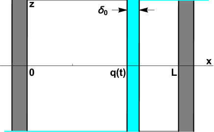
Figure 1: Schematic of the MIM model. The interior of the cavity goes from $x=0$ to $x=L$ and the outer slabs correspond to the fixed, perfectly conducting mirrors. The mobile dielectric membrane is the slab inside the cavity, has thickness $\delta_{0}$, and its midpoint is $q(t)$.

The electric and magnetic fields inside the cavity are derived from a vector potential

$$\mathbf{A}(x,t)\ =\ A_{0}(x,t)\mathbf{\hat{z}},$$ (1)

where $\mathbf{\hat{z}}$ is the unit vector in the direction of the positive $z$-axis.

Let $\nu_{0}$ be a characteristic frequency of the electromagnetic field (there are no decay rates here), $\lambda_{0}=c/\nu_{0}$ with $c$ the speed of light in vacuum the corresponding characteristic wavelength, $A_{00}$ a characteristic value of $A_{0}(x,t)$, and $\nu_{\mbox{\tiny osc}}^{-1}$ the time-scale in which $q(t)$ varies appreciably. We measure time in units of $\nu_{0}^{-1}$ and lengths in units of $\lambda_{0}$, so the dimensionless time $\tau$ and position $\xi$ are

$$\tau=\nu_{0}t,\,\qquad\xi=\frac{x}{\lambda_{0}}.$$ (2)

Also, we introduce following nondimensional quantities:

$$\xi_{L} = \frac{L}{\lambda_{0}},\quad\tilde{\chi}\left[\xi-\tilde{q}(\tau)\right]=\chi\left[\lambda_{0}\left[\xi-\tilde{q}(\tau)\right]\right]\ ,$$ (3)

$$\tilde{\delta}_{0} = \frac{\delta_{0}}{\lambda_{0}}\ ,\quad\tilde{\epsilon}\left[\xi-\tilde{q}(\tau)\right]=1+4\pi\tilde{\chi}\left[\xi-\tilde{q}(\tau)\right]\ ,$$ (4)

$$\tilde{q}(\tau) = \frac{q(\nu_{0}^{-1}\tau)}{\lambda_{0}},\quad\epsilon_{\mbox{\tiny pert}}=\frac{\nu_{\mbox{\tiny osc}}}{\nu_{0}}\ ,$$ (6)

$$\tilde{A}_{0}(\xi,\tau) = \frac{A_{0}(\lambda_{0}\xi,\nu_{0}^{-1}\tau)}{A_{00}}.$$ (7)

The quantities $\xi_{L}$ and $\tilde{\delta}_{0}$ are the nondimensional length of the cavity and the nondimensional thickness of the membrane, while $\tilde{q}(\tau)$ is the nondimensional position of the membrane. Also, $\tilde{\chi}\left[\xi-\tilde{q}(\tau)\right]$ and $\tilde{\epsilon}\left[\xi-\tilde{q}(\tau)\right]$ are the electric susceptibility and the dielectric function of the membrane in terms of the nondimensional argument $[\xi-\tilde{q}(\tau)]$, respectively, and $\tilde{A}_{0}(\xi,\tau)$ is the non-dimensional potential. The parameter $\epsilon_{\mbox{\tiny pert}}$ is the quotient of the time-scale, $1/\nu_{0},$ in which the electromagnetic field evolves appreciably divided by the time-scale, $1/\nu_{\mbox{\tiny osc}},$ in which the membrane moves appreciably. In the electromagnetic MIM model in Thompson , taking the values from Table 1 one has $\nu_{0}=5.63\times 10^{14}$ Hz, $\nu_{\mbox{\tiny osc}}=10^{5}$ Hz, and, consequently, $\epsilon_{\mbox{\tiny pert}}=1.8\times 10^{-10}.$ In the experiment MST in the microwave regime one has $\nu_{0}=5.153$ GHz, $\nu_{\mbox{\tiny osc}}=15.129$ MHz, and, consequently, $\epsilon_{\mbox{\tiny pert}}=2.936\times 10^{-3}.$

The general equation that governs the dynamics of $\tilde{A}_{0}(\xi,\tau)$ without any restriction on the values of the velocity and the acceleration of the membrane was obtained in PhysicaScripta by means of a relativistic analysis. To first order in $\tilde{q}^{\prime}(\tau)$ and $\tilde{q}^{\prime\prime}(\tau)$, the equation is given by

$$\frac{\partial^{2}\tilde{A}_{0}}{\partial\xi^{2}}(\xi,\tau) = \tilde{\epsilon}\left[\xi-\tilde{q}(\tau)\right]\frac{\partial^{2}\tilde{A}_{0}}{\partial\tau^{2}}(\xi,\tau)$$ (10)

$$+8\pi\tilde{q}^{\prime}(\tau)\tilde{\chi}\left[\xi-\tilde{q}(\tau)\right]\frac{\partial^{2}\tilde{A}_{0}}{\partial\xi\partial\tau}(\xi,\tau)$$

$$+4\pi\tilde{q}^{\prime\prime}(\tau)\tilde{\chi}\left[\xi-\tilde{q}(\tau)\right]\frac{\partial\tilde{A}_{0}}{\partial\xi}(\xi,\tau)\ .$$

The boundary conditions that correspond to the perfectly conducting mirrors are

$$\tilde{A}_{0}(0,\tau)\ =\ 0\ ,\ \ \tilde{A}_{0}(\xi_{L},\tau)\ =\ 0\ .$$ (11)

II.1 The angular frequencies and the modes of the cavity

We now present results from 2016 on the evolution of the potential in the case where the membrane is fixed.

Assume that the membrane is fixed at some point inside the cavity,

$$\tilde{q}(\tau)=\tilde{q}_{0}\ \in\left[\frac{\tilde{\delta}_{0}}{2},\ \xi_{L}-\frac{\tilde{\delta}_{0}}{2}\right]\ .$$ (12)

Since the velocity and the acceleration of the membrane are zero, (10) reduces to the wave equation,

$$\frac{\partial^{2}\tilde{A}_{0}}{\partial\xi^{2}}(\xi,\tau) = \tilde{\epsilon}\left(\xi-\tilde{q}_{0}\right)\frac{\partial^{2}\tilde{A}_{0}}{\partial\tau^{2}}(\xi,\tau)\ .$$ (13)

We look for solutions to (13) that are periodic in time,

$$\tilde{A}_{0}(\xi,\tau)=e^{\pm i\omega(\tilde{q}_{0})\tau}G(\xi,\tilde{q}_{0}).$$ (14)

The cavity has a countable set of nondimensional angular frequencies, $\{\omega_{n}(\tilde{q}_{0})\}_{n=1}^{+\infty}$, with the associated set of cavity modes $\{G_{n}(\xi,\tilde{q}_{0})\}_{n=1}^{+\infty}$ consisting of multiplicity one eigenfunctions that are solutions to the following boundary value problem

$$\frac{\partial^{2}G_{n}}{\partial\xi^{2}}(\xi,\tilde{q}_{0}) = -\omega_{n}(\tilde{q}_{0})^{2}\tilde{\epsilon}(\xi-\tilde{q}_{0})G_{n}(\xi,\tilde{q}_{0})\ ,$$ (15)

$$G_{n}(0,\tilde{q}_{0}) = 0\ ,\quad G_{n}(\xi_{L},\tilde{q}_{0})=0\ .$$ (17)

We order the angular frequencies in such a way that $\omega_{m}(\tilde{q}_{0})<\omega_{n}(\tilde{q}_{0})$ if $m<n$. Moreover, $\omega_{n}(\tilde{q}_{0})>0,$ and $\lim_{n\to\infty}\omega_{n}(\tilde{q}_{0})=\infty.$ In addition, there are no crossings: if $n\neq m$, then $\omega_{n}(\tilde{q}_{0})\neq\omega_{m}(\tilde{q}_{0})$ for all $\tilde{q}_{0}\ \in\left[\frac{\tilde{\delta}_{0}}{2},\ \xi_{L}-\frac{\tilde{\delta}_{0}}{2}\right].$ The set of cavity modes is an orthonormal basis of real-valued functions in the Hilbert space $L^{2}_{\tilde{q}_{0}}$ of all complex-valued, Lebesgue square-integrable functions on $(0,\xi_{L})$ with the scalar product

$$\left(f,g\right)_{\tilde{\varepsilon}}:=\int_{0}^{\xi_{L}}d\xi\ \tilde{\epsilon}(\xi-\tilde{q}_{0})\overline{f(\xi,\tilde{q}_{0})}g(\xi,\tilde{q}_{0}).$$

II.2 The multiple scales approximation

Following 2016 , we consider now the situation where the membrane is allowed to move.

For each fixed $\tau$ we denote by $\{\omega_{n}[\tilde{q}(\tau)]\}_{n=1}^{+\infty}$  the instantaneous angular frequencies of the cavity and by $\{G_{n}[\xi,\tilde{q}(\tau)]\}_{n=1}^{+\infty}$ the associated set of instantaneous modes. For simplicity we refer to them as the cavity angular frequencies and modes. Using that for each fixed $\tau$ the modes of the cavity are an orthonormal basis, we expand $\tilde{A}_{0}(\xi,\tau)$ as

$$\tilde{A}_{0}(\xi,\tau) = \sum_{n=1}^{+\infty}c_{n}(\tau)G_{n}[\xi,\tilde{q}(\tau)].$$ (18)

Introducing (18) into (10) we deduce the equations for the coefficients $c_{n}(\tau)$:

$$c_{m}^{\prime\prime}(\tau)+\omega_{m}[\tilde{q}(\tau)]^{2}c_{m}(\tau)=$$ (19)

$$-\sum_{n=1}^{+\infty}\Gamma_{mn}[\tilde{q}(\tau)]\Big{[}\ 2\tilde{q}^{\prime}(\tau)c_{n}^{\prime}(\tau)+\tilde{q}^{\prime\prime}(\tau)c_{n}(\tau)\ \Big{]}\ .$$ (20)

Here we introduced the following quantities:

$$\Omega_{mn}\left[\tilde{q}(\tau)\right] = \int_{0}^{\xi_{L}}d\xi\ \tilde{\epsilon}\left[\xi-\tilde{q}(\tau)\right]G_{m}\left[\xi,\tilde{q}(\tau)\right]\times$$ (22)

$$\qquad\qquad\frac{\partial G_{n}}{\partial\tilde{q}(\tau)}\left[\xi,\tilde{q}(\tau)\right]\ ,$$

$$\theta_{mn}\left[\tilde{q}(\tau)\right] = \int_{0}^{\xi_{L}}d\xi\ 4\pi\tilde{\chi}\left[\xi-\tilde{q}(\tau)\right]G_{m}\left[\xi,\tilde{q}(\tau)\right]\times$$ (25)

$$\qquad\qquad\frac{\partial G_{n}}{\partial\xi}\left[\xi,\tilde{q}(\tau)\right]\ ,$$

$$\Gamma_{mn}\left[\tilde{q}(\tau)\right] = \Omega_{mn}\left[\tilde{q}(\tau)\right]+\theta_{mn}\left[\tilde{q}(\tau)\right]\ .$$ (27)

The system of ordinary differential equations (19) for the expansions coefficients $c_{n}(\tau)$ in (18) is equivalent to the wave equation (10). As it is the case with (10), the system (19) is accurate to first order in $\tilde{q}^{\prime}(\tau)$ and $\tilde{q}^{\prime\prime}(\tau)$.

We make the following four assumptions 2016 :

1. The functions $\tilde{q}^{\prime}(\tau)$ and $\tilde{q}^{\prime\prime}(\tau)$ are small. These conditions are necessary in order that the system (19) is correct to first order in $\tilde{q}^{\prime}(\tau)$ and $\tilde{q}^{\prime\prime}(\tau).$

2. $0<\epsilon_{\mbox{\tiny pert}}\ll 1$. This assumption implies that there are two clearly defined and separate time-scales: a fast time-scale $1/\nu_{0}$ in which the electromagnetic field evolves and a slow time-scale $1/\nu_{\mbox{\tiny osc}}$ in which the membrane moves.

3. The initial conditions for the coefficients $c_{m}(\tau)$ of the modes are

   $$c_{m}(0) = g_{0N}\delta_{mN}\ ,\quad c_{m}^{\prime}(0)=g_{1N}\delta_{mN}\ ,$$ (28)

   where $g_{0N}$ and $g_{1N}$ are real numbers and $N$ is a fixed, positive integer. These initial conditions indicate that only mode $N$ is initially excited.

4. The membrane is initially at rest, i.e., $\tilde{q}^{\prime}(0)=0$.

These assumptions correspond to the following physical situation: the membrane starts to move from rest and the field is initially found in one of the modes of the cavity.

Let

$$t_{1N}(\tau) = \int_{0}^{\tau}\omega_{N}\left[\tilde{q}(\rho)\right]d\rho\ ,$$ (29)

$$\alpha_{N}\left[\tilde{q}(\tau)\right] = \sqrt{\frac{\omega_{N}\left[\tilde{q}(0)\right]}{\omega_{N}\left[\tilde{q}(\tau)\right]}}\ \mbox{exp}\left\{-\int_{\tilde{q}(0)}^{\tilde{q}(\tau)}dy\ \Gamma_{NN}(y)\right\}\ ,$$ (30)

$$b_{N0} = \left|\frac{g_{0N}}{2}+\frac{ig_{1N}}{2\omega_{N}\left[\tilde{q}(0)\right]}\right|\ ,$$ (32)

$$\Theta_{N0} = \mbox{arg}\left[\frac{g_{0N}}{2}+\frac{ig_{1N}}{2\omega_{N}\left[\tilde{q}(0)\right]}\right]\ .$$ (34)

Then, the multiple scales solution is given by 2016

$$\tilde{A}_{0}^{(2)}(\xi,\tau) = \alpha_{N}\left[\tilde{q}(\tau)\right]b_{N0}e^{-i\left[t_{1N}(\tau)-\Theta_{N0}\right]}G_{N}[\xi,\tilde{q}(\tau)]\times$$ (38)

$$\left\{1+i\tilde{q}^{\prime}(\tau)\frac{\omega_{N}^{\prime}\left[\tilde{q}(\tau)\right]}{4\omega_{N}\left[\tilde{q}(\tau)\right]^{2}}\right\}+$$

$$\alpha_{N}\left[\tilde{q}(\tau)\right]b_{N0}e^{-i\left[t_{1N}(\tau)-\Theta_{N0}-\pi/2\right]}\tilde{q}^{\prime}(\tau)\times$$

$$\sum_{m=1\atop m\not=N}^{+\infty}\frac{2\Gamma_{mN}\left[\tilde{q}(\tau)\right]\omega_{N}\left[\tilde{q}(\tau)\right]}{\omega_{m}\left[\tilde{q}(\tau)\right]^{2}-\omega_{N}\left[\tilde{q}(\tau)\right]^{2}}G_{m}[\xi,\tilde{q}(\tau)]+$$

$$c.c.$$ (39)

Observe that an electromagnetic field initially in mode $N$ will follow mode $N$, provided that the membrane moves slowly. In addition, only modes  $n\not=N$  with $\omega_{n}[\tilde{q}(\tau)]$ in a small band around $\omega_{N}[\tilde{q}(\tau)]$ can have a non-negligible excitation.

III The case of a slab membrane

In this section we present our new results. We consider the particular case where the electric susceptibility is

$$\tilde{\chi}(\xi-\tilde{q}_{0}) = \left\{\begin{array}[]{cc}\chi_{0}&\mbox{if}\ \ |\xi-\tilde{q}_{0}|\ <\ \frac{\tilde{\delta}_{0}}{2}\ ,\cr 0&\mbox{elsewhere.}\end{array}\right.$$ (42)

We assume that the membrane is fixed at $\tilde{q}_{0}$ as in (12) and we introduce the following convenient notation

$$\alpha:=\sqrt{1+4\pi\chi_{0}},\quad\beta:=\frac{\tilde{q}_{0}-\tilde{\delta}_{0}/2}{\xi_{L}}.$$ (43)

Hence,

$$\tilde{q}_{0}-\tilde{\delta}_{0}/2=\beta\xi_{L},\qquad 0<\beta<1-\frac{\tilde{\delta}_{0}}{\xi_{L}}.$$ (44)

Imposing that the Dirichlet boundary condition is satisfied at $\xi=0$ and $\xi=\xi_{L}$ and the continuity of $G_{n}(\xi,\tilde{q}_{0})$ and its first partial derivative with respect to $\xi$ at the boundaries of the membrane $\xi=\tilde{q}_{0}\pm\tilde{\delta}_{0}/2$, we calculate explicitly the modes in terms of elementary functions and we obtain an implicit equation for the calculation of the angular frequencies of the cavity. Namely,

$$G_{n}(\xi,\tilde{q}_{0})=\frac{1}{\sqrt{\mathcal{N}_{n}(\tilde{q}_{0})}}\widehat{G}_{n}(\xi,\tilde{q}_{0}),$$ (45)

with

$$\widehat{G}_{n}(\xi,\tilde{q}_{0})=\sin[\omega_{n}(\tilde{q}_{0})\xi]\quad\mathrm{if}\quad 0\leq\xi\leq\tilde{q}_{0}-\frac{\tilde{\delta}_{0}}{2},$$ (46)

and

$$\widehat{G}_{n}(\xi,\tilde{q}_{0}) = \cos[\omega_{n}(\tilde{q}_{0})\alpha(\xi-\xi_{L}\beta)]\sin[\xi_{L}\omega_{n}(\tilde{q}_{0})\beta]$$ (48)

$$+\frac{1}{\alpha}\sin[\omega_{n}(\tilde{q}_{0})\alpha(\xi-\xi_{L}\beta)]\cos[\xi_{L}\omega_{n}(\tilde{q}_{0})\beta]$$

$$\mathrm{if} \left|\xi-\tilde{q}_{0}\right|\leq\tilde{\delta}_{0}/2,$$ (49)

and

$$\widehat{G}_{n}(\xi,\tilde{q}_{0})$$ (50)

$$= \frac{1}{4\alpha}\Bigg{\{}(1+\alpha)^{2}\sin\left\{\omega_{n}(\tilde{q}_{0})\left[\xi+\tilde{\delta}_{0}(\alpha-1)\right]\right\}$$ (54)

$$-(\alpha-1)^{2}\sin\left\{\omega_{n}(\tilde{q}_{0})\left[\xi-\tilde{\delta}_{0}(\alpha+1)\right]\right\}$$

$$-(\alpha^{2}-1)\sin\left\{\omega_{n}(\tilde{q}_{0})\left[\xi+\tilde{\delta}_{0}(\alpha-1)-2\xi_{L}\beta\right]\right\}$$

$$+(\alpha^{2}-1)\sin\left\{\omega_{n}(\tilde{q}_{0})\left[\xi-\tilde{\delta}_{0}(\alpha+1)-2\xi_{L}\beta\right]\right\}\Bigg{\}}$$

$$\mathrm{if} \xi\geq\tilde{q}_{0}+\tilde{\delta}_{0}/2.$$ (55)

The coefficient $\mathcal{N}_{n}(\tilde{q}_{0})$ is obtained by requiring that ${G}_{n}(\xi,\tilde{q}_{0})$ be normalized to one. It is given by

$$\mathcal{N}_{n}(\tilde{q}_{0}):=\int_{0}^{\xi_{L}}\,\tilde{\varepsilon}(\xi-\tilde{q}_{0})|\widehat{G}_{n}(\xi,\tilde{q}_{0})|^{2}d\xi,$$ (56)

and it can be evaluated explicitly using (56) and a symbolic programming language like Mathematica. The expression is, however, rather complicated and we decided not to include it. Instead, in the numerical computations we evaluate it whenever it is needed. Moreover, we have the following implicit equation to evaluate the angular frequencies of the cavity:

$$\begin{array}[]{l}-(\alpha-1)^{2}\sin\left\{\omega(\tilde{q}_{0})\left[\xi_{L}-\tilde{\delta}_{0}(\alpha+1)\right]\right\}\\ -2(\alpha^{2}-1)\cos\left[\omega(\tilde{q}_{0})\left(\xi_{L}-\tilde{\delta}_{0}-2\xi_{L}\beta\right)\right]\sin\left[\omega(\tilde{q}_{0})\tilde{\delta}_{0}\alpha\right]\\ +(\alpha+1)^{2}\sin\left\{\omega(\tilde{q}_{0})\left[\xi_{L}+\tilde{\delta}_{0}(\alpha-1)\right]\right\}=0.\end{array}$$ (57)

Recall that the angular frequencies of the cavity are positive, so we have to look for positive solutions to (57). Below we find an explicit solution to (57). For further explicit solutions see the next section.

Assume that the membrane is in the middle of the cavity. Then,

$$\tilde{q}_{0}=\frac{\xi_{L}}{2}=\xi_{L}\beta+\frac{\tilde{\delta}_{0}}{2},$$

and

$$2\xi_{L}\beta=\xi_{L}-\tilde{\delta}_{0}.$$ (58)

Using (58), it follows from a simple computation that (57) can be written as,

$$\begin{array}[]{l}(\alpha^{2}+1)\cos[\omega(\tilde{q}_{0})(\xi_{L}-\tilde{\delta}_{0})]\sin[\omega(\tilde{q}_{0})\tilde{\delta}_{0}\alpha]-\\ \\ (\alpha^{2}-1)\sin[\omega(\tilde{q}_{0})\tilde{\delta}_{0}\alpha]+\\ \\ 2\alpha\sin[\omega(\tilde{q}_{0})(\xi_{L}-\tilde{\delta}_{0})]\cos[\omega(\tilde{q}_{0})\tilde{\delta}_{0}\alpha]=0.\end{array}$$ (59)

Take

$$\omega(\tilde{q}_{0})=\omega_{n}(\tilde{q}_{0}):=\frac{1}{\tilde{\delta}_{0}\alpha}(2n+1)\frac{\pi}{2},\qquad n=0,1,\dots.$$ (60)

Then, (59) reduces to,

$$\cos[\omega_{n}(\tilde{q}_{0})(\xi_{L}-\tilde{\delta}_{0})]=\frac{\alpha^{2}-1}{\alpha^{2}+1}=\frac{4\pi\chi_{0}}{2+4\pi\chi_{0}}.$$ (61)

Denote,

$$\gamma:=\arccos\left[\frac{4\pi\chi_{0}}{2+4\pi\chi_{0}}\right].$$

Then, by (60), (61) is equivalent to,

$$\tilde{\delta}_{0}=\tilde{\delta}_{0,n}:=\xi_{L}\frac{(2n+1)\pi}{(2n+1)\pi+2\alpha\gamma},\qquad n=0,1,\dots.$$ (62)

Further, introducing (62) into (60) we get,

$$\omega(\tilde{q}_{0})=\omega_{n}(\tilde{q}_{0})=\frac{1}{\xi_{L}}\left[\gamma+\frac{1}{\alpha}(2n+1)\frac{\pi}{2}\right],\quad n=0,1,\dots.$$ (63)

Hence, we have proven that, for $\tilde{q}_{0}=\xi_{L}/2,$ the angular frequencies (63) are explicit solutions to (57) for the widths of the membrane given by (62).

III.1 Structural angular frequencies

In this subsection we give explicitly a sequence of structural angular frequencies that have the remarkable property that they are independent of the position of the membrane inside the cavity. More precisely, for each fixed value of the length of the cavity and each fixed value of the electric susceptibility of the membrane, we find a sequence of widths of the membrane such that, for each width in the sequence, there is a cavity angular frequency that is independent of the position of the membrane inside the cavity, i.e., such that it is a cavity angular frequency for all positions of the membrane inside the cavity. Furthermore, these cavity angular frequencies are the only ones that have the remarkable property of being independent of the position of the membrane inside the cavity.

Theorem Let us consider a fixed $\xi_{L}>0$ and a fixed $\chi_{0}>0.$ For $k=1,2,\dots$ and $n=1,2,\dots$ we define

$$\omega_{n,k}:=\frac{(n\alpha+k)\pi}{\xi_{L}\alpha},$$ (64)

and

$$\tilde{\delta}_{0,n,k}:=\xi_{L}\frac{k}{n\alpha+k}<\xi_{L}.$$ (65)

Then, $\omega_{n,k}$ is a solution to (57), i.e., it is one of the cavity’s angular frequencies with $\tilde{\delta}_{0}=\tilde{\delta}_{0,n,k}$ as in (65) with the same $n,k$ for all $\tilde{\delta}_{0}/2<\tilde{q}_{0}<\xi_{L}-\tilde{\delta}_{0}/2$. Moreover, the only cavity angular frequencies that satisfy (57) with a fixed $\tilde{\delta}_{0}\in(0,\xi_{L})$ for all $\tilde{q}_{0}$ in a nontrivial interval contained in $(\tilde{\delta}_{0}/2,\xi_{L}-\tilde{\delta}_{0}/2)$ are the ones given by (64) with $\tilde{\delta}_{0}=\tilde{\delta}_{0,n,k}$ given by (65) with the same $n,k.$

Proof: Let us take in (57)

$$\omega=\frac{k\pi}{\alpha\tilde{\delta}_{0}},\qquad k=1,2,\dots.$$ (66)

Then,

$$\sin(\omega\tilde{\delta}_{0}\alpha)=0,$$

and (57) simplifies to

$$\begin{array}[]{l}(\alpha+1)^{2}\sin\left\{\omega\left[\xi_{L}+\tilde{\delta}_{0}(\alpha-1)\right]\right\}\\ \\ =(\alpha-1)^{2}\sin\left\{\omega\left[\xi_{L}-\tilde{\delta}_{0}(\alpha+1)\right]\right\}.\end{array}$$ (67)

Further, introducing (66) into (67) we get

$$4\alpha\sin\left(\omega\xi_{L}-k\frac{\pi}{\alpha}\right)=0.$$ (68)

Hence, for $k,n=1,2,\dots$ one has

$$w=\omega_{n,k}:=\frac{(n\alpha+k)\pi}{\xi_{L}\alpha}.$$ (69)

Finally, using (66) and (69) we obtain (65). Note that the case $n=0$ in (64), (65) is excluded because we need that $\tilde{\delta}_{0}<\xi_{L}.$

Now, assume that $w>0$ satisfies (57) for a fixed $\xi_{L}$ and that (57) holds for all $\tilde{q}_{0}\in(a,b)\subset(\tilde{\delta}_{0}/2,\xi_{L}-\tilde{\delta}_{0}/2)$ for some $a<b$. Then, we can take the derivative of both sides of (57) with respect to $\beta$ to obtain that

$$\sin(\omega\tilde{\delta}_{0}\alpha)=0.$$

Hence, (66) holds and, as above, we prove (64) and (65).

$\Box$

Note that keeping $k$ fixed in (65) and taking $n$ large we can make the membrane as thin as we wish, but by (64) the corresponding structural angular frequency becomes very large.

We proceed to prove that the structural angular frequencies are always larger than the fundamental angular frequency $\omega_{1}(\tilde{q}_{0})$ with $\tilde{q_{0}}\in\left[\frac{\tilde{\delta}_{0}}{2},\ \xi_{L}-\frac{\tilde{\delta}_{0}}{2}\right]$ and that they are separated from the fundamental frequency by as least $\pi/(\xi_{L}\alpha)$. This is a simple consequence of the min-max principle in the theory of selfadjoint operators in Hilbert space. We denote by $L^{2}(0,\xi_{L})$ the standard space of Lebesgue square-integrable functions on $(0,\xi_{L}).$ As mentioned in Section  II.1, we denote by $L^{2}_{\tilde{q}_{0}}$ with $\tilde{q}_{0}\in\left[\frac{\tilde{\delta}_{0}}{2},\ \xi_{L}-\frac{\tilde{\delta}_{0}}{2}\right]$ the space $L^{2}(0,\xi_{L})$ endowed with the scalar product

$$(\phi,\psi)_{L^{2}_{\tilde{q}_{0}}}:=\int_{0}^{\xi_{L}}d\xi\ \tilde{\epsilon}(\xi-\tilde{q}_{0})\overline{\phi(\xi)}\psi(\xi).$$

By $H_{2}$ we designate the second Sobolev space on $(0,\xi_{L})$ and by $H_{1,0}$ the first Sobolev space of functions on $(0,\xi_{L})$ that vanish for $\xi=0$ and $\xi=\xi_{L}.$ For the definition and properties of these spaces see Sobolev . We define the following selfadjoint, positive operator $\mathbb{A}_{\tilde{q}_{0}}$ in $L^{2}_{\tilde{q}_{0}},$

$$\mathbb{A}_{\tilde{q}_{0}}\phi:=-\frac{1}{\tilde{\varepsilon}(\xi-\tilde{q}_{0})}\frac{d^{2}}{d\xi^{2}}\phi,$$

with the following domain,

$$D\left(\mathbb{A}_{\tilde{q}_{0}}\right):=H_{2}\cap H_{1,0}.$$

As proved in 2016 the spectrum of $\mathbb{A}_{\tilde{q}_{0}}$ consists of eigenvalues of multiplicity one that coincide with the square of the angular frequencies. Moreover, the quadratic form of $\mathbb{A}_{\tilde{q}_{0}}$ is given by

$$h_{\tilde{q}_{0}}(\phi,\psi):=\int_{0}^{\xi_{L}}d\xi\overline{\phi^{\prime}(\xi)}\psi^{\prime}(\xi),$$

with domain

$$D(h_{\tilde{q}_{0}}):=H_{1,0}.$$

Let us denote by $\mathbb{B}$ the Dirichlet Laplacian in $L^{2}(0,\xi_{L}),$

$$\mathbb{B}\phi:=-\frac{d^{2}}{d\xi^{2}}\phi,$$

with domain

$$D\left(\mathbb{B}\right):=H_{2}\cap H_{1,0}.$$

$\mathbb{B}$ is selfadjoint, positive, and its spectrum, $\{(\frac{k\pi}{\xi_{L}})^{2}\}_{k=1}^{\infty}$, consists of the eigenvalues of multiplicity one. Further, the quadratic form of $\mathbb{B}$ is given by,

$$h_{\mathbb{B}}(\phi,\psi):=\int_{0}^{\xi_{L}}d\xi\overline{\phi^{\prime}(\xi)}\psi^{\prime}(\xi),$$

with domain

$$h_{\mathbb{B}}:=H_{1,0}.$$

Note that,

$$h_{\tilde{q}_{0}}(\phi,\psi)=h_{\mathbb{B}}(\phi,\psi),\qquad\phi,\psi\in H_{1,0},$$

but that $\mathbb{A}_{\tilde{q}_{0}}$ and $\mathbb{B}$ act in different Hilbert spaces, namely, in $L^{2}_{\tilde{q}_{0}}$ and $L^{2}(0,\xi_{L})$, respectively. By the min-max principle (see Theorem XIII.2 in page 78 of rs )

$$\begin{array}[]{l}\omega_{1}(\tilde{q}_{0})^{2}=\inf_{\phi\in H_{1,0},\phi\neq 0}\frac{\left(\phi^{\prime},\phi^{\prime}\right)_{L^{2}(0,\xi_{L})}}{\|\phi\|^{2}_{L^{2}_{\tilde{q}_{0}}}}\\ \leq\inf_{\phi\in H_{1,0},\phi\neq 0}\frac{\left(\phi^{\prime},\phi^{\prime}\right)_{L^{2}(0,\xi_{L})}}{\|\phi\|^{2}_{L^{2}(0,\xi_{L})}}=(\frac{\pi}{\xi_{L}})^{2},\end{array}$$ (70)

where we use that

$$\|\phi\|_{L^{2}_{\tilde{q}_{0}}}\geq\|\phi\|_{L^{2}(0,\xi_{L})},$$

and that $(\frac{\pi}{\xi_{L}})^{2}$ is the smallest eigenvalue of $\mathbb{B}$. Then, by (64) and (70), for $k,n=1,2,\dots,$

$$\begin{array}[]{l}\omega_{n,k}\geq\omega_{1,1}=\frac{\pi}{\xi_{L}}+\frac{\pi}{\xi_{L}\alpha}\geq\omega_{1}(\tilde{q}_{0})+\frac{\pi}{\xi_{L}\alpha},\\ \tilde{q}_{0}\in\left[\frac{\tilde{\delta}_{0}}{2},\ \xi_{L}-\frac{\tilde{\delta}_{0}}{2}\right].\end{array}$$ (71)

Hence, the structural angular frequencies are strictly larger that the fundamental angular frequency $\omega_{1}(\tilde{q}_{0})$ and they are separated from the fundamental frequency by at least $\frac{\pi}{\xi_{L}\alpha}.$

In Figure 2 we show the lowest $29$ angular frequencies of the cavity computed numerically using the implicit equation (57) as a function of the position of the left side of the membrane. We take $\tilde{\delta}_{0}=1/3,\alpha=2,$ and $\xi_{L}=2.$ For these values (64) gives the sequence of structural angular frequencies $\omega_{5l,2l}=3\pi l,l=1.\dots$ The lowest four structural angular frequencies appear as horizontal straight lines in Figure 2 .

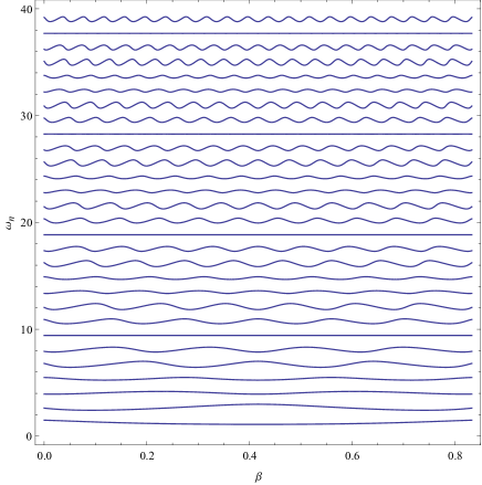
Figure 2: Numerical computation of the lowest $29$ angular frequencies using the implicit equation (57), as a function of the parameter $\beta:=\frac{\tilde{q}_{0}-\tilde{\delta}_{0}/2}{\xi_{L}}$. The width of the membrane is $\tilde{\delta}_{0},$ the position of the left side of the membrane is $\tilde{q}_{0}-\frac{1}{2}\tilde{\delta}_{0},$ and the length of the cavity is $\xi_{L}.$ Note that, $0<\beta<1-\frac{\tilde{\delta}_{0}}{\xi_{L}}.$ We have taken $\xi_{L}=2,\tilde{\delta}_{0}=\frac{1}{3},$ and $\alpha:=\sqrt{1+4\pi\chi_{0}}=2.$ Note that the first four structural angular frequencies appear as straight horizontal lines.

III.2 The case of a thin membrane

In this subsection we consider approximate solutions when the width $\tilde{\delta}_{0}$ of the membrane is small. This case is important, as often in the experiments, and in the applications the width of the membrane is is very small. For example, in Thompson the width of the membrane in units of the cavity’s length is $\tilde{\delta}_{0}=0.74\times 10^{-6}.$ Below we denote by $G_{n,l}(\xi,\tilde{q}_{0})$ and $\widehat{G}_{n,l}(\xi,\tilde{q}_{0}),$ respectively, the approximate normalized solution and the approximate unnormalized solution to first order in $\tilde{\delta}_{0}$. Further we denote by ${\mathcal{N}_{n,l}(\tilde{q}_{0})}$ the norming coefficient of the approximate normalized solution $G_{n,l}(\xi,\tilde{q}_{0})$. Approximating (50) to first order in $\tilde{\delta}_{0}$ (note that (46) and (48) do not depend explicitly on $\tilde{\delta}_{0}$), we obtain

$$G_{n,l}(\xi,\tilde{q}_{0})=\frac{1}{\sqrt{\mathcal{N}_{n,l}(\tilde{q}_{0})}}\widehat{G}_{n,l}(\xi,\tilde{q}_{0}),$$ (72)

where $\widehat{G}_{n,l}(\xi,\tilde{q}_{0})$ is exactly equal to $\widehat{G}_{n}(\xi,\tilde{q}_{0})$ in (46) and (48) for $\xi\leq\tilde{q}_{0}+\tilde{\delta}_{0}/2$ and

$$\begin{array}[]{l}\widehat{G}_{n,l}(\xi,\tilde{q}_{0})=\sin[\omega_{n}(\tilde{q}_{0})\xi]+\frac{1}{2}\tilde{\delta}_{0}\Big{\{}\omega_{n}(\tilde{q}_{0})(-1+\alpha^{2})\\ \\ \cos[\omega_{n}(\tilde{q}_{0})\xi]+(1-\alpha^{2})\omega_{n}(\tilde{q}_{0})\cos\left[\omega_{n}(\tilde{q}_{0})(\xi-2\xi_{L}\beta)\right]\Big{\}},\\ \\ \mathrm{for}\quad\tilde{q}_{0}+\frac{\tilde{\delta}_{0}}{2}\leq\xi\leq\xi_{L}.\end{array}$$ (73)

By the Taylor expansion, the error made by approximating (50) by (73) is smaller than $\frac{1}{2}\alpha(\alpha^{2}-1)[\omega_{n}(\tilde{q}_{0})\,\tilde{\delta}_{0}]^{2}.$ The norming coefficient $\mathcal{N}_{n,l}$ is defined as

$$\mathcal{N}_{n,l}(\tilde{q}_{0}):=\int_{0}^{\xi_{L}}\,\tilde{\varepsilon}(\xi-\tilde{q}_{0})|\widehat{G}_{n,l}(\xi,\tilde{q}_{0})|^{2}d\xi,$$ (74)

$$\begin{array}[]{l}\displaystyle\sqrt{\mathcal{N}_{n,l}(\tilde{q}_{0})}=\frac{1}{2}\Bigg{\{}2\xi_{L}-\frac{\sin[2\xi_{L}\omega_{n}(\tilde{q}_{0})]}{\omega_{n}(\tilde{q}_{0})}+\tilde{\delta}_{0}(-1+\alpha^{2})\\ \\ \Big{(}1-\cos[2\xi_{L}\omega_{n}(\tilde{q}_{0})]+\cos[2\xi_{L}\omega_{n}(\tilde{q}_{0})(-1+\beta)]-\\ \\ \cos[2\xi_{L}\omega_{n}(\tilde{q}_{0})\beta]+2\xi_{L}\omega_{n}(\tilde{q}_{0})\\ \\ (-1+\beta)\sin[2\xi_{L}\omega_{n}(\tilde{q}_{0})\beta]\Big{)}\Bigg{\}}^{1/2}.\end{array}$$ (75)

Moreover, to first order in $\tilde{\delta}_{0}$ equation (57) takes the form

$$\begin{array}[]{l}\sin[\xi_{L}\omega(\tilde{q}_{0})]+\omega(\tilde{q}_{0})\tilde{\delta}_{0}(-1+\alpha^{2})\sin[\xi_{L}\omega(\tilde{q}_{0})(-1\\ \\ +\beta)]\sin[\xi_{L}\omega(\tilde{q}_{0})\beta]=0.\end{array}$$ (76)

By the Taylor expansion, the error made in approximating (57) by (76) is smaller than $2\alpha(\alpha^{2}-1)[\omega(\tilde{q}_{0})\tilde{\delta}_{0}]^{2}.$ Hence, for this error to be small for the angular frequency $\omega_{n}(\tilde{q}_{0})$ one needs

$$\Delta_{n}:=2\alpha(\alpha^{2}-1)(\omega_{n}(\tilde{q}_{0})\,\tilde{\delta}_{0})^{2}<<1,\quad n=1,\dots.$$ (77)

Note that (76) has the following explicit solutions

$$\omega_{n}(\tilde{q}_{0})=\frac{n\pi}{\xi_{L}},$$ (78)

where we choose $\beta$ as follows

$$\beta=\beta_{n,k}:=1-\frac{k}{n},\quad\frac{\tilde{\delta}_{0}}{\xi_{L}}<\frac{k}{n}<1,\quad n,k=1,2\dots.$$ (79)

We now proceed to obtain approximate angular frequencies. When $\tilde{\delta}_{0}=0,$ there is no membrane and the exact angular frequencies of the cavity are $\omega_{n}=n\pi/\xi_{L}$ with $n=1,2,\dots.$ As we are considering thin membranes, it is natural to look for approximate solutions to (76) of the form,

$$\omega_{n,a}(\tilde{q}_{0})=\frac{n\pi}{\xi_{L}}+d_{n},$$ (80)

$$|d_{n}|<<1,\qquad n=1,\dots$$ (81)

Introducing (80) into (76), keeping only the terms of order zero and one in $d_{n}$ and solving for $d_{n}$ we obtain,

$$\begin{array}[]{l}d_{n}=-\frac{1}{2\xi_{L}^{2}}n\tilde{\delta}_{0}\pi(\alpha^{2}-1)\left[1-\cos(2n\pi\beta)\right],\\ n=1,\dots.\end{array}$$ (82)

Since (76) is an approximation to first order in $\tilde{\delta}_{0}$ of the exact implicit equation (57), by consistency, in (82) we have kept only the terms of first order in $\tilde{\delta}_{0}.$ Finally, the approximate angular frequencies of the cavity are given by,

$$\begin{array}[]{l}\omega_{n,a}(\tilde{q}_{0})=\frac{n\pi}{\xi_{L}}\left\{1-\frac{1}{2\xi_{L}}\tilde{\delta}_{0}(\alpha^{2}-1)\left[1-\cos(2n\pi\beta)\right]\right\},\\ n=1,2,\dots.\end{array}$$ (83)

Note that the approximate angular frequencies (83) depend on $\beta,$ i.e., they depend on the position of the membrane. On the contrary, the structural angular frequencies given in (64) and (65) are independent of the position of the membrane. Notice that (64) can be written as

$$\omega_{n,k}=\frac{n\pi}{\xi_{L}}+\frac{\pi k}{\alpha\xi_{L}},\quad n,k=1,2\dots..$$ (84)

Keeping $k$ fixed and taking $n$ large we can make $\tilde{\delta}_{0}$ in (65) small and, consequently, one can consider structural frequencies for a thin membrane. However, note that the term $\frac{\pi k}{\alpha\xi_{L}}$ in (84) with $k=1,2,\dots$ is not necessarily small. Hence, the structural frequencies in (64) and (65) may not satisfy (80) and (81). Moreover, introducing $\tilde{\delta}_{0}$ given by (65) into (82) we obtain

$$\begin{array}[]{l}d_{n}=-\frac{1}{2\xi_{L}^{2}}\left\{\frac{\xi_{l}k}{\alpha+k/n}\pi(\alpha^{2}-1)\left[1-\cos(2n\pi\beta)\right]\right\},\end{array}$$ (85)

and we see that for the structural frequencies in (64) and (65) with $n$ large, the quantity $d_{n}$ is not necessarily small.

In Table 1 we compare the lowest twenty exact angular frequencies $\omega_{n}(\tilde{q}_{0})$ computed numerically using (57) with the approximate angular frequencies $\omega_{n,a}(\tilde{q}_{0})$ evaluated using the analytic expression (83). Observe that the approximation is very good, even in the cases where the upper bound in the error $\Delta_{n}$ in approximating the exact implicit equation (57) by (76) is of the order of one.

$n$	$\omega_{n}$	$\omega_{n.a}$	$\Delta_{n}$	%
1	1.56241	1.56266	0.00293	-0.01548
2	3.09855	3.09897	0.01152	-0.01364
3	4.65208	4.64845	0.02597	0.07806
4	6.25509	6.25062	0.04695	0.07144
5	7.85374	7.85398	0.07402	-0.00309
6	9.36559	9.37594	0.10526	-0.11043
7	10.8399	10.8464	0.141	-0.05991
8	12.4205	12.3959	0.18512	0.19801
9	14.0847	14.0639	0.23805	0.14738
10	15.706	15.708	0.29601	-0.01245
11	17.1536	17.1892	0.3531	-0.20739
12	18.5839	18.5938	0.41443	-0.05359
13	20.2095	20.1433	0.49011	0.32742
14	21.9236	21.8772	0.57677	0.21167
15	23.5553	23.5619	0.66582	-0.02832
16	24.9283	25.0025	0.7457	-0.29766
17	26.3411	26.3412	0.83262	-0.00061
18	28.0175	27.8907	0.94198	0.45251
19	29.7693	29.6905	1.06346	0.26494
20	31.3999	31.4159	1.18314	-0.05103

Table 1: We present the first twenty angular frequencies, $\omega_{n},$ computed numerically using the implicit equation (57) and the analytic approximate angular frequencies $\omega_{n,a}$ given by (83). The quantity $\Delta_{n}$ given in (77) is an upper bound of the error in approximating the exact implicit equation (57) by the approximate implicit equation (76). In the column $\%$ we give the percentage error between $\omega_{n}$ and $\omega_{a,n}$, $100\,(\omega_{n}-\omega_{a,n})/\omega_{n}.$ The length of the cavity is $\xi_{L}=2$ the width of the membrane is $\tilde{\delta}_{0}=0.01,$ $\beta=0.2$, the position of the left side of the membrane is $\tilde{q}_{0}-\frac{\tilde{\delta}_{0}}{2}=0.4,$ and $\alpha:=\sqrt{1+4\pi\chi_{0}}=2.$ As the quantities in the columns $\Delta_{n}$ and $\%$ are quite small, we have numerically computed all quantities $\omega_{n},\omega_{n,a},\Delta_{n},$ and $\%$ with 16 digits but we quote them in the table with five significant decimals.

III.3 Numerical computation of the potential

In this subsection we illustrate by a numerical experiment that the multiple scales approximation to the potential $\tilde{A}_{0}(\xi,\tau)$ can be very accurate, even if we only take in (38) the first term that corresponds to the initial cavity mode at $\tau=0$ and we disregard the second term that contains the contributions from all the cavity modes different from the initial cavity mode at $\tau=0.$ So, in this case the coherent coupling between different cavity modes due to the movement of the membrane is negligible. We assume that at $\tau=0$ the potential is in the ground state, i.e., in the cavity mode $G_{1}[\xi,\tilde{q}(0)]$ that corresponds to the smallest angular frequency, $\omega_{1}[\tilde{q}(0)]$. In other words, in (28) we take $N=1$ and, for simplicity, we also take $g_{11}=0$. Hence, we have,

$$c_{1}(0) = 1,$$ (86)

$$c_{m}(0) = 0,\qquad m=2,\dots$$ (87)

$$c_{m}^{\prime}(0) = 0,\qquad m=1,\dots.$$ (88)

We denote by $\tilde{A}_{0,1}^{(2)}(\xi,\tau)$ the following approximate potential,

$$\tilde{A}_{0,1}^{(2)}(\xi,\tau) = \frac{1}{2}\alpha_{1}\left[\tilde{q}(\tau)\right]e^{-i\left[t_{11}(\tau)\right]}G_{1}[\xi,\tilde{q}(\tau)]$$ (90)

$$\times\left\{1+i\tilde{q}^{\prime}(\tau)\frac{\omega_{1}^{\prime}\left[\tilde{q}(\tau)\right]}{4\omega_{1}\left[\tilde{q}(\tau)\right]^{2}}\right\}+c.c..$$

Note that the approximate potential $\tilde{A}_{0,1}^{(2)}(\xi,\tau)$ corresponds to the two-term approximation $\tilde{A}_{0}^{(2)}(\xi,\tau)$ given in (38), where we have taken the initial conditions (86) and we have discarded the second term in (38) that corresponds to the contributions of all the cavity modes different from the initial cavity mode $G_{1}[\xi,\tilde{q}(\tau)].$

For our numerical computations we choose the parameters of our MIM from recent experiments. In particular, MIM1 considers a MIM with a cavity of length approximately equal to $2\lambda_{0}$ and a membrane made of silicon nitritide. So, for the nondimensional length of our cavity we take $\xi_{L}=2$ and we consider a slab membrane with $\alpha:=\sqrt{1+4\pi\chi_{0}}=2$ and nondimensional width $\tilde{\delta}_{0}=1/100.$

In addition, we take the following law for the movement of the membrane.

$$\tilde{q}(\tau):=1.2179272-0.1\cos(0.01\tau).$$ (92)

This is an oscillation around the point $1.2179272,$ slightly to the right of the center of the cavity with amplitude $0.1$ and angular frequency $0.01.$ The period of the oscillation of the membrane is $200\,\pi.$ Moreover,

$$|\tilde{q}^{\prime}(\tau)|\leq 10^{-3},\qquad|\tilde{q}^{\prime\prime}(\tau)|\leq 10^{-5},\tau\in\mathbb{R}.$$ (93)

A numerical evaluation shows that,

$$t_{11}(200\pi)=310\,\pi.$$ (94)

We recall that $t_{11}(\tau)$ is defined in (29). This implies that the approximate potential $\tilde{A}_{0,1}^{(2)}(\xi,\tau)$ is periodic with period $200\,\pi.$ We have chosen the numerical values of the coefficients in (92) in order that this periodicity holds. This is a particularly interesting case, since our numerical results show that the potential $\tilde{A}_{0}(\xi,\tau)$ shares this periodicity. We recall that the system of ordinary differential equations (19) for the expansions coefficients $c_{n}(\tau)$ in (18) is equivalent to the wave equation (10). We find it more convenient to numerically solve the system (19) than to solve the wave equation (10). We have solved the system of differential equation (19) using the software Mathematica. As we already mentioned below equation (38) the results of 2016 (see also Holmes ) imply that only the cavity modes that are near the initial cavity mode at $\tau=0$ give a significant contribution to the potential $\tilde{A}_{0}(\xi,\tau).$ As we take the first cavity mode as our initial cavity mode, only the first few modes will give a significant contribution. Naturally, to numerically solve the system of ordinary differential equations(19) it is necessary to cut the series that appears on the right-hand side to a finite number of terms. By integrating (19) several times and keeping different numbers of terms in right-hand side of (19), we empirically determined that only the first four coefficients $c_{n}(\tau),n=1,2,3,4,$ are nonnegligible and that it is enough to take ten terms in the series in the right-hand side of (19) to determine $c_{n}(\tau),n=1,2,3,4,$ in a stable way, so that the dependence in the number of terms in the series in negligible. So, summing up, in the numerical results on the potential $\tilde{A}_{0}(\xi,\tau)$ that we present below, we have taken the first four terms in the expansion of the potential given in (18) and we have computed the coefficients $c_{n}(\tau),n=1,2,3,4$, solving the system of ordinary differential equations (19) keeping ten terms in the series in the right-hand side. Including more terms in (18) and/or more terms in the right-hand side in (19) gives a negligible contribution to the numerical evaluation of the potential $\tilde{A}_{0}(\xi,\tau).$

To quantify the difference between the potential $\tilde{A}_{0}(\xi,\tau)$ and the approximate potential $\tilde{A}_{0,1}^{(2)}(\xi,\tau)$ we introduce an appropriate norm. For this purpose, we denote by $L^{2}_{\tilde{q}(\tau)},\tilde{q}(\tau)\in[\tilde{\delta}_{0}/2,\xi_{L}-\tilde{\delta}_{0}/2],$ the Hilbert space $L^{2}(0,\xi_{L})$ endowed with the scalar product

$$(\phi,\psi)_{L^{2}_{\tilde{q}(\tau)}}:=\int_{0}^{\xi_{L}}d\xi\ \tilde{\epsilon}\left[\xi-\tilde{q}(\tau)\right]\overline{\phi(\xi)}\psi(\xi),$$

and we denote the associated norm by,

$$\|\phi\|_{L^{2}_{\tilde{q}(\tau)}}:=\sqrt{(\phi,\phi)_{L^{2}_{\tilde{q}(\tau)}}}.$$ (95)

Note that the norms $\|\cdot\|_{L^{2}_{\tilde{q}(\tau)}}$ with $\tilde{q}(\tau)\in[\tilde{\delta}_{0}/2,\xi_{L}-\tilde{\delta}_{0}/2]$ are equivalent to each other. We introduce the following convenient notation for $\tau\in[0,\infty)$

$$a(\tau) := \|\tilde{A}_{0}(\cdot,\tau)\|_{L^{2}_{\tilde{q}(\tau)}},$$ (96)

$$b(\tau) := \|\tilde{A}_{0,1}^{(2)}(\cdot,\tau)\|_{L^{2}_{\tilde{q}(\tau)}},$$ (97)

$$d(\tau) := 100\frac{\|\tilde{A}_{0}(\cdot,\tau)-\tilde{A}_{0,1}^{(2)}(\cdot,\tau)\|_{L^{2}_{\tilde{q}(\tau)}}}{\|\tilde{A}_{0}(\cdot,\tau)\|_{L^{2}_{\tilde{q}(\tau)}}}.$$ (98)

Note that $d(\tau)$ quantifies the difference between $\tilde{A}_{0}(\xi,\tau)$ and $\tilde{A}_{0,1}^{(2)}(\xi,\tau)$ in the norm of $L^{2}_{\tilde{q}(\tau)}$ relative to $\|\tilde{A}_{0}(\cdot,\tau)\|_{L^{2}_{\tilde{q}(\tau)}}$ and as a percentage.

In Table 2 we give the numerical values of $a(\tau),b(\tau),$ and $d(\tau)$ for several values of $\tau.$ Our numerical results show that the potential $\tilde{A}_{0}(\xi,\tau)$ given by (18), where the expansion coefficients are solutions to the system of ordinary differential equations (19) and satisfy the initial conditions (86), is very accurately approximated by the two-terms multiple scale approximation (90) where we have discarded the contributions from all the cavity modes different from the initial cavity mode, $G_{1}[\xi,\tilde{q}(\tau)].$ This means that, to a good approximation, the cavity modes different from the initial one are not excited and that the potential $\tilde{A}_{0}(\xi,\tau)$ is well approximated by the simple analytical expression given in (90). Hence, in this case the coherent coupling between different cavity modes due to the movement of the membrane is negligible.

$\tau$	$a(\tau)$	$b(\tau)$	$d(\tau)$
100	0.6358	0.6359	0.05632
200	0.3316	0.3317	0.05558
300	0.9990	0.9991	0.01233
400	0.2781	0.2781	0.1418
500	0.7230	0.7234	0.06772
600	0.9894	0.9894	0.002393
200 $\pi$	1	1	5 $10^{-4}$
700	0.5294	0.5293	0.06134

Table 2: We give the numerical values of the quantities $a(\tau),b(\tau),$ and $d(\tau)$ defined in (96) for $\tau=100,200,300,400,500,600,200\,\pi,\text{\rm and}\,700$. Recall that $200\,\pi$ is the period of the approximate potential $\tilde{A}_{0,1}^{(2)}(\xi,\tau).$ Note that the quantity $d(\tau)$ given in the fourth column is extremely small. In particular, for the period of the approximate potential $\tilde{A}_{0,1}^{(2)}(\xi,\tau),$ $\tau=200\,\pi,$ it is basically zero. This shows that the potential $\tilde{A}_{0}(\xi,\tau)$ is well approximated by the potential $\tilde{A}_{0,1}^{(2)}(\xi,\tau)$ and that $\tilde{A}_{0}(\xi,\tau)$ shares the periodicity of the approximate potential $\tilde{A}_{0,1}^{(2)}(\xi,\tau).$ We have taken the nondimensional length of the cavity $\xi_{L}=2,$ the width of the membrane $\tilde{\delta}_{0}=1/100,$ $\alpha:=\sqrt{1+4\pi\chi_{0}}=2,$ and the oscillation of the membrane as $\tilde{q}(\tau):=1.2179272-0.1\cos(0.01\tau).$

In Figure 3 we display the approximate potential $\tilde{A}_{0,1}^{(2)}(\xi,\tau)$ for times $\tau=0,100,190.$

Figure 3: We display the approximate potential $\tilde{A}_{0,1}^{(2)}(\xi,\tau)$ for three values of the time $\tau.$ The continuous line corresponds to $\tau=0,$ the dotdashed line to $\tau=100,$ and the dashed line to $\tau=190.$ Recall that $\tilde{A}_{0,1}^{(2)}(\xi,\tau)$ is periodic with period $200\pi.$ We have taken the nondimensional length of the cavity $\xi_{L}=2,$ the width of the membrane $\tilde{\delta}_{0}=1/100,$ $\alpha:=\sqrt{1+4\pi\chi_{0}}=2,$ and the oscillation of the membrane as $\tilde{q}(\tau):=1.2179272-0.1\cos(0.01\tau).$

IV Conclusions

We studied a membrane-in-the-middle optomechanical model that consists of a one-dimensional cavity with two perfectly conducting mirrors that are fixed, and a mobile dielectric membrane inside the cavity. We assumed that the membrane is a linear, isotropic, non-magnetizable, non-conducting, and uncharged dielectric whose electric susceptibility is constant and that is allowed to move only along the axis of the cavity. As a consequence of the movement of the membrane, the dynamics of the cavity field was determined by a wave equation with time-dependent coefficients and modified by terms proportional to the velocity and acceleration of the membrane. In particular, we found a sequence of structural angular frequencies that have the following remarkable property: for each fixed value of the length of the cavity and each fixed value of the electric susceptibility of the membrane, there is a sequence of widths of the membrane such that, for each width, there is a cavity angular frequency that is independent of the position of the membrane inside the cavity. Furthermore, these structural angular frequencies are the only ones that have the remarkable property of being independent of the position of the membrane inside the cavity and are always larger than the smallest cavity angular frequency. It is noteworthy to point out that identifying and using the structural angular frequencies in experimental setups may lead to the study of new physics. In addition, we studied the case of a thin, slab membrane and found simple analytic, approximate, and accurate formulae for the angular frequencies and the modes of the cavity. Finally, we numerically computed the electromagnetic potential assuming that initially it is in the cavity mode that corresponds to the lowest cavity angular frequency. We took the parameters as in the experimental setup MIM1 and showed that the multiple scales approximation to the vector potential given in 2016 is very accurate in this case.

References

• (1) M. Aspelmeyer, T. J. Kippenberg, and F. Marquardt, Cavity optomechanics, Rev. Mod. Phys. 86, 1391 (2014).
• (2) J. D. Thompson, B. M. Zwickl, A. M. Jayich, F. Marquardt, S .M. Girvin, and J. G. Harris, Strong dispersive coupling of a high-finesse cavity to a micromechanical membrane, Nature, 452(7183):72-5 (2008). Erratum in: Nature, 452 (7189):900. PMID: 18322530 (2008).
• (3) T. J. Kippenberg, H. Rokhsari, T. Carmon, A. Scherer, and K. J. Vahala, Analysis of radiation-pressure induced mechanical oscillation of an optical microcavity, Physical Review Letters, 95, 033901 (2005).
• (4) T. Carmon, M. C. Cross, and K. J. Vahala, Chaotic quivering of micron-scaled on-chip resonators excited by centrifugal optical pressure, Physical Review Letters, 98, 167203 (2007).
• (5) C. Metzger, M. Ludwig, C. Neuenhahn, A. Ortlieb, I. Favero, K. Karrai, and F. Marquardt, Self-induced oscillations in an optomechanical system driven by bolometric backaction, Physical Review Letters, 101, (133903) (2008).
• (6) C. Doolin, B. D. Hauer, P. H. Kim, A. J. R. Mac Donald, H. Ramp, and J. P. Davis Nonlinear optomechanics in the stationary regime, Physical Review A, 89, 053838 (2014).
• (7) L. O. Castaños, and R. Weder, Classical dynamics of a thin moving mirror interacting with a laser, Physical Review A, 89, 063807 (2014).
• (8) L. O. Castaños and R. Weder, Classical dynamics of a moving mirror due to radiation pressure, IOP Journal of Physics: Conference Series 512, 012005 (2014).
• (9) L. O. Castaños and R. Weder, Equations of a moving mirror and the electromagnetic field, Physica Scripta, 90, 068011 (2015).
• (10) L. Bakemeier and A. Alvermann and H. Fehske, Route to chaos in optomechanics, Physical Review Letters, 114, 013601 (2015).
• (11) A. G. Krause, J. T. Hill, M. Ludwig, A. H. Safavi-Naeini, J. Chan, F. Marquardt ,and O. Painte,r Nonlinear radiation pressure dynamics in an optomechanical crystal, Physical Review Letters, 115, 233601 (2015).
• (12) F. M. Buters, H. J. Eerkens, K. Heeck, M. J. Weaver, B. Pepper, S. de Man, and D. Bouwmeester, Experimental exploration of the optomechanical attractor diagram and its dynamics, Physical Review A, 92, 013811 (2015).
• (13) F. Monifi, J. Zhang, S. K. Özdemir, B. Peng, Y. Liu, F. Bo, F. Nori, and L. Yang, Optomechanically induced stochastic resonance and chaos transfer between optical fields, Nature Photonics, 10, 399 (2016).
• (14) M. Wang , X.-Y. Lü, J.-Y. Ma, H. Xiong, L.-G. Si, and Y. Wu, Controllable chaos in hybrid electro-optomechanical systems, Scientific Reports, 6, 22705 (2016).
• (15) C. Schulz, A. Alvermann, L. Bakemeier, and H. Fehske, Optomechanical multistability in the quantum regime, Europhysics Letters, 113, 64002 (2016).
• (16) H. K. Cheung and C. K. Law, Nonadiabatic optomechanical Hamiltonian of a moving dielectric membrane in a cavity, Physical Review A 84, 023812 (2011).
• (17) L. O. Castaños and R. Weder, Evolution of an electromagnetic field in the presence of a mobile membrane, Physical Review A, 94, 033846 (2016).
• (18) R. Leijssen, G. R. L. Gala, L. Freisem, J. T. Muhonen, and E. Verhagen, Nonlinear cavity optomechanics with nanomechanical thermal fluctuations, Nature Communications, 8, 16024 (2017).
• (19) J. Wu et al, Mesoscopic chaos mediated by Drude electron-hole plasma in silicon optomechanical oscillators, Nature Communications, 8,15570 (2017).
• (20) D. Navarro-Urrios et al, Nonlinear dynamics and chaos in an optomechanical beam, Nature Communications, 8, 14965 (2017).
• (21) P. Djorwe, Y. Pennec, and B. Djafari-Rouhani, Frequency locking and controllable chaos through exceptional points in optomechanics, Physical Review E, 98, 032201 (2018).
• (22) T. F. Roque, F. Marquardt, and O. M .Yevtushenko, Nonlinear dynamics of weakly dissipative optomechanical systems, New Journal of Physics, 22, 013049, (2020).
• (23) C.-S. Hu, L.-T. Shen, Z.-B. Yang, H. Wu, Y. Li, and S.-B. Zheng, Manifestation of classical nonlinear dynamics in optomechanical entanglement with a parametric amplifier, Physical Review A, 100, 043824 (2019).
• (24) Y. Aso, Y. Michimura, K. Somiya, M. Ando, O. Miyakawa, T. Sekiguchi, D. Tatsumi, and H. Yamamoto (KAGRA Collaboration), Interferometer design of the KAGRA gravitational waves detector, Phys. Rev. D 88, 043007 (2013).
• (25) , B. P. Abbott et al. (LIGO Scientific Collaboration and Virgo Collaboration), Observation of gravitational from a binary black hole merger, Physical Review. Letters. 116, 061102 (2016).
• (26) A. P. Higginbotham, P. S. Burns, M. D. Urmey, R. W. Peterson, N. S. Kampel, B. M. Brubaker, G. Smith, K. W. Lehnert, and C. A. Regal, Harnessing electro-optic correlations in an efficient mechanical converter, Nature Physics, 14,1038 (2018).
• (27) I. Rodrigues, D. Bothner, and G. Steele, Coupling microwave photons to a mechanical resonator using quantum interference, Nature Communications, 10, 5359, (2019).
• (28) T. Faust, P. Krenn, S. Manus, J. Kotthaus, and E. Weig, Microwave cavity-enhanced transduction for plug and play nanomechanics at room temperature, Nature Communications, 3, 728 (2012).
• (29) A. T. Le, A. Brieussel, and E. M. Weig, Room temperature cavity electromechanics in the sideband-resolved regime, Journal of Applied Physics, 130 014301 (2021).
• (30) N. E. Flowers-Jacobs, S. W. Hoch, J. C. Sankey, A. Kashkanova, A. M. Jayich, C. Deutsch, J. Reichel, and J. G. E. Harris, Electric circuit model of microwave optomechanics, Journal of Applied Physics, 129, 114502 (2021).
• (31) I. Golokolenov, D. Cattiaux, S. Kumar, M. Sillanpää, L. Mercier de Lépinay, A. Fefferman, and E. Collier, Microwave single-tone optomechanics in the classical regime, New Journal of Physics 23, 053008 (2021).
• (32) F. Armata, L. Lamiral, I. Pikovski, M. R. Vamer, Č. Brukner, and M. S. Kim, Quantum and classical phases in optomechanics, Physical Review A, 93, 063862 (2016).
• (33) X. Li, M. Korobko, Y. Ma, R. Schnabel, and Y. chen, Coherent coupling completing an unambiguous optomechanical classification, PhysicalReviews A 100, 053855 (2019).
• (34) A. K. Tagantsev and E. S. Polzik, Dissipative optomechanical coupling with a membrane outside of an optical cavity, Physical Review A 103, 063503 (2021).
• (35) G. J. Hornig, S. Al-Sumaidae, J. Maldaner, L. Bu, and R. G. Decorby, Monolithically integrated membrane-in-the-middle cavity optomechanical systems, Optics Express, 28, 28113 (2020).
• (36) V. Dummont, H.-K. Lau, A. A. Clerk, and J.C. Sankey, Asymmetry-Based Quantum Backaction Suppression in Quadratic Optomechanics, Physical Review Letters, 129, 063604 (2022).
• (37) V. V. Dodonov, Fifty Years of the Dynamical Casimir Effect, MDPI Physics, 2, 67-104 (2020).
• (38) M. H. Holmes, Introduction to Perturbation Methods (Springer, 1995).
• (39) R. A. Adams and J. J. F. Fournier, Sobolev Spaces, 2nd edition, (Academic Press, New York, 2003).
• (40) M. Reed, and B. Simon, Methods of Modern Mathematical Physics IV Analysis of Operators (Academic Press, New York, 1978).