The oblique parameters from arbitrary new fermions

Abstract

We compute the six oblique parameters $S,T,U,V,W,X$ in a New Physics Model with an arbitrary number of new fermions, in arbitrary representations of $SU(2)\times U(1)$, and mixing arbitrarily among themselves. We show that $S$ and $U$ are automatically finite, but $T$ is finite only if there is a specific relation between the masses of the new fermions and the representations of $SU(2)\times U(1)$ that they sit in. We apply our general computation to two illustrative cases.

1 Introduction

The oblique parameters (OPs) provide a convenient way of comparing the predictions of a New Physics Model (NPM) with those of the Standard Model (SM). The NPM is supposed to have the same gauge group as the SM, viz. $SU(2)\times U(1)$. The different particle content between the NPM and the SM must consist solely of extra fermions and/or scalars in the NPM. Those new fermions and scalars should preferably be in representations of the gauge group such that they cannot couple to the light fermions with which most experiments are performed; in that way, one ensures that their only effects are through their contributions to the vacuum polarizations, i.e. to the self-energies of the gauge bosons. One writes those new contributions, coming from loops of the extra fermions and/or scalars, as

$$\Pi^{\mu\nu}_{VV^{\prime}}\left(q\right)=g^{\mu\nu}A_{VV^{\prime}}\left(q^{2}\right)+q^{\mu}q^{\nu}\,B_{VV^{\prime}}\left(q^{2}\right),$$ (1)

where $q^{\mu}$ is the four-momentum of the gauge bosons and $V$ and $V^{\prime}$ are the gauge bosons at hand, which may be either $W^{+}$ and $W^{-}$, or a photon $\gamma$ and a $Z^{0}$, or two photons, or two $Z^{0}$’s. Let us denote

$$A^{\prime}_{VV^{\prime}}\left(q^{2}\right) = \frac{\mathrm{d}A_{VV^{\prime}}\left(q^{2}\right)}{\mathrm{d}q^{2}},$$ (2a)

$$\widetilde{A}_{VV^{\prime}}\left(q^{2}\right) = \frac{A_{VV^{\prime}}\left(q^{2}\right)-A_{VV^{\prime}}\left(0\right)}{q^{2}}.$$ (2b)

Then the OPs are defined as^,

$$S = \frac{4s_{W}^{2}c_{W}^{2}}{\alpha}\left[\widetilde{A}_{ZZ}\left(m_{Z}^{2}\right)+\frac{c_{W}^{2}-s_{W}^{2}}{c_{W}s_{W}}\,A^{\prime}_{\gamma Z}\left(0\right)-A^{\prime}_{\gamma\gamma}\left(0\right)\right],$$ (3a)

$$T = \frac{1}{\alpha}\left[\frac{A_{WW}\left(0\right)}{m_{W}^{2}}-\frac{A_{ZZ}\left(0\right)}{m_{Z}^{2}}\right],$$ (3b)

$$U = -S+\frac{4s_{W}^{2}}{\alpha}\left[\widetilde{A}_{WW}\left(m_{W}^{2}\right)+\frac{c_{W}}{s_{W}}\,A^{\prime}_{\gamma Z}\left(0\right)-A^{\prime}_{\gamma\gamma}\left(0\right)\right],$$ (3c)

$$V = \frac{1}{\alpha}\left[A^{\prime}_{ZZ}\left(m_{Z}^{2}\right)-\widetilde{A}_{ZZ}\left(m_{Z}^{2}\right)\right],$$ (3d)

$$W = \frac{1}{\alpha}\left[A^{\prime}_{WW}\left(m_{W}^{2}\right)-\widetilde{A}_{WW}\left(m_{W}^{2}\right)\right],$$ (3e)

$$X = \frac{s_{W}c_{W}}{\alpha}\left[A^{\prime}_{\gamma Z}\left(0\right)-\widetilde{A}_{\gamma Z}\left(m_{Z}^{2}\right)\right].$$ (3f)

In Eqs. (3), $\alpha$ is the fine-structure constant, $s_{W}$ and $c_{W}$ are the sine and the cosine, respectively, of the Weinberg angle $\theta_{W}$, and $m_{Z}$ and $m_{W}$ are the masses of the $Z^{0}$ and $W^{\pm}$, respectively. At tree level

$$m_{W}=c_{W}m_{Z}$$ (4)

in both the NPM and the SM; this is because no neutral-scalar field is allowed to acquire a vacuum expectation value (VEV) unless it has either $J=Y=0$ or $J=Y=1/2$, where $J$ is the (total) weak isospin and $Y$ is the weak hypercharge.

The comparison between the predicitions of an NPM and the ones of the SM is done through formulas like, for instance,

$$\frac{m_{W}^{\mathrm{NPM}}}{m_{W}^{\mathrm{SM}}}=1+\alpha\left[\frac{S}{4\left(s_{W}^{2}-c_{W}^{S}\right)}+\frac{c_{W}^{2}T}{2\left(c_{W}^{2}-s_{W}^{2}\right)}+\frac{U}{8s_{W}^{2}}\right],$$ (5)

wherein the input observables in the renormalization of both the SM and the NPM are assumed to be $\alpha$, $m_{Z}$, and the Fermi coupling constant $G_{F}$ measured in muon decay; the mass $m_{W}$ is thought of as a prediction of either the SM or the NPM. Formulas analogous to Eq. (5) exist for some twenty other measured observables [3].

General formulas for the OPs when the new fermions of the NPM are placed in either singlets, doublets, or triplets of $SU(2)$, and have some specific hypercharges, have been recently derived in Ref. [4]. General formulas for the OPs when the new particles of the NPM are scalars in any representations of $SU(2)\times U(1)$ have been presented in Ref. [5]. Here we generalize both papers by presenting general formulas for the OPs when the new particles of the NPM are fermions in any representations of $SU(2)\times U(1)$. We allow the new fermions to have arbitrary masses and to mix freely among themselves. We do not specify the mechanism through which the fermion masses are generated. We implicitly assume the new fermions to be of Dirac type.

This paper is organized as follows. In section 2 we introduce the functions in terms of which we are later going to write down the OPs. In section 3 we define the mixing matrices of the fermions and we prove some equations that apply to them. The formulas for the oblique parameters are displayed in section 4; we also demonstrate there the cancellation of the divergences of $S$ and $U$, and we write down the equation that must be satisfied in order for the divergence of $T$ to vanish too. In section 5 we consider the simple case of one vector-like multiplet of fermions, while in section 6 we analyse a model with two vector-like multiplets of fermions. We draw our conclusions in section 7.

2 Functions

In Ref. [4] a few functions have been found to be relevant to the formulas for the OPs in an NPM with singlet, doublet, and triplet fermions. Now we have found that those functions are, indeed, all that one needs to write down the OPs when there are any new fermions. The functions were displayed in Ref. [4] as linear combinations of the dispersive parts of various Passarino–Veltman functions (PVF) [7]. The PVF may be computed, for instance, by using the software LoopTools [8, 9]. However, it may be more convenient to present formulas for the functions that do not involve the PVF and that may be more immediately written in a code. That’s what we do here. The functions are:

$$k\left(Q,I,J\right) = \frac{1}{3}-\frac{I+J}{4Q}-\frac{\left(I-J\right)^{2}}{2Q^{2}}+\frac{1}{4Q}\left[\frac{\left(I-J\right)^{3}}{Q^{2}}-\frac{I^{2}+J^{2}}{I-J}\right]\ln{\frac{I}{J}}$$ (7a)

$$+\left[-I-J+\frac{\left(I+J\right)^{2}}{Q}+\frac{\left(I-J\right)^{2}\left(I+J\right)}{Q^{2}}-\frac{\left(I-J\right)^{4}}{Q^{3}}\right]\frac{f\left(Q,I,J\right)}{4},$$

$$j\left(Q,I,J\right) = -2+\left[\frac{I-J}{Q}-\frac{I+J}{2\left(I-J\right)}\right]\ln{\frac{I}{J}}$$ (7b)

$$+\left[-\frac{Q}{2}+\frac{3\left(I+J\right)}{2}-\frac{\left(I-J\right)^{2}}{Q}\right]f\left(Q,I,J\right),$$

$$g\left(Q,I,J\right) = -\frac{\mathrm{div}}{3}+\frac{1}{6}\left(\ln{\frac{I}{\mu^{2}}}+\ln{\frac{J}{\mu^{2}}}\right)-\frac{5}{9}+\frac{I+J}{12Q}+\frac{\left(I-J\right)^{2}}{6Q^{2}}$$ (7c)

$$+\frac{1}{4Q}\left[\frac{I^{2}+J^{2}}{I-J}-\frac{\left(I-J\right)^{3}}{3Q^{2}}\right]\ln{\frac{I}{J}}$$

$$+\left[-2Q+5\left(I+J\right)-\frac{3I^{2}+3J^{2}+2IJ}{Q}\right.$$

$$\left.-\frac{\left(I+J\right)\left(I-J\right)^{2}}{Q^{2}}+\frac{\left(I-J\right)^{4}}{Q^{3}}\right]\frac{f\left(Q,I,J\right)}{12},$$

$$\hat{g}\left(Q,I,J\right) = 1+\frac{1}{2}\left(\frac{I+J}{I-J}-\frac{I-J}{Q}\right)\ln{\frac{I}{J}}$$ (7d)

$$+\left[\frac{Q}{2}-I-J+\frac{\left(I-J\right)^{2}}{2Q}\right]f\left(Q,I,J\right),$$

$$l\left(Q,I\right) = -\frac{5}{9}-\frac{4I}{3Q}+\left(-\frac{Q}{6}+\frac{I}{3}+\frac{4I^{2}}{3Q}\right)f\left(Q,I,I\right),$$ (7e)

$$h\left(I\right) = \frac{\mathrm{div}}{3}-\frac{1}{3}\,\ln{\frac{I}{\mu^{2}}},$$ (7f)

$$t\left(I,J\right) = \frac{I+J}{4}\left[\mathrm{div}-\frac{1}{2}\left(\ln{\frac{I}{\mu^{2}}}+\ln{\frac{J}{\mu^{2}}}\right)\right]+\frac{I+J}{8}-\frac{I^{2}+J^{2}}{8\left(I-J\right)}\,\ln{\frac{I}{J}},$$ (7g)

$$\hat{t}\left(I,J\right) = \mathrm{div}-\frac{1}{2}\left(\ln{\frac{I}{\mu^{2}}}+\ln{\frac{J}{\mu^{2}}}\right)+1-\frac{I+J}{2\left(I-J\right)}\,\ln{\frac{I}{J}}.$$ (7h)

In Eqs. (7a)–(7e),

$$f\left(Q,I,J\right)=\left\{\begin{array}[]{l}\displaystyle{\frac{1}{\sqrt{\Delta}}\,\ln{\frac{I+J-Q+\sqrt{\Delta}}{I+J-Q-\sqrt{\Delta}}}\ \Leftarrow\ \Delta>0},\\[8.53581pt] \displaystyle{\frac{2}{\sqrt{-\Delta}}\left(\arctan{\frac{Q+I-J}{\sqrt{-\Delta}}}+\arctan{\frac{Q+J-I}{\sqrt{-\Delta}}}\right)\ \Leftarrow\ \Delta<0},\\[8.53581pt] \displaystyle{\frac{1}{\sqrt{IJ}}\ \Leftarrow\sqrt{Q}=\left|\sqrt{I}-\sqrt{J}\right|},\\[8.53581pt] \displaystyle{\frac{-1}{\sqrt{IJ}}\ \Leftarrow\sqrt{Q}=\sqrt{I}+\sqrt{J}},\end{array}\right.$$ (8)

where

$$\Delta=Q^{2}-2Q\left(I+J\right)+\left(I-J\right)^{2}.$$ (9)

Equations (7a)–(7d), (7g), and (7h) have been written assuming $I\neq J$. It is easy to find the fitting expressions for $I=J$:

$$k\left(Q,I,I\right) = \frac{1}{3}-\frac{I}{Q}+I\left(\frac{I}{Q}-\frac{1}{2}\right)f\left(Q,I,I\right),$$ (10a)

$$j\left(Q,I,I\right) = -3+\left(3I-\frac{Q}{2}\right)f\left(Q,I,I\right),$$ (10b)

$$g\left(Q,I,I\right) = -\frac{\mathrm{div}}{3}+\frac{1}{3}\,\ln{\frac{I}{\mu^{2}}}-\frac{5}{9}+\frac{2I}{3Q}-\left(Q-5I+\frac{4I^{2}}{Q}\right)\frac{f\left(Q,I,I\right)}{6},$$ (10c)

$$\hat{g}\left(Q,I,I\right) = 2+\left(Q-4I\right)\frac{f\left(Q,I,I\right)}{2},$$ (10d)

$$t\left(I,I\right) = \frac{I}{2}\left(\mathrm{div}-\ln{\frac{I}{\mu^{2}}}\right),$$ (10e)

$$\hat{t}\left(I,I\right) = \mathrm{div}-\ln{\frac{I}{\mu^{2}}}.$$ (10f)

Some Eqs. (7) and (10) depend on a dimensionless divergent quantity ‘div’ and on an arbitrary mass parameter $\mu$; those two quantities are supposed to disappear from the formulas for any physical quantity like the OPs. We will soon see the way that happens in practice.

3 Mixing matrices

We put together in a set all the fermions that have the same chirality $E$ ($E$ may be either $L$—left—or $R$—right) and the same colour. If there are in the NPM any other non-$SU(2)\times U(1)$ conserved quantum numbers, then all the fermions in each set should have the same values of those quantum numbers too. Moreover, all the fermions in each set must have electric charges that differ among themselves by integer numbers; this means that, if any two fermions have electric charges that differ between themselves through a non-integer, then those two fermions must be placed in different sets. We emphasize that different sets must be treated separately, because they give separate contributions to each OP, just as new scalars in an NPM give separate contributions to the OPs from new fermions in the NPM.

We consider in turn each set of fermions with chirality $E$. In the set, the raising operator of weak isospin, viz. $T_{+}$, is represented by a matrix that we name $M_{E}\left/\sqrt{2}\right.$. The lowering operator of weak isospin, i.e. $T_{-}$, is the Hermitian conjugate of $T_{+}$; therefore, it is represented by the matrix $M_{E}^{\dagger}\left/\sqrt{2}\right.$. Finally, the third component of weak isospin is

$$T_{3}=\left[T_{+},\,T_{-}\right]$$ (11)

and is represented by the matrix $\left.H_{E}\right/\!2$, where

$$H_{E}=\left[M_{E},\,M_{E}^{\dagger}\right].$$ (12)

We must take into account the weak-isospin commutation relation

$$\left[T_{3},\,T_{+}\right]=T_{+}.$$ (13)

Since, as written in the previous paragraph, $T_{+}\mapsto M_{E}\left/\sqrt{2}\right.$ and $T_{3}\mapsto\left.\left[M_{E},\,M_{E}^{\dagger}\right]\right/2$, Eq. (13) implies

$$M_{E}=M_{E}M_{E}^{\dagger}M_{E}-\frac{1}{2}\left(M_{E}^{2}M_{E}^{\dagger}+M_{E}^{\dagger}M_{E}^{2}\right).$$ (14)

Equation (14) implies

$$\mathrm{tr}\left(M_{E}M_{E}^{\dagger}\right) = \mathrm{tr}\left(M_{E}M_{E}^{\dagger}M_{E}M_{E}^{\dagger}\right)-\mathrm{tr}\left(M_{E}^{2}{M_{E}^{\dagger}}^{2}\right)$$ (15a)

$$= \frac{\mathrm{tr}\left(H_{E}^{2}\right)}{2}.$$ (15b)

Equation (15) is separately valid for each set of fermions; in particular, it is valid for both $E=L$ and $E=R$.

We place the fermions of each set in a column vector, ordering them by decreasing electric charges. This means that the electric-charge operator is represented by the square matrix

$$Q=\left(\begin{array}[]{cccc}Q_{1}\times\mathbf{1}_{q_{1}}&\mathbf{0}_{q_{1}\times q_{2}}&\mathbf{0}_{q_{1}\times q_{3}}&\cdots\\ \mathbf{0}_{q_{2}\times q_{1}}&Q_{2}\times\mathbf{1}_{q_{2}}&\mathbf{0}_{q_{2}\times q_{3}}&\cdots\\ \mathbf{0}_{q_{3}\times q_{1}}&\mathbf{0}_{q_{3}\times q_{2}}&Q_{3}\times\mathbf{1}_{q_{3}}&\cdots\\ \vdots&\vdots&\vdots&\ddots\end{array}\right),$$ (16)

where $\mathbf{0}_{m\times n}$ denotes the $m\times n$ null matrix, $\mathbf{1}_{n}$ denotes the $n\times n$ unit matrix, $q_{n}$ is the number of fermions in the set that have electric charge $Q_{n}$, and

$$Q_{1}-Q_{2}=Q_{2}-Q_{3}=\cdots=1.$$ (17)

When one adopts this ordering of the fermions in a set we see that, since $T_{+}$ connects the fermions of a given electric charge to the fermions with one unit less of electric charge, one must have

$$M_{E} = \left(\begin{array}[]{ccccc}\mathbf{0}_{q_{1}\times q_{1}}&M_{E1}&\mathbf{0}_{q_{1}\times q_{3}}&\mathbf{0}_{q_{1}\times q_{4}}&\cdots\\ \mathbf{0}_{q_{2}\times q_{1}}&\mathbf{0}_{q_{2}\times q_{2}}&M_{E2}&\mathbf{0}_{q_{2}\times q_{4}}&\cdots\\ \mathbf{0}_{q_{3}\times q_{1}}&\mathbf{0}_{q_{3}\times q_{2}}&\mathbf{0}_{q_{3}\times q_{3}}&M_{E3}&\cdots\\ \vdots&\vdots&\vdots&\vdots&\ddots\end{array}\right),$$ (18e)

$$M_{E}^{\dagger} = \left(\begin{array}[]{ccccc}\mathbf{0}_{q_{1}\times q_{1}}&\mathbf{0}_{q_{1}\times q_{2}}&\mathbf{0}_{q_{1}\times q_{3}}&\mathbf{0}_{q_{1}\times q_{4}}&\cdots\\ M_{E1}^{\dagger}&\mathbf{0}_{q_{2}\times q_{2}}&\mathbf{0}_{q_{2}\times q_{3}}&\mathbf{0}_{q_{2}\times q_{4}}&\cdots\\ \mathbf{0}_{q_{3}\times q_{1}}&M_{E2}^{\dagger}&\mathbf{0}_{q_{3}\times q_{3}}&\mathbf{0}_{q_{3}\times q_{4}}&\cdots\\ \vdots&\vdots&\vdots&\vdots&\ddots\end{array}\right),$$ (18j)

where $M_{En}$ is a $q_{n}\times q_{n+1}$ matrix. Then,

$$H_{E}=\left(\begin{array}[]{cccc}M_{E1}M_{E1}^{\dagger}&\mathbf{0}_{q_{1}\times q_{2}}&\mathbf{0}_{q_{1}\times q_{3}}&\cdots\\ \mathbf{0}_{q_{2}\times q_{1}}&M_{E2}M_{E2}^{\dagger}-M_{E1}^{\dagger}M_{E1}&\mathbf{0}_{q_{2}\times q_{3}}&\cdots\\ \mathbf{0}_{q_{3}\times q_{1}}&\mathbf{0}_{q_{3}\times q_{2}}&M_{E3}M_{E3}^{\dagger}-M_{E2}^{\dagger}M_{E2}&\cdots\\ \vdots&\vdots&\vdots&\ddots\end{array}\right).$$ (21)

The $Z^{0}$ boson couples to $T_{3}-Qs_{W}^{2}$. Since $T_{3}\mapsto\left.H_{E}\right/2$, it is convenient to define the matrix $F_{E}$ through

$$F_{E}=H_{E}-2s_{W}^{2}Q,$$ (22)

where $Q$ is the diagonal, real matrix in Eq. (16). The matrices $F_{E}$ are Hermitian just as the matrices $H_{E}$.

Using Eqs. (18) we see that

$$\mathrm{tr}\left(M_{E}M_{E}^{\dagger}\right)=\mathrm{tr}\left(M_{E1}M_{E1}^{\dagger}\right)+\mathrm{tr}\left(M_{E2}M_{E2}^{\dagger}\right)+\cdots.$$ (23)

Also, using Eqs. (16) and (21),

$$\mathrm{tr}\left(QH_{E}\right)=\left(Q_{1}-Q_{2}\right)\mathrm{tr}\left(M_{E1}M_{E1}^{\dagger}\right)+\left(Q_{2}-Q_{3}\right)\mathrm{tr}\left(M_{E2}M_{E2}^{\dagger}\right)+\cdots.$$ (24)

Utilizing Eq. (17) we then conclude that

$$\mathrm{tr}\left(QH_{E}\right)=\mathrm{tr}\left(M_{E}M_{E}^{\dagger}\right).$$ (25)

Equations (15) and (25) are crucial to demonstrate the finiteness of the oblique parameters $S$ and $U$. Notice that those two equations depend neither on the masses of the fermions nor on the way that those masses are generated.

Notice that in this formalism we do not mention the hypercharge $Y$ at all. In a weak basis each fermion has a well-defined $T_{3}$ and a well-defined $Y$. In the physical basis that we utilize this is not so: each physical fermion may be the superposition of various components with different $T_{3}$ and different $Y$. On the other hand, $Q=T_{3}+Y$ has a well-defined value $Q_{f}$ for each physical fermion $f$.

Using the covariant derivative [1]

$$D_{\mu}=\partial_{\mu}+ieA_{\mu}Q-i\,\frac{e}{s_{W}}\left(W^{+}_{\mu}T_{+}+W^{-}_{\mu}T_{-}\right)-i\,\frac{e}{s_{W}c_{W}}\,Z_{\mu}\left(T_{3}-Qs_{W}^{2}\right),$$ (26)

where $e=\sqrt{4\pi\alpha}$ is the electric-charge unit, we may now write the gauge-kinetic Lagrangian for the fermions $f_{E}$ in a set:

$$\mathcal{L}_{\mathrm{gk}} = \frac{i}{2}\,\sum_{f}\left[\bar{f}_{E}\,\gamma^{\mu}\left(\partial_{\mu}f_{E}\right)-\left(\partial_{\mu}\bar{f}_{E}\right)\gamma^{\mu}\,f_{E}\right]$$ (27)

$$-eA_{\mu}\,\sum_{f}Q_{f}\,\bar{f}_{E}\gamma^{\mu}f_{E}+\frac{e}{2s_{W}c_{W}}\ Z_{\mu}\,\sum_{f,f^{\prime}}\left(F_{E}\right)_{ff^{\prime}}\bar{f}_{E}\gamma^{\mu}f^{\prime}_{E}$$

$$+\frac{e}{\sqrt{2}s_{W}}\,\sum_{f,f^{\prime}}\left[W_{\mu}^{+}\left(M_{E}\right)_{ff^{\prime}}+W_{\mu}^{-}\left(M_{E}^{\dagger}\right)_{ff^{\prime}}\right]\bar{f}_{E}\gamma^{\mu}f^{\prime}_{E}.$$

4 Formulas for the OPs

Using the computations in Ref. [4], we are now in a position to write the formulas for the various OPs.

The parameters $V$ and $W$:

One has

$$V = \frac{1}{8\pi s_{W}^{2}c_{W}^{2}}\,\sum_{f,f^{\prime}}\,\mathcal{F}\left[\left(F_{L}\right)_{ff^{\prime}},\left(F_{R}\right)_{ff^{\prime}},m_{Z}^{2},m_{f}^{2},m_{f^{\prime}}^{2}\right],$$ (28a)

$$W = \frac{1}{4\pi s_{W}^{2}}\,\sum_{f,f^{\prime}}\,\mathcal{F}\left[\left(M_{L}\right)_{ff^{\prime}},\left(M_{R}\right)_{ff^{\prime}},m_{W}^{2},m_{f}^{2},m_{f^{\prime}}^{2}\right],$$ (28b)

where the sum runs over all the fermions $f$ and $f^{\prime}$ in a set, $m_{f}$ and $m_{f^{\prime}}$ are the masses of $f$ and $f^{\prime}$, respectively, and

$$\mathcal{F}\left(x,y,Q,I,J\right)=\left(\left|x\right|^{2}+\left|y\right|^{2}\right)k\left(Q,I,J\right)-2\,\mathrm{Re}\left(xy^{\ast}\right)\frac{\sqrt{IJ}}{Q}\,j\left(Q,I,J\right).$$ (29)

It is worth pointing out that in Eq. (28a), whenever $f\neq f^{\prime}$, there are two equal terms in the sum, because the matrices $F_{L}$ and $F_{R}$ are Hermitian and

$$\mathcal{F}\left(x,y,Q,I,J\right)=\mathcal{F}\left(x^{\ast},y^{\ast},Q,J,I\right).$$ (30)

The parameter $X$:

One has

$$X=\frac{1}{4\pi}\,\sum_{f}\,Q_{f}\left(F_{L}+F_{R}\right)_{ff}\,l\left(m_{Z}^{2},m_{f}^{2}\right).$$ (31)

The parameters $S$ and $U$:

One has

$$S = \frac{1}{2\pi}\,\sum_{f,f^{\prime}}\,\mathcal{G}\left[\left(H_{L}\right)_{ff^{\prime}},\left(H_{R}\right)_{ff^{\prime}},m_{Z}^{2},m_{f}^{2},m_{f^{\prime}}^{2}\right]$$ (32a)

$$+\frac{1}{\pi}\,\sum_{f}\,Q_{f}\left(H_{L}+H_{R}\right)_{ff}\,h\left(m_{f}^{2}\right)$$

$$+\frac{2s_{W}^{2}}{\pi}\,\sum_{f}\,Q_{f}\left[2Q_{f}s_{W}^{2}-\left(H_{L}+H_{R}\right)_{ff}\right]l\left(m_{Z}^{2},m_{f}^{2}\right),$$

$$U = -S+\frac{1}{\pi}\,\sum_{f,f^{\prime}}\,\mathcal{G}\left[\left(M_{L}\right)_{ff^{\prime}},\left(M_{R}\right)_{ff^{\prime}},m_{W}^{2},m_{f}^{2},m_{f^{\prime}}^{2}\right]$$ (32b)

$$+\frac{1}{\pi}\,\sum_{f}\,Q_{f}\left(H_{L}+H_{R}\right)_{ff}\,h\left(m_{f}^{2}\right),$$

where

$$\mathcal{G}\left(x,y,Q,I,J\right)=\left(\left|x\right|^{2}+\left|y\right|^{2}\right)g\left(Q,I,J\right)-2\,\mathrm{Re}\left(xy^{\ast}\right)\frac{\sqrt{IJ}}{Q}\,\hat{g}\left(Q,I,J\right).$$ (33)

Note that in Ref. [4] the function $\mathcal{G}$ was defined with the opposite sign.

Cancellation of the divergence in $S$:

We remind that, according to Eqs. (7),

$$g\left(Q,I,J\right) = -\frac{\widetilde{\mathrm{div}}}{3}+\mathrm{finite,}\ \mu\mbox{-independent\ terms},$$ (34a)

$$h\left(I\right) = \frac{\widetilde{\mathrm{div}}}{3}+\mathrm{finite,}\ \mu\mbox{-independent\ terms},$$ (34b)

and the functions $\hat{g}\left(Q,I,J\right)$ and $l\left(Q,I\right)$ do not contain $\widetilde{\mathrm{div}}$, where $\widetilde{\mathrm{div}}\equiv\mathrm{div}+\ln{\mu^{2}}$ includes both the divergent quantity ‘$\mathrm{div}$’ and the arbitrary mass $\mu$. From Eqs. (32a), (33), and (34) one sees that

$$S = -\frac{\widetilde{\mathrm{div}}}{6\pi}\,\sum_{f,f^{\prime}}\,\left[\left|\left(H_{L}\right)_{ff^{\prime}}\right|^{2}+\left|\left(H_{R}\right)_{ff^{\prime}}\right|^{2}\right]+\frac{\widetilde{\mathrm{div}}}{3\pi}\,\sum_{f}\,Q_{f}\left(H_{L}+H_{R}\right)_{ff}$$ (35)

$$+\mathrm{finite,}\ \mu\mbox{-independent\ terms}.$$

But $H_{L}$ and $H_{R}$ are Hermitian matrices, therefore

$$S = \frac{\widetilde{\mathrm{div}}}{6\pi}\left\{-\mathrm{tr}\left[\left(H_{L}\right)^{2}+\left(H_{R}\right)^{2}\right]+2\,\mathrm{tr}\left[Q\left(H_{L}+H_{R}\right)\right]\right\}$$ (36)

$$+\mathrm{finite,}\ \mu\mbox{-independent\ terms}.$$

The terms in Eq. (36) proportional to $\widetilde{\mathrm{div}}$ vanish because of Eqs. (15) and (25) (actually, they vanish separately for $E=L$ and $E=R$). Thus, $S$ is both finite and $\mu$-independent.

Cancellation of the divergence in $U$:

Since $S$ is $\widetilde{\mathrm{div}}$-independent, Eqs. (32b), (33), and (34) produce

$$U = \frac{\widetilde{\mathrm{div}}}{3\pi}\left\{-\sum_{f,f^{\prime}}\left[\left|\left(M_{L}\right)_{ff^{\prime}}\right|^{2}+\left|\left(M_{R}\right)_{ff^{\prime}}\right|^{2}\right]+\sum_{f}Q_{f}\left(H_{L}+H_{R}\right)_{ff}\right\}$$ (37)

$$+\mathrm{finite,}\ \mu\mbox{-independent\ terms}.$$

Therefore,

$$U = \frac{\widetilde{\mathrm{div}}}{3\pi}\left\{-\mathrm{tr}\left(M_{L}M_{L}^{\dagger}+M_{R}M_{R}^{\dagger}\right)+\mathrm{tr}\left[Q\left(H_{L}+H_{R}\right)\right]\right\}$$ (38)

$$+\mathrm{finite,}\ \mu\mbox{-independent\ terms}.$$

The $\widetilde{\mathrm{div}}$-dependent terms in Eq. (38) vanish because of Eq. (25). Thus, $U$ is both finite and $\mu$-independent.

The parameter $T$:

One has

$$T = \frac{1}{4\pi s_{W}^{2}m_{W}^{2}}\,\sum_{f,f^{\prime}}\,\left\{2\,\mathcal{H}\left[\left(M_{L}\right)_{ff^{\prime}},\left(M_{R}\right)_{ff^{\prime}},m_{f}^{2},m_{f^{\prime}}^{2}\right]\right.$$ (39)

$$\left.-\mathcal{H}\left[\left(H_{L}\right)_{ff^{\prime}},\left(H_{R}\right)_{ff^{\prime}},m_{f}^{2},m_{f^{\prime}}^{2}\right]\right\},$$

where

$$\mathcal{H}\left(x,y,I,J\right)=\left(\left|x\right|^{2}+\left|y\right|^{2}\right)t\left(I,J\right)-\mathrm{Re}\left(xy^{\ast}\right)\sqrt{IJ}\ \,\hat{t}\left(I,J\right).$$ (40)

We note that, because of Eqs. (10e) and (10f),

$$\mathcal{H}\left(x,y,I,I\right)=\frac{I}{2}\ \hat{t}\left(I,I\right)\,\left|x-y\right|^{2}.$$ (41)

In the second line of Eq. (39) there are two equal terms in the sum whenever $f\neq f^{\prime}$, because

$$\mathcal{H}\left(x,y,I,J\right)=\mathcal{H}\left(x^{\ast},y^{\ast},J,I\right).$$ (42)

Note that

$$2\,\mathcal{H}\left(x,y,I,J\right)-\mathcal{H}\left(x,y,I,I\right)-\mathcal{H}\left(x,y,J,J\right)=\left(\left|x\right|^{2}+\left|y\right|^{2}\right)\frac{\theta_{+}\left(I,J\right)}{4}+\mathrm{Re}\left(xy^{\ast}\right)\frac{\theta_{-}\left(I,J\right)}{2},$$ (43)

where $\theta_{+}\left(I,J\right)$ and $\theta_{-}\left(I,J\right)$ are the functions that were defined in Equations (12) and (13) of Ref. [10].

Cancellation of the divergence in $T$:

Because of Eqs. (7g) and (7h),

$$t\left(I,J\right) = \frac{I+J}{4}\ \widetilde{\mathrm{div}}+\mathrm{finite,}\ \mu\mbox{-independent\ terms},$$ (44a)

$$\hat{t}\left(I,J\right) = \widetilde{\mathrm{div}}+\mathrm{finite,}\ \mu\mbox{-independent\ terms}.$$ (44b)

Therefore,

$$T = \frac{\widetilde{\mathrm{div}}}{16\pi s_{W}^{2}m_{W}^{2}}\,\sum_{f,f^{\prime}}\,\left\{2\left[\left|\left(M_{L}\right)_{ff^{\prime}}\right|^{2}+\left|\left(M_{R}\right)_{ff^{\prime}}\right|^{2}\right]\left(m_{f}^{2}+m_{f^{\prime}}^{2}\right)\right.$$ (45b)

$$-8\,\mathrm{Re}\left[\left(M_{L}\right)_{ff^{\prime}}\left(M_{R}^{\ast}\right)_{ff^{\prime}}\right]m_{f}m_{f^{\prime}}-\left[\left|\left(H_{L}\right)_{ff^{\prime}}\right|^{2}+\left|\left(H_{R}\right)_{ff^{\prime}}\right|^{2}\right]\left(m_{f}^{2}+m_{f^{\prime}}^{2}\right)$$

$$\left.+4\,\mathrm{Re}\left[\left(H_{L}\right)_{ff^{\prime}}\left(H_{R}^{\ast}\right)_{ff^{\prime}}\right]m_{f}m_{f^{\prime}}\right\}+\mathrm{finite,}\ \mu\mbox{-independent\ terms}$$

$$= \frac{\widetilde{\mathrm{div}}}{8\pi s_{W}^{2}m_{W}^{2}}\left\{\mathrm{tr}\left[\left(M_{L}M_{L}^{\dagger}+M_{L}^{\dagger}M_{L}+M_{R}M_{R}^{\dagger}+M_{R}^{\dagger}M_{R}\right)M^{2}\right]\right.$$

$$-2\,\mathrm{tr}\left(M_{L}MM_{R}^{\dagger}M+M_{R}MM_{L}^{\dagger}M\right)-\mathrm{tr}\left[\left(H_{L}^{2}+H_{R}^{2}\right)M^{2}\right]$$

$$\left.+2\,\mathrm{tr}\left(H_{L}MH_{R}M\right)\vphantom{\mathrm{tr}\left[\left(M_{L}M_{L}^{\dagger}\right)\right]}\right\}+\mathrm{finite,}\ \mu\mbox{-independent\ terms},$$

where $M$ is the mass matrix of the fermions. Thus, $T$ is finite and $\mu$-independent iff

$$\mathrm{tr}\left[\left(M_{L}M_{L}^{\dagger}+M_{L}^{\dagger}M_{L}-H_{L}^{2}\right)M^{2}\right]$$ (46a)

$$+\mathrm{tr}\left[\left(M_{R}M_{R}^{\dagger}+M_{R}^{\dagger}M_{R}-H_{R}^{2}\right)M^{2}\right]$$ (46b)

$$+2\ \mathrm{tr}\left(H_{L}MH_{R}M-M_{L}MM_{R}^{\dagger}M-M_{R}MM_{L}^{\dagger}M\right) = 0.$$ (46c)

The oblique parameter $T$ is not automatically finite, contrary to what happens with $S$ and $U$. This should not surprise us. It is well known that $T$ is divergent when the NPM does not obey Eq. (4) at the tree level. In our case, the fermions may get masses either through bare mass terms, if they are in vector-like representations of $SU(2)\times U(1)$, or through their Yukawa couplings to neutral-scalar fields and the VEVs of those fields. Now, the VEVs may cause a violation of Eq. (4) if the neutral-scalar fields do not feature $J\left(J+1\right)=3Y^{2}$. If the fermion mass matrix $M$ implicitly requires some scalar fields to have disallowed VEVs, then Eq. (46) does not hold and $T$ is divergent.

5 One vector-like multiplet

We consider in this section the simple case of one vector-like multiplet of fermions with isospin $J$ and hypercharge $Y$. All the $n=2J+1$ components of the multiplet have the same (bare) mass $m$, because there are, in general, no Yukawa couplings that can generate different masses for the different components of the multiplet. So, the only variables in this model are $m$ and $Y$, which are continuous, and $n$, which is an integer.

The $n\times n$ matrices $M_{L}$ and $M_{R}$ are equal and they are given by

$$\left(M_{L}\right)_{rc}=\left(M_{R}\right)_{rc}=\delta_{c,r+1}\sqrt{r\left(n-r\right)},$$ (47)

where the sub-index $r$ stands for “row” and the sub-index $c$ stands for “column” of a matrix. The $n\times n$ matrices $H_{L}$ and $H_{R}$ are equal and they are given by

$$\left(H_{L}\right)_{rc}=\left(H_{R}\right)_{rc}=\delta_{c,r}\left(n+1-2r\right).$$ (48)

The electric-charge matrix is given by

$$Q_{rc}=\delta_{c,r}\,\frac{n+1-2r+2Y}{2}.$$ (49)

The $n\times n$ matrices $F_{L}$ and $F_{R}$ are equal and they are given by

$$\left(F_{L}\right)_{rc}=\left(F_{R}\right)_{rc}=\delta_{c,r}\left[\left(n+1-2r\right)c_{W}^{2}-2Ys_{W}^{2}\right].$$ (50)

Because of Eq. (41) and of the equalities between the matrices $M_{L}$ and $M_{R}$ and between the matrices $F_{L}$ and $F_{R}$, the oblique parameter $T$ vanishes. For the remaining OPs $O=S,U,V,W,X$ we obtain the general expression

$$O=\frac{n}{\pi}\left(A_{O}\,\frac{n^{2}-1}{3}+B_{O}Y^{2}\right),$$ (51)

where the coefficients $A_{O}$ and $B_{O}$ depend neither of $n$ nor on $Y$; they only depend on $m$:

$$A_{S} = g\left(m_{Z}^{2},m^{2},m^{2}\right)-\frac{m^{2}}{m_{Z}^{2}}\ \hat{g}\left(m_{Z}^{2},m^{2},m^{2}\right)$$ (52a)

$$+h\left(m^{2}\right)-s_{W}^{2}\left(2-s_{W}^{2}\right)\,l\left(m_{Z}^{2},m^{2}\right)$$

$$A_{U} = g\left(m_{W}^{2},m^{2},m^{2}\right)-g\left(m_{Z}^{2},m^{2},m^{2}\right)$$ (52b)

$$+m^{2}\left[\frac{\hat{g}\left(m_{Z}^{2},m^{2},m^{2}\right)}{m_{Z}^{2}}-\frac{\hat{g}\left(m_{W}^{2},m^{2},m^{2}\right)}{m_{W}^{2}}\right]$$

$$+s_{W}^{2}\left(2-s_{W}^{2}\right)\,l\left(m_{Z}^{2},m^{2}\right),$$

$$A_{V} = \frac{c_{W}^{2}}{4s_{W}^{2}}\left[k\left(m_{Z}^{2},m^{2},m^{2}\right)-\frac{m^{2}}{m_{Z}^{2}}\,j\left(m_{Z}^{2},m^{2},m^{2}\right)\right],$$ (52c)

$$A_{W} = \frac{1}{4s_{W}^{2}}\left[k\left(m_{W}^{2},m^{2},m^{2}\right)-\frac{m^{2}}{m_{W}^{2}}\,j\left(m_{W}^{2},m^{2},m^{2}\right)\right],$$ (52d)

$$A_{X} = \frac{c_{W}^{2}}{4}\ l\left(m_{Z}^{2},m^{2}\right),$$ (52e)

$$B_{S}=-B_{U} = 4s_{W}^{4}\,l\left(m_{Z}^{2},m^{2}\right)$$ (53a)

$$B_{V} = \frac{s_{W}^{2}}{c_{W}^{2}}\left[k\left(m_{Z}^{2},m^{2},m^{2}\right)-\frac{m^{2}}{m_{Z}^{2}}\,j\left(m_{Z}^{2},m^{2},m^{2}\right)\right],$$ (53b)

$$B_{X} = -s_{W}^{2}\,l\left(m_{Z}^{2},m^{2}\right),$$ (53c)

and $B_{W}=0$. All the coefficients $A_{O}$ and $B_{O}$ are increasing functions of $m$, depicted in Fig. 1.

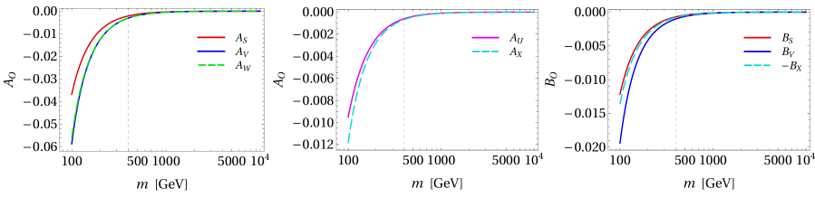
Figure 1: The coefficients $A_{O}$ and $B_{O}$ as functions of $m$ according to Eqs. (52) and (53). The dashed vertical line indicates the benchmark point value $m=400$ GeV.

Notice that, in general, the OPs $V$, $W$, and $X$ may be as important as $S$ and $U$.

This New Physics Model gives a fit of the OPs which is just a little worse than letting the OPs vary freely. Indeed, by setting $V=W=X=0$ and allowing $S$, $T$, and $U$ to vary freely we were able to accomplish a fit of all the relevant electroweak observables with $\chi^{2}=14.201$; while in our NPM with $m=400$ GeV, $n=5$, and $Y=3.3$ we achieve $\chi^{2}=14.894$, which is not much worse. We use the above values of $m$, $n$, and $Y$ as our first benchmark point (BP1). Then,

• Keeping both $n$ and $m$ fixed at their BP1 values, we let $Y$ vary and observe the variation of the OPs displayed in Fig. 2.

• Keeping both $n$ and $Y$ fixed at their BP1 values, we let $m$ vary and observe the variation of the OPs displayed in Fig. 3.

• Keeping both $Y$ and $m$ fixed at their BP1 values, we let $n$ vary and observe the variation of the OPs displayed in Fig. 4.

We also observe that there are approximate linear correlations between the parameters $S$ and $V$, and between the parameters $U$ and $X$, displayed in Fig. 5.

A more detailed description of the numerical analyses is given in subsection 6.4.

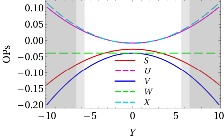
Figure 2: The oblique parameters as functions of $Y$, while $n=5$ and $m=400$ GeV are kept fixed. The dashed vertical line indicates the benchmark value $Y=3.3$. The light-gray area indicates that the corresponding OPs lead to a fit to the observables with $\chi^{2}>17$; for the dark-grey area one has $\chi^{2}>20$.

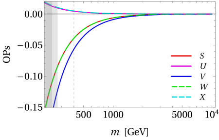
Figure 3: The oblique parameters as functions of $m$, while $n=5$ and $Y=3.3$ are kept fixed. The dashed vertical line indicates the benchmark value $m=400$ GeV. The meaning of the gray-shadowed bands is the same as in Fig. 2.

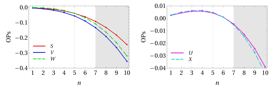
Figure 4: The oblique parameters as functions of $n$, while $m=400$ GeV and $Y=3.3$ are kept fixed. The dashed vertical line indicates the benchmark value $n=5$. The dark-gray area means that the OPs lead to $\chi^{2}>20$ fit.

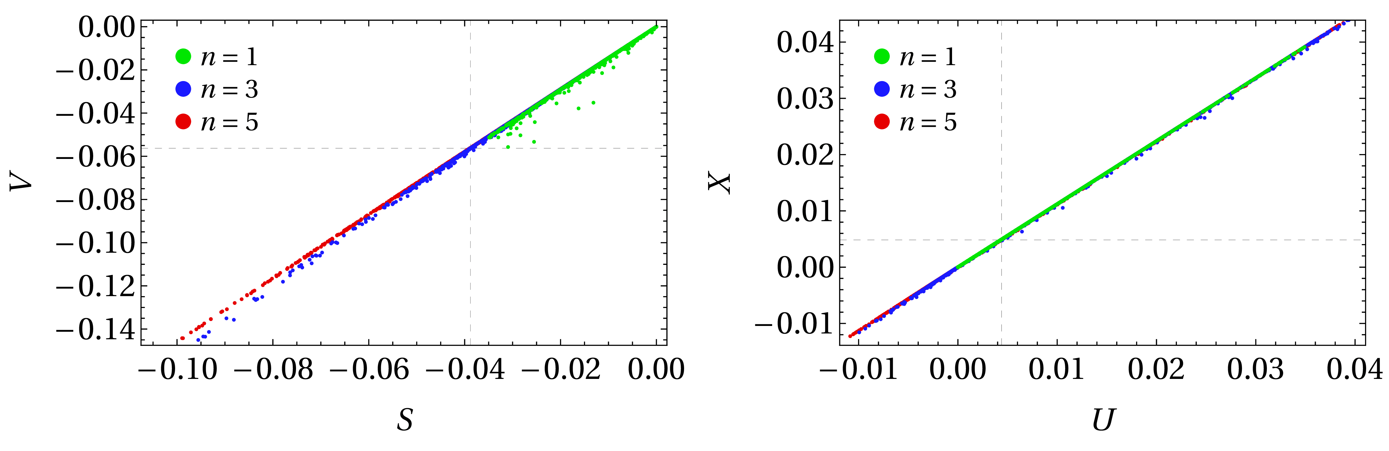
Figure 5: Correlation plots between oblique parameters for different values of $n$. The parameters $S$ and $V$ are distributed according to $V\approx 1.47\,S$ (left panel), while the parameters $U$ and $X$ obey $X\approx 1.12\,U$ (right panel). All points in the plots obey the restriction $\chi^{2}\leq 20$. The dashed lines indicate the values of the oblique parameters at the benchmark point BP1.

6 Two vector-like multiplets

Since the formalism in section 3 may look a bit abstract, we give in this section the practical calculation of the mixing matrices in a specific NPM with vector-like (in order to avoid anomalies) fermions. In our model all the fermion masses are justified either through bare mass terms or through $SU(2)\times U(1)$-invariant Yukawa couplings to the Higgs doublet of the SM; therefore, the oblique parameter $T$ has no reason to feature an UV divergence and, indeed, it converges.

6.1 Description of the model

In the NPM that we suggest there are, besides all the fermion multiplets and scalar multiplets of the SM, the following multiplets of fermions:

• One multiplet $A_{L}$ of left-handed fermions with isospin $J$ and hypercharge $Y$.

• One multiplet $B_{L}$ of left-handed fermions with isospin $J+1/2$ and hypercharge $Y+1/2$.

• Two multiplets $A_{R}$ and $B_{R}$ of right-handed fermions with the same quantum numbers as those of $A_{L}$ and $B_{L}$, respectively.

We define $n\equiv 2J+1$. Let the index $k$ run from $1$ to $n$, the index $j$ from $0$ to $n$, and the index $m$ from $1$ to $n-1$. We write the multiplets of additional fermions as

$$A_{E}=\left(\begin{array}[]{c}a_{1,E}\\ a_{2,E}\\ \vdots\\ a_{n,E}\end{array}\right),\quad B_{E}=\left(\begin{array}[]{c}b_{0,E}\\ b_{1,E}\\ b_{2,E}\\ \vdots\\ b_{n,E}\end{array}\right).$$ (54)

There are bare-mass terms given by

$$\mathcal{L}_{\mathrm{bare}}=-m_{A}\sum_{k=1}^{n}\,\overline{a_{k,R}}\ a_{k,L}-m_{B}\sum_{j=0}^{n}\,\overline{b_{j,R}}\ b_{j,L}+\mathrm{H.c.}$$ (55)

The quantum numbers of the new fermion multiplets were chosen in such a way that they have $SU(2)\times U(1)$-invariant Yukawa couplings to the Higgs doublet of the SM $\left(\varphi^{+},\ \varphi^{0}\right)^{T}$, which has isospin and hypercharge $1/2$. It is easy to convince oneself that the Yukawa couplings of $\varphi^{0}$ to the new fermions are given by

$$\mathcal{L}_{\mathrm{Yukawa}}=\cdots-\varphi^{0}\ \sum_{k=1}^{n}\sqrt{k}\,\left(y_{R}\ \overline{b_{k,R}}\ a_{k,L}+y_{L}\ \overline{b_{k,L}}\ a_{k,R}\right)+\mathrm{H.c.},$$ (56)

with Yukawa coupling constants $y_{R}$ and $y_{L}$. Since the largest Yukawa couplings are $y_{E}\sqrt{n}$, we assume that

$$\left|y_{R}\right|,\left|y_{L}\right|<\frac{4\pi}{\sqrt{n}}$$ (57)

in order to respect unitarity.

In Eq. (56), note that $b_{0,L}$ and $b_{0,R}$ have no Yukawa couplings to $\varphi^{0}$. Together they form a Dirac fermion with electric charge $\left.\left(n+1\right)\right/2+Y$. Its mass term is

$$-m_{B}\ \overline{b_{0,R}}\ b_{0,L}+\mathrm{H.c.}$$ (58)

For $k=1,\ldots,n$, there are two Dirac fermions with eletric charge $\left.\left(n+1\right)\right/2+Y-k$. According to Eqs. (55) and (56), their mass terms are given by

$$-\left(\begin{array}[]{cc}\overline{b_{k,R}},&\overline{a_{k,R}}\end{array}\right)\left(\begin{array}[]{cc}m_{B}&\sqrt{k}\,m_{C}\\ \sqrt{k}\,m_{D}&m_{A}\end{array}\right)\left(\begin{array}[]{c}b_{k,L}\\ a_{k,L}\end{array}\right).$$ (59)

In Eq. (59), $m_{C}\equiv y_{R}v$ and $m_{D}\equiv y_{L}^{\ast}v^{\ast}$, where $v$ is the VEV of $\varphi^{0}$, with $\left|v\right|\approx 174$ GeV. According to Eq. (57),

$$\left|m_{C}\right| < \frac{4\pi\left|v\right|}{\sqrt{n}},$$ (60a)

$$\left|m_{D}\right| < \frac{4\pi\left|v\right|}{\sqrt{n}},$$ (60b)

while $\left|m_{A}\right|$ and $\left|m_{B}\right|$ may be as large as one wishes. Our NPM has six real free parameters: $a\equiv\left|m_{A}\right|^{2}$, $b\equiv\left|m_{B}\right|^{2}$, $c\equiv\left|m_{C}\right|^{2}$, $d\equiv\left|m_{D}\right|^{2}$, $\arg{\left(m_{A}m_{B}m_{C}^{\ast}m_{D}^{\ast}\right)}$, and $Y$. Additionally there is $n$, which is an integer.

We diagonalize the mass matrix in Eq. (59) by making

$$\left(\begin{array}[]{c}b_{k,E}\\ a_{k,E}\end{array}\right)=\mathcal{U}_{k,E}\left(\begin{array}[]{c}f_{k,E}\\ g_{k,E}\end{array}\right),$$ (61)

where the $2\times 2$ matrices $\mathcal{U}_{k,E}$ are unitary and the physical fermions $f_{k}$ and $g_{k}$ have masses $m_{f,k}$ and $m_{g,k}$, respectively. We define

$$M_{k}=\left(\begin{array}[]{cc}m_{f,k}&0\\ 0&m_{g,k}\end{array}\right).$$ (62)

The matrices $M_{k}$ are diagonal and real. The bi-diagonalization condition is

$$\left(\begin{array}[]{cc}m_{B}&\sqrt{k}\,m_{C}\\ \sqrt{k}\,m_{D}&m_{A}\end{array}\right)=\mathcal{U}_{k,R}\,M_{k}\,\mathcal{U}_{k,L}^{\dagger}.$$ (63)

It is convenient to write

$$\mathcal{U}_{k,E}=\left(\begin{array}[]{c}X_{k,E}\\ Y_{k,E}\end{array}\right),$$ (64)

where $X_{k,E}$ and $Y_{k,E}$ are $1\times 2$ matrices. Thus, from Eq. (61),

$$b_{k,E} = X_{k,E}\left(\begin{array}[]{c}f_{k,E}\\ g_{k,E}\end{array}\right),$$ (65c)

$$a_{k,E} = Y_{k,E}\left(\begin{array}[]{c}f_{k,E}\\ g_{k,E}\end{array}\right),$$ (65f)

$$\left(\begin{array}[]{c}f_{k,E}\\ g_{k,E}\end{array}\right) = X_{k,E}^{\dagger}b_{k,E}+Y_{k,E}^{\dagger}a_{k,E}.$$ (65i)

The unitarity of $\mathcal{U}_{k,E}$ implies

$$X_{k,E}^{\ast}X_{k,E}^{T} = 1,$$ (66a)

$$Y_{k,E}^{\ast}Y_{k,E}^{T} = 1,$$ (66b)

$$X_{k,E}^{\ast}Y_{k,E}^{T}=Y_{k,E}^{\ast}X_{k,E}^{T} = 0,$$ (66c)

$$X_{k,E}^{T}X_{k,E}^{\ast}+Y_{k,E}^{T}Y_{k,E}^{\ast} = \mathbf{1}_{2},$$ (66d)

where $\mathbf{1}_{2}$ is the $2\times 2$ unit matrix. From Eqs. (63) and (64),

$$m_{B} = X_{k,R}\,M_{k}\,X_{k,L}^{\dagger},$$ (67a)

$$m_{A} = Y_{k,R}\,M_{k}\,Y_{k,L}^{\dagger},$$ (67b)

$$\sqrt{k}\,m_{C} = X_{k,R}\,M_{k}\,Y_{k,L}^{\dagger},$$ (67c)

$$\sqrt{k}\,m_{D} = Y_{k,R}\,M_{k}\,X_{k,L}^{\dagger}.$$ (67d)

Utilizing Eq. (66d) and remembering that $M_{k}=M_{k}^{\dagger}$, one may derive from Eqs. (67) that

$$b+kc = X_{k,R}\,M_{k}^{2}\,X_{k,R}^{\dagger},$$ (68a)

$$a+kd = Y_{k,R}\,M_{k}^{2}\,Y_{k,R}^{\dagger},$$ (68b)

$$b+kd = X_{k,L}\,M_{k}^{2}\,X_{k,L}^{\dagger},$$ (68c)

$$a+kc = Y_{k,L}\,M_{k}^{2}\,Y_{k,L}^{\dagger},$$ (68d)

6.2 The mixing matrices

We now apply our formalism to the model described in the previous subsection. Firstly, we put together all the physical fermions of each chirality in column vectors

$$V_{E}=\left(\begin{array}[]{c}b_{0,E}\\ f_{1,E}\\ g_{1,E}\\ \vdots\\ f_{n,E}\\ g_{n,E}\end{array}\right),$$ (69)

taking care to order the fermions by their decreasing electric charges. Indeed, the (diagonal) electric-charge matrix for the $2n+1$ physical fermions in $V_{E}$ is

$$Q=\frac{1}{2}\left(\begin{array}[]{cccccc}n+1&0_{1\times 2}&0_{1\times 2}&\cdots&0_{1\times 2}\\ 0_{2\times 1}&\left(n-1\right)\times\mathbf{1}_{2}&0_{2\times 2}&\cdots&0_{2\times 2}\\ 0_{2\times 1}&0_{2\times 2}&\left(n-3\right)\times\mathbf{1}_{2}&\cdots&0_{2\times 2}\\ \vdots&\vdots&\vdots&\ddots&\vdots\\ 0_{2\times 1}&0_{2\times 2}&0_{2\times 2}&\cdots&\left(1-n\right)\times\mathbf{1}_{2}\end{array}\right)+Y\times\mathbf{1}_{2n+1}.$$ (70)

The (diagonal) mass matrix of the physical fermions in $V_{E}$ is

$$M=\left(\begin{array}[]{ccccc}m_{B}&0_{1\times 2}&0_{1\times 2}&\ldots&0_{1\times 2}\\ 0_{2\times 1}&M_{1}&0_{2\times 2}&\ldots&0_{2\times 2}\\ 0_{2\times 1}&0_{2\times 2}&M_{2}&\ldots&0_{2\times 2}\\ \vdots&\vdots&\vdots&\ddots&\vdots\\ 0_{2\times 1}&0_{2\times 2}&0_{2\times 2}&\cdots&M_{n}\end{array}\right),$$ (71)

where the matrices $M_{k}$ have been defined in Eq. (62).

We define the matrices $M_{E}\left/\sqrt{2}\right.$, which represent the action of the $SU(2)$ operator $T_{+}$ on the fermions of $V_{E}$, through

$$V_{E}^{T}\,\frac{M_{E}}{\sqrt{2}}=\left(\begin{array}[]{cccccc}\left(T_{+}b_{0,E}\right),&\left(T_{+}f_{1,E}\right),&\left(T_{+}g_{1,E}\right),&\ldots,&\left(T_{+}f_{n,E}\right),&\left(T_{+}g_{n,E}\right)\end{array}\right).$$ (72)

Obviously, $T_{+}b_{0,E}=0$. Now, utilizing Eqs. (65),

$$\sqrt{2}\,T_{+}\left(\begin{array}[]{c}f_{1,E}\\ g_{1,E}\end{array}\right) = \sqrt{2}\,T_{+}\left(X_{1,E}^{\dagger}b_{1,E}+Y_{1,E}^{\dagger}a_{1,E}\right)$$ (73c)

$$= X_{1,E}^{\dagger}\,\sqrt{n}\ b_{0,E},$$ (73d)

and, for $m=1,\ldots,n-1$,

$$\sqrt{2}\,T_{+}\left(\begin{array}[]{c}f_{m+1,E}\\ g_{m+1,E}\end{array}\right) = \sqrt{2}\,T_{+}\left(X_{m+1,E}^{\dagger}b_{m+1,E}+Y_{m+1,E}^{\dagger}a_{m+1,E}\right)$$ (74c)

$$= \sqrt{n-m}\,\left(X_{m+1,E}^{\dagger}\sqrt{m+1}\,b_{m,E}+Y_{m+1,E}^{\dagger}\sqrt{m}\,a_{m,E}\right)$$ (74d)

$$= \sqrt{n-m}\left(\sqrt{m+1}\ X_{m+1,E}^{\dagger}X_{m,E}+\sqrt{m}\ Y_{m+1,E}^{\dagger}Y_{m,E}\right)\left(\begin{array}[]{c}f_{m,E}\\ g_{m,E}\end{array}\right).\hskip 22.76219pt$$ (74g)

Therefore,

$$M_{E}=\left(\begin{array}[]{cccccc}0&M_{E,0}&0_{1\times 2}&0_{1\times 2}&\cdots&0_{1\times 2}\\ 0_{2\times 1}&0_{2\times 2}&M_{E,1}&0_{2\times 2}&\cdots&0_{2\times 2}\\ 0_{2\times 1}&0_{2\times 2}&0_{2\times 2}&M_{E,2}&\cdots&0_{2\times 2}\\ \vdots&\vdots&\vdots&\vdots&\ddots&\vdots\\ 0_{2\times 1}&0_{2\times 2}&0_{2\times 2}&0_{2\times 2}&\cdots&M_{E,n-1}\\ 0_{2\times 1}&0_{2\times 2}&0_{2\times 2}&0_{2\times 2}&\cdots&0_{2\times 2}\end{array}\right),$$ (75)

where, from Eq. (73),

$$M_{E,0}=\sqrt{n}\,X_{1,E}^{\ast}$$ (76)

is a $1\times 2$ matrix, and the

$$M_{E,m}=\sqrt{n-m}\left(\sqrt{m+1}\ X_{m,E}^{T}X_{m+1,E}^{\ast}+\sqrt{m}\ Y_{m,E}^{T}Y_{m+1,E}^{\ast}\right)$$ (77)

are $2\times 2$ matrices. Notice that $M_{E}$ in Eq. (75), just like $Q$ in Eq. (70) and $M$ in Eq. (71), is a $\left(2n+1\right)\times\left(2n+1\right)$ matrix, because there are $2n+1$ (new) Dirac fermions in our NPM.

Let us now define the $2\times 2$ Hermitian, idempotent matrices

$$H_{k,E} \equiv X_{k,E}^{T}X_{k,E}^{\ast},$$ (78a)

$$\left(H_{k,E}\right)^{2} = H_{k,E}.$$ (78b)

(Equation (78b) follows from Eq. (66a).) It is then easy to see that

$$M_{E}M_{E}^{\dagger}=\left(\begin{array}[]{cccccc}M_{E,0}M_{E,0}^{\dagger}&0_{1\times 2}&0_{1\times 2}&\cdots&0_{1\times 2}&0_{1\times 2}\\ 0_{2\times 1}&M_{E,1}M_{E,1}^{\dagger}&0_{2\times 2}&\cdots&0_{2\times 2}&0_{2\times 2}\\ 0_{2\times 1}&0_{2\times 2}&M_{E,2}M_{E,2}^{\dagger}&\cdots&0_{2\times 2}&0_{2\times 2}\\ \vdots&\vdots&\vdots&\ddots&\vdots&\vdots\\ 0_{2\times 1}&0_{2\times 2}&0_{2\times 2}&\cdots&M_{E,n-1}M_{E,n-1}^{\dagger}&0_{2\times 2}\\ 0_{2\times 1}&0_{2\times 2}&0_{2\times 2}&\cdots&0_{2\times 2}&0_{2\times 2}\end{array}\right)$$ (79)

has, because of Eqs. (66),

$$M_{E,0}M_{E,0}^{\dagger} = n,$$ (80a)

$$M_{E,m}M_{E,m}^{\dagger} = \left(n-m\right)\left(m\times\mathbf{1}_{2}+H_{m,E}\right);$$ (80b)

while

$$M_{E}^{\dagger}M_{E}=\left(\begin{array}[]{cccccc}0&0_{1\times 2}&0_{1\times 2}&\cdots&0_{1\times 2}&0_{1\times 2}\\ 0_{2\times 1}&M_{E,0}^{\dagger}M_{E,0}&0_{2\times 2}&\cdots&0_{2\times 2}&0_{2\times 2}\\ 0_{2\times 1}&0_{2\times 2}&M_{E,1}^{\dagger}M_{E,1}&\cdots&0_{2\times 2}&0_{2\times 2}\\ \vdots&\vdots&\vdots&\ddots&\vdots&\vdots\\ 0_{2\times 1}&0_{2\times 2}&0_{2\times 2}&\cdots&M_{E,n-2}^{\dagger}M_{E,n-2}&0_{2\times 2}\\ 0_{2\times 1}&0_{2\times 2}&0_{2\times 2}&\cdots&0_{2\times 2}&M_{E,n-1}^{\dagger}M_{E,n-1}\end{array}\right)$$ (81)

has

$$M_{E,0}^{\dagger}M_{E,0} = n\times H_{1,E},$$ (82a)

$$M_{E,m}^{\dagger}M_{E,m} = \left(n-m\right)\left(m\times\mathbf{1}_{2}+H_{m+1,E}\right).$$ (82b)

Then, according to the definition (12),

$$H_{E}=M_{E}M_{E}^{\dagger}-M_{E}^{\dagger}M_{E}=\left(\begin{array}[]{ccccc}H_{E,0}&0_{1\times 2}&0_{1\times 2}&\cdots&0_{1\times 2}\\ 0_{2\times 1}&H_{E,1}&0_{2\times 2}&\cdots&0_{2\times 2}\\ 0_{2\times 1}&0_{2\times 2}&H_{E,2}&\cdots&0_{2\times 2}\\ \vdots&\vdots&\vdots&\ddots&\cdots\\ 0_{2\times 1}&0_{2\times 2}&0_{2\times 2}&\cdots&H_{E,n}\end{array}\right),$$ (83)

where

$$H_{E,0} = n,$$ (84a)

$$H_{E,k} = \left(n+1-2k\right)\times\mathbf{1}_{2}-H_{k,E}.$$ (84b)

Finally, the $\left(2n+1\right)\times\left(2n+1\right)$ Hermitian matrices $F_{E}$ are given by Eqs. (22), (70), and (83).

6.3 The finiteness of $T$

For completeness, in this subsection we explicitly demonstrate that Eq. (46) holds in our NPM and that, therefore, the oblique parameter $T$ is finite in it.

One may define

$$x_{E}\equiv\left\{\begin{array}[]{ll}c&\Leftarrow\ E=R,\\ d&\Leftarrow\ E=L.\end{array}\right.$$ (85)

Then, from Eqs. (68a) and (68c),

$$\mathrm{tr}\left(H_{k,E}M_{k}^{2}\right)=b+kx_{E}.$$ (86)

Also, Eqs. (68a), (68b), and (66d) imply

$$\mathrm{tr}\left(M_{k}^{2}\right)=a+b+k\left(c+d\right).$$ (87)

It is then easy to derive that

$$\mathrm{tr}\left(M_{E}M_{E}^{\dagger}M^{2}\right) = nb+\sum_{m=1}^{n-1}\left(n-m\right)\left\{m\left[a+b+m\left(c+d\right)\right]+b+mx_{E}\right\},$$ (88a)

$$\mathrm{tr}\left(M_{E}^{\dagger}M_{E}M^{2}\right) = n\left(b+x_{E}\right)+\sum_{m=1}^{n-1}\left(n-m\right)$$ (88b)

$$\times\left\{m\left[a+b+\left(m+1\right)\left(c+d\right)\right]+b+\left(m+1\right)x_{E}\right\},$$

$$\mathrm{tr}\left(H_{E}^{2}M^{2}\right) = n^{2}b+\sum_{k=1}^{n}\left\{\left(n+1-2k\right)^{2}\left[a+b+k\left(c+d\right)\right]\right.$$ (88c)

$$\left.+\left(4k-2n-1\right)\left(b+kx_{E}\right)\right\}.$$

Performing the sums over $m$ by using

$$\sum_{m=1}^{n-1}\,1 = n-1,$$ (89a)

$$\sum_{m=1}^{n-1}\,m = \left(n-1\right)\,\frac{n}{2},$$ (89b)

$$\sum_{m=1}^{n-1}\,m^{2} = \left(n-1\right)\,\frac{n\left(2n-1\right)}{6},$$ (89c)

$$\sum_{m=1}^{n-1}\,m^{3} = \left(n-1\right)^{2}\,\frac{n^{2}}{4},$$ (89d)

one finds that

$$\mathrm{tr}\left[\left(M_{E}M_{E}^{\dagger}+M_{E}^{\dagger}M_{E}-H_{E}^{2}\right)M^{2}\right]=0$$ (90)

for both $E=L$ and $E=R$. Therefore, each of the two lines (46a) and (46b) separately vanishes.

One also finds that

$$\mathrm{tr}\left(H_{L}MH_{R}M\right) = bH_{L,0}H_{R,0}+\sum_{k=1}^{n}\mathrm{tr}\left(H_{L,k}M_{k}H_{R,k}M_{k}\right)$$ (91c)

$$= bn^{2}+\sum_{k=1}^{n}\left\{\left(n+1-2k\right)^{2}\mathrm{tr}\left(M_{k}^{2}\right)\right.$$

$$\left.-\left(n+1-2k\right)\mathrm{tr}\left[\left(H_{k,L}+H_{k,R}\right)M_{k}^{2}\right]+\mathrm{tr}\left(H_{k,L}M_{k}H_{k,R}M_{k}\right)\right\}\hskip 19.91692pt$$

$$= bn^{2}+\sum_{k=1}^{n}\left\{\left(n+1-2k\right)^{2}\left[a+b+k\left(c+d\right)\right]\right.$$

$$\left.-\left(n+1-2k\right)\left[2b+k\left(c+d\right)\right]+b\right\},$$

$$\mathrm{tr}\left(M_{L}MM_{R}^{\dagger}M\right) = m_{B}\left(M_{L,0}M_{1}M_{R,0}^{\dagger}\right)+\sum_{m=1}^{n-1}\mathrm{tr}\left(M_{L,m}M_{m+1}M_{R,m}^{\dagger}M_{m}\right)$$ (91d)

$$= m_{B}n\left(X_{1,L}^{\ast}M_{1}X_{1,R}^{T}\right)$$

$$+\sum_{m=1}^{n-1}\left(n-m\right)\mathrm{tr}\left[\vphantom{\sqrt{m\left(m+1\right)}}\left(m+1\right)X_{m,L}^{T}X_{m+1,L}^{\ast}M_{m+1}X_{m+1,R}^{T}X_{m,R}^{\ast}M_{m}\right.$$

$$+mY_{m,L}^{T}Y_{m+1,L}^{\ast}M_{m+1}Y_{m+1,R}^{T}Y_{m,R}^{\ast}M_{m}$$

$$+\sqrt{m\left(m+1\right)}\,X_{m,L}^{T}X_{m+1,L}^{\ast}M_{m+1}Y_{m+1,R}^{T}Y_{m,R}^{\ast}M_{m}$$

$$\left.+\sqrt{m\left(m+1\right)}\,Y_{m,L}^{T}Y_{m+1,L}^{\ast}M_{m+1}X_{m+1,R}^{T}X_{m,R}^{\ast}M_{m}\right]$$

$$= nb+\sum_{m=1}^{n-1}\left(n-m\right)\left[\left(m+1\right)b+ma+m\left(m+1\right)\left(c+d\right)\right].$$

Therefore, once again performing the sums over $m$,

$$\mathrm{tr}\left(2\,M_{L}MM_{R}^{\dagger}M-H_{L}MH_{R}M\right)=0$$ (92)

and line (46c) is zero. Thus, in our model each of the three lines of Eq. (46) is separately zero.

6.4 Numerical results

Our benchmark point 2 (BP2) has $\left|m_{A}\right|=\left|m_{B}\right|=2000$ GeV, $\left|m_{C}\right|=\left|m_{D}\right|=100$ GeV, $\arg{\left(m_{A}^{\ast}m_{B}^{\ast}m_{C}m_{D}\right)}=1.5$, $Y=3.3$, and $n=5$. This yields a fit to the twenty electroweak observables with $\chi^{2}=14.214$, which is comparable to our best fit with null $V$, $W$, and $X$.

In order to explore the entire parameter space, we consider various integer values of $n$, we let the masses vary from 50 GeV to 3000 GeV but subject to the constraints (60), we let $\arg{\left(m_{A}^{\ast}m_{B}^{\ast}m_{C}m_{D}\right)}$ vary from $0$ to $2\pi$, and we let $Y$ go from $-10$ to $+10$. We keep only the points that have $\chi^{2}$ smaller than a certain number, which may be either 30, 20, or 17. This differentiation of the points according to their $\chi^{2}$ coincides well with the correlation between the $S$ and $T$ parameters in the electroweak fit, displayed in Fig. 6. This figure also shows that our NPM can only produce positive values for the parameter $T$.

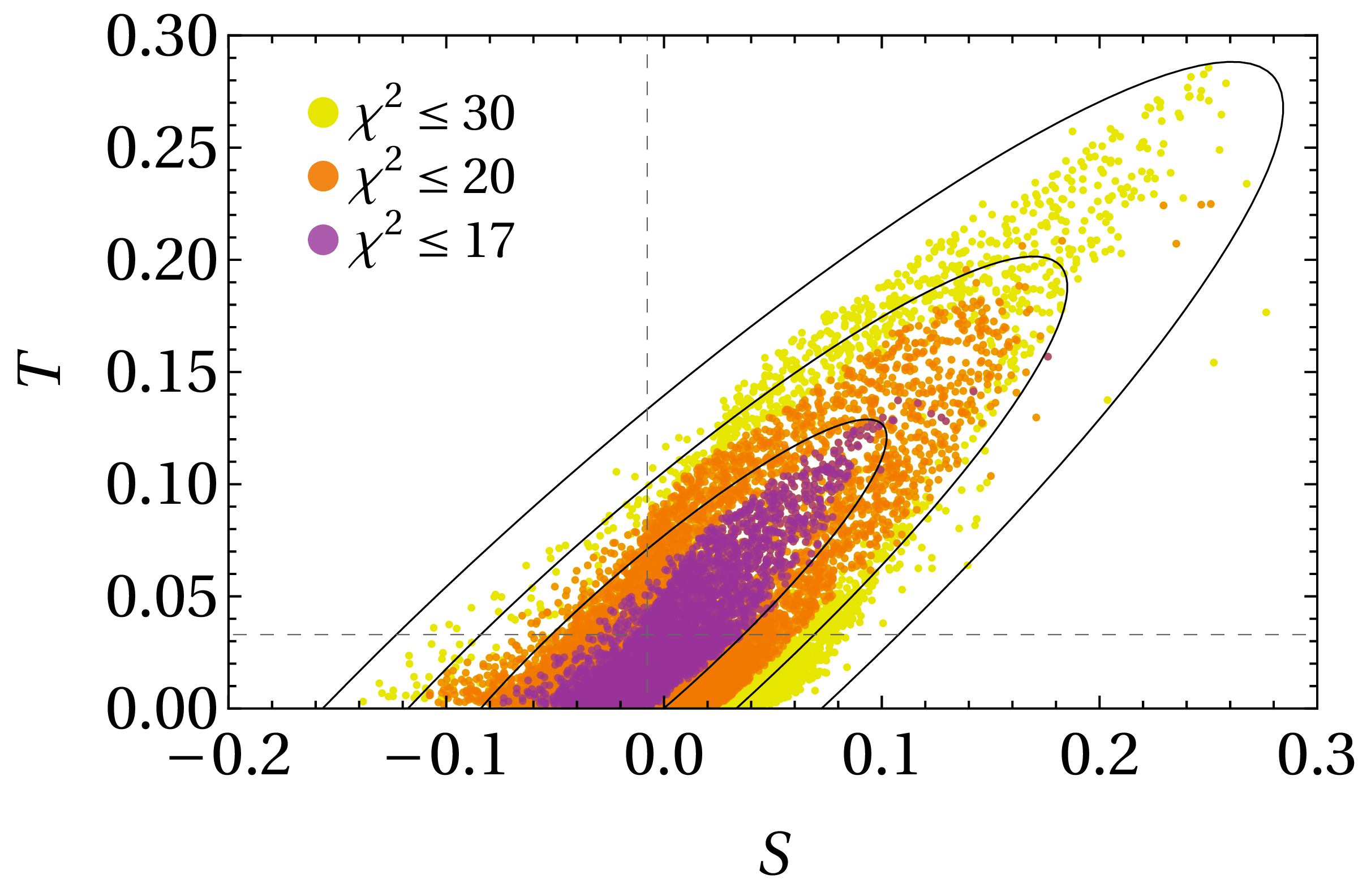
Figure 6: The correlation between the oblique parameters $S$ and $T$ in our New Physics Model, for $n=5$. The black ellipses correspond to the $1\sigma$, $2\sigma$, and $3\sigma$ (2dof) allowed regions in the $ST$ plane for a fit with $U=V=W=X=0$ and completely free $S$ and $T$. The dashed lines indicate the values of the oblique parameters at the benchmark point BP2.

In our NPM there is the approximate linear correlation between the oblique parameters $U$ and $X$ displayed in Fig. 7. The distribution of parameters is very similar to the one observed for the NPM of section 5, i.e. here too one has $X\approx 1.12\,U$.

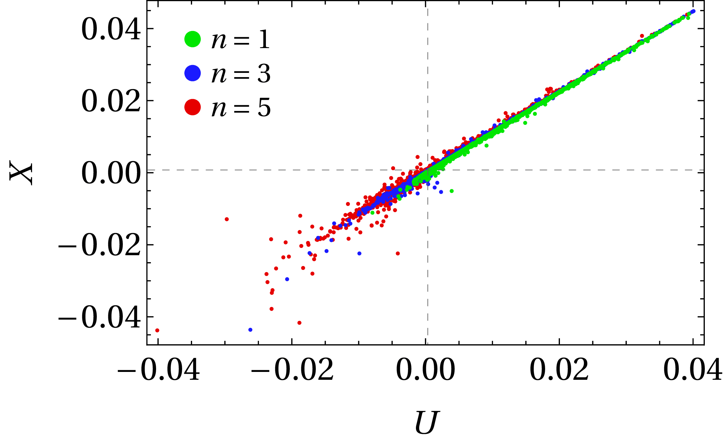
Figure 7: The correlation between the OPs $U$ and $X$, for different values of $n$. All the points in this plot have $\chi^{2}\leq 20$. The dashed lines indicate the values of the OPs in the BP2.

In Fig. 8 the variation of the OPs with $Y$ is displayed; all the other parameters of the model are kept fixed at their BP2 values. As ever, the OPs $W$ and $T$ are constant because Eqs. (28b) and (39), respectively, do not depend on $Y$. It should be noted that in this NPM the impact of $Y$ on $\chi^{2}$ is weak, contrary to what happened in the model of Section 5, cf. Fig. 2.

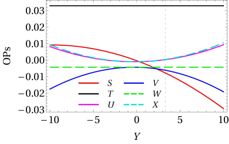
Figure 8: The OPs as functions of $Y$. The dashed vertical line indicates the BP2 value $Y=3.3$.

In Fig. 9 one observes that, as the value of $m_{A}=m_{B}$ increases, the absolute values of all the OPs decrease. Points with very low $m_{A}=m_{B}$ tend to have large $\chi^{2}$; $\chi^{2}\approx 14$ is minimal when $m_{A}=m_{B}=2000$ GeV (i.e., at the BP2), and increases up to $\approx 16$ for larger $m_{A}=m_{B}$.

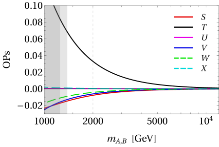
Figure 9: The OPs as functions of $m_{A}=m_{B}$. The dashed vertical line indicates the BP2 value $m_{A,B}=2000$ GeV. In the light-gray area, one obtains $\chi^{2}>17$; in the dark-gray area, $\chi^{2}>20$.

When we keep all the mass parameters and $Y$ fixed at their BP2 values, and we allow $n$ to vary, we observe the variation of the OPs displayed in Fig. 10. The absolute values of all the OPs increase with $n$ for $n>4$, and eventually $\chi^{2}$ becomes larger than at the BP2.

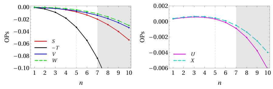
Figure 10: The OPs as functions of $n$. The dashed vertical line indicates the BP2 value $n=5$. The gray area corresponds to fits with $\chi^{2}>20$.

7 Conclusions

In this work we have presented general formulas for all six oblique parameters in an extension of the SM with additional fermions. The formulas are based on a formalism which defines matrices $M_{L}$ and $M_{R}$ that represent the action of the operator $T_{+}\left/\sqrt{2}\right.$ on the physical left- and right-handed fermions, respectively; here, $T_{+}$ is the raising operator of gauge-$SU(2)$. Starting from the matrices $M_{E}$ ($E=L,R$) one calculates the matrices $H_{E}\equiv\left[M_{E},M_{E}^{\dagger}\right]$ and then the matrices $F_{E}\equiv H_{E}-2Qs_{W}^{2}$, where $Q$ is the electric-charge matrix. The formulas for the OPs are then Equations (28), (31), (32), and (39), where one makes use of the functions $\mathcal{F}$, $\mathcal{G}$, and $\mathcal{H}$ defined in Eqs. (29), (33), and (40), respectively, and of functions defined in section 2.

We have applied our formulas to the cases of two models with new vector-like fermions in arbitrarily large representations of $SU(2)$. Remarkably, in both models we have found that the oblique parameters $V$ and $W$ are usually of the same order of magnitude as $S$, while the oblique parameters $X$ and $U$ tend to be somewhat smaller; however, these features may be upended when one is dealing with fermion representations featuring either a large isospin $J\gtrsim 2$ or a large hypercharge $\left|Y\right|\gtrsim 5$.

Acknowledgements:

L.L. thanks Heather Logan for pointing out to him Ref. [16]. The work of F.A. was supported by grant UI/BD/153763/2022. F.A. and L.L. were supported by the Portuguese Foundation for Science and Technology through projects UIDB/00777/2020, UIDP/00777/2020, and CERN/FIS-PAR/0002/2021; L.L. was furthermore supported by CERN/FIS-PAR/0019/2021. D.J. was supported by the Lithuanian Ministry of Education, Science and Sport through project CERN 2022-2027.

References

- [1] G. C. Branco, L. Lavoura, and J. P. Silva, “CP Violation.” Clarendon Press, Oxford, 1999.
- [2] I. Maksymyk, C. P. Burgess, and D. London, “Beyond , , and ,” Phys. Rev. D 50 (1994) 529.
- [3] See S. Draukšas, V. Dūdėnas, and L. Lavoura, “Oblique corrections when at tree level,” arxiv:2305.14050 [hep-ph], and the references therein.
- [4] F. Albergaria, L. Lavoura, and J. C. Romão, “Oblique corrections from triplet quarks,” J. High Energ. Phys. 03 (2023) 031.
- [5] F. Albergaria and L. Lavoura, “Oblique corrections from leptoquarks,” J. High Energ. Phys. 09 (2023) 080.
- [6] N. Bizot and M. Frigerio, “Fermionic extensions of the Standard Model in light of the Higgs couplings,” J. High Energ. Phys. 01 (2016) 036.
- [7] G. Passarino and M. J. G. Veltman, “One-loop corrections for annihilation into in the Weinberg model,” Nucl. Phys. B 160 (1979) 151.
- [8] T. Hahn, “Automatic loop calculations with FeynArts, FormCalc, and LoopTools,” Nucl. Phys. B Proc. Supp. 89 (2000) 231.
- [9] T. Hahn and M. Rauch, “News from FormCalc and LoopTools,” Nucl. Phys. B Proc. Supp. 157 (2006) 236.
- [10] L. Lavoura and J. P. Silva, “Oblique corrections from vectorlike singlet and doublet quarks,” Phys. Rev. D 47 (1993) 2046.
- [11] H.-H. Zhang, Y. Cao, and Q. Wang, “The effects on S, T and U from higher-dimensional fermion representations,” Mod. Phys. Lett. A 22 (2007) 2533.
- [12] Particle Data Group, R. L. Workman et al., “Review of Particle Physics”, Prog. Theor. Exp. Phys. 2022 (2022) 083C01.
- [13] S. Schael et al. [ALEPH, DELPHI, L3, OPAL, SLD, LEP Electroweak Working Group, SLD Electroweak Group, and SLD Heavy Flavour Group], “Precision electroweak measurements on the resonance,” Phys. Rept. 427 (2006) 257.
- [14] R. Tenchini, “Asymmetries at the Z pole: The Quark and Lepton Quantum Numbers,” Adv. Ser. Direct. High Energy Phys. 26 (2016) 161–184.
- [15] R. T. d’Agnolo, F. Nortier, G. Rigo, and P. Sesma, “The two scales of new physics in Higgs couplings,” J. High Energ. Phys. 08 (2023) 019.
- [16] D. Barducci, M. Nardecchia, and C. Toni, “Perturbative unitarity constraints on generic vector interactions,” J. High Energ. Phys. 09 (2023) 134.
- [17] K. Hally, H. E. Logan, and T. Pilkington, “Constraints on large scalar multiplets from perturbative unitarity,” Phys. Rev. D 85 (2012) 095017.