DeepSurveySim: Simulation Software and Benchmark Challenges for Astronomical Observation Scheduling

Abstract

Modern astronomical surveys have multiple competing scientific goals. Optimizing the observation schedule for these goals presents significant computational and theoretical challenges, and state-of-the-art methods rely on expensive human inspection of simulated telescope schedules. Automated methods, such as reinforcement learning, have recently been explored to accelerate scheduling. However, there do not yet exist benchmark data sets or user-friendly software frameworks for testing and comparing these methods. We present DeepSurveySim – a high-fidelity and flexible simulation tool for use in telescope scheduling. DeepSurveySim provides methods for tracking and approximating sky conditions for a set of observations from a user-supplied telescope configuration. We envision this tool being used to produce benchmark data sets and for evaluating the efficacy of ground-based telescope scheduling algorithms, particularly for machine learning algorithms that would suffer in efficacy if limited to real data for training. We introduce three example survey configurations and related code implementations as benchmark problems that can be simulated with DeepSurveySim.

1 Introduction

Modern astronomy experiments typically have multiple competing scientific goals. Each of these goals requires the observation of a different kind of astronomical object – e.g., static galaxies, time-varying stars (like supernovae), and transients (like planets). In an astronomical survey campaign that spans months to years, scheduling observations of objects typically requires competing scheduling priorities. For example, faint galaxies require multiple exposures of the same locations on the sky to reduce noise. Transients and variables, on the other hand require exposures at many different locations in the sky, which diverts telescope time away from the location for the galaxies. In addition, ground-based observing campaigns must contend with atmospheric conditions, which degrade data and can interrupt planned observations; weather conditions like clouds can interrupt a schedule or change the kinds of observations possible.  

Optimizing a schedule amidst these complex and competing observational goals typically necessitates a forward model (like a simulation) of the night sky, observing conditions, and telescope operations. These simulations are then used by a human to manually design a schedule or within optimization algorithms like Reinforcement Learning (RL). All methods still typically require human intervention, even if only to validate a schedule produced with an automated approach. However, the methods are not widely benchmarked or compared in detail, and a user-friendly, well-packaged, open-source simulation software to generate benchmark simulated data sets does not yet exist.

We present DeepSurveySim, an open-source software package for simulating ground-based surveys. We also present three standard challenge problems for the comparison of scheduling methods and algorithms. DeepSurveySim can be used to generate data sets for these benchmark challenges. These "challenge" benchmarks can be used for evaluating traditional scheduling methods. However, more importantly, they can supply easily accessible data generation tools for comparatively data-greedy Machine Learning algorithms.

This manuscript is organized as follows. In Section 2, we describe the current state of the art for simulators and open problems. In Section 3, we describe the simulator model. In Section 4, we present three challenge problems that can be used as benchmarks for scheduling algorithms.

2 Related Work

Individual experiments and surveys – like the Sloan Digital Sky Survey [18], the Dark Energy Survey [15], and the Rubin Observatory’s Legacy Survey of Space and Time (LSST) [10] – typically create codebases for internal usage only for generating simulations of schedules, developing scheduling algorithms, and assessing potential observing strategies. LSST conducted an open challenge within the collaboration for different research groups to create survey strategies optimized for their science [20] [6] [7] [11] [5] [16] [21].

Short survey campaigns can use tools like AstroPlan [11] for scheduling. However, campaigns for larger surveys require complex simulators and more automated methods. Some of the earliest work goes back to the Hubble Space Telescope’s work with SPIKE [8], which adapted factory automation planning techniques for ground-based telescopes. It was later applied for greedy search algorithms on moment-to-moment scheduling [17]. These methods were a step forward for automating scientific discovery, but largely inaccessible at the time due to the large amounts of computing and data required to use them, and their inability to adapt to interruptions. More advanced automated approaches employ adaptive scheduling[1], Reinforcement Learning (RL) algorithms [12, e.g.,], or semi-supervised graph neural networks [3, e.g.,]. All of these classes of techniques require an environment, in the real world or otherwise, to be trained. Training these algorithms on real-world data sets is infeasible because there isn’t enough historical data, and that historical data doesn’t provide enough information for future campaigns.

In any case, simulators and scheduling algorithms developed by surveys are rarely cross-compared or reported on in detail. In the development of DeepSurveySim, we draw inspiration from other tools for autonomous control in our design, such as the driving simulation, CARLA [4] and the flight system integration tool, OnAIR [9]. DeepSurveySim is based on simulation tools originally developed for DES and LSST [15].

3 DeepSurveySim: Simulator for ground-based optical telescopes

We introduce DeepSurveySim, a light-weight and high-fidelity open-source simulation software to aid in scheduling observations for astronomical survey campaigns. The simulator’s calculations are deterministic regarding the positions of sky objects and the telescope’s positions. Calculations are performed on-demand and do not require large amounts of storage space to save generated schedules and related parameters. The simulator is designed to be highly flexible, and it comes with simple predefined configurations for particular observing goals and conditions. The simulator is primarily designed for use in multiple settings with Markov chain policy-style algorithms. DeepSurveySim uses the Gymnasium API [19] as an inspiration for syntax. DeepSurveySimis specifically built to be used in conjunction with Gymnasium, allowing for integration with many different Machine Learning frameworks that support the package. There are two main sections – the ‘observation variables‘ and the ‘survey configuration‘ (Figure 1). This allows the simulation to calculate only the variables required for the policy algorithm to advance and decrease overall compute time, or to add more variables and metrics for diagnostic purposes. The user can designate the physical location of the observatory. It also allows for separation between the type of schedule being generated and the observatory it is designed for, which is useful for testing method generalization.

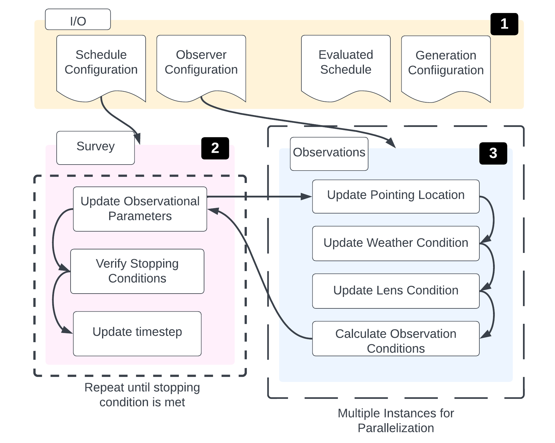
Figure 1: Workflow diagram for DeepSurveySim. The program initializes two different modules – the survey (2, pink) and the observation variables (3, blue) via a configuration files (1, yellow). The survey is then executed by calculating updated positions of sky locations and sky conditions until a user-defined stopping condition is met.

The simulator has the following key features:

Independent Configuration Files The simulator ingests configuration files, which are intended to be mixed and matched across varying observing scenarios (discussed in Section 4) and observatories. This allows for high levels of reproducibility.

Position Tracking The simulator tracks four variables of the telescope’s physical configuration: the Right Ascension, Declination, Filter Wavelength Band, and Time (in Modified Julian Date). These are specified by the user at each step or are ingested in bulk as an array. The tracking functionality includes the option to account for time regarding the slew (telescope-repositioning), change of filters, or to include a level of inaccuracy in the repositioning system of the telescope, dependent on the angular distance between two observations.

Condition Tracking The simulator uses the packages Astropy [2] and SkyBright [13] for condition calculation. The simulator’s calculation includes the position and brightness of the sun and moon relative to the telescope, approximated atmospheric conditions, and the position of the telescope relative to the earth. The full list of variables and their extended definitions can be found in Table 2 in the Appendix. These allow a policy to walk through any given initial conditions and calculate a representation of the sky at a particular point in time, which permits the evaluation of the effectiveness of the scheduling algorithm.

Approximate Weather Given reference sky conditions for an observatory, the DeepSurveySim selects approximate seeing and cloud conditions based on the time of year. It takes as input the mean cloud cover for that time of year – using reference weather station data supplied by a user, dependent on the location of their observatory – and applies a threshold to determine if seeing and cloud extinction would be impacted.

4 Benchmark Challenge Problems

We provide a set of problems with corresponding code implementations. However, we encourage using these problems as a template to construct more specific scenarios to simulate.

4.1 Problem 1: Maximizing Observation Quality in a Predetermined Set of Survey Fields

Maximizing observation quality is one of the simplest problems to consider. Addressing this challenge typically requires producing a ’greedy’ algorithm that can predict the next step that has the highest-quality observations, and produce the paired action for the telescope to move it to that site. We use the effective exposure time $\tau_{eff}$ defined as a simple proxy metric for ensuring the observation is high-quality and low-noise:

$$\tau_{eff}=(\eta*\frac{0.9}{\textsc{fwhm}})^{2}*\frac{b_{ref}}{b}*\tau_{exposure};$$ (1)

$\eta$ is the amount of light from a target reaching through the atmosphere as measured by instrumentation; fwhm is the blurring of an image resulting from instrumentation and atmospheric conditions; $\frac{b_{ref}}{b}$ is the magnitude of the sky brightness measured against a reference moonless night; and $\tau_{exposure}$ is the exposure time of a given observation. Further explanation can be found in [14].

This problem lacks realism because surveys generally have much more specific and complicated goals. Nevertheless, this example can be useful for validation of a given method. This can be done by selected a small subset of sites (such as a small cluster along the equator), and verifying the method created the observation schedule for this site that provides the maximum schedule quality according to Equation 2.

A schedule that aims to maximize observation clarity for all images can be evaluated directly. The quality ($R$) of schedule $s_{n}$ over the discrete time interval $T=[t_{0},t_{final}]$, where $t_{0}$ is the starting time of the schedule and $t_{final}$ is the end, is given by: $R_{s_{n}}=\frac{1}{||T||}\Sigma^{t_{n}}_{t=0}\tau_{eff_{t}}$.

Consider the scenario in which there is a finite number of pre-designated observation sites ($S$) and in which the observation schedule is created on the fly. Then, the overall survey quality can be measured with

$$R_{s_{n}}=\frac{1}{||T||}\frac{\Sigma^{t_{n}}_{t=0}\tau_{eff_{t}}(s_{selected_{t}})}{\Sigma^{t_{n}}_{t=0}max\{\tau_{eff_{t}}(s_{t}):s\in S\}}.$$ (2)

where $s_{selected_{t}}$ is the site selected for the observation at time $t$.

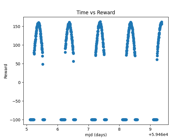
(a)

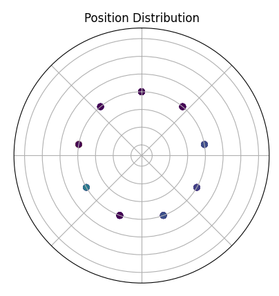
(b)

Figure 3: An example solution to the problem described in 4.1, using a Reinforcement Learning algorithm limited to an equatorial survey ($decl=0$). (a) The values of Equation  1 across multiple nights. The negative values are associated with a negative "penalty" term applied to steps that are outside the user defined allowed range of $\tau_{eff}$. This occurs at dawn and dusk when the sky brightness has dramatically increased. (b) The location of the selected observations projected onto a polar map where the angular distance from vertical ($ra=0$) represents Right Ascension. The lighter colors on sites chosen by the algorithm represents relatively higher reward.

This means that each step of the scheduling algorithm only requires the current state to make a decision about the next observation. This produces a schedule that can be stopped and started to account either for unscheduled downtime. We provide an example of a schedule created with this evaluation metric in Figure 3 in the Appendix.

4.2 Problem 2: Maximizing Observations of an Object with Low Visibility

In some cases, there are objects of interest that are rarely visible – e.g., transients that are in motion (like comets) or statistically rare events (like supernovae). Transients have a deterministic trajectory, the observation of which can be explicitly accounted for in the environment as a rule for the schedule design: at time $t$, the action is always $a$ without being allowed to deviate. The remainder of the schedule is planned around this constraint. Rare events require deviations from the preset schedule to account for the chance of observing something in a given field. One of the major challenges in this scenario is enabling the schedule to recover from the observation of the stochastic event. This logic can also be applied in the case where weather events cause a stochastic variation in observability of a given part of the sky. This presents an opportunity for the scheduling problem to be treated as a multi-objective optimization problem, which is represented by:

$$R_{s_{n}}=\frac{1}{||T||}(||\{s_{i}:s_{i}\in S_{interest}\}||+\lambda\Sigma^{t_{n}}_{t=0}\tau_{eff_{t}}(s_{t})),$$ (3)

where $S_{interest}$ denotes the condition of the observation containing the desired object, and $\lambda$ is a user-defined hyperparameter that determines the weight of observations $s\notin S_{interest}$.

4.3 Problem 3: Maximize Uniformity of Image Quality Across Sites

Amongst the three example problems presented in this work, this problem is the most generic and has the widest application. A typical observing goal is uniformity of image quality $\theta$ across the survey. This can be defined numerically as:

$$R_{S_{n}}=\frac{1}{||T||*Var(\{\tau_{eff}(s_{i}):s_{i}\in S_{n})\}}*\Sigma^{t_{n}}_{i=0}\begin{cases}\tau_{eff}(s_{i})&\tau_{eff}(s_{i})\geq\theta\\ 0&\tau_{eff}(s_{i})<\theta\\ \end{cases}.$$ (4)

We must also prevent the algorithm from "cheating" and selecting only one location. In our formulation, we determine that the schedule should be assigned a quality of 0 if it does not capture all sites at least $N$ times.

5 Conclusions

Scheduling is not an easy task, and telescope scheduling, with all its possible stochastic interruptions, is even less so. We hope the introduction of a standardized simulation tool DeepSurveySim will make the evaluation of novel approaches more viable.

Limitations This project is limited to deterministic variables, so random events in either atmosphere conditions or rare cosmological events are not modeled. The approximations of atmospheric conditions used by the simulation only holds for altitudes $\geq 20^{\circ}$ so observations very close to the horizon are inaccurate. Included weather condition calculations are based on historical measurements, so will not capture changes in the environmental trends.

Appendix

Table 1: Glossary of terms and associated symbols used throughout this paper, in order of appearance. These are supplied for reference and ease of reading.

Name	Symbol	Definition
Schedule	–	Sequence of observations ordered by time
Survey	–	Collection of observations, unordered
Zenith Angle	$\phi$	90∘ tangential to the Earth’s surface
Markov Decision Process	MDP	Decision making process that takes the current state, increments it using a pre-defined policy, and calculates the benefit of this new state
Reinforcement Learning	RL	MDP Based learning schema where a optimization algorithm learns the policy used to increment the state
Right Ascension	RA	Angular distance east or west of the point in the celestial equator where the sun is centered during the Spring equinox
Declination	Decl.	Angular distance north or south of the celestial equator
Modified Julian Date	MJD	Number of days since 17 November 1858
Site/Observation/Pointing	–	The location of a singular measurement from the telescope
Discrete Time Intervals	$T$	Collection of time steps a schedule covers
Possible Sites	$S$	Collection of observations included in a survey
Schedule Quality	$R_{s_{n}}$	The cumulative quality of all the observations in a schedule
–	$\lambda$	Weighting factor used to scale observations that are not in the target survey
Quality Threshold	$\theta$	Lower threshold on the designated quality to determine if an observation is within the standards required for the survey
Cardinality Threshold	$N$	Lower threshold on the number times a site must be measured during a survey

Table 2: All possible variables included in the simulation framework. At the discretion of the user, if a variable is not directly involved in the evaluation of the schedule $R$, the variable can be removed to increase the speed of calculations.

Name	Name in package	Description
Local Sidereal Time	lst	Time, in units of the local sidereal time
Transverse Seeing	pt_seeing	Blurring of the image due to optical distortion by the atmosphere
Band Seeing	band_seeing	Blurring of the image due to optical distortion by instrumentation
Seeing	fwhm	Combined impact of transverse and band seeing
Airmass	airmass	Line integral of air density along the angle the telescope is observing
Hour Angle	ha	Angular distance between the zenith and the site of interest
Moon Hour Angle	moon_ha	Angular distance between the zenith and the moon
Moon Elongation	moon_elongation	Position of the moon in its orbit around the earth
Moon Phase	moon_phase	Moon phase in a % of a full moon
Moon Separation	moon_separation	Angular distance between the target observation location and the moon
Moon Right Ascension	moon_ra	Right ascension of the moon’s position
Moon Declination	moon_decl	Declination of the moon’s position
Moon Airmass	moon_airmass	Airmass if the telescope was to directly observe the moon
Azimuthal Angle	az	Rotation of the telescope about its axis
Altitude	alt	Height of the apex of the telescope with respect to the ground
Hour Angle	ha	Angular distance between the zenith
Sun Hour Angle	sun_ha	Angular distance between the zenith and the sun
Sun Airmass	sun_airmass	Airmass if the telescope was to directly observe the sun
Sun Right Ascension	sun_ra	The right ascension of the sun’s position
Sun Declination	sun_decl	The declination of the sun’s position
Atmospheric transmission ($\eta$)	sky_magnitude	The fraction of light from astronomical sources that makes it through the atmosphere [14]
$\tau$	tau	Instantaneous measure of sky quality with respect to an observation
$\tau_{eff}$	teff	Measure of observation quality as defined in Equation 1

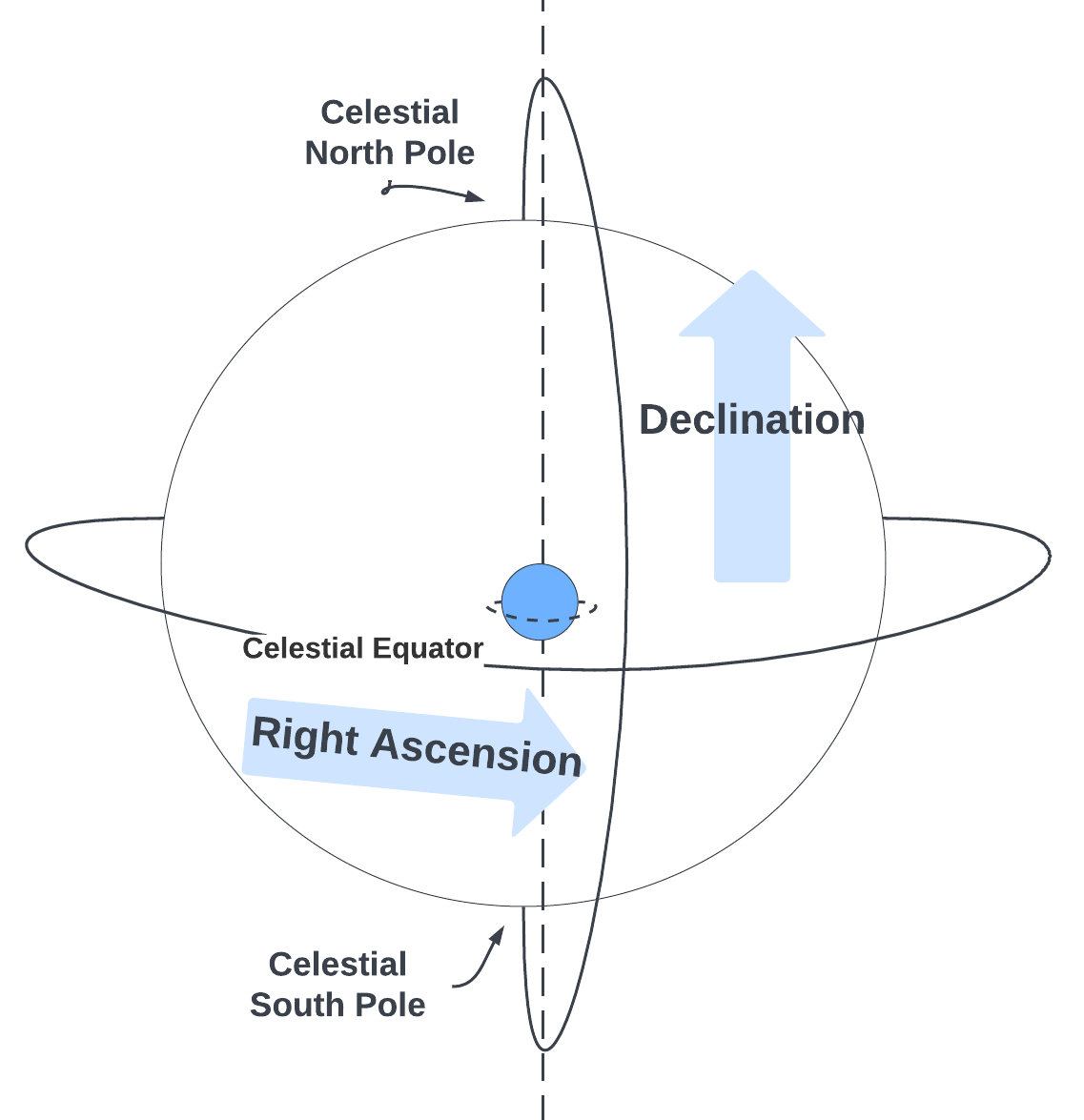
Figure 2: A simple map of the relationship between Right Ascension and Declination. Declination is the angle displaced vertically from the celestial equator, where positive declination denotes an observation in the northern sky, and negative declination denotes the southern sky. Right Ascension is the displacement from the point in the celestial equator where the sun is centered during the Spring equinox.

References

- [1] Adaptive Scheduler. Observatory Control System, August 2023.
- [2] Astropy Collaboration, Adrian M. Price-Whelan, Pey Lian Lim, Nicholas Earl, Nathaniel Starkman, Larry Bradley, David L. Shupe, Aarya A. Patil, Lia Corrales, C. E. Brasseur, Maximilian N"othe, Axel Donath, Erik Tollerud, Brett M. Morris, Adam Ginsburg, Eero Vaher, Benjamin A. Weaver, James Tocknell, and et. al. The Astropy Project: Sustaining and Growing a Community-oriented Open-source Project and the Latest Major Release (v5.0) of the Core Package. apj, 935(2):167, August 2022.
- [3] Miles Cranmer, Peter Melchior, and Brian Nord. Unsupervised Resource Allocation with Graph Neural Networks, June 2021. arXiv:2106.09761 [astro-ph].
- [4] Alexey Dosovitskiy, German Ros, Felipe Codevilla, Antonio Lopez, and Vladlen Koltun. CARLA: An open urban driving simulator. In Proceedings of the 1st Annual Conference on Robot Learning, pages 1–16, 2017.
- [5] R. J. Foley, A. M. Koekemoer, D. N. Spergel, F. B. Bianco, P. Capak, L. Dai, O. Dore, G. G. Fazio, H. Ferguson, A. V. Filippenko, B. Frye, L. Galbany, E. Gawiser, C. Gronwall, N. P. Hathi, C. Hirata, R. Hounsell, S. W. Jha, A. G. Kim, P. L. Kelly, J. W. Kruk, S. Malhotra, K. S. Mandel, R. Margutti, D. Marrone, K. B. W. McQuinn, P. Melchior, L. Moustakas, J. A. Newman, J. E. G. Peek, S. Perlmutter, J. D. Rhodes, B. Robertson, D. Rubin, D. Scolnic, R. Somerville, R. Street, Y. Wang, D. J. Whalen, R. A. Windhorst, and E. J. Wollack. LSST Observing Strategy White Paper: LSST Observations of WFIRST Deep Fields. arXiv e-prints, page arXiv:1812.00514, November 2018.
- [6] T. Grav, A. K. Mainzer, and T. Spahr. Modeling the Performance of the LSST in Surveying the Near-Earth Object Population. AJ, 151(6):172, June 2016.
- [7] Philippe Gris, Nicolas Regnault, Humna Awan, Isobel Hook, Saurabh W. Jha, Michelle Lochner, Bruno Sanchez, Dan Scolnic, Mark Sullivan, Peter Yoachim, and LSST Dark Energy Science Collaboration. Designing an Optimal LSST Deep Drilling Program for Cosmology with Type Ia Supernovae. APJS, 264(1):22, January 2023.
- [8] Mark Johnston. AUTOMATED TELESCOPE SCHEDULING. Symposium on Coordination of Observational Projects, 1987.
- [9] James et. al. Marshall. onair. https://github.com/nasa/OnAIR, 2023.
- [10] Phil Marshall, Will Clarkson, Ohad Shemmer, Rahul Biswas, Miguel De Val-Borro, Jeonghee Rho, Lynne Jones, Timo Anguita, Stephen Ridgway, Federica Bianco, Zeljko Ivezic, Michelle Lochner, Josh Meyers, Kathy Vivas, Melissa Graham, Chuck Claver, Seth Digel, Vishal Kasliwal, and Peregrine M McGehee et. al. Lsst science collaborations observing strategy white paper: "science-driven optimization of the lsst observing strategy", 2017.
- [11] Brett M. Morris, Erik Tollerud, Brigitta Sipőcz, Christoph Deil, Stephanie T. Douglas, Jazmin Berlanga Medina, Karl Vyhmeister, Toby R. Smith, Stuart Littlefair, Adrian M. Price-Whelan, Wilfred T. Gee, and Eric Jeschke. astroplan: An Open Source Observation Planning Package in Python. AJ, 155(3):128, March 2018.
- [12] Elahesadat Naghib, Peter Yoachim, Robert J. Vanderbei, Andrew J. Connolly, and R. Lynne Jones. A Framework for Telescope Schedulers: With Applications to the Large Synoptic Survey Telescope. AJ, 157(4):151, March 2019. arXiv:1810.04815 [astro-ph].
- [13] Eric Neilsen. skybright. 2 2019.
- [14] Eric H. Neilsen, Jr., James T. Annis, H. Thomas Diehl, Molly E. C. Swanson, Chris D’Andrea, Stephen Kent, and Alex Drlica-Wagner. Dark energy survey’s observation strategy, tactics, and exposure scheduler. 2019.
- [15] Jr. Neilsen, Eric H., James T. Annis, H. Thomas Diehl, Molly E. C. Swanson, Chris D’Andrea, Stephen Kent, and Alex Drlica-Wagner. Dark Energy Survey’s Observation Strategy, Tactics, and Exposure Scheduler. arXiv e-prints, page arXiv:1912.06254, December 2019.
- [16] Knut Olsen, Marcella Di Criscienzo, R. Lynne Jones, Megan E. Schwamb, Hsing Wen ”Edward” Lin, Humna Awan, Phil Marshall, Eric Gawiser, Adam Bolton, and Daniel Eisenstein. A Big Sky Approach to Cadence Diplomacy. arXiv e-prints, page arXiv:1812.02204, December 2018.
- [17] Roberto J. Samson. Greedy search algorithm used in the automated scheduling of Hubble Space Telescope activities. In Peter J. Quinn, editor, Observatory Operations to Optimize Scientific Return, volume 3349, pages 282 – 290. International Society for Optics and Photonics, SPIE, 1998.
- [18] Felipe A. Santana, Rachael L. Beaton, Kevin R. Covey, Julia E. O’Connell, Penélope Longa-Peña, Roger Cohen, José G. Fernández-Trincado, Christian R. Hayes, Gail Zasowski, Jennifer S. Sobeck, Steven R. Majewski, and S. D. Chojnowski et. al. Final targeting strategy for the sdss-iv apogee-2s survey. The Astronomical Journal, 162(6):303, dec 2021.
- [19] Mark Towers, Jordan K. Terry, Ariel Kwiatkowski, John U. Balis, Gianluca de Cola, Tristan Deleu, Manuel Goulão, Andreas Kallinteris, Arjun KG, Markus Krimmel, Rodrigo Perez-Vicente, Andrea Pierré, Sander Schulhoff, Jun Jet Tai, Andrew Tan Jin Shen, and Omar G. Younis. Gymnasium, March 2023.
- [20] A. S. Villarreal, Yadu Babuji, Tom Uram, Daniel S. Katz, Kyle Chard, and Katrin Heitmann. Extreme Scale Survey Simulation with Python Workflows. arXiv e-prints, page arXiv:2109.12060, September 2021.
- [21] Kathryn Volk, Megan E. Schwamb, Wes Fraser, Michael S. P. Kelley, Hsing Wen, Lin, Darin Ragozzine, R. Lynne Jones, Colin Snodgrass, and Michele T. Bannister. The Effects of Filter Choice on Outer Solar System Science with LSST. arXiv e-prints, page arXiv:1812.00937, December 2018.