Fast Explicit Solutions for Neutrino-Electron Scattering: Explicit Asymptotic Methods

Abstract

We present results of explicit asymptotic approximations applied to neutrino–electron scattering in a representative model of neutrino population evolution under conditions characteristic of core-collapse supernova explosions or binary neutron star mergers. It is shown that this approach provides stable solutions of these stiff systems of equations, with accuracy and timestepping comparable to that for standard implicit treatments such as backward Euler, fixed point iteration, and Anderson-accelerated fixed point iteration. Because each timestep can be computed more rapidly with the explicit asymptotic approximation than with implicit methods, this suggests that algebraically stabilized explicit integration methods could be used to compute neutrino evolution coupled to hydrodynamics more efficiently in stellar explosions and mergers than the methods currently in use.

I Introduction

Computer simulations of events like core collapse supernova explosions or neutron star mergers require solving simultaneously coupled systems of non-linear partial differential equations governing hydrodynamics, neutrino radiation transport, and thermonuclear reactions. Because rate parameters entering into these processes can differ by many orders of magnitude, such systems are computationally stiff and stability demands that great care be taken in choosing methods to solve them Oran and Boris (2005); Gear (1971); Lambert (1991); Press et al. (1992). Explicit methods are generally easier to implement than implicit ones because they require only the current state of the system to compute a future state, whereas implicit methods require also information at the next step, which is initially unknown so an iterative procedure is necessary. This iteration often involves matrix inversions at each step that are increasingly expensive for larger sets of equations. Thus computing an explicit timestep is generally faster and less memory intensive than computing an implicit timestep for large networks because they do not require matrix inversions. However traditional explicit methods such as forward Euler are impractical for solving the extremely stiff systems characteristic of many astrophysical processes because maintaining stability restricts the integration timesteps to tiny values, and this far outweighs the faster explicit computation of each timestep.

Thus standard explicit methods have usually been thought impractical for stiff systems, forcing the use of stable but more complex implicit methods. Because of the matrix inversions, these implicit methods are often prohibitively slow for networks of realistic size and complexity when coupled to a large-scale fluid dynamics simulation. This has typically forced the use of drastic approximations, often employing implicit networks that are stable but too small and/or too schematic to be realistic. We characterize such approximations as poorly controlled, as they introduce systematic errors that can be estimated only qualitatively because they are dictated by the ability to integrate the network with the chosen method rather than by the realistic physics of the network. But in a large-scale simulation of say a supernova, typically a multidimensional hydrodynamical code is coupled to kinetic networks (coupled ordinary differential equations) representing thermonuclear burning and/or neutrino evolution, and it may be argued that these kinetic networks need be solved only approximately, provided that the approximation introduces controlled errors that are smaller than the errors and uncertainties associated with the overall coupled hydrodynamical–kinetic system.

Given the current state of the art in such simulations, a conservative rule of thumb is that (controlled) errors of a few percent or less are acceptable for approximate kinetic networks, since to do better wastes resources and will not improve the final results. This raises the question of whether there exist approximations for standard explicit methods that could allow taking more competitive timesteps with an acceptable controlled error, thus permitting the solution of larger and more realistic kinetic networks coupled to fluid dynamics.

In a series of publications Guidry (2012); Guidry et al. (2013a); Guidry and Harris (2013); Guidry et al. (2013b); Feger (2011); Chupryna (2008); Brey (2022); Brock et al. (2015); Haidar et al. (2016); Guidry et al. (2023); Brey et al. (2023), our group has demonstrated a new class of algebraically stabilized explicit approximations for thermonuclear networks that extends earlier work by Mott and collaborators Mott et al. (2000); Mott (1999). These new explicit methods use algebraic constraints to stabilize explicit integration steps, resulting in stable timesteps that are comparable to those of standard implicit methods, even for extremely stiff systems of equations where the fastest and slowest rates can differ by 10-20 orders of magnitude. These methods require matrix–vector multiplication but not matrix inversions, so they scale more gently with network size than implicit algorithms. This more favorable scaling coupled with a competitive integration stepsize allowed a demonstration that such algorithms are capable of performing numerical solution of extremely stiff kinetic networks containing hundreds of species 5-10 times faster than standard implicit methods on a single CPU (Central Processing Unit) Guidry (2012); Guidry et al. (2013a); Guidry and Harris (2013); Guidry et al. (2013b). Furthermore, we found these explicit algebraic methods to be extremely amenable to GPU (Graphical Processing Unit) acceleration, permitting of order $1000$ large (150-isotope) thermonuclear networks to be executed in parallel on a single GPU in the time required for one such network to be solved by standard implicit means Brock et al. (2015); Haidar et al. (2016).

The demonstrations described above were for astrophysical thermonuclear networks but there is no fundamental reason why such methods cannot be applied to other stiff kinetic networks in many scientific applications, since most such networks have a mathematical and computational structure similar to that of thermonuclear networks Guidry (2012). To this end, we note that an adequate description of neutrino transport often is of fundamental importance for very high-temperature, very high density environments like those found in core collapse supernovae or binary neutron star mergers. Most large-scale simulations dealing with neutrinos have been forced to make significant approximations in the neutrino transport, and often in such simulations the largest fraction of the computing budget is allocated to evolution of neutrinos, even when they are treated approximately Mezzacappa et al. (2020); Foucart (2023). Accordingly, we have begun developing codes that apply explicit algebraic algorithms similar to those developed for thermonuclear networks to the evolution of neutrino populations.

Our suite of neutrino codes is being written primarily in C++ and will be referred to collectively as FENN (Fast Explicit Neutrino Network). It is our intention to make FENN available as a documented, open source, community resource. In this paper we present the first application of the new explicit algebraic methods implemented in FENN to evolution of neutrino populations due to neutrino-electron scattering (NES) under the hot, dense conditions characteristic of explosions and mergers. Mezzacappa & Bruenn Mezzacappa and Bruenn (1993) demonstrated the impact of a realistic treatment of NES, as opposed to more approximate Fokker–Plank treatments Myra et al. (1987), on the dynamics of stellar core collapse. Down-scattering mediated by NES increases the neutrino mean free path, which can result in increased deleptonization, and a reduced electron fraction in the collapsed core. See also Lentz et al. (2012a, b); Just et al. (2018) for further discussions on the role of NES and the complex interplay of neutrino opacities in supernova models. It is generally accepted that NES is part of the minimal set of opacities to include in realistic models Burrows et al. (2006); Janka (2012); Fischer et al. (2017); Mezzacappa et al. (2020).

Since NES couples neutrinos across momentum space, their inclusion in realistic models is computationally taxing and approximations have been employed to lessen the burden, including artificially reducing the scattering kernel to allow for explicit integration Thompson et al. (2003); O’Connor (2015); Just et al. (2018). Here we investigate the utility of approximating the NES operator to enable explicit integration with controlled errors. We shall find strong evidence that speedups relative to standard implicit methods similar to those found for thermonuclear networks hold also for neutrino networks, suggesting a viable path to faster solution of neutrino transport equations through algebraically stabilized explicit integration.

II Mathematical model of Neutrino-Electron Scattering

The basic problem is formulated as the evolution of a spectral neutrino number distribution discretized as a set of energy bins, each of phase-space volume $V$, with neutrino scattering into and out of the energy bins governed by the Boltzmann equation. For this particular model we use a Boltzmann equation that is spatially homogeneous, with inelastic neutrino–electron scattering from a matter background that remains constant during scattering, implying that Bruenn (1985),

$$\frac{d\mathscr{F}}{dt} =\left(1-\mathscr{F}\right)\int_{V_{P}}{\mathscr{R}^{\rm in}}\left(\epsilon,\epsilon^{\prime},\bm{n}\cdot\bm{n}^{\prime};\bm{u}\right)\mathscr{F}^{\prime}dV_{P^{\prime}}$$

$$\quad-\mathscr{F}\int_{V_{P}}{\mathscr{R}^{\rm out}}\left(\epsilon,\epsilon^{\prime},\bm{n}\cdot\bm{n}^{\prime};\bm{u}\right)\left(1-\mathscr{F}^{\prime}\right)dV_{P^{\prime}},$$ (1)

where $\mathscr{F}=\mathscr{F}(\epsilon,\omega,t)$ is the phase-space density normalized to lie in the interval $[0,1]$, the neutrino energy is $\epsilon$, the neutrino propagation direction is specified by $\omega=\omega(\vartheta,\phi)$ with $\vartheta\in[0,\pi]$ and $\phi\in[0,2\pi]$, the time is $t$, we define a unit 3-vector $\bm{n}=(\cos\vartheta,\ \sin\vartheta\cos\phi,\ \sin\vartheta\sin\phi)^{\rm\scriptscriptstyle T}$ (with T denoting the matrix transpose). The kernels ${\mathscr{R}^{\rm in}}(\epsilon,\epsilon^{\prime},\bm{n}\cdot\bm{n}^{\prime};\bm{u})$ and ${\mathscr{R}^{\rm out}}(\epsilon,\epsilon^{\prime},\bm{n}\cdot\bm{n}^{\prime};\bm{u})$ appearing in Eq. (1) represent transition rates into or out of a bin in momentum space, respectively, which are functions of neutrino energy before and after collision and the cosine of the angle $\alpha$ between the unit three-vectors $\bm{n}$ and $\bm{n}^{\prime}$. The thermodynamic state of the ambient matter is given by $\bm{u}=(\rho,T,Y_{e})^{\rm\scriptscriptstyle T}$, where $\rho$ is the mass density, $T$ is the temperature, and $Y_{e}$ is the electron fraction. The blocking factors $(1-\mathscr{F})$ and $(1-\mathscr{F}^{\prime})$ vanish when the respective phase space volume is full, so that neutrino transitions are prohibited and the Pauli exclusion principle is obeyed. Finally, the momentum-space volume element is $dV_{P}=dV_{\epsilon}d\omega$, where $dV_{\epsilon}=\epsilon^{2}d\epsilon$ is the volume element of an energy shell.

It will be most convenient to express Eq. (1) in terms of the spectral number density of neutrinos $\mathscr{N}$. To simplify the current analysis it will be assumed that scattering is isotropic during neutrino propagation. To implement this we first express the scattering kernel as the expansion Smit and Cernohorsky (1996),

$${\mathscr{R}^{\rm in/out}}(\epsilon,\epsilon^{\prime},\cos\alpha,\bm{u})\approx\sum_{\ell=0}^{L}\Phi_{\ell}^{\rm in/out}(\epsilon,\epsilon^{\prime},\bm{u})P_{\ell}(\cos\alpha),$$ (2)

where $P_{\ell}(\cos\alpha)$ is the $\ell^{th}$ Legendre polynomial. From the orthogonality of the Legendre polynomials,

$$\Phi_{\ell}^{\rm in/out}(\epsilon,\epsilon^{\prime},\bm{u})=\\ \frac{2\ell+1}{2}\int_{-1}^{1}{\mathscr{R}^{\rm in/out}}(\epsilon,\epsilon^{\prime},\cos\alpha,\bm{u})P_{\ell}(\cos\alpha)d\cos\alpha.$$ (3)

Then the scattering may be approximated as isotropic by considering only the first term in the Legendre expansion given in Eq. (2), which removes the angular dependence from the scattering kernels. Lastly, we integrate away the $\omega(\vartheta,\phi)$ dependence using the relation Thorne (1981):

$$\mathscr{N}(t)=\frac{1}{4\pi}\int_{0}^{2\pi}\int_{0}^{\pi}\mathscr{F}(\epsilon,\textbf{x},t)\sin\vartheta d\vartheta d\phi.$$ (4)

This approach uses a zeroth-moment formalism simulation for isotropic neutrino scattering. Using Eq. (4) and substituting the first term of the Legendre expansion (2), we set ${\mathscr{R}^{\rm in/out}}=\Phi_{0}^{\rm in/out}$ and the number density representation of Eq. (1) is given by

$$\frac{d\mathscr{N}}{dt}(\epsilon) =(1-\mathscr{N}(\epsilon))\int_{\mathbb{R}^{+}}{\mathscr{R}^{\rm in}}(\epsilon,\epsilon^{\prime})\mathscr{N}(\epsilon^{\prime})dV_{\epsilon^{\prime}}$$

$$\quad-\mathscr{N}(\epsilon)\int_{\mathbb{R}^{+}}{\mathscr{R}^{\rm out}}(\epsilon,\epsilon^{\prime})(1-\mathscr{N}(\epsilon^{\prime}))dV_{\epsilon^{\prime}},$$ (5)

where $\mathscr{F}$ and $\mathscr{N}$ take values between 0 and 1, a factor of $4\pi$ has been absorbed into $dV_{\epsilon^{\prime}}$, and the integrals may be interpreted as being over the surface area of the energy shell. Note that the number of particles must be conserved during the scattering process Cernohorsky (1994),

$${\mathscr{R}^{\rm in}}(\epsilon,\epsilon^{\prime})={\mathscr{R}^{\rm out}}(\epsilon^{\prime},\epsilon),$$ (6)

and that for inverse temperature $\beta\equiv T^{-1}$, the equilibrium condition,

$${\mathscr{R}^{\rm in}}(\epsilon,\epsilon^{\prime})={\mathscr{R}^{\rm out}}(\epsilon,\epsilon^{\prime})e^{\beta(\epsilon^{\prime}-\epsilon)},$$ (7)

must be satisfied. Then when the exchange in energy and momentum induced by matter–neutrino scattering disappears, $\mathscr{N}$ tends to the equilibrium Fermi–Dirac distribution,

$$\mathscr{N}_{\rm eq}(\epsilon,\bm{u}) =\frac{1}{4\pi}\int_{0}^{2\pi}\int_{0}^{\pi}\mathscr{F}_{\rm eq}\sin\vartheta d\vartheta d\phi$$

$$=\frac{1}{e^{\beta(\epsilon-\mu_{\nu})}+1},$$ (8)

where $\mathscr{F}_{\rm eq}$ is the phase space density at equilibrium and $\mu_{\nu}$ is the neutrino chemical potential.

III Discretization of the model

For computational purposes let us now discretize the energy domain into $N_{b}$ energy bins, $0=\epsilon_{\frac{1}{2}}<\epsilon_{\frac{3}{2}}<...<\epsilon_{N_{b}+\frac{1}{2}}=\epsilon_{Max}$, with each bin having a center $\epsilon_{i}$ given by

$$\epsilon_{i}=\frac{\epsilon_{i-1/2}+\epsilon_{i-1/2}}{2},$$ (9)

and a volume $\Delta V_{i}^{\epsilon}$ given by

$$\Delta V_{i}^{\epsilon}=\int_{\epsilon_{i-1/2}}^{\epsilon_{i+1/2}}dV_{\epsilon}=\frac{4\pi}{3}\left(\epsilon_{i+1/2}^{3}-\epsilon_{i-1/2}^{3}\right).$$ (10)

We then discretize Eq. (5) as

$$\frac{d\mathscr{N}}{dt} \approx(1-\mathscr{N})\int_{D^{\epsilon}}{\mathscr{R}^{\rm in}}(\epsilon,\epsilon^{\prime})\mathscr{N}(\epsilon^{\prime})dV_{\epsilon^{\prime}}$$

$$\quad-\mathscr{N}\int_{D^{\epsilon}}{\mathscr{R}^{\rm out}}(\epsilon,\epsilon^{\prime})\big{(}1-\mathscr{N}(\epsilon^{\prime})\big{)}dV_{\epsilon^{\prime}},$$ (11)

where the integrals are now over a finite energy domain $D^{\epsilon}=[0,\epsilon_{Max}]$. Because of the neutrino–matter interactions neutrinos will scatter into and out of each bin, so the total $d\mathscr{N}_{i}/dt$ for bin $i$ involves a sum of terms like Eq. (11) over all bins, giving

$$\frac{d\mathscr{N}_{i}}{dt} =\sum_{k=1}^{N_{b}}(1-\mathscr{N}_{i})\int_{\epsilon_{k-1/2}}^{\epsilon_{k+1/2}}{\mathscr{R}^{\rm in}_{ik}}(\epsilon,\epsilon^{\prime})\mathscr{N}_{k}(\epsilon^{\prime})dV_{\epsilon^{\prime}}$$

$$\quad-\sum_{k=1}^{N_{b}}\mathscr{N}_{i}\int_{\epsilon_{k-1/2}}^{\epsilon_{k+1/2}}{\mathscr{R}^{\rm out}_{ik}}(\epsilon,\epsilon^{\prime})\big{(}1-\mathscr{N}_{k}(\epsilon^{\prime})\big{)}dV_{\epsilon^{\prime}},$$ (12)

where the scattering kernels ${\mathscr{R}^{\rm in}}$ and ${\mathscr{R}^{\rm out}}$ mediate the transitions into and out of each bin, respectively, with indices $ik$ representing scattering between the $i^{th}$ bin with density $\mathscr{N}_{i}$ and the $k^{th}$ bin with density $\mathscr{N}_{k}$. Assuming constant scattering rates in each bin, the kernels may be taken outside of the integrals in Eq. (12). Using Eq. (10) for the volume of each bin, and the volume-averaged particle density in each energy bin,

$$\mathscr{N}_{i}(t)=\frac{1}{\Delta V_{i}^{\epsilon}}\int_{\epsilon_{i-1/2}}^{\epsilon_{i+1/2}}\mathscr{N}(\epsilon,t)dV_{\epsilon},$$ (13)

we arrive at

$$\frac{d\mathscr{N}_{i}}{dt}=(1-\mathscr{N}_{i})\sum_{k=1}^{N_{b}}{\hat{\mathscr{R}}^{\rm in}_{ik}}\mathscr{N}_{k}-\mathscr{N}_{i}\sum_{k=1}^{N_{b}}{\hat{\mathscr{R}}^{\rm out}_{ik}}(1-\mathscr{N}_{k}),$$ (14)

where $i=1,2,\ldots,N_{b}$ and $\hat{\mathscr{R}}^{\rm in/out}={\mathscr{R}^{\rm in/out}}\Delta V_{k}^{\epsilon}$. Equation (14) describes the rate at which the neutrino number density in the $i^{th}$ energy bin is changing, with the blocking factors $(1-\mathscr{N}_{i})$ and $(1-\mathscr{N}_{k})$ insuring that the Pauli exclusion principle is obeyed. Further manipulation of Eq. (14) yields

$$\frac{d\mathscr{N}_{i}}{dt}=\sum_{k=1}^{N_{b}}{\hat{\mathscr{R}}^{\rm in}_{ik}}\mathscr{N}_{k}-\mathscr{N}_{i}\sum_{k=1}^{N_{b}}\left[{\hat{\mathscr{R}}^{\rm out}_{ik}}+({\hat{\mathscr{R}}^{\rm in}_{ik}}-{\hat{\mathscr{R}}^{\rm out}_{ik}})\mathscr{N}_{k},\right],$$

and upon defining

$$\begin{gathered}\eta_{i}\equiv\sum_{k=1}^{N_{b}}{\hat{\mathscr{R}}^{\rm in}_{ik}}\mathscr{N}_{k}\qquad\kappa_{i}\equiv\sum_{k=1}^{N_{b}}{\hat{\mathscr{R}}^{\rm out}_{ik}}\\ \tilde{\kappa}_{i}\equiv\sum_{k=1}^{N_{b}}\left[\delta_{ik}\kappa_{k}+({\hat{\mathscr{R}}^{\rm in}_{ik}}-{\hat{\mathscr{R}}^{\rm out}_{ik}})\mathscr{N}_{k}\right],\end{gathered}$$ (15)

the rate of change for the number density in bin $i$ may be written in the compact form

$$\frac{d\mathscr{N}_{i}}{dt}=\eta_{i}-\tilde{\kappa}_{i}\mathscr{N}_{i}=C_{i},$$ (16)

where $\eta_{i}=\sum_{k}{\hat{\mathscr{R}}^{\rm in}_{ik}}\mathscr{N}_{k}$ represents the total flux of neutrinos into the $i^{th}$ bin and $\tilde{\kappa}_{i}\mathscr{N}_{i}$ represents a flux depleting the $i^{th}$ bin due to neutrino scattering with a rate $\tilde{\kappa}_{i}$. If $\eta_{i}$ and $\tilde{\kappa}_{i}$ are held constant, Eq. (16) has an exact solution

$$\mathscr{N}_{i}(t)=\mathscr{N}_{0}e^{-\tilde{\kappa}_{i}t}+\frac{\eta_{i}}{\tilde{\kappa}_{i}}\big{(}1-e^{-\tilde{\kappa}_{i}t}\big{)},$$ (17)

where $\mathscr{N}_{0}$ is the initial neutrino number density. Thus $\tilde{\tau}_{i}=\tilde{\kappa}_{i}^{-1}$ may be interpreted as the timescale over which bin $i$ reaches a steady state, and a mean free path $\ell_{i}$ for neutrinos in energy/momentum bin $i$ may be defined as,

$$\ell_{i}=\frac{c}{\tilde{\kappa}_{i}},$$ (18)

by assuming that the almost-massless neutrinos propagate at lightspeed $c$.

IV Matrix Formulation

Introducing a vector $\boldsymbol{\mathscr{N}}=(\mathscr{N}_{1},\mathscr{N}_{2},\dots,\mathscr{N}_{N_{b}})^{\rm\scriptscriptstyle T}$, and an $N_{b}\times N_{b}$ collision matrix $\bm{M}$ with elements $M_{ik}$, Eq. (16) may be expressed as

$$\frac{d\boldsymbol{\mathscr{N}}}{dt}=\boldsymbol{M}(\boldsymbol{\mathscr{N}})\,\boldsymbol{\mathscr{N}}\equiv\boldsymbol{C}(\boldsymbol{\mathscr{N}})\qquad{M_{ik}\equiv{\hat{\mathscr{R}}^{\rm in}_{ik}}-\delta_{ik}\tilde{\kappa}_{k}}.$$ (19)

Defining $\dot{\mathscr{N}}_{i}\equiv d\mathscr{N}_{i}/dt$, we have explicitly

$$\begin{pmatrix}\dot{\mathscr{N}}_{1}\\ \dot{\mathscr{N}}_{2}\\ \dot{\mathscr{N}}_{3}\\ \vdots\\ \dot{\mathscr{N}}_{N_{b}}\end{pmatrix}=\begin{pmatrix}M_{11}&M_{12}&M_{13}&\dots&M_{1N_{b}}\\ M_{21}&M_{22}&M_{23}&\dots&M_{2N_{b}}\\ M_{31}&M_{32}&M_{33}&\dots&M_{3N_{b}}\\ \vdots&\vdots&\vdots&\dots&\vdots\\ M_{N_{b}1}&M_{N_{b}2}&M_{N_{b}3}&\dots&M_{N_{b}N_{b}}\end{pmatrix}\begin{pmatrix}\mathscr{N}_{1}\\ \mathscr{N}_{2}\\ \mathscr{N}_{3}\\ \vdots\\ \mathscr{N}_{N_{b}}\end{pmatrix}$$ (20)

Thus, evolution of the neutrino distribution requires integration of the matrix differential equation (20) with appropriate initial conditions. For explicit methods this requires relatively inexpensive matrix–vector multiplications at each time step, while implicit methods require also much more time-consuming matrix inversions at each timestep. An implicit algorithm typically must iterate multiple times at each timestep during periods of strong interaction, implying multiple matrix inversions per timestep, though implicit implementations can use Gauss–Seidel and other convergent matrix solvers to partially ameliorate the impact of these inversions. General experience with implicit methods applied to sets of kinetic equations indicates that because of the required matrix inversions the computing time scales from quadratically to cubically with network size, making them very expensive for larger networks.

V Stiffness

The effective rate parameters entering the matrix in Eq. (20) depend on the number densities and individual rates, and often will differ among themselves by orders of magnitude. Thus the neutrino rate equations are stiff. To illustrate the stiffness we consider the low occupancy limit $\mathscr{N}_{k}\ll 1$ for $\tilde{\kappa}_{i}$ in Eq. (15). Figure 1(a) shows a plot of the mean collision time $\tilde{\kappa}^{-1}$ as a function of energy for some spherically symmetric supernova models listed in Table 1.

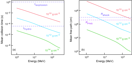
Figure 1: (a) Mean neutrino collision times $\tilde{\kappa}^{-1}$ for three mass densities (solid curves) corresponding to supernova models given in Table 1. Dashed horizontal lines indicate the characteristic explosion time $\tau_{\rm explosion}$ and hydrodynamical timescale $\tau_{\rm hydro}$ for a typical core-collapse supernova simulation. (b) Neutrino mean free path for three mass densities (solid curves). Dashed horizontal lines indicate a characteristic shock radius $R_{\rm shock}$ and radius of the protoneutron star $R_{\rm PNS}$ in a typical core-collapse supernova simulation.

For comparison, we display also a characteristic supernova explosion time and a characteristic hydrodynamical timescale in Fig. 1(a). For the highest density case of $10^{14}\mbox{\,g\,cm}^{3}$ in Fig. 1(a), we see that the mean collision time is $\sim 10^{-5}$ seconds for the lowest energies and $\sim 10^{-9}$ seconds for the highest energy. Figure 1(a) indicates that a standard explicit integration is impractical for this problem. The maximum stable explicit timestep will be governed by the fastest timescale for the neutrino interactions, which is about $10^{-9}$ seconds for the $10^{14}\mbox{\,g\,cm}^{3}$ case, but the timescale of the explosion is $\sim 1$ second. Thus a traditional explicit integration method such as the forward Euler algorithm would require billions of timesteps to integrate over the complete explosion because of the stability constraint, whereas a typical implicit calculation may require only of order hundreds of integration steps for this case, because the implicit timestep typically is limited by accuracy but not by stability.

Table 1: Conditions from supernova models Liebendorfer et al. (2004)

Model	Density $({\rm g\,cm}^{-3})$	$kT$ (MeV)	$Y_{\rm e}$
I	$1.0\times 10^{14}$	20.54	0.25
II	$1.0\times 10^{12}$	7.71	0.12
III	$1.0\times 10^{10}$	3.14	0.26

VI Neutrino Transport Regimes

Figure 1(b) shows the neutrino mean free path as a function of their energy for the models in Table 1. As expected intuitively based on the characteristic scaling of neutrino cross sections with energy and density, collisions are more common (the mean free path is shorter) at higher densities and higher energies. Estimates of the size of the protoneutron star and the supernova shock radius calculated by Bruenn (2016) are also displayed, which shows that neutrinos are trapped at the higher densities and are able to escape the protoneutron star and the shock radius for low-energy neutrinos at low densities. Thus the models that we shall calculate span the range of neutrino transport behavior from diffusion to transitional to free-streaming under core-collapse supernova conditions.

VII Explicit Algebraic Methods

Now let’s consider numerical solutions of the model from the preceding sections. We have applied to our neutrino models an adaptation of the three distinct modified explicit methods that were developed and used to solve astrophysical thermonuclear networks in Refs.  Guidry (2012); Guidry et al. (2013a); Guidry and Harris (2013); Guidry et al. (2013b); Guidry (2016); Brock et al. (2015); Haidar et al. (2016):

1. the explicit asymptotic approximation (Asy) Guidry (2012); Guidry et al. (2013a),

2. quasi-steady-state approximation (QSS) Guidry (2012); Guidry and Harris (2013), and

3. partial equilibrium approximation (PE) Guidry (2012); Guidry and Harris (2013),

where the partial equilibrium method will be used in conjunction with either the asymptotic method (Asy+PE approximation) or the quasi-steady-state method (QSS+PE approximation). In general these methods use algebraic constraints to remove the three distinct sources of stiffness appearing in generic kinetic equations that were documented in Ref. Guidry (2012), thus stabilizing the integration for (much) larger timesteps than would be possible for traditional explicit methods. For these methods applied to the neutrino transport problem our results indicate that algebraically stabilized explicit methods can take timesteps comparable to those for implicit methods, but can compute each timestep more efficiently because no matrix inversions are required. Thus, these methods hold considerable promise for faster and more efficient solution of neutrino transport equations in astrophysical explosions and mergers than are now possible. This paper introduces our neutrino evolution formalism and reports on results for the explicit asymptotic approximation, with our results with this formalism using the QSS, Asy+PE, and QSS+PE approximations to be reported separately.

VII.1 The Explicit Asymptotic Approximation

The explicit asymptotic approximation (Asy) is described in depth for thermonuclear networks in Refs. Guidry (2012); Guidry et al. (2013a). Since a thermonuclear network and the neutrino evolution network being considered here are of similar form, much of the formalism developed in Ref. Guidry et al. (2013a) applies here also with appropriate modification, and we shall highlight only the equations specific to the present neutrino formalism. Let’s solve Eq. (16) for the number density in bin $i$,

$$\mathscr{N}_{i}=\frac{1}{\tilde{\kappa}_{i}}\left(\eta_{i}-\frac{d\mathscr{N}_{i}}{dt}\right),$$ (21)

and consider the asymptotic limit $d\mathscr{N}_{i}/dt\rightarrow 0$ corresponding to $\eta_{i}\approx\tilde{\kappa}_{i}\mathscr{N}_{i}$. Using a finite-difference approximation for the derivative at a particular iteration gives

$$\frac{d\mathscr{N}_{i}^{n}}{dt}=\frac{\mathscr{N}_{i}^{n+1}-\mathscr{N}_{i}^{n}}{\Delta t}-\frac{\Delta t}{2}\frac{d^{2}\mathscr{N}^{n}_{i}}{dt^{2}}+\ldots,$$ (22)

where $\Delta t$ is the timestep and dots represent higher-order terms. This permits an approximate expression for the number density $\mathscr{N}_{i}^{n+1}$ at the $n+1$ step to be constructed from quantities known at step $n$,

$$\mathscr{N}_{i}^{n+1} =\frac{1}{\tilde{\kappa}_{i}}\left(\eta_{i}-\frac{d\mathscr{N}_{i}^{n}}{dt}\right)$$

$$=\frac{\eta_{i}}{\tilde{\kappa}_{i}}-\frac{1}{\tilde{\kappa}_{i}}\frac{d\mathscr{N}_{i}^{n}}{dt}$$

$$=\frac{\eta_{i}}{\tilde{\kappa}_{i}}-\frac{1}{\tilde{\kappa}_{i}}\left(\frac{\mathscr{N}_{i}^{n+1}-\mathscr{N}_{i}^{n}}{\Delta t}\right),$$

where only the first term in the expansion on the right side of Eq. (22) has been retained in the last step. This may be solved for $\mathscr{N}_{i}^{n+1}$ to give

$$\mathscr{N}_{i}^{n+1} =\frac{\mathscr{N}_{i}^{n}+\Delta t\eta_{i}}{1+\tilde{\kappa}_{i}\Delta t}$$

$$=\mathscr{N}_{i}^{n}+\frac{\Delta t}{1+\tilde{\kappa}_{i}\Delta t}(\eta_{i}-\tilde{\kappa}_{i}\mathscr{N}_{i}^{n})$$

$$=\mathscr{N}_{i}^{n}+\frac{\Delta tC_{i}^{n}}{1+\tilde{\kappa}_{i}\Delta t},$$ (23)

where Eq. (16) was used in the last step. This is an explicit method because $\mathscr{N}_{i}^{n+1}$ can be computed directly from quantities already known at step $n$, so no iterations with implied matrix inversions are required in the solution. It could also be viewed as a hybrid implicit–explicit or semi-implicit method because it is derived from Eq. (22), which has both $\mathscr{N}_{i}^{n+1}$ and $\mathscr{N}_{i}^{n}$ on the right hand side of the equation. In Laiu et al. (2021), Eq. (23) was used to solve Eq. (16) implicitly with fixed-point iteration, and can therefore be viewed as a single Picard step. However we choose to refer to this solution as an algebraically stabilized explicit method. We note that if $\mathscr{N}_{i}^{n}\in[0,1]$ then $\eta_{i}/\tilde{\kappa}_{i}\in[0,1]$. Then is is easy to show that $\mathscr{N}_{i}^{n+1}\in[0,1]$ for any $\Delta t$, which implies unconditional stability.

VII.2 The Explicit Forward Euler Algorithm

The simplest explicit method is the forward Euler algorithm, which when applied to Eq. (16) takes the form

$$\mathscr{N}_{i}^{n+1}=\mathscr{N}_{i}^{n}+\Delta tC_{i}^{n},\qquad C_{i}^{n}\equiv d\mathscr{N}_{i}^{n}/dt=\eta_{i}-\tilde{\kappa}_{i}\mathscr{N}_{i}^{n}.$$ (24)

Generally the explicit forward Euler method will be stable for timesteps less than a critical timestep $\tau_{\rm c}$ that is proportional to the inverse of the fastest rate in the system, $\tau_{\rm c}=2/\max(\tilde{\kappa}_{i})$, while the validity of the asymptotic approximation increases for timesteps larger than $\tau_{\rm c}$. Thus, we adopt a criterion that if the desired timestep in the numerical integration is less than $\tau_{\rm c}$ the forward Euler method of Eq. (24) is used, since it will be stable, but if the desired timestep is greater than or equal to $\tau_{\rm c}$ the explicit asymptotic approximation of Eq. (23) is used instead, since the forward Euler method would be unstable for $\Delta t\geq\tau_{\rm c}$.

VII.3 Conservation of Particle Number

Physically, it is desirable that our methods conserve particle number to machine precision. We investigate this by first considering particle number conservation for the forward Euler method, for which the total particle number $N(t)$ at time $t$ is given by

$$N(t)=\int_{\mathbb{R}^{+}}\mathscr{N}(\epsilon,t)dV_{\epsilon}\approx\sum_{i=1}^{N_{b}}\mathscr{N}_{i}(t)\Delta V_{i}^{\epsilon}.$$ (25)

Multiplying both sides of Eq. (24) by $\Delta V_{i}^{\epsilon}$ and summing over all $i$ gives

$$N^{n+1}=N^{n}+\Delta t\sum_{i=1}^{N_{b}}C_{i}^{n}\Delta V_{i}^{\epsilon}.$$ (26)

The second term in this expression vanishes because

$$\sum_{i=1}^{N_{b}}C_{i}^{n}\Delta V_{i}^{\epsilon} =\sum_{i=1}^{N_{b}}\sum_{k=1}^{N_{b}}\big{[}(1-\mathscr{N}_{i}){\mathscr{R}^{\rm in}_{ik}}\mathscr{N}_{k}$$

$$\qquad\qquad-(1-\mathscr{N}_{k}){\mathscr{R}^{\rm out}_{ik}}\mathscr{N}_{i}\big{]}\Delta V_{i}^{\epsilon}\Delta V_{k}^{\epsilon}$$ (27)

$$=\sum_{i=1}^{N_{b}}\sum_{k=1}^{N_{b}}({\mathscr{R}^{\rm in}_{ik}}-{\mathscr{R}^{\rm out}_{ki}})(1-\mathscr{N}_{i})\mathscr{N}_{k}\Delta V_{i}^{\epsilon}\Delta V_{k}^{\epsilon}=0,$$

which results from expanding summations, gathering like terms $(1-\mathscr{N}_{i})\mathscr{N}_{k}$, and noting from Eq. (6) that ${\mathscr{R}^{\rm in}_{ik}}={\mathscr{R}^{\rm out}_{ki}}$, where

$$\mathscr{R}^{\rm in/out}_{ik}\equiv{\mathscr{R}^{\rm in/out}}(\epsilon_{i},\epsilon_{k}).$$

Thus $N^{n+1}=N^{n}$ and the forward Euler algorithm conserves particle number at each timestep.

Now apply the same analysis to the explicit asymptotic approximation. The analog of Eq. (26) is

$$N^{n+1}=N^{n}+\Delta t\sum_{i=1}^{N_{b}}\frac{C_{i}^{n}}{1+\tilde{\kappa}_{i}\Delta t}\Delta V_{i}^{\epsilon},$$ (28)

and the denominator may be expanded as

$$\frac{1}{1+\tilde{\kappa}_{i}\Delta t}=\sum_{m=0}^{\infty}(-1)^{m}(\tilde{\kappa}_{i}\Delta t)^{m},$$ (29)

to obtain

$$N^{n+1} =N^{n}+\Delta t\sum_{i=1}^{N_{b}}\sum_{m=0}^{\infty}C_{i}^{n}\Delta V_{i}^{\epsilon}(-1)^{m}(\tilde{\kappa}_{i}\Delta t)^{m}$$

$$=N^{n}+\Delta t\sum_{i=1}^{N_{b}}C_{i}^{n}\Delta V_{i}^{\epsilon}$$

$$\quad+\sum_{i=1}^{N_{b}}\sum_{m=1}^{\infty}C_{i}^{n}\Delta V_{i}^{\epsilon}(-1)^{m}(\tilde{\kappa}_{i})^{m}(\Delta t)^{m+1}.$$ (30)

When $\tilde{\kappa}_{i}\Delta t<1$, this agrees with Eq. (26) up to $\mathscr{O}(\Delta t^{2})$ since the second term will vanish due to the symmetry of the kernels, as demonstrated in Eq. (27). The problem is the third term of Eq. (30): the approximation is expected to be valid for $\tilde{\kappa}_{i}\Delta t\gg 1$, so the expansion doesn’t converge and the explicit asymptotic approximation does not guarantee conservation of particle number. However, as the population density approaches equilibrium, $C_{i}^{n}\to 0$ and the third term can be small even when $\tilde{\kappa}_{i}\Delta t\gg 1$. As for the thermonuclear networks investigated in Refs. Guidry (2012); Guidry et al. (2013a); Guidry and Harris (2013); Guidry et al. (2013b), we may deal with this by regulating the timestep such that the integration yields conservation of particle number at an acceptable level for a given problem, when employing the explicit asymptotic approximation.

VII.4 Integration Timestep Control

As we have shown above, our explicit algebraic algorithms have the disadvantage that they are not all guaranteed to conserve particle number, but the error in particle number is controlled by the integration timestep size. Thus in the FENN algorithms for neutrino population evolution (and in the FERN algorithms for thermonuclear networks) timesteps are chosen such that at each point in the calculation the particle number is conserved locally within a tolerance specified by user-defined parameters, with those parameters chosen such that integrated global error in particle number is conserved to acceptable tolerance for the entire calculation (with acceptable error tolerance dictated by the nature of the problem being integrated).

For the first integration timestep $\Delta t_{0}$ a suitable guess is used (for example $\Delta t_{0}=0.01t_{0}$, where $t_{0}$ is the initial time) for a trial timestep, and at each timestep after the first we choose a trial timestep predicted by the previous timestep (as described below). For each integration timestep two calculations are performed, one for the full trial timestep and one for two successive timesteps, each equal to half the trial timestep. We then accept provisionally the results of the two half timesteps and test for particle number conservation. If the local tolerance conditions are satisfied, the timestep is accepted. If the error is too large an iteration on the preceding algorithm is performed for successively smaller timesteps until the tolerance condition is satisfied and that timestep is accepted. Conversely, if the error is judged too small for maximum efficiency with acceptable error in the initial comparison, the iteration increases the timestep accordingly. The code has the capability to recalculate reaction rates at each step of this iteration, but in the present calculations we recalculate fluxes for each iteration but use the same reaction rates for all calculations within the timestep. We then use comparison of errors for the two half timestep and full timestep approximations of the accepted solution to estimate a local derivative of error with respect to timestep size, and use that to project a trial timestep for the next integration step that is expected to have acceptable error. This procedure is repeated at each integration timestep of the calculation.

VIII Calculations and Comparisons

We shall now present comparisons of numerical solutions using the explicit asymptotic method and those from several standard numerical methods appropriate for stiff systems. The models given in Table 1 correspond to representative conditions in various zones of a core-collapse supernova simulation. The standard test problem will assume the neutrino particle densities to be distributed over 40 energy bins, and for each case we integrate the relaxation of an initial strongly peaked gaussian distribution to the equilibrium Fermi–Dirac distribution, as illustrated schematically in Fig.  2.

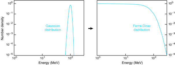
Figure 2: Test problem examined in this paper: relaxation of an initial gaussian neutrino energy distribution to a Fermi–Dirac distribution through neutrino–electron scattering. Calculations were performed for the three temperature–density environments listed in Table 1.

As representative examples, timestepping and error plots (violation of particle-number conservation) for the high-density Model I and low-density Model III from Table 1 are displayed in Figs. 3 and 4.

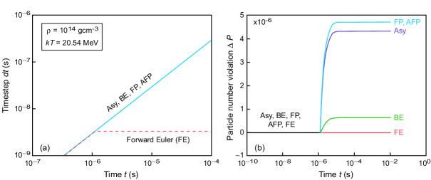
Figure 3: (a) Integration timestep versus time for the high-density ($\rho=1\times 10^{14}{\rm\ g\,cm}^{-3},\ kT=20.54{\rm\ MeV}$) Model I of Table 1 using explicit asymptotic (Asy), backward Euler (BE), fixed point (FP), accelerated fixed point (AFP), and forward Euler (FE) methods Laiu et al. (2021). Parameters were chosen so that each of these methods (except for forward Euler) follows essentially the same timestepping curve $dt$ versus $t$. Details concerning the backward Euler, fixed point, and accelerated fixed point calculations may be found in Ref. Lackey-Stewart (2020). (b) Violation of particle number conservation $\Delta P$ versus time for the cases in (a) in units of $10^{-6}$. The timestepping curves in (a) for all methods except forward Euler are virtually identical, and the final violation of particle number conservation in (b) ranges over negligible for forward Euler, $\sim 1\times 10^{-6}$ for backward Euler, and $\sim 4.5\times 10^{-6}$ for the asymptotic, fixed point, and accelerated fixed point methods.

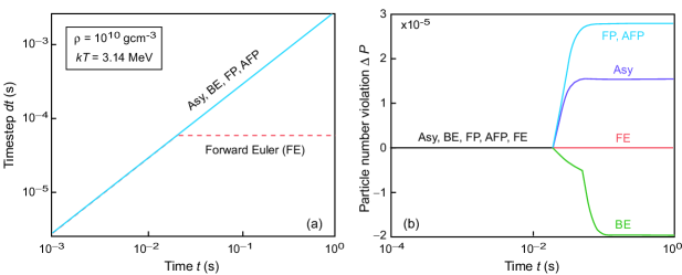
Figure 4: (a) Integration timestep versus time for the low-density ($\rho=1\times 10^{10}{\rm\ g\,cm}^{-3},\ kT=3.14{\rm\ MeV}$) Model III of Table 1 using explicit asymptotic (Asy), backward Euler (BE), fixed point (FP), accelerated fixed point (AFP), and forward Euler (FE) methods. Parameters were chosen so that each of these methods (except for forward Euler) follows essentially the same timestepping curve $dt$ versus $t$. Details concerning the backward Euler, fixed point, and accelerated fixed point calculations may be found in Ref. Lackey-Stewart (2020). (b) Violation of particle number conservation $\Delta P$ versus time for the cases in (a) in units of $10^{-5}$. The timestepping curves in (a) for all methods except forward Euler are virtually identical, and the final violation of particle number conservation in (b) ranges over negligible for forward Euler to approximately $-2\times 10^{-5}$ for backward Euler, $1.5\times 10^{-5}$ for asymptotic, and $3\times 10^{-5}$ for both fixed point and accelerated fixed point methods.

Our results show in general that for evolution of neutrino energy distributions the explicit asymptotic method is capable of stable integration timesteps comparable in size to those of standard implicit methods, because the algebraic constraints remove substantial stiffness from the system of equations. In particular, we find that

1. The algebraically stabilized explicit approach overcomes the disastrous stability restriction that prevents increasing the timestep beyond a certain time in the integration imposed generically by the stability constraint of standard explicit methods; compare the forward Euler and explicit asymptotic timestepping curves in Figs. 3(a) and 4(a).

2. When parameter choices yield similar timestepping for explicit asymptotic and standard implicit methods, the errors in the calculated neutrino densities for the asymptotic method are the same order of magnitude as the errors for standard implicit methods; see the particle-number conservation error curves shown in Figs. 3(b) and 4(b).

Explicit methods can compute each timestep more efficiently than implicit methods since no matrix inversions are required. This, coupled with the comparable timestepping demonstrated in Figs. 3(a) and 4(a), indicates that the explicit asymptotic method for neutrino transport has the capability to out-perform standard implicit methods, particularly for larger networks since the cost of matrix inversion increases rapidly with size of the matrices. This result is consistent with those found previously for thermonuclear networks of similar structure as the present neutrino transport network Guidry (2012); Guidry et al. (2013a); Guidry and Harris (2013); Guidry et al. (2013b); Feger (2011); Chupryna (2008); Brey (2022); Brock et al. (2015); Haidar et al. (2016); Guidry et al. (2023); Brey et al. (2023), but that were often larger and of even greater stiffness.

IX Speed versus Accuracy for Explicit Algebraic Methods

Having established in some simple examples that the explicit asymptotic method shows promise for describing the evolution of neutrino populations, let us turn to a more detailed and quantitative comparison of explicit asymptotic simulations with traditional ones. In Fig. 5

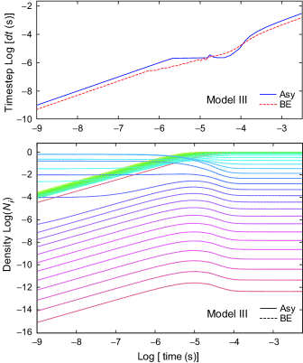
Figure 5: Neutrino number densities $\mathscr{N}_{i}$ for 40 energy bins as a function of time $t$ given in seconds, calculated for the evolution of an initial gaussian distribution to a final Fermi–Dirac distribution at equilibrium as in Fig. 2, for Model I in Table 1. (Lower Panel) Number density $\mathscr{N}_{i}$ versus time $t$ in seconds. Solid curves represent explicit asymptotic (Asy) results and dashed curves correspond to reference backward Euler (BE) implicit calculations. (Upper Panel) Timestepping for the calculation displayed in lower panel for the asymptotic approximation (Asy) and for the reference backward Euler calculation (BE). Calculations were performed with the FENN C++ codebase, except that reference backward Euler results were calculated using a standard integration routine in MatLab.

we illustrate the evolution of an initial gaussian energy distribution to a final Fermi–Dirac distribution (see Fig. 2) for the temperature and density environment of Model I in Table 1. We see that the explicit asymptotic calculation maintains competitive timestepping relative to a standard implicit backward Euler calculation across the entire calculation, while exhibiting rather good agreement with benchmark implicit calculations for the evolution of the neutrino densities. Since explicit methods can compute each timestep faster than implicit methods, this suggests that these new explicit methods could be faster than standard implicit ones for computing the evolution of neutrino energy distributions in events such as core collapse supernova explosions and neutron star mergers.

However, we have noted above that the explicit asymptotic method is an approximation for which the amount of error introduced by the approximation can be controlled by placing restrictions on the timestepping. Thus we must address systematically whether the accuracy with competitive timestepping for explicit algebraic methods illustrated in Figs. $\ref{fig:compareHighDens}-\ref{fig:timestepAndEnergyBins}$ is sustainable over a range of realistic scenarios. With that in mind, let us turn to a systematic analysis of error versus speed in explicit asymptotic evolution of neutrino populations.

IX.1 Controlled and Poorly Controlled Approximations

As elaborated in Refs.  Guidry (2012); Guidry et al. (2013a); Guidry and Harris (2013); Guidry et al. (2013b); Guidry (2016); Brock et al. (2015); Haidar et al. (2016) and the present paper, explicit algebraic methods are designed for use in large-scale astrophysical simulations where typically a multi-dimensional radiation hydrodynamics code is coupled in real time to neutrino transport and/or thermonuclear burning kinetic networks. Often in such calculations evolving a realistic neutrino or thermonuclear network can dominate the computing budget, necessitating approximations. In such an environment we desire that approximations in the kinetic networks entail uncertainties smaller than the total errors and uncertainties from all other sources in the calculation. A reasonable criterion with present technology is that errors of a few percent or less are acceptable for approximate kinetic networks coupled to fluid dynamics. Here we have given examples that explicit asymptotic methods can give errors less than this threshold while exhibiting timestepping comparable to that for standard implicit methods. For example, in Figs. 3 and 4 the explicit asymptotic error in number-density conservation (a measure of average error in individual neutrino densities) is of order $10^{-5}$ to $10^{-6}$ for timestepping equivalent to that of implicit methods, and Fig. 5 will exhibit good agreement of explicit asymptotic and implicit methods with comparable timestepping. This suggests that integration of neutrino kinetic equations can be made more efficient by trading

• a poorly controlled approximation, common in current large-scale simulations (sufficient truncation and approximation of realistic networks to allow them to be integrated quickly enough with standard methods),

• for a controlled approximation (algebraically stabilized explicit algorithms applied to networks of realistic size and complexity, with a quantitative error constraint dictated by the physics of the problem).

By such means, it should be possible to integrate many physically realistic problems that are presently intractable using standard algorithms on existing machines. This method of trading speed against accuracy for explicit algebraic approximations is documented in Ref. Guidry et al. (2023) for thermonuclear networks. We now investigate the tradeoff of speed for accuracy in explicit asymptotic neutrino simulations. Let’s begin by defining quantitative measures of speed and accuracy.

IX.2 A Quantitative Measure of Accuracy

Explicit algebraic methods employ approximations of the realistic problem, so the algorithm itself introduces some level of error. For example, we showed in Section VII.3 that the asymptotic approximation does not conserve particle number exactly. To examine the implications of employing an approximate solution one needs a systematic measure of the error associated with the approximation. We may characterize the accuracy of an explicit algebraic evaluation of the neutrino evolution by integrating deviation of the neutrino number densities $\mathscr{N}_{i}$ from benchmark results (which are taken to be exact), and computing the root mean square deviation in number densities summed over all species (energy bins) at that time. This difference results in residuals $R_{i}(t)$ for each species $i$ in the network at every time $t$,

$$R_{i}(t)\equiv|\mathscr{N}_{i}(t)-\mathscr{N}_{i}^{0}(t)|,$$ (31)

where $\mathscr{N}_{i}(t)$ is the explicit asymptotic approximation for the number density in bin $i$ at time $t$ and $\mathscr{N}_{i}^{0}(t)$ is the corresponding exact result. The root mean square (RMS) error $R(t)$ summed over all bins at time $t$ is then defined by

$$R(t)\equiv\sqrt{\sum_{i}R_{i}(t)}=\sqrt{\sum_{i}|\mathscr{N}_{i}(t)-\mathscr{N}_{i}^{0}(t)|^{2}},$$ (32)

where the sum is over all energy bins and $\sum_{i}\mathscr{N}_{i}^{0}=1$. It will be shown later that the error $R(t)$ is typically finite only over a limited range of integrations times. The total error per unit time $\mathscr{E}$ for integrating the network to equilibrium is then approximated as

$$\mathscr{E}=\frac{1}{\delta t}\sum_{j=j_{0}}^{j(t_{\rm eq})}R(t_{j})\,\delta t_{j},$$ (33)

where $t_{j}$ is the time at the $j$th plot output step, $R(t_{j})$ is given by Eq. (32), $j_{0}$ is the first plot output step with finite $R(t)$, $j(t_{\rm eq})$ is the plot output step corresponding to the equilibration time, $\delta t_{j}=t_{j}-t_{j-1}$ is the time difference between the $j$th and $(j-1)$th plot output steps, and $\delta t\equiv t_{\rm eq}-t(j_{0})$ is the total time between onset of finite $R(t)$ and equilibration at $t_{\rm eq}$. The error $\mathscr{E}$ computed from Eq. (33) may be taken as a single number characterizing the global accuracy of a given calculation.

IX.3 A Quantitative Measure of Speed

To evaluate the utility of explicit algebraic methods one needs a systematic measure of how long a calculation requires, relative to standard methods. The speed of a calculation can be parameterized conveniently in terms of the total number of integration steps required to complete a given simulation. This is an “intrinsic” measure, since it should be largely independent of computing platform. The total integration time is then a function of the number of steps and the time required for each step. Because standard implicit methods such as backward Euler typically take longer than an explicit method to compute each step,

1. if the algebraically stabilized explicit method requires a similar number or fewer integration steps than an implicit method, it will likely be faster, but

2. if it takes more integration steps than the implicit method, whether the implicit or algebraic explicit method is faster will depend on the time to compute each timestep, which is platform dependent.

The time to compute an explicit timestep relative to that for an implicit timestep on the same platform depends primarily on the additional linear algebra overhead incurred by the implicit method because of the required matrix inversions, which increases with network size. If the difference between explicit and implicit methods is approximated as being due entirely to the additional linear algebra overhead of the implicit method, then a speedup factor may be defined as $F\equiv 1/(1-f)$, where $f$ is the fraction of overall computing time spent by the implicit code in its linear algebra solver during a timestep. Then we may expect that the explicit algebraic code can compute a single timestep approximately $F$ times faster than an implicit code in a given computational environment.

The factor $F$ has been computed as a function of network size for thermonuclear networks in Ref. Guidry et al. (2013a), using the implicit backward Euler code Xnet Hix and Thielemann (1999) with a variety of linear solvers. The present neutrino network is similar in structure to a thermonuclear network, except that the neutrino network reaction matrix is dense but larger thermonuclear networks have quite sparse reaction matrices. However, the results for $F$ tabulated in Ref. Guidry et al. (2013a) in networks as small as 40 isotopes were determined using a dense-matrix solver in Xnet. Thus we may expect that for the present 40-species neutrino network the value $F\sim 4$ inferred in thermonuclear networks is approximately valid and we shall assume in this discussion that the explicit asymptotic method can compute each timestep $\sim 4$ times faster than a corresponding implicit method on the same machine. Then the ratio of times required for integration of a given problem with explicit asymptotic and implicit backward Euler methods may be estimated as

$$\frac{\Delta t_{\rm EA}}{\Delta t_{\rm BE}}\simeq\frac{S_{\rm EA}}{F\cdot S_{\rm BE}}\simeq 0.25\,\left(\frac{S_{\rm EA}}{S_{\rm BE}}\right),$$ (34)

where $\Delta t$ denotes elapsed wallclock time for the complete integration, $S$ is the number of integration steps, “EA” labels quantities from the explicit asymptotic calculation, “BE” labels quantities from the backward Euler calculation, and we have assumed a speedup factor $F\sim 4$ for the 40-species neutrino network employed in this work.

X Trading Speed for Accuracy in Realistic Simulations

Let us now use the tools developed in Section IX to evaluate speed versus accuracy for some explicit asymptotic (Asy) simulations of neutrino population evolution, using the simplified model described above that limits interactions to neutrino–electron scattering. The benchmark that we shall employ for comparison is an integration of the 40-species neutrino network using a standard implicit backward Euler algorithm, under the same conditions as for the Asy calculation. Figure 6

Figure 6: Speed versus accuracy using explicit algebraic methods for evolution of neutrino energy distributions. In each plot 40 discrete energy bins for the neutrinos are tracked in time, assuming the only interaction to be neutrino–electron scattering. Models I, II, and III are defined in Table 1. Solid curves are explicit asymptotic (Asy) calculations with timestepping parameters adjusted to emphasize speed (lower panels) versus accuracy (upper panels). This tradeoff can be adjusted continuously but for display purposes we have chosen three discrete parameter sets for each model, labeled “Accurate”, “Intermediate”, and “Fast”, with Accurate being slower but more accurate, Fast being faster but less accurate, and Intermediate being intermediate in speed and accuracy. Specifically, all parameters controlling the timestepper described in Section VII.4 were fixed for a given model, except that we varied the single parameter specifying the allowed deviation from particle number conservation in one timestep for the asymptotic approximation to dial the “Accurate”, “Intermediate”, and “Fast” cases. Dashed curves are reference calculations using an implicit backward Euler algorithm (labeled “ BE”). In most cases the solid and dashed curves are indistinguishable visually plotted at this scale, with the exception of the Model III Fast Case, where small differences can be seen. The number of explicit asymptotic integration steps required is given as an integer at the bottom of each plot and that is followed in parentheses by the error calculated from Eq. (33), given as a percentage. The number of integration steps required for the backward Euler (BE) reference integration was 54 steps for Model I, 64 steps for Model II, and 88 steps for Model III. All explicit Asymptotic calculations were performed with the FENN C++ codebase. Backward Euler reference curves were calculated with a standard integration package in MatLab.

illustrates the tradeoff of speed versus accuracy for some explicit algebraic calculations. In this figure the three columns of plots correspond to conditions associated with Models I, II, and III, respectively, in Table 1, while the three successive rows of plots illustrate different choices of control parameters in the explicit asymptotic calculation that lead to decreasing speed but higher accuracy for vertically successive plots.

Each plot is labeled near the bottom by the number of explicit asymptotic integration steps required, followed in parentheses by the RMS error per unit time $\mathscr{E}$ (expressed as a percentage) calculated from Eq. (33) for the explicit algebraic calculation relative to the reference benchmark. For example, in the third column of plots in Fig. 6 (corresponding to Model III from Table 1), for successive plots from the top the number of explicit algebraic integration steps required decreases from 236 to 116 to 71, while the error increases from 0.093% to 0.103% to 0.213%. Thus in this simple example we have gained a factor of more than three in speed at the expense of increasing the error by a little over a factor of two in dialing the integration parameters between “Accurate” and “Fast” sets, with the error in the “Fast” calculation still quite acceptable for coupling to a hydrodynamical simulation by our earlier arguments.

The number of explicit asymptotic timesteps and the errors for all cases in Fig. 6 are summarized in Table 2. From Fig. 6 and Table 2, the bottom row of plots in Fig. 6 may be characterized as faster but less accurate, the top row as slower but more accurate, and the middle row as intermediate in both speed and accuracy. We have exhibited the tradeoff of speed versus accuracy with three discrete examples in the rows of Fig. 6, but a continuum of possible parameter choices could be used to dial this tradeoff, as suggested by the double vertical arrow on the right side of Fig. 6. Let us now discuss in more depth the tradeoff of speed versus accuracy illustrated in Fig. 6.

X.1 Accuracy of the Explicit Algebraic Approximation

The primary contribution to error in Eq. (33) tends to occur in restricted ranges of integration time, with the error being negligible over much of the rest of the calculation. For example, in Fig. 7

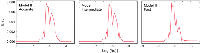
Figure 7: Root mean square error $R(t)$ from Eq. (32) plotted versus time for the three Model II cases shown in Fig. 6. For these examples almost all of the error accumulates between $\log t=-6$ and $\log t=-4$.

we display the RMS error $R(t)$ from Eq. (32) as a function of time for the Accurate, Intermediate, and Fast calculations of Model I that are displayed in Fig. 6. In these examples we see that almost all of the error accumulates between $t\sim 10^{-6}$ and $t\sim 10^{-4}$ seconds. In an operator-split coupling to hydrodynamics the continuous integration ranges used as illustration in Fig. 6 would be broken up into a series of sequential piecewise integrations for a given fluid zone, with each piece representing integration of the network over one hydro timestep in the zone. Thus, significant error from the neutrino network for that zone will occur for only a restricted range of hydrodynamical integration steps (those lying roughly between $10^{-6}$ and $10^{-4}$ seconds of elapsed fluid integration time in the preceding example). We note that this could be used to optimize the tradeoff of speed versus accuracy even further on a zone by zone basis in the coupled hydro–kinetic system. We leave such optimizations for future applications of the basic ideas presented here to specific problems.

Of fundamental interest is a translation of neutrino network errors $\mathscr{E}$ defined in Eq. (33) and displayed in Fig. 6 and Table 2 into an overall error introduced into the coupled kinetic–hydrodynamical system by the explicit algebraic approximations. The error computed from Eq. (33) may be interpreted as the RMS error per unit time, over the range of times for which $R(t)$ is finite. Therefore, no error is introduced for those hydro integration steps that do not overlap the regions of significant $R(t)$ in Fig. 7. For those hydro timesteps that do overlap regions of significant $R(t)$, the error introduced by network approximations for a hydro timestep $\Delta t_{\rm hydro}$ will depend on the integrated value of $R(t)$ over the hydro timestep, with the hydro timestep depending on factors such as the method of hydro integration, zone sizes, and fluid characteristics at that time. Thus it is case specific. Nevertheless the relatively small values of $\mathscr{E}$ that can be chosen in Fig. 6 suggest that the maximum overall error can be controlled to a few percent or less while maintaining adequate speed, when this formalism is applied to specific problems.

X.2 Speed of the Explicit Algebraic Approximation

The total time to integrate a problem is a function of the number of timesteps required and the time required to compute each timestep, with explicit methods generally computing a timestep faster than a corresponding implicit method. For each of the cases in Fig. 6, we may use the number of integration steps required for the explicit asymptotic calculation and for a corresponding implicit backward Euler calculation in conjunction with Eq. (34) to make a rough estimate of the overall relative speed of the explicit asymptotic and implicit calculations. Implicit backward Euler calculations required 54, 64, and 88 steps for integrating Models I, II, and III, respectively, over the time ranges in Fig. 6, and the required asymptotic integration steps are given for each model and case in Fig. 6 and Table 2.

Table 2: Timesteps and errors $\mathscr{E}$ from Eq. (33) for Fig. 6

	MODEL I	MODEL II	MODEL III
Case	Steps   Error	Steps   Error	Steps   Error
Accurate	278      0.080%	160    0.044%	236    0.093%
Intermediate	186      0.138%	114    0.045%	116    0.103%
Fast	123      0.191%	71      0.047%	71      0.213%

As an example, consider the rightmost column of plots in Fig. 6 corresponding to Model III, for which the backward Euler implicit calculation required 88 integration steps. Then from Eq. (34), for the Accurate calculation (top row) the number of Asy integration steps required is 236 and the ratio of wallclock times for asymptotic integration relative to implicit integration on equivalent machines may be estimated as

$$\frac{\Delta t_{\rm EA}}{\Delta t_{\rm BE}}\simeq 0.25\times\frac{236}{88}\simeq 0.67.$$

Thus, for the Accurate calculation of Model III the explicit asymptotic integration is expected to be approximately $(0.67)^{-1}\simeq 1.5$ times as fast as the backward Euler calculation run on the same hardware. (The explicit method requires $\sim 2.7$ times as many integration steps, but computes each step $\sim 4$ times faster than the implicit method.) For the Intermediate Model III example a similar calculation gives

$$\frac{\Delta t_{\rm EA}}{\Delta t_{\rm BE}}\simeq 0.25\times\frac{116}{88}\simeq 0.33,$$

so the Intermediate calculation is estimated to be about $(0.33)^{-1}\simeq 3$ times faster than the implicit BE calculation, while for the Fast Model III example

$$\frac{\Delta t_{\rm EA}}{\Delta t_{\rm BE}}\simeq 0.25\times\frac{71}{88}\simeq 0.20,$$

and the Fast asymptotic calculation is estimated to be about $(0.20)^{-1}\simeq 5$ times faster than the implicit BE calculation.

Table 3

Table 3: Ratio of Asy to BE speeds in Fig. 6

Case	Model I	Model II	Model III
Accurate	0.78	1.6	1.49
Intermediate	1.16	2.25	3.03
Fast	1.76	3.61	4.96

summarizes the estimated overall speed of the explicit asymptotic (Asy) integration relative to backward Euler (BE) integration calculated from Eq. (34) for all cases in Fig. 6. On a single CPU the explicit asymptotic calculation is similar in speed to the implicit calculation for the “Accurate” calculations but is estimated to be 1-3 times faster than the implicit calculations for the “Intermediate” calculations, and faster than the implicit calculation by factors of approximately $~{}2-5$ for the various “Fast” calculations in Fig. 6.

The numbers in Table 3 are estimates but these results illustrate how explicit algebraic methods can be used to trade speed against the accuracy needed for a particular application in a controlled way. If one is coupling to a hydrodynamical simulation of say a stellar explosion, then errors in the kinetic network of a few percent or less would likely be acceptable, given the errors and uncertainties associated with the whole system. Thus, Table 3 indicates that the “Intermediate” and “Fast” calculations of Fig. 6 (middle and bottom row of plots) can compute our simple neutrino network $\sim 2-5$ times faster than an implicit code (on a single CPU), with error that is likely acceptable for coupling to hydrodynamics. This advantage will grow for larger neutrino networks (more energy bins), since the Asy method requires no matrix inversions. As we shall discuss in Section XI, this advantage on a single CPU can increase dramatically if explicit algebraic approximations for kinetic networks are deployed in parallel on GPUs.

It should be noted that methods such as fixed-point or accelerated fixed-point that require no matrix inversions are faster than backward Euler methods for the problems addressed here Laiu et al. (2021), so they would likely compare more favorably than BE with our explicit algebraic calculations. However, our purpose here is not a detailed comparison of methods but rather to demonstrate that explicit algebraic methods are generally competitive with currently used algorithms for evolution of neutrino populations, and could offer significant advantages, particularly when deployed on GPUs for large networks.

XI GPU Acceleration

The present test cases for neutrino networks were implemented on single CPUs but we are porting our new explicit algebraic neutrino code to GPUs. It has been shown in prior tests with thermonuclear networks that these explicit algebraic methods are extremely amenable to GPU acceleration because of their simplicity, which implies minimal memory footprint and communication overhead. For example, we have shown using an NVIDEA K40 (Kepler) GPU that for a realistic 150-isotope thermonuclear network coupled through 1604 reactions under Type Ia supernova conditions, $\sim 600$ independent networks could be deployed in parallel and integrated on a single GPU in the same wall-clock time that a traditional implicit code could integrate one such network Guidry (2016); Brock et al. (2015); Haidar et al. (2016).

The thermonuclear networks investigated in Refs. Guidry (2012); Guidry et al. (2013a); Guidry and Harris (2013); Guidry et al. (2013b); Feger (2011); Chupryna (2008); Brey (2022); Brock et al. (2015); Haidar et al. (2016); Guidry et al. (2023); Brey et al. (2023) and the neutrino networks investigated here are structurally similar except that matrices associated with larger thermonuclear network are more sparse than those for the neutrino network. Therefore, we expect that the explicit algebraic neutrino network is also likely to realize large efficiency gains when deployed on GPUs. Since the most powerful modern supercomputers acquire the bulk of their speed from GPU accelerators, this bodes well for implementation of these new methods in future petascale and exascale applications.

XII Further Development

The results presented here have offered proof of principle with a simple model that explicit algebraic methods may provide some advantages in describing the evolution of neutrino populations in stellar explosions and mergers. As noted in the Introduction, this paper is the first step in developing and documenting the codebase FENN (Fast Explicit Neutrino Network) for neutrino transport simulations in events like core collapse supernovae and binary neutron star mergers. Several additional steps are required to convert this proof of principle into a fully usable tool.

• The neutrino couplings must be extended beyond neutrino–electron scattering to include the full complement of expected neutrino–matter interactions.

• This paper addresses only the explicit asymptotic (Asy) method of the explicit algebraic approximation. In future work we will test the quasi-steady state (QSS) and the partial equilibrium (PE) methods also for neutrino networks. Although in the examples discussed here the Asy approximation was adequate, prior experience with thermonuclear networks suggests that in more general situations the full set of Asy, QSS, and PE approximations may prove useful for the neutrino problem when the full range of neutrino–matter interactions is included.

• The examples presented here have used networks containing 40 “species” (neutrino energy bins). In future work we will investigate the scaling of execution time with number of species for the explicit algebraic neutrino network. This scaling has been established for thermonuclear networks in earlier work Guidry (2012); Guidry et al. (2013a), but not yet for neutrino networks. Because no matrix inversions are required, we may expect that the explicit algebraic methods will scale more favorably with network size than implicit methods, but we may expect some differences with the scaling found in thermonuclear networks because the matrices corresponding to large thermonuclear networks are more sparse than the matrices corresponding to the neutrino network.

• The FENN codebase will be ported to GPUs and optimized for the CPU–GPU architectures common on current petascale and exascale machines. We have laid the groundwork for that in Refs. Brock et al. (2015); Haidar et al. (2016) for explicit asymptotic thermonuclear networks using CUDA C code running on Nvidia GPUs, but that formalism must be adapted to neutrino networks and adapted to other GPUs.

• Once explicit algebraic GPU versions are in place for neutrinos, we intend to investigate the interface of FENN codes for neutrino networks (and FERN codes for thermonuclear networks Guidry (2012); Guidry et al. (2023)) with multidimensional radiation hydrodynamics codes. Many such codes are written primarily in FORTRAN (for example, Chimera Bruenn et al. (2020), FLASH Fryxell et al. (2000), GenASiS Budiardja and Cardall (2019), and thornado Pochik et al. (2021); Laiu et al. (2021)), so this work will entail meshing the primarily C++ coding of FENN for neutrino networks and FERN for thermonuclear networks with the largely FORTRAN implementation of the hydrodynamics codes.

We then anticipate that these FENN and/or FERN tools may be used to simulate events like Type Ia (thermonuclear) supernovae, core collapse supernovae, binary neutron star mergers, nova explosions, and X-ray bursts, using neutrino and/or thermodynamics kinetic networks having physically realistic size and sophistication.

XIII Summary and Conclusions

We have demonstrated for a representative neutrino transport problem that an explicit asymptotic approximation leads to controlled errors that are of acceptable size for coupling to large-scale hydrodynamics simulations, while displaying timestepping that is competitive with standard implicit methods. Since explicit methods can compute each timestep more efficiently than implicit methods because they do not require matrix inversions, the explicit asymptotic method for neutrino transport shows promise of being faster and more efficient than standard implicit methods in many large-scale simulations. Furthermore, we may expect the relative advantage of these new explicit methods to increase for larger networks because they avoid matrix inversions, and for deployment on GPUs because they entail relatively small memory and communication requirements. Thus, we propose that algebraically stabilized explicit methods may be capable of integrating many realistic neutrino (and thermonuclear) networks coupled to multidimensional hydrodynamics on existing high-performance platforms.

With the proliferation of exascale machines and the development of algebraically stabilized explicit algorithms optimized for petascale and exascale architectures, it may be expected that even more realistic simulations will become possible. To that end, we are developing two primarily C++ codebases to exploit explicit algebraic methods:

• FENN (Fast Explicit Neutrino Network) for explicit algebraic solutions of astrophysical neutrino networks, described in this paper and Ref. Lackey-Stewart (2020), and

• FERN (Fast Explicit Reaction Network) for explicit algebraic solutions of astrophysical thermonuclear networks, described in Refs. Guidry (2012); Guidry et al. (2013a); Guidry and Harris (2013); Guidry et al. (2013b, 2023).

These packages will be made available to the astrophysics community as documented open-source code for rapid solution of large kinetic networks coupled to fluid dynamics, and to the broader scientific community as an open-source template for problems in various disciplines that could profit from the scaling and efficiency gains inherent in algebraically stabilized explicit integration, particularly when they are deployed on modern GPUs.