Pseudo-Differential Sweeping Method for Ultrasound Waves with Fractional Attenuation

Abstract

We derive a pseudo-differential factorization of the wave operator with fractional attenuation. This factorization allows us to approximately solve the Helmholtz equation via a two-way (transmission and reflection) sweeping scheme tailored to high-frequency wave fields. We provide explicitly the three highest order terms of the pseudo-differential expansion to incorporate the well-known square-root first order symbol for wave propagation, the zeroth order symbol for amplitude modulation due to changes in wave speed and damping, and the next symbol to model fractional attenuation. We also propose wide-angle Padé approximations for the pseudo-differential operators corresponding to these three highest order symbols. Our analysis provides insights regarding the role played by the frequency and the Padé approximations in the estimation of error bounds. We also provide a proof-of-concept numerical implementation of the proposed method and test the error estimates numerically.

Keywords— Wave propagation, acoustics, high frequency, Helmholtz equation, pseudodifferential calculus

1 Introduction

The present study is motivated by the application of ultrasound waves to medical therapeutics and diagnosis where computational simulations are playing an increasingly important role [8, 9, 18, 59, 68, 10, 55, 41, 40]. To unleash the full potential of computer simulations of ultrasound fields, the computational method employed to run the simulations must strike the right balance between accuracy and speed. Most computational methods for ultrasound lie at one of two extremes. At one extreme, closed-form methods provide tremendous computational speed but sacrifice too much accuracy. These over-simplified methods are only valid under stringent assumptions and render a multitude of inaccuracies for realistic biological media [71, 68, 53, 30, 58, 72, 42]. At the other extreme, full-waveform simulations based on differential equations are very accurate but suffer serious scalability limitations, especially at ultrasonic MHz frequencies. In addition to short wavelengths, ultrasound waves in biological media are characterized by their fractional or power-law attenuation profiles which further complicates the validity of closed-form methods and the scalability of full-waveform simulations [51, 4, 5, 38, 20, 34, 44, 35]. This challenge (recognized by several research groups [68, 28, 39, 29, 33, 14]) exposes an unresolved need to simulate ultrasound fields efficiently enough for some clinical environments.

In most ultrasound medical applications, the transducer is designed to emit waves moving along a dominant direction of propagation. Such is the case for plane waves and beams. Some processing methods (such as ray and wavefront tracing, one-way, parabolic, paraxial, kinetic, and Eikonal models) rely on this geometry of propagation to reduce computational costs [32, 17, 16, 23, 60, 67, 22, 62, 36, 54, 11, 28]. In the present work, we pursue a similar line of work. We propose a sweeping algorithm based on a pseudo-differential factorization of the wave equation to improve the accuracy of closed-form methods while keeping the execution times much more competitive than full-waveform simulations. The pseudo-differential calculus allows us to take advantage of the geometry of acoustic energy flow, incorporate physical interactions such as transmission, reflection and attenuation while efficiently handling the highly oscillatory nature of ultrasound waves. We extend related approaches by Stolk and Op’t Root [60, 54] by considering the pseudo-differential calculus to all orders, implementing a two-way model to account for reflections, and deriving the pseudo-differential symbol for fractional attenuation. This latter feature is important for applications in biomedicine where fractional or power-law attenuation models have been shown to represent biological media accurately [66, 5, 34, 10, 20]. Our work can also be understood as an alternative to the Bremmer series which has been used for the theoretical analysis and computational treatment of multi-dimensional inverse scattering problems [57, 47].

This paper is structured as follows. In Section 2, we develop the pseudo-differential factorization of the wave equation with a fraction attenuation term, carry out the calculations for the classical decomposition of the pseudo-differential operators in inverse powers of the frequency $\omega$, and propose high order (or so-called wide-angle) Padé approximations for the pseudo-differential operators corresponding to the highest degree symbols. This development includes the well-known square-root symbol to model one-way wave propagation, the zeroth degree symbol for amplitude modulation due to changes in wave speed and damping, and the next symbol to model fractional attenuation. In Section 3, we incorporate the approximated symbols into the proposed two-way sweeping methods. Section 4 contains basic error analysis at the continuous level and provides insights concerning the role played by the frequency $\omega$ and the Padé approximations in the estimation of error bounds. In Section 5 we provide a proof-of-concept numerical implementation of the proposed method and test the error estimates numerically. Finally, in 6 we offer some concluding remarks, discuss limitations of the proposed pseudo-differential method and areas of potential improvement.

2 Pseudo-differential factorization of the wave equation

Our approach has evolved from our experience with the formulation and implementation of absorbing boundary conditions for waves [31, 3, 70, 37, 2, 69, 1, 7, 6]. The starting point is Nirenberg’s factorization theorem for hyperbolic differential operators [52, 13, 12, 2]. We consider the wave operator,

$$\mathcal{L}u =\Delta u-c^{-2}\partial_{t}^{2}u-a\partial_{t}u-a_{\alpha}\partial_{t}^{\alpha}u$$

$$=\partial_{x}^{2}u+\Delta_{\perp}u-c^{-2}\partial_{t}^{2}u-a\partial_{t}u-a_{\alpha}\partial_{t}^{\alpha}.$$ (1)

Here, $c$ is the wave speed, $a$ is the damping coefficient, $a_{\alpha}$ is the attenuation coefficient for the fractional term, and $0<\alpha<1$, is the fractional exponent of the attenuation. The Laplacian $\Delta=\partial_{x}^{2}+\Delta_{\perp}$ is decomposed to design a sweeping method that conforms to the flow of the acoustic energy imposed by ultrasound transducers along the $x$-axis. $\Delta_{\perp}$ is known as the tangential Laplacian for the hyperplane perpendicular to the $x$-axis. Thus, the wave operator $\mathcal{L}$ can be decomposed into forward and backward components based on two pseudo–differential operators $\Lambda^{\pm}$, with symbols $\lambda^{\pm}$, such that

$$\mathcal{L}u =(\partial_{x}-\Lambda^{-})(\partial_{x}-\Lambda^{+})u$$

$$=\partial_{x}^{2}u-\left(\Lambda^{+}+\Lambda^{-}\right)\partial_{x}u+\left(\Lambda^{-}\Lambda^{+}-\text{Op}\left(\partial_{x}\lambda^{+}\right)\right)u,$$ (2)

where $\text{Op}\left(\partial_{x}\lambda^{+}\right)$ stands for the pseudo–differential operator with full-symbol $\partial_{x}\lambda_{+}$. For a brief summary of definitions and relevant properties of pseudo–differential operators, we refer the reader to Appendix (A) and references therein.

We refer to $\Lambda^{+}$ and $\Lambda^{-}$ as the forward and backward Dirichlet–to–Neumann (DtN) operators. Then, by matching terms with same number of $x$-derivatives in (2) and (2) we obtain,

$$\Lambda^{+}+\Lambda^{-} =0$$ (3)

$$\Lambda^{-}\Lambda^{+}-\text{Op}\left(\partial_{x}\lambda^{+}\right) =\Delta_{\perp}-c^{-2}\partial_{t}^{2}-a\partial_{t}-a_{\alpha}\partial_{t}^{\alpha}$$ (4)

To process the above equations, we need to obtain the symbol for the product of two pseudo-differential operators (see details in the Appendix A),

$$\text{Sym}\left(\Lambda^{-}\Lambda^{+}\right) =\sum_{m=0}^{\infty}\frac{(-i)^{m}}{m!}\partial_{\sigma_{\perp}}^{m}\lambda^{-}\,\partial_{x_{\perp}}^{m}\lambda^{+}.$$ (5)

Note that terms of the form $\partial_{\omega}^{m}\lambda^{-}\partial_{t}^{m}\lambda^{+}$ do not appear in the above expression due to the fact that $\lambda^{\pm}$ are independent of time $t$ because the wave operator (2) has time-independent coefficients.

The symbols $\lambda^{\pm}$ admit the following classical pseudo–differential expansion

$$\lambda^{\pm}\sim\sum_{n=-1}^{+\infty}\lambda^{\pm}_{-n}+\sum_{n=1}^{+\infty}\lambda^{\pm}_{\beta_{n}}$$ (6)

where $\lambda^{\pm}_{-n}$ are homogeneous functions of degree $-n$ in $(\omega,\sigma_{\perp})$. Similarly, $\lambda^{\pm}_{\beta_{n}}$ are homogeneous functions of degree $\beta_{n}$ in $(\omega,\sigma_{\perp})$. Here $\omega$ is the Fourier dual variables of time $t$, $-\omega^{2}$ is the symbol of $\partial_{t}^{2}$. Similarly, the coordinates perpendicular to the $x$-axis are denoted by $x_{\perp}$ and their dual are $\sigma_{\perp}$, so that $-\sigma_{\perp}^{2}$ is the symbol of $\Delta_{\perp}$ [13, 19, 65, 64]. It is also required that $\{\beta_{n}\}$ is a strictly decreasing sequence, $\beta_{n}\to-\infty$ as $n\to\infty$, and that $\beta_{n}\notin\mathbb{Z}$.

Plugging (6) into the symbolic version of (3) and collecting symbols of the same degree, we obtain

$$\lambda_{-n}^{+}+\lambda_{-n}^{-} =0,\qquad\text{for all $n=-1,0,1,2,...$},$$ (7)

$$\lambda_{\beta_{n}}^{+}+\lambda_{\beta_{n}}^{-} =0,\qquad\text{for all $n=1,2,...$}.$$ (8)

Similarly, plugging (6) into the symbolic version of (4), using (5) and collecting terms of the same degree, we get

$$\lambda_{1}^{-}\lambda_{1}^{+} =\omega^{2}c^{-2}-\sigma_{\perp}^{2}$$ (9)

$$\lambda_{1}^{-}\lambda_{0}^{+}+\lambda_{0}^{-}\lambda_{1}^{+} =\left(\partial_{x}\lambda_{1}^{+}\right)-ai\omega+i\left(\partial_{\sigma_{\perp}}\lambda_{1}^{-}\right)\left(\partial_{x_{\perp}}\lambda_{1}^{+}\right)$$ (10)

$$\lambda_{1}^{-}\lambda_{\beta_{1}}^{+}+\lambda_{\beta_{1}}^{-}\lambda_{1}^{+} =-a_{\alpha}(i\omega)^{\alpha},\qquad\text{where $\beta_{1}=\alpha-1$}.$$ (11)

Hence, combining (7)-(8) and (9)-(11) we obtain the highest degree symbols

$$\lambda_{1}^{\pm} =\mp i\sqrt{\omega^{2}c^{-2}-\sigma_{\perp}^{2}}$$ (12)

$$\lambda_{0}^{\pm} =\mp\frac{\partial_{x}\lambda_{1}^{+}}{2\lambda_{1}^{+}}\pm\frac{ai\omega}{2\lambda_{1}^{+}}\mp i\frac{\left(\partial_{\sigma_{\perp}}\lambda_{1}^{+}\right)\left(\partial_{x_{\perp}}\lambda_{1}^{+}\right)}{2\lambda_{1}^{+}}$$ (13)

$$\lambda_{\beta_{1}}^{\pm} =\pm\frac{a_{\alpha}(i\omega)^{\alpha}}{2\lambda_{1}^{+}},\qquad\text{where $\beta_{1}=\alpha-1$}.$$ (14)

For the recursive terms of negative integer order, we collect terms of order $-n$ from (4) to obtain

$$\lambda_{1}^{-}\lambda_{-n-1}^{+} +\lambda_{-n-1}^{-}\lambda_{1}^{+}+\sum_{j=0}^{n}\lambda_{-j}^{-}\lambda_{j-n}^{+}+\sum_{m=1}^{n+2}\sum_{j=-1}^{n-m+1}\frac{(-i)^{m}}{m!}\partial_{\sigma_{\perp}}^{m}\lambda_{-j}^{-}\partial_{x_{\perp}}^{m}\lambda_{j-n+m}^{+}$$

$$+\sum_{\begin{subarray}{c}j,l\\ \beta_{j}+\beta_{l}=-n\end{subarray}}\lambda_{\beta_{j}}^{-}\lambda_{\beta_{l}}^{+}+\sum_{m=1}^{n+2}\sum_{\begin{subarray}{c}j,l\\ \beta_{j}+\beta_{l}=-n\end{subarray}}\frac{(-i)^{m}}{m!}\partial_{\sigma_{\perp}}^{m}\lambda_{\beta_{j}}^{-}\partial_{x_{\perp}}^{m}\lambda_{\beta_{l-m}}^{+}=\partial_{x}\lambda_{-n}^{+}$$

and using (7) we arrive at

$$\lambda_{-n-1}^{\pm} =\mp\frac{1}{2\lambda_{1}^{+}}\Bigg{(}\partial_{x}\lambda_{-n}^{+}+\sum_{j=0}^{n}\lambda_{-j}^{+}\lambda_{j-n}^{+}+\sum_{m=1}^{n+2}\sum_{j=-1}^{n-m+1}\frac{(-i)^{m}}{m!}\partial_{\sigma_{\perp}}^{m}\lambda_{-j}^{+}\partial_{x_{\perp}}^{m}\lambda_{j-n+m}^{+}$$

$$+\sum_{\begin{subarray}{c}j,l\\ \beta_{j}+\beta_{l}=-n\end{subarray}}\lambda_{\beta_{j}}^{+}\lambda_{\beta_{l}}^{+}+\sum_{m=1}^{n+2}\sum_{\begin{subarray}{c}j,l\\ \beta_{j}+\beta_{l}=-n\end{subarray}}\frac{(-i)^{m}}{m!}\partial_{\sigma_{\perp}}^{m}\lambda_{\beta_{j}}^{+}\partial_{x_{\perp}}^{m}\lambda_{\beta_{l-m}}^{+}\Bigg{)}.$$ (15)

Similarly, for the recursive terms of fractional order, we collect the terms of order $\beta_{n}=\alpha-n$ from (4) to get

$$\lambda_{\beta_{n+1}}^{-}\lambda_{1}^{+}+\lambda_{1}^{-}\lambda_{\beta_{n+1}}^{+} +\sum_{j=0}^{n}\lambda_{\beta_{j}}^{-}\lambda_{j-n}^{+}+\sum_{j=0}^{n}\lambda_{j-n}^{-}\lambda_{\beta_{j}}^{+}+\sum_{m=1}^{n+2}\sum_{j=0}^{n-m+1}\frac{(-i)^{m}}{m!}\partial_{\sigma_{\perp}}^{m}\lambda_{\beta_{j}}^{-}\partial_{x_{\perp}}^{m}\lambda_{j-n+m}^{+}=\partial_{x}\lambda_{\beta_{n}}^{+}$$

and again using (7) we arrive at

$$\lambda_{\beta_{n+1}}^{\pm} =\mp\frac{1}{2\lambda^{+}_{1}}\Bigg{(}\partial_{x}\lambda_{\beta_{n}}^{+}+2\sum_{j=0}^{n}\lambda_{\beta_{j}}^{+}\lambda_{j-n}^{+}+\sum_{m=1}^{n+2}\sum_{j=0}^{n-m+1}\frac{(-i)^{m}}{m!}\partial_{\sigma_{\perp}}^{m}\lambda_{\beta_{j}}^{+}\partial_{x_{\perp}}^{m}\lambda_{j-n+m}^{+}\Bigg{)}.$$ (16)

3 Sweeping method for the Helmholtz equation

In this section we define a sweeping scheme to solve wave propagation problems for a solution $w$ with a time-harmonic dependence of the form $e^{-i\omega t}$. Wave propagation problems governed by (2), for a time-harmonic source and time-harmonic boundary conditions with fixed frequency $\omega\in\mathbb{R}$, reduce to solving the Helmholtz equation

$$\mathcal{H}w=\Delta w+\left(\omega^{2}c^{-2}+i\omega a-a_{\alpha}(-i\omega)^{\alpha}\right)w=f.$$ (17)

The time dependence $e^{-i\omega t}$ is taken into account by replacing the time-derivatives in the wave operator (2) by $-i\omega$. Equivalently, the terms $i\omega$ appearing in the pseudo-differential factorization (2) are replaced by $-i\omega$. As a result, one obtains a pseudo-differential factorization for the Helmholtz equation (17) where the frequency $\omega$ can be regarded as a fixed parameter.

The above equation is considered in $\Omega=\{x>0\}\subset\mathbb{R}^{d}$ the half-space, augmented by the Sommerfeld radiation condition at infinity to guarantee a unique outgoing solution. The source $f$ is a compactly supported function. The compactly supported Dirichlet profile, denoted by $w_{\rm D}$, is imposed at the $\{x=0\}$ hyperplane. As before, we assume that the $x$-axis represents the dominant direction of wave propagation. We propose a double-sweep scheme based on the following decoupled system of marching equations,

$$\partial_{x}v-\Lambda_{M}^{-}v =f,$$ (18)

$$\partial_{x}u-\Lambda_{M}^{+}u =v,$$ (19)

where

$$\Lambda_{M}^{\pm}=\text{Op}\left(\lambda_{1,M}^{\pm}+\lambda_{0,M}^{\pm}+\lambda_{\beta_{1},M}^{\pm}\right)$$ (20)

and $\lambda_{n,M}^{\pm}$ is a Padé approximation of order $M$ for the symbol $\lambda_{n}^{\pm}$ as defined below. Since $f$ is compactly supported, there is $0<L<\infty$ large enough for the half-space $\{x\geq L\}$ to be outside of the support of $f$. We impose the condition that $v=0$ in $\{x\geq L\}$ as a boundary condition for $v$. Since $v=0$ in $\{x\geq L\}$, then $\partial_{x}u=\Lambda_{M}^{+}u$ in $\{x\geq L$ which means that $u$ is outgoing as required by the Sommerfeld radiation condition. We also impose $u=w_{\rm D}$ at $\{x=0\}$ as the physical boundary condition for $u$.

Since we are including the highest degree symbols of the DtN maps $\Lambda^{\pm}$, we expect the accuracy of this sweeping method to increases as the frequency $\omega\to\infty$. In fact, the first term neglected from the expansion (6) has a negative degree. This property is explored in greater detail in Section 4. In order to obtain practical approximations for the operators associated with the symbols $\lambda_{1}^{\pm}$, $\lambda_{0}^{\pm}$, and $\lambda_{\beta_{1}}^{\pm}$, we employ a high order, or so-called wide-angle, Padé approximation for $\lambda_{1}^{\pm}$ in (12) as well as its appearance in the definitions of $\lambda_{0}^{\pm}$, and $\lambda_{\beta_{1}}^{\pm}$ in (13) and (14), respectively. This process renders a wide-angle approximation for these symbols and corresponding operators. This approximation is accurate as the frequency $\omega$ increases for waves traveling in a relatively narrow cone about the $x$-axis. In other words, we assume that the Fourier transform of the solution is supported in the cone $|\sigma_{\perp}|/\omega\leq\delta<1$. The precise value of $\delta$ dictates the type of wave field solutions for which we can expect accuracy using the sweeping method (18)-(19) and how much more accuracy we gain by increasing the order of the Padé approximation. Now we proceed to define the high order approximations for the symbols $\lambda_{1}^{\pm}$, $\lambda_{0}^{\pm}$, and $\lambda_{\beta_{1}}^{\pm}$.

Symbol of degree $1$: For the leading symbol $\lambda_{1}^{\pm}$ given by (12), we use a high order Padé approximation, in partial fraction form, for the function $(1+z)^{1/2}$ to obtain,

$$\lambda_{1,M}^{\pm}=\mp i\omega c^{-1}\left(a_{0}^{(1/2)}-\sum_{m=1}^{M}\frac{\omega^{2}c^{-2}a_{m}^{(1/2)}}{\omega^{2}c^{-2}b_{m}^{(1/2)}+\sigma_{\perp}^{2}}\right)$$ (21)

where the coefficients $a_{m}^{(1/2)}$ and $b_{m}^{(1/2)}$ are described in more detail in the Appendix B.

Symbol of degree $0$: For the symbol $\lambda_{0}^{\pm}$ given by (13), we apply a Padé approximation of the function $(1+z)^{-1/2}$ for the second term to arrive at

$$\lambda_{0,M}^{\pm} =\partial_{x}\ln\left(\left(i\lambda_{1,M}^{+}\right)^{\mp 1/2}\right)\mp\frac{ac}{2}\left(a_{0}^{(-1/2)}-\sum_{m=1}^{M}\frac{\omega^{2}c^{-2}a_{m}^{(-1/2)}}{\omega^{2}c^{-2}b_{m}^{(-1/2)}+\sigma_{\perp}^{2}}\right)$$ (22)

where the Padé coefficients $a_{m}^{(-1/2)}$ and $b_{m}^{(-1/2)}$, are described in the Appendix B. The first term in the right-hand side of (22) is conveniently written to be integrated analytically as explained in greater detail below. For this purpose, it is necessary to make use of the Padé approximation of the functions $(1+z)^{1/4}$ and $(1+z)^{-1/4}$ to obtain

$$(i\lambda_{1,M}^{+})^{1/2} =\sqrt{\omega c^{-1}}\left(a_{0}^{(1/4)}-\sum_{m=1}^{M}\frac{\omega^{2}c^{-2}a_{m}^{(1/4)}}{\omega^{2}c^{-2}b_{m}^{(1/4)}+\sigma_{\perp}^{2}}\right)$$ (23)

$$(i\lambda_{1,M}^{+})^{-1/2} =\frac{1}{\sqrt{\omega c^{-1}}}\left(a_{0}^{(-1/4)}-\sum_{m=1}^{M}\frac{\omega^{2}c^{-2}a_{m}^{(-1/4)}}{\omega^{2}c^{-2}b_{m}^{(-1/4)}+\sigma_{\perp}^{2}}\right)$$ (24)

where the Padé coefficients $a_{m}^{(1/4)}$ and $b_{m}^{(1/4)}$, $a_{m}^{(-1/4)}$ and $b_{m}^{(-1/4)}$, are described in the Appendix B. The third term in the right-hand side of (13) has been neglected completely which results in a remainder of size $\mathcal{O}(\delta)$.

Symbol of degree $\beta_{1}$: For the fractional attenuation symbol $\lambda^{\pm}_{\beta_{1}}$ given by (14), we employ a Padé approximation for the the function $(1+z)^{-1/2}$ to obtain

$$\lambda_{\beta_{1},M}^{\pm}=\mp\frac{a_{\alpha}(i\omega)^{\alpha}}{2i\omega c^{-1}}\left(a_{0}^{(-1/2)}-\sum_{m=1}^{M}\frac{\omega^{2}c^{-2}a_{m}^{(-1/2)}}{\omega^{2}c^{-2}b_{m}^{(-1/2)}+\sigma_{\perp}^{2}}\right)$$ (25)

where the Padé coefficients $a_{m}^{(-1/2)}$ and $b_{m}^{(-1/2)}$ are described in the Appendix B.

For these three symbols, we have the following behavior for the difference between the exact symbols and the Padé approximations,

$$|\lambda_{1,M}^{\pm}-\lambda_{1}^{\pm}|=\mathcal{O}\left(\omega\delta^{4M+2}\right),$$ (26)

$$|\lambda_{0,M}^{\pm}-\lambda_{0}^{\pm}|=\mathcal{O}\left(\delta+\delta^{4M+2}\right),$$ (27)

$$|\lambda_{\beta_{1},M}^{\pm}-\lambda_{\beta_{1}}^{\pm}|=\mathcal{O}\left(\omega^{\alpha-1}\delta^{4M+2}\right).$$ (28)

In order to avoid the unnecessary approximations of $x$-derivatives in (22), as an alternative formulation we propose to integrate analytically the first term in the right-hand side of (22). This is accomplished by introducing the integrating factors

$$g^{+} =\exp\left[\int\partial_{x}\ln\left((i\lambda_{1,M}^{+})^{1/2}\right)dx\right]=(i\lambda_{1,M}^{+})^{1/2}$$ (29)

$$g^{-} =\exp\left[\int\partial_{x}\ln\left((i\lambda_{1,M}^{+})^{-1/2}\right)dx\right]=(i\lambda_{1,M}^{+})^{-1/2}$$ (30)

which is given by (23) obtained by a Padé approximation of the function $(1+z)^{\pm 1/4}$. This step accounts for amplitude correction (using the wide-angle Padé approximation) due to variable wave speed similar to the normalization operator employed for instance in [54, 11].

Hence, if $(v,u)$ represents the solution to a sweeping equations (18)-(19), then we define

$$\tilde{v}=\text{Op}\left(g^{-}\right)v\quad\text{and}\quad\tilde{u}=\text{Op}\left(g^{+}\right)u$$ (31)

so that $(\tilde{v},\tilde{u})$ satisfies

$$\partial_{x}\tilde{v}-\text{Op}\left(\lambda_{1,M}^{-}+\tilde{\lambda}_{0,M}^{-}+\lambda_{\beta_{1},M}^{-}\right)\tilde{v} =\text{Op}\left(g^{-}\right)f,$$ (32)

$$\partial_{x}\tilde{u}-\text{Op}\left(\lambda_{1,M}^{+}+\tilde{\lambda}_{0,M}^{+}+\lambda_{\beta_{1},M}^{+}\right)\tilde{u} =\text{Op}\left(g^{+}\right)v,$$ (33)

where $\tilde{\lambda}_{0,M}^{\pm}$ is given by

$$\tilde{\lambda}_{0,M}^{\pm}=\mp\frac{ac}{2}\left(a_{0}^{(-1/2)}-\sum_{m=1}^{M}\frac{\omega^{2}c^{-2}a_{m}^{(-1/2)}}{\omega^{2}c^{-2}b_{m}^{(-1/2)}+\sigma_{\perp}^{2}}\right).$$ (34)

Once the solution $(\tilde{v},\tilde{u})$ from (32)-(33) is obtained, then the physical solution $u$ is approximated by inverting (31) by considering that $\text{Op}\left(g^{+}\right)^{-1}=\text{Op}\left(g^{-}\right)$ modulo lower order terms. See Appendix A for details.

We conclude this section by noticing that in order to solve (18)-(19), where $\Lambda_{M}^{\pm}$ is given by (20), and the symbols $\lambda_{1,M}^{\pm}$, $\lambda_{0,M}^{\pm}$, and $\lambda_{\beta_{1},M}^{\pm}$ are expressed in Padé fraction forms as in (21), (22) and (25), respectively, then it is required to obtain the operator associated with symbols of the form $a/b$ where $a=a(x_{\perp},\omega)$ is independent of time $t$ and of the spatial frequency $\sigma_{\perp}$, and $b=b(x_{\perp},\omega,\sigma_{\perp})$ is independent of time $t$. Hence, following details shown in Appendix A, we have that $\text{Op}\left(a/b\right)=\text{Op}\left(a\right)\text{Op}\left(1/b\right)$. The operator of the numerator $a$ is straightforward to compute. The operator of the inverse of the denominator $b$ is more involved. Again following Appendix A, we have that

$$\text{Op}\left(1/b\right)=\text{Op}\left(b\right)^{-1}+\mathcal{R}$$ (35)

where $\text{Op}\left(b\right)$ is an operator of order $+2$, $\text{Op}\left(b\right)^{-1}$ is an operator of order $-2$, and $\mathcal{R}$ is an operator of order $-3$, provided that the inverse of $\text{Op}\left(b\right)$ exists. In all the cases included in this section, the denominators of the Padé fractions are invertible because the ($\theta$-rotated) Padé coefficients possess an imaginary part as explained in Appendix B. In the rest of this paper, we neglect the remainders $\mathcal{R}$.

4 Error analysis

Here we analyze the extent to which the solution to the proposed pseudo-differential sweeping method satisfies the Helmholtz equation. This analysis of residuals is then the first step to estimate the difference between the solution $w$ to the Helmholtz equation (17) and solution $u$ to the proposed pseudo-differential sweeping method (18)-(19). Like in the previous section, this analysis is intended for wave fields $u$ that are highly oscillatory in time (with dependence $e^{-i\omega t}$) and in space such that the spatial Fourier transform $\hat{u}$ of $u$ satisfies,

$$\text{supp}(\hat{u})\subset\{(\sigma_{x},\sigma_{\perp})\,:\,C_{1}\omega^{2}\leq\sigma_{x}^{2}+\sigma_{\perp}^{2}\leq C_{2}\omega^{2}\}$$ (36)

for all sufficiently high frequencies $\omega$, and some constants $C_{1}<C_{2}$ independent of the frequency $\omega$.

Recall the Helmholtz operator $\mathcal{H}$ from (17), and let $\mathcal{H}^{-1}:H^{-2}(\Omega)\to H^{0}(\Omega)$ denote the operator that provides the solution to the Helmholtz equation in $\Omega$ given a prescribed source and a homogeneous Dirichlet boundary condition at the boundary of $\Omega$. See [43, Ch. 2 §6] for details on well-posedness of elliptic equations in Sobolev scales including solutions by transposition. The $\mathcal{H}^{-1}$ operator is well defined for all $\omega>0$ due to the Sommerfeld radiation condition, non-vanishing damping ($a\geq a_{0}>0$) and non-negative fractional attenuation ($a_{\alpha}\geq 0$) coefficients. See Appendix C.

Now, define the residual

$$r=f-\mathcal{H}u=\mathcal{H}\left(w-u\right).$$ (37)

For non-vanishing damping, the error can be estimated from the residual as follows

$$\|w-u\|_{H^{0}(\Omega)}=\|\mathcal{H}^{-1}r\|_{H^{0}(\Omega)}\leq C\|r\|_{H^{-2}(\Omega)}$$ (38)

with a constant $C=C(\Omega,c,a,a_{\alpha})>0$ independent of $\omega$ (see Appendix C for more details). Now, for our proposed pseudo-differential method based on (18)-(19) and (21)-(25), the exact DtN maps $\Lambda^{\pm}$ are approximated by $\Lambda_{M}^{\pm}$ satisfying

$$\Lambda^{\pm}=\Lambda_{M}^{\pm}+\mathcal{R}_{M}^{\pm}$$ (39)

where $M$ denotes the number of Padé terms, the remainder operators $\mathcal{R}_{M}^{\pm}\in\text{Op}\left(\SS^{1}\right)$ whose symbols $\rho_{M}^{\pm}$ satisfy

$$\rho_{M}^{\pm}=\rho_{\rm pade}^{\pm}+\rho_{\rm trunc}^{\pm}$$ (40)

where $\rho_{\rm pade}^{\pm}\in\SS^{1}$ is due to the Padé approximation of the symbols $\lambda_{1}^{\pm}$, $\lambda_{0}^{\pm}$ and $\lambda_{\beta_{1}}^{\pm}$ described in the previous section, and $\rho_{\rm trunc}^{\pm}\in\SS^{-1}$ is due to the truncation (20) of the classical expansion (6). As a consequence of (26)-(28) and the first neglected term in (6), we have

$$\rho_{\rm Pade}^{\pm} \sim\omega\delta^{4M+2}+\delta+\delta^{4M+2}+\omega^{\alpha-1}\delta^{4M+2}\lesssim\omega\delta^{4M+2}+\delta,$$ (41)

$$\rho_{\rm trunc}^{\pm} \sim\omega^{-1}.$$ (42)

Now, the residual satisfies

$$r =f-\mathcal{H}u=f-(\partial_{x}-\Lambda^{-})(\partial_{x}-\Lambda^{+})u$$

$$=f-(\partial_{x}-\Lambda_{M}^{-}-\mathcal{R}_{M}^{-})(\partial_{x}-\Lambda_{M}^{+}-\mathcal{R}_{M}^{+})u$$

$$=f-(\partial_{x}-\Lambda_{M}^{-})(\partial_{x}-\Lambda_{M}^{+})u+(\partial_{x}-\Lambda_{M}^{-})\mathcal{R}_{M}^{+}u+\mathcal{R}_{M}^{-}(\partial_{x}-\Lambda_{M}^{+})u-\mathcal{R}_{M}^{-}\mathcal{R}_{M}^{+}u$$

$$=(\partial_{x}-\Lambda_{M}^{-})\mathcal{R}_{M}^{+}u+\mathcal{R}_{M}^{-}(\partial_{x}-\Lambda_{M}^{+})u-\mathcal{R}_{M}^{-}\mathcal{R}_{M}^{+}u,$$ (43)

and we make use of the equivalence of the Sobolev norms defined in Fourier space (see (A) in the Appendix A) to compute the $H^{-2}$ norm of $r$ in terms of the behavior of the symbols for $\Lambda_{M}^{\pm}$ and $\mathcal{R}_{M}^{\pm}$, as follows,

$$\|r\|^{2}_{H^{-2}(\Omega)} \lesssim\int\frac{\left(|\sigma_{x}|+\omega\right)^{2}\left(\omega\delta^{4M+2}+\delta+\omega^{-1}\right)^{2}+\left(\omega\delta^{4M+2}+\delta+\omega^{-1}\right)^{4}}{\left(1+\sigma_{x}^{2}+\sigma_{\perp}^{2}\right)^{2}}|\hat{u}|^{2}d(\sigma_{x},\sigma_{\perp})$$

$$\lesssim\frac{\left(\omega\delta^{4M+2}+\delta+\omega^{-1}\right)^{2}\left(\omega^{2}+\left(\omega\delta^{4M+2}+\delta+\omega^{-1}\right)^{2}\right)}{\left(1+\omega^{2}\right)^{2}}\|u\|^{2}_{H^{0}(\Omega)}$$

$$\lesssim\left(\delta^{4M+2}+\delta\omega^{-1}+\omega^{-2}\right)^{2}\|u\|^{2}_{H^{0}(\Omega)}$$ (44)

valid for increasing frequencies $\omega$, small $\delta<1$ and increasing Padé order $M$. We also used (36). By plugging this estimate back into (38), we obtain a bound on the relative error

$$\frac{\|u-w\|_{H^{0}(\Omega)}}{\|u\|_{H^{0}(\Omega)}}\leq C\frac{\|r\|_{H^{-2}(\Omega)}}{\|u\|_{H^{0}(\Omega)}}\lesssim\delta^{4M+2}+\frac{\delta}{\omega}+\text{lower order terms}$$ (45)

valid for high frequencies. As a result, we observe that the error can be controlled if the number $M$ of Padé terms increases as the frequency $\omega$ of oscillations also increases. If $M=M(\omega)\sim\log\omega$, then $\delta^{4M+2}\sim 1/\omega$ and thus the overall error decreases as $1/\omega$. These estimates are tested numerically in the next section.

5 Numerical experiments

In this section we provide the results from some numerical experiments to illustrate the implementation of the proposed pseudo-differential sweeping method. For computational purposes, we are forced to consider a bounded domain and apply absorbing boundary conditions or layers to approximate the effect of the Sommerfeld radiation condition.

We consider a square domain $\Omega\subset\mathbb{R}^{2}$ of side $L=1$ centered at the origin. At the center of the domain, there is a circular inclusion of radius $0.1$ with wavespeed $c=2$ while the rest of the domain has a background wavespeed $c_{o}=1$. However, smooth transition is accomplished by the following definition,

$$c(x,y)=1+H(0.1-\sqrt{x^{2}+y^{2}})$$ (46)

where $H(s)=1/(1+e^{-800s})$ is a smooth version of the Heaviside function. The (unattenuated) wave number is $k(x,y)=\omega/c(x,y)$.

On the left boundary, a Dirichlet boundary profile

$$u(y)=e^{-i\omega/c_{o}L/2}e^{-200y^{2}}$$ (47)

is imposed. On the right boundary, an outgoing condition is imposed by setting $v=0$. However, in order to mitigate the influence of the top and bottom boundaries, a sponge boundary layer is introduced where the wavenumber $k$ is replaced by $k(1+i\beta(x,y))/\sqrt{1+\beta(x,y)^{2}}$ with

$$\beta(x,y)=\begin{cases}0.2(|y|-0.3),&\text{if $|y|>0.3$}\\ 0,&\text{otherwise}.\end{cases}$$ (48)

As a result, an exponential decay of the solution is observed inside the sponge layer (in the vicinity of the top and bottom boundaries). The actual boundary conditions at the top and bottom boundaries are first order absorbing condition of the type $\partial_{n}u=iku$ where $\partial_{n}$ denotes the derivative in the outward normal direction, and $k$ is the modified version of the wavenumber. Similar approaches have been used in [61]. The wave speed and sponge layer are illustrated in Figure 1. In all the experiments, the damping coefficient is set to $a=0.01$, the fractional attenuation coefficient $a_{\alpha}=10$ and the fractional exponent $\alpha=0.5$.

The sweeping method is implemented in two steps. First, a one-way solution $u_{\rm one}$ is computed by solving

$$\partial_{x}u_{\rm one}-\text{Op}\left(\lambda_{1,M}^{+}+\lambda_{0,M}^{+}+\lambda_{\beta_{1},M}^{+}\right)u_{\rm one}=0.$$ (49)

and the prescribed boundary condition (47) on the left boundary. Then, the two-way solution $u_{\rm two}$ is defined as $u_{\rm two}=u_{\rm one}+u$ where $u$ solves

$$\partial_{x}v-\text{Op}\left(\lambda_{1,M}^{-}+\lambda_{0,M}^{-}+\lambda_{\beta_{1},M}^{-}\right)v =-\mathcal{H}u_{\rm one},$$ (50)

$$\partial_{x}u-\text{Op}\left(\lambda_{1,M}^{+}+\lambda_{0,M}^{+}+\lambda_{\beta_{1},M}^{+}\right)u =v,$$ (51)

for vanishing Dirichlet condition for $v$ on the right boundary, and vanishing Dirichlet condition for $u$ on the left boundary. Notice that both solutions $u_{\rm one}$ and $u_{\rm two}$ satisfy the prescribed boundary condition (47) on the left boundary and the outgoing boundary condition at the right boundary by virtue of (49) and (51) with $v=0$ on the right boundary. However, as opposed to $u_{\rm one}$, we expect $u_{\rm two}$ to account for reflection effects from the wavespeed inclusion in the domain $\Omega$ due to the incorporation of the source $-\mathcal{H}u_{\rm one}$ in (50).

For the numerical results presented here, (49)-(51) were discretized using Heun’s method for the stepping in the $x$-direction using $36$ points per wavelength. All of the second-order $y$-derivatives corresponding to the symbol $\sigma_{\perp}^{2}$ appearing in (21)-(25) were discretized using a second-order centered finite difference scheme using $12$ points per wavelength. The pseudocode is shown in Algorithm 1. The numerical approximations for the relative residuals $\|r\|_{H^{-2}(\Omega)}/\|u\|_{H^{0}(\Omega)}$ are displayed in Table 1. Several runs for doubling the frequency $\omega$ and linearly increasing the number of Padé terms $M$ were performed. This configuration tests the estimates (45) obtained in Section 4 for the error and residual to decrease as $1/\omega$ as the frequency $\omega$ increases and the number of Padé terms grows logarithmically $\sim\log\omega$. For each row in the table and for the diagonal, the observed orders of decay were obtained as the slope of a straight line fitted through the numerical residuals versus frequency in the log-log space. These numerical results conform with the expected behavior derived in (45).

Algorithm 1 Sweeping algorithm for a general one-way equation of the form $\partial_{x}u-\text{Op}\left(\lambda\right)u=F$ using Heun’s stepping scheme. The number of steps in the $x$-direction is $N_{x}$ and the step-size is $\Delta x=L/N_{x}$. Here $\lambda=\lambda_{1,M}^{+}+\lambda_{0,M}^{+}+\lambda_{\beta_{1},M}^{+}$ where these symbols are defined in Section 3 and depend on the sweeping variable $x$ through the dependence of the wave speed $c$, dampings coefficient $a$ and fractional attenuation coefficients $a_{\alpha}$.

1:Initialize by applying a boundary condition: $u_{0}=w_{\rm D}$

2:for $i=1,2,\ldots,N_{x}$ do

3:     Predictor:

4:     $\qquad\qquad p=\text{Op}\left(\lambda(x_{i-1})\right)u_{i-1}+F_{i-1}$

5:     $\qquad\qquad u_{\rm aux}=u_{i-1}+\Delta x\,p$

6:     Corrector:

7:     $\qquad\qquad q=\text{Op}\left(\lambda(x_{i})\right)u_{\rm aux}+F_{i}$

8:     $\qquad\qquad u_{i}=u_{i-1}+\Delta x\,(p+q)/2$

9:end for

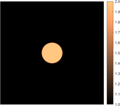
(a) Wavespeed $c$

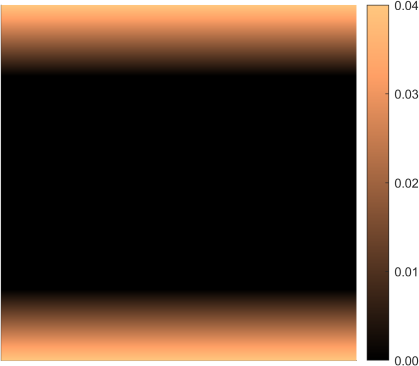
(b) Absorbing sponge $\beta$

Figure 1: (a) Wavespeed profile with an inclusion defined by (46) and (b) absorbing sponge defined by (48) to mitigate effects of the top and bottom boundaries.

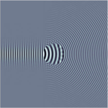
(a) Real part of one-way solution

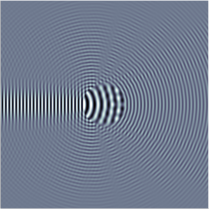
(b) Real part of two-way solution

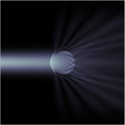
(c) Amplitude of one-way solution

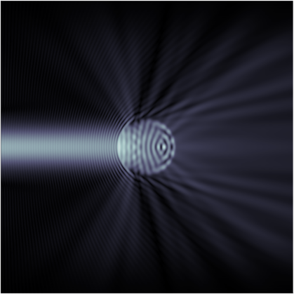
(d) Amplitude of two-way solution

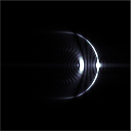
(e) FFT of one-way solution

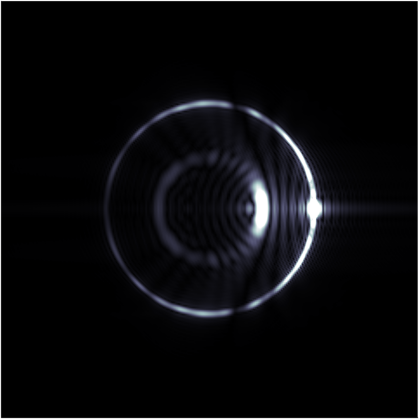
(f) FFT of two-way solution

Figure 2: Comparison between the one-way and two-way numerical solutions. These solutions were computed using Padé approximations of the pseudo-differential symbols with $4$ terms. The frequency is $\omega=120\pi$ which fits $60$ wavelengths across the domain. The two-way solution captures the reflections induced by the inclusion. These reflections are visible on plot of the real part and amplitude of the solution, as well as in the Fourier transform plots.

Table 1: Numerical approximations for the relative residuals $\|r\|_{H^{-2}(\Omega)}/\|u\|_{H^{0}(\Omega)}$ for doubling the frequency $\omega$ and linearly increasing the number of Padé terms. This configuration tests the estimates (45) obtained in Section 4 for the error and residual to decrease as $1/\omega$ as the frequency $\omega$ increases and the number of Padé terms grows logarithmically $\sim\log\omega$. The observed orders of decay were obtained as the slope of a straight line fitted through the numerical residuals versus frequency in the log-log space.

Padé terms	Relative residual (%)				Observed order
	$\omega=20\pi$	$\omega=40\pi$	$\omega=80\pi$	$\omega=160\pi$
$3$	$2.73$	$1.85$	$1.53$	$1.33$	$-0.34$
$4$	$2.46$	$1.30$	$0.63$	$0.33$	$-0.97$
$5$	$2.54$	$1.35$	$0.65$	$0.29$	$-1.04$
$6$	$2.54$	$1.35$	$0.64$	$0.29$	$-1.04$
	Observed order along the diagonal				$-1.07$

6 Conclusion and limitations

The Helmholtz equation is notoriously difficult to solve in part because the domains of dependence and influence of its solutions are global, i.e., the solution value at any specific point can affect and be affected by the solution at any other point. This phenomenon is due to the ability of waves to propagate over long distances. Hence, an effective solver (or preconditioner) must either account for such global behavior [24, 26] or incorporate a-priori assumptions about the direction of wave propagation. The pseudo-differential method presented here is designed to do the latter effectively. The pseudo-differential calculus allows us to incorporate the physical effects of variable media properties. These effects include:

1. Propagation and refraction modeled by the principal symbol $\lambda_{1}^{\pm}$ defined in (12).

2. Amplitude modulation modeled by the first term of the symbol $\lambda_{0}^{\pm}$ defined in (13).

3. Damping modeled by the second term of the symbol $\lambda_{0}^{\pm}$ defined in (13).

4. Fractional attenuation modeled by the symbol $\lambda_{\beta_{1}}^{\pm}$ defined in (14).

5. Reflection modeled by solving both the forward and the backward propagation equations (18)-(19).

6. Wide angle of wave propagation thanks to high order Padé approximations applied to the square root symbol appearing not only in the principal symbol (12) but also in (13) and (14).

Moreover, since the neglected pseudo-differential terms decay as the frequency $\omega$ increases, the proposed sweeping method is well-suited for biomedical applications based on high-frequency ultrasonics. The authors are in the process of developing numerical implementations of the proposed pseudo-differential methods to obtain ultrasound tomographic imaging and run high-intensity focused ultrasound simulations. As soon as meaningful results are obtained from these efforts, they will be reported in forthcoming publications.

In this work, we have included a proof-of-concept numerical implementation using Heun’s stepping method and second-order finite difference discretization for tangential derivatives. The purpose of the numerical implementation was to test the theoretical error estimates. However, we did not make a detailed analysis of numerical error due to discretization and of the computational cost. The use of higher-order stepping schemes (Runge-Kutta or exponential integrators) and efficient approximations of the tangential derivatives (spectral, finite element, or compact finite difference methods), and their computational advantages should be the subject of future studies. The interplay between the stepping scheme, the Padé approximations of the pseudo-differential symbols, and the step sizes on the $x$-axis and tangential directions has an impact on the numerical stability of the method. Hence, CFL-type conditions should be established for each scheme and grid refinement.

In general, the proposed pseudo-differential method is limited by its underlying assumptions, namely, that waves propagate along a dominant direction and that the media properties are smooth. Hence, we expect this method to be less accurate when waves encounter steep variations in material properties that induce refraction away from the initial dominant direction of propagation. Discontinuous jumps in media properties could be handled accurately by properly incorporating transmission conditions into the forward and backward sweeps. However, such approach remains to be developed and tested.

Appendix A Brief review of pseudo-differential operators

The notation in this section is self-contained and is not to be confused with the notation from the previous sections. Here we briefly introduce the definition of pseudo-differential operators and the basic properties of pseudo-differential calculus. We use [63, 27] as our references.

The first ingredient in this formulation is the Fourier transform $\mathcal{F}$ and its inverse $\mathcal{F}^{-1}$, which for an admissible function $u:\mathbb{R}^{d}\to\mathbb{C}$, are respectively given by

$$\mathcal{F}u(\xi)=\hat{u}(\xi)=(2\pi)^{-d/2}\int e^{-ix\cdot\xi}u(x)dx\qquad\text{and}\qquad\mathcal{F}^{-1}\hat{u}(x)=(2\pi)^{-d/2}\int e^{ix\cdot\xi}\hat{u}(\xi)d\xi.$$ (52)

The Fourier transform satisfies the following properties in relation to differentiation,

$$D^{\alpha}u(x)=(2\pi)^{-d/2}\int\xi^{\alpha}\hat{u}(\xi)e^{ix\cdot\xi}d\xi$$ (53)

for a multi-index $\alpha=(\alpha_{1},...,\alpha_{d})\in\mathbb{N}^{d}$ where $D^{\alpha}=D_{1}^{\alpha_{1}}\dots D_{d}^{\alpha_{d}}$ and $D_{j}=-i\partial_{x_{j}}$.

Now we define a differential operator of order $m$ with variable coefficients as follows,

$$A(x,D)=\sum_{|\alpha|\leq m}a_{\alpha}(x)D^{\alpha}$$ (54)

where $|\alpha|=\alpha_{1}+...+\alpha_{d}$ and the coefficients $a_{\alpha}(x)$ are smooth. Then we have

$$A(x,D)u(x)=(2\pi)^{-d/2}\int e^{ix\cdot\xi}a(x,\xi)\hat{u}(\xi)d\xi$$ (55)

where

$$a(x,\xi)=\sum_{|\alpha|\leq m}a_{\alpha}(x)\xi^{\alpha}\qquad\text{and}\qquad\xi^{\alpha}=\xi_{1}^{\alpha_{1}}\,\xi_{2}^{\alpha_{2}}\,...\,\xi_{d}^{\alpha_{d}}.$$ (56)

We call $a(x,\xi)$ the (full) symbol of the differential operator.

Now we use the Fourier integral representation (55) of differential operators to generalize them to a larger class known as pseudo-differential operators. Notice that for differential operators, the functions $a(x,\xi)$ are polynomial with respect to $\xi$. For pseudo-differential operators, we let these functions belong to larger sets, known as Hormander’s symbol classes defined as follows. Take $m\in\mathbb{R}$ and define the symbol class $\SS^{m}$ to consist of all $C^{\infty}$ functions $a(x,\xi)$ satisfying

$$|D_{x}^{\beta}D_{\xi}^{\alpha}a(x,\xi)|\leq C_{\alpha\beta}(1+|\xi|^{2})^{(m-|\alpha|)/2}$$ (57)

for all multi-indices $\alpha$ and $\beta$, and some constants $C_{\alpha\beta}$. Once a symbols $a(x,\xi)$ belongs to a class $\SS^{m}$, the associated operator $\text{Op}\left(a\right)$, defined by

$$\text{Op}\left(a\right)u(x)=(2\pi)^{-d/2}\int a(x,\xi)e^{ix\cdot\xi}\hat{u}(\xi)d\xi,$$ (58)

is said to be a pseudo-differential operator that belongs to $\text{Op}\left(\SS^{m}\right)$. In other words, pseudo-differential operators are defined by their symbols. The smallest possible $m$ that allows a symbol $a(x,\xi)$ to satisfy (57) is known as the order of the pseudo-differential operator. Note that by (57), when we take a derivative of a symbol $a(x,\xi)$ with respect to $\xi$, we simply obtain another pseudo-differential operator with lower order. Also note that (57) only dictates the behavior of the symbol at infinity, hence the symbol is allowed to have arbitrary profiles for small $\xi$ as long as the smoothness condition is satisfied.

Given a pseudo-differential operators $A\in\text{Op}\left(\SS^{m}\right)$, its symbol will be denoted $\text{Sym}(A)$. An important subset of pseudo-differential operators are those that satisfy the following conditions. Writing $a(x,\xi)=\text{Sym}(A)\in\SS^{m}$, if there are smooth $a_{m-j}(x,\xi)$ homogeneous in $\xi$ of degree $m-j$, i.e., $a_{m-j}(x,r\xi)=r^{m-j}a_{m-j}(x,\xi)$ for any $r$ and $\xi\neq 0$, and if

$$\left(a(x,\xi)-\sum_{j=0}^{J}a_{m-j}(x,\xi)\right)\in\SS^{m-J-1}\qquad\text{for all $J=0,1,2,...$,}$$ (59)

we say that $A$ is a “classical” pseudo-differential operator. In such cases when $A$ is classical, we may write

$$a\sim\sum_{j=0}^{\infty}a_{m-j},$$ (60)

and say that $\sum_{j=0}^{\infty}a_{m-j}$ is an asymptotic sum of $a$.

Finally, given two symbols $a(x,\xi)\in\SS^{m_{1}}$ and $b(x,\xi)\in\SS^{m_{2}}$, the composition of their respective operators has a symbol in $\SS^{m_{1}+m_{2}}$ and such that

$$\text{Sym}\left(\text{Op}\left(a\right)\text{Op}\left(b\right)\right)\sim\sum_{\alpha\geq 0}\frac{i^{|\alpha|}}{\alpha!}D^{\alpha}_{\xi}a(x,\xi)D^{\alpha}_{x}b(x,\xi).$$ (61)

In particular, the operator associated with the product of two symbols $a$ and $b$ satisfies,

$$\text{Op}\left(ab\right)=\text{Op}\left(a\right)\text{Op}\left(b\right)-\sum_{\alpha\geq 1}\frac{i^{|\alpha|}}{\alpha!}\text{Op}\left(D^{\alpha}_{\xi}a(x,\xi)D^{\alpha}_{x}b(x,\xi)\right).$$ (62)

Hence if $a=a(x)$ is independent of $\xi$ or $b=b(\xi)$ is independent of $x$, then $\text{Op}\left(ab\right)=\text{Op}\left(a\right)\text{Op}\left(b\right)$.

Another interesting case is the computation of the operator of a symbol of the form $1/b$ for $b\neq 0$ and $b\in\SS^{m}$. This is a special case of the above equations. So we have

$$\text{Op}\left(b\right)\text{Op}\left(1/b\right)=\text{Op}\left(1\right)+\sum_{\alpha\geq 1}\frac{i^{|\alpha|}}{\alpha!}\text{Op}\left(D^{\alpha}_{\xi}b(x,\xi)D^{\alpha}_{x}b^{-1}(x,\xi)\right).$$ (63)

Hence, provided that $\text{Op}\left(b\right)$ is invertible, then

$$\text{Op}\left(1/b\right)=\text{Op}\left(b\right)^{-1}\left(I+\sum_{\alpha\geq 1}\frac{i^{|\alpha|}}{\alpha!}\text{Op}\left(D^{\alpha}_{\xi}b(x,\xi)D^{\alpha}_{x}b^{-1}(x,\xi)\right)\right).$$ (64)

Finally, given a pseudo-differential symbol $a\in\SS^{m}$, the Sobolev norms satisfy

$$\|\text{Op}\left(a\right)u\|^{2}_{H^{s}(\mathbb{R}^{d})} \leq\int(1+|\xi|^{2})^{s}\sup_{x}{|a(x,\xi)|^{2}}|\hat{u}(\xi)|^{2}d\xi$$

$$\leq C_{00}\int(1+|\xi|^{2})^{s+m}|\hat{u}(\xi)|^{2}d\xi$$

$$=C_{00}\|u\|^{2}_{H^{s+m}(\mathbb{R}^{d})}$$ (65)

provided that $u\in H^{s+m}(\mathbb{R}^{d})$ and where $C_{00}>0$ is the constant appearing in (57). In other words, $\text{Op}\left(a\right)$ maps $H^{s+m}(\mathbb{R}^{d})$ continuously into $H^{s}(\mathbb{R}^{d})$ for any $s\in\mathbb{R}$. Moreover, the norm of $\text{Op}\left(a\right)$ is proportional to the bound on its symbol.

Appendix B Padé approximations

The real-valued Padé approximant for the function $(1+z)^{\gamma}$, as a partial fraction expansion, has the following form,

$$P_{M}(z)=a_{0}+\sum_{m=1}^{M}\frac{a_{m}}{z-b_{m}}$$ (66)

where the real-valued coefficients $a_{m}$ and $b_{m}$ are computed in order to match the value of the function $(1+z)^{\gamma}$ and its first $2M$ derivatives at $z=0$ [15]. Unfortunately, these Padé approximants suffer from inaccuracies and instabilities when $z\leq-1$ due to the branch cut along the negative real line starting at $z=-1$ [45, 46, 49, 50]. In order to avoid this problem (for the specific case of $\gamma=1/2$) Milinazzo et al. [49] considered the Padé approximation of the function $e^{i\theta\gamma}\left(1+\zeta\right)^{\gamma}$ where $\zeta=(1+z)e^{-i\theta}-1$, which has a rotated branch cut defined by the angle $\theta$. As a result, the approximation remains stable and continuous for $z\in\mathbb{R}$. This $\theta$-rotated Padé approximant of order $M$, in partial fraction form, is given by

$$P_{M,\theta}(z)=e^{i\theta\gamma}\left(a_{0}+\sum_{m=1}^{M}\frac{a_{m}}{(1+z)e^{-i\theta}-1-b_{m}}\right)=\tilde{a}_{0}+\sum_{m=1}^{M}\frac{\tilde{a}_{m}}{z-\tilde{b}_{m}}$$ (67)

where the complex-valued Padé coefficients are defined by $\tilde{a}_{0}=a_{0}e^{i\theta\gamma}$, $\tilde{a}_{m}=a_{m}e^{i\theta(1+\gamma)}$ and $\tilde{b}_{m}=(1+b_{m})e^{i\theta}-1$ for $m=1,2,...,M$ [15, 49]. In Section 3, there is need to apply the Padé method for the cases $\gamma=\pm 1/2$ to approximate the symbols $(\lambda_{1}^{+})^{\pm 1}$, and the cases $\gamma=\pm 1/4$ for the symbols $(\lambda_{1}^{+})^{\pm 1/2}$. For these cases, the real-valued Padé coefficients, displayed on Tables 2-5, were computed using Sanguigno’s MATLAB pade function to obtain a rational approximation [56], followed by R2020b MATLAB’s residue function to re-cast it as a partial fraction expansion. The well-known error analysis for Padé approximants (see for instance [15]) shows that

$$(1+z)^{\gamma}=P_{M,\theta}(z)+\mathcal{O}\left(|z|^{2M+1}\right)$$ (68)

as $z\to 0$, which justifies the error terms specified in Section 3 by replacing $z=-c^{2}\delta^{2}$.

Table 2: Real-valued Padé coefficients to approximate the function $(1+z)^{1/2}$ in partial fraction form (66) for orders $M=1,2,3,4$.

M	$a_{0}$	$a_{1}$	$a_{2}$	$a_{3}$	$a_{4}$	$b_{1}$	$b_{2}$	$b_{3}$	$b_{4}$
1	2.8889	-7.1358				-3.7778
2	4.7738	-34.5138	-0.2786			-9.6264	-1.4778
3	6.7228	-98.1129	-1.0233	-0.0723		-18.7042	-2.4499	-1.2139
4	8.6939	-213.677	-2.4055	-0.2410	-0.0303	-31.0166	-3.8025	-1.6590	-1.1242

Table 3: Real-valued Padé coefficients to approximate the function $(1+z)^{-1/2}$ in partial fraction form (66) for orders $M=1,2,3,4$.

M	$a_{0}$	$a_{1}$	$a_{2}$	$a_{3}$	$a_{4}$	$b_{1}$	$b_{2}$	$b_{3}$	$b_{4}$
1	0.3590	0.8218				-1.2821
2	0.2114	1.0955	0.4181			-2.6945	-1.0944
3	0.1493	1.4521	0.4474	0.2885		-4.9532	-1.5846	-1.0480
4	0.1152	1.8313	0.5184	0.2862	0.2219	-8.0266	-2.3254	-1.3120	-1.0292

Table 4: Real-valued Padé coefficients to approximate the function $(1+z)^{1/4}$ in partial fraction form (66) for orders $M=1,2,3,4$.

M	$a_{0}$	$a_{1}$	$a_{2}$	$a_{3}$	$a_{4}$	$b_{1}$	$b_{2}$	$b_{3}$	$b_{4}$
1	1.6239	-1.5572				-2.4957
2	2.0906	-5.8925	-0.1638			-6.0834	-1.3433
3	2.4805	-14.0723	-0.4809	-0.0572		-11.6531	-2.1510	-1.1613
4	2.8202	-26.8939	-0.9694	-0.1539	-0.0284	-19.2030	-3.2899	-1.5524	-1.0952

Table 5: Real-valued Padé coefficients to approximate the function $(1+z)^{-1/4}$ in partial fraction form (66) for orders $M=1,2,3,4$.

M	$a_{0}$	$a_{1}$	$a_{2}$	$a_{3}$	$a_{4}$	$b_{1}$	$b_{2}$	$b_{3}$	$b_{4}$
1	0.6213	0.5737				-1.5149
2	0.4794	1.1826	0.1945			-3.3516	-1.1593
3	0.4035	1.9393	0.3201	0.1095		-6.2432	-1.7354	-1.0796
4	0.3547	2.8260	0.4555	0.1670	0.0734	-10.1697	-2.5810	-1.3816	-1.0481

Appendix C Continuity estimates for the Helmholtz equation

Let $\Omega=\{(x,x_{\perp})\in\mathbb{R}^{d}:x>0,x_{\perp}\in\mathbb{R}^{d-1}\}$, the half-space, and consider the following boundary value problem for the Helmholtz operator $\mathcal{H}=\Delta+\left(\omega^{2}c^{-2}+i\omega a-a_{\alpha}(-i\omega)^{\alpha}\right)$:

$$\mathcal{H}u=f\quad\text{in}\quad\Omega,\quad u=0\quad\text{on}\quad\partial\Omega,$$ (69)

satisfying the Sommerfeld radiation condition at infinity, and where $c(x,x_{\perp})\geq c_{0}>0$, $a(x,x_{\perp})\geq a_{0}>0$ and $a_{\alpha}(x,x_{\perp})\geq 0$ are smooth functions. Here it is assumed that $c=c_{0}$, $a=a_{0}$, $a_{\alpha}=0$, and $f=0$ outside of a bounded subdomain of $\Omega$. The existence, uniqueness, and regularity of solutions for this problem can be established (in strong and weak formulations) through the method of images, ie., by extending $c$, $a$, and $a_{\alpha}$ symmetrically about $\{x=0\}$, and $f$ anti-symmetrically about $\{x=0\}$. Thus, by posing the problem in the whole-space $\mathbb{R}^{d}$, the classical results for well-posedness can be invoked [48, 21, 43]. Adding to the well-posedness, we now review the behavior of the solution with respect to the frequency $\omega$.

Theorem 1.

There is a constants $C>0$ independent of $\omega$, such that for all $f\in L^{2}(\Omega)$

$$\|u\|_{H^{2}(\Omega)}+\omega^{1/2}\|u\|_{H^{1}(\Omega)}+\omega\|u\|_{L^{2}(\Omega)}\leq C\|f\|_{L^{2}(\Omega)}$$ (70)

where $u$ is a solution to (69). The same holds for the (formal) adjoint $\mathcal{H}^{*}$.

Proof.

Elliptic regularity and the exponential decay of the solution for non-vanishing damping ($a\geq a_{0}>0$) allows us to multiply the Helmholtz equation by $\bar{u}$ and integrate on $\Omega$, obtaining

$$-\|\nabla u\|^{2}_{L^{2}(\Omega)}+\omega^{2}\|c^{-1}u\|^{2}_{L^{2}(\Omega)}+i\omega\|\sqrt{a}u\|^{2}_{L^{2}(\Omega)}-(-i\omega)^{\alpha}\|\sqrt{a_{\alpha}}u\|^{2}_{L^{2}(\Omega)}=\int_{\Omega}fu\,dx$$ (71)

From the imaginary part of the previous equality, we deduce $\|u\|^{2}_{L^{2}(\Omega)}\lesssim\omega^{-1}\|f\|_{L^{2}(\Omega)}\|u\|_{L^{2}(\Omega)}$ for $\omega$ large enough, therefore,

$$\|u\|_{L^{2}(\Omega)}\lesssim\omega^{-1}\|f\|_{L^{2}(\Omega)}.$$ (72)

On the other hand, the real part of the equality implies $\|\nabla u\|^{2}_{L^{2}(\Omega)}\leq\omega^{2}\|u\|^{2}_{L^{2}(\Omega)}+\|f\|_{L^{2}(\Omega)}\|u\|_{L^{2}(\Omega)}$, which combined with the previous inequality gives

$$\|u\|_{H^{1}(\Omega)}\leq C\|f\|_{L^{2}(\Omega)}$$ (73)

for an $\omega$-independent constant $C>0$.

A standard argument based on finite quotients and the previous inequality (see, for instance, [25]) leads to the improved regularity estimate

$$\|u\|_{H^{2}(\Omega)}\leq C\|f\|_{L^{2}(\Omega)},$$ (74)

for another constant $C>0$ independent of $\omega$. The proof concludes from the previous and interpolation inequalities. ∎

Corollary 1.

There is another constant $C>0$ independent of $\omega$ such that, for all $f\in H^{-2}(\Omega)$,

$$\|u\|_{L^{2}(\Omega)}\leq C\|f\|_{H^{-2}(\Omega)}$$ (75)

with $u$ a solution (by transposition) of (69).

Proof.

By definition, $u$ satisfies

$$\langle u,\mathcal{H}^{*}\phi\rangle=\langle f,\phi\rangle$$ (76)

for all $\phi\in H^{2}(\Omega)\cap H^{1}_{0}(\Omega)$. For an arbitrary $\psi\in L^{2}(\Omega)$ we take $\phi$ solution to $\mathcal{H}^{*}\phi=\psi$ with boundary condition $\phi=0$ as in the previous theorem. Then,

$$|\langle u,\psi\rangle|\leq\|f\|_{H^{-2}(\Omega)}\|\phi\|_{H^{2}(\Omega)}\leq C\|f\|_{H^{-2}(\Omega)}\|\psi\|_{L^{2}(\Omega)},$$ (77)

for the same constant $C>0$ from Theorem 1, which renders the desired inequality. ∎

References

- [1] S. Acosta. On-surface radiation condition for multiple scattering of waves. Comput. Methods Appl. Mech. Eng., 283:1296–1309, 2015.
- [2] S. Acosta. High order surface radiation conditions for time-harmonic waves in exterior domains. Comput. Methods Appl. Mech. Eng., 322:296–310, 2017.
- [3] S. Acosta. Local on-surface radiation condition for multiple scattering of waves from convex obstacles. Comput. Methods Appl. Mech. Eng., 378:113697, 2021.
- [4] S. Acosta and C. Montalto. Photoacoustic imaging taking into account thermodynamic attenuation. Inverse Probl., 32(11):115001, 2016.
- [5] S. Acosta and B. Palacios. Thermoacoustic tomography for an integro-differential wave equation modeling attenuation. J. Differ. Equ., 264(3):1984–2010, 2018.
- [6] S. Acosta and V. Villamizar. Coupling of Dirichlet-to-Neumann boundary condition and finite difference methods in curvilinear coordinates for multiple scattering. J. Comput. Phys., 229(15):5498–5517, 2010.
- [7] S. Acosta, V. Villamizar, and B. Malone. The DtN nonreflecting boundary condition for multiple scattering problems in the half-plane. Comput. Methods Appl. Mech. Eng., 217-220:1–11, 2012.
- [8] H. Ammari. An Introduction to Mathematics of Emerging Biomedical Imaging. Springer-Verlag, Berlin, 2008.
- [9] H. Ammari, editor. Mathematical modeling in biomedical imaging I, volume 1983 of Lecture Notes in Mathematics. Springer-Verlag Berlin Heidelberg, 2009.
- [10] H. Ammari, editor. Mathematical modeling in biomedical imaging II, volume 2035 of Lecture Notes in Mathematics. Springer-Verlag Berlin Heidelberg, 2012.
- [11] D. A. Angus. The one-way wave equation: A full-waveform tool for modeling seismic body wave phenomena. Surv. Geophys., 35(2):359–393, 2014.
- [12] X. Antoine and H. Barucq. Microlocal diagonalization of strictly hyperbolic pseudodifferential systems and application to the design of radiation conditions in Electromagnetism. SIAM J. Appl. Math., 61(6):1877–1905, 2001.
- [13] X. Antoine, H. Barucq, and A. Bendali. Bayliss-Turkel-like radiation conditions on surfaces of arbitrary shape. J. Math. Anal. Appl., 229:184–211, 1999.
- [14] J.-F. Aubry, O. Bates, C. Boehm, K. Butts Pauly, D. Christensen, C. Cueto, P. Gélat, L. Guasch, J. Jaros, Y. Jing, R. Jones, N. Li, P. Marty, H. Montanaro, E. Neufeld, S. Pichardo, G. Pinton, A. Pulkkinen, A. Stanziola, A. Thielscher, B. Treeby, and E. van’t Wout. Benchmark problems for transcranial ultrasound simulation: Intercomparison of compressional wave models. J. Acoust. Soc. Am., 152(2):1003–1019, 2022.
- [15] G. Baker Jr. and P. Graves-Morris. Pade Approximants. Encyclopedia of Mathematics and It’s Applications, Vol. 59. Cambridge University Press, second edition, 1996.
- [16] A. Bamberger, B. Engquist, L. Halpern, and P. Joly. Higher order paraxial wave equation approximations in heterogeneous media. SIAM, 48(1):129–154, 1988.
- [17] A. Bamberger, B. Engquist, L. Halpern, and P. Joly. Parabolic wave equation approximations in heterogeneous media. SIAM J. Appl. Math., 48(1):99–128, 1988.
- [18] P. Beard. Biomedical photoacoustic imaging. Interface Focus, 1:602–31, 2011.
- [19] J. Chazarain and A. Piriou. Introduction to the theory of linear partial differential equations. Studies in Mathematics and its Applications vol. 14. Elsevier, 1982.
- [20] W. Chen, S. Hu, and W. Cai. A causal fractional derivative model for acoustic wave propagation in lossy media. Arch. Appl. Mech., 86(3):529–539, 2016.
- [21] D. Colton and R. Kress. Inverse Acoustic and Electromagnetic Scattering Theory. Applied Mathematical Sciences. Springer, New York, NY, 3rd edition, 2013.
- [22] B. Engquist, A. Fokas, E. Hairer, and A. Iserles, editors. Highly Oscillatory Problems. London Mathematical Society, Lecture Note Series 366. Cambridge Univ. Press, 2009.
- [23] B. Engquist and O. Runborg. Computational high frequency wave propagation. Acta Numer., 12(2003):181–266, 2003.
- [24] O. G. Ernst and M. J. Gander. Why it is difficult to solve Helmholtz problems with classical iterative methods. Lect. Notes Comput. Sci. Eng., 83:325–363, 2012.
- [25] D. Evans, P. Lawford, J. Gunn, D. Walker, D. Hose, R. Smallwood, B. Chopard, M. Krafczyk, J. Bernsdorf, and A. Hoekstra. The application of multiscale modelling to the process of development and prevention of stenosis in a stented coronary artery. Philos. Trans. A. Math. Phys. Eng. Sci., 366(July):3343–3360, 2008.
- [26] M. J. Gander and H. Zhang. A class of iterative solvers for the Helmholtz equation: Factorizations, sweeping preconditioners, source transfer, single layer potentials, polarized traces, and optimized Schwarz methods. SIAM Rev., 61(1):3–76, 2019.
- [27] Alain Grigis and Johannes Sjöstrand. Microlocal Analysis for Differential Operators: An Introduction. London Mathematical Society Lecture Note Series vol 196. Cambridge University Press, Cambridge, 1994.
- [28] J. Gu and Y. Jing. Numerical modeling of ultrasound propagation in weakly heterogeneous media using a mixed-domain method. IEEE Trans. Ultrason. Ferroelectr. Freq. Control, 65(7):1258–1267, 2018.
- [29] J. Gu and Y. Jing. Simulation of the second-harmonic ultrasound field in heterogeneous soft tissue using a mixed-domain method. IEEE Trans. Ultrason. Ferroelectr. Freq. Control, 66(4):669–675, 2019.
- [30] L. Guasch, O. Calderon Agudo, M.-X. Tang, P. Nachev, and M. Warner. Full-waveform inversion imaging of the human brain. NPJ Digit. Med., 3(1):1–12, 2020.
- [31] K. Guo, S. Acosta, and J. Chan. A weight-adjusted discontinuous Galerkin method for wave propagation in coupled elastic-acoustic media. J. Comput. Phys., 418:109632, 2020.
- [32] L. Halpern and L. Trefethen. Wide-angle one-way wave equations. J. Acoust. Soc. Am., 84(4):1397–1404, 1988.
- [33] S. R. Haqshenas, P. Gélat, E. van ’t Wout, T. Betcke, and N. Saffari. A fast full-wave solver for calculating ultrasound propagation in the body. Ultrasonics, 110(May 2020):106240, 2021.
- [34] S. Holm and S. Nasholm. A causal and fractional all-frequency wave equation for lossy media. J. Acoust. Soc. Am., 130(4):2195, 2011.
- [35] C. Huang, L. Nie, R. Schoonover, L. V. Wang, and M. Anastasio. Photoacoustic computed tomography correcting for heterogeneity and attenuation. J. Biomed. Opt., 17(6):061211, 2012.
- [36] Y. Jing, M. Tao, and G. Clement. Evaluation of a wave-vector-frequency-domain method for nonlinear wave propagation. J. Acoust. Soc. Am., 129(1):32–46, 2011.
- [37] T. Khajah and V. Villamizar. Highly accurate acoustic scattering: Isogeometric analysis coupled with local high order farfield expansion ABC. Comput. Methods Appl. Mech. Eng., 349:477–498, 2019.
- [38] R. Kowar and O. Scherzer. Photoacoustic Imaging Taking into Account Attenuation. In Math. Model. Biomed. Imaging II, pages 85–130. Springer, 2011.
- [39] S. Leung, T. Webb, R. Bitton, P. Ghanouni, and K. Butts Pauly. A rapid beam simulation framework for transcranial focused ultrasound. Sci. Rep., 9(1):1–11, 2019.
- [40] F. Li, U. Villa, N. Duric, and M. Anastasio. A forward model incorporating elevation-focused transducer properties for 3D full-waveform inversion in ultrasound computed tomography. arXiv, 2023.
- [41] F. Li, U. Villa, N. Duric, and M. Anastasio. Three-dimensional time-domain full-waveform inversion for ring-array-based ultrasound computed tomography. J. Acoust. Soc. Am., 153(3_supplement):A353, 2023.
- [42] S. Li, M. Jackowski, D. Dione, T. Varslot, L. Staib, and K. Mueller. Refraction corrected transmission ultrasound computed tomography for application in breast imaging. Med. Phys., 37(5):2233–2246, 2010.
- [43] J.-L. Lions and E. Magenes. Non-homogeneous boundary value problems and applications, volume I of Grundlehren der mathematischen Wissenschaften in Einzeldarstellungen, Bd. 181-183. Berlin, New York, Springer-Verlag, 1972.
- [44] Y. Lou, W. Zhou, T. Matthews, C. Appleton, and M. Anastasio. Generation of anatomically realistic numerical phantoms for photoacoustic and ultrasonic breast imaging. J. Biomed. Opt., 22(4):041015, 2017.
- [45] Y. Y. Lu. A complex coefficient rational approximation of sqrt 1 + x. Appl. Numer. Math., 27:141–154, 1998.
- [46] Y. Y. Lu. A Padé approximation method for square roots of symmetric positive definite matrices. SIAM J. Matrix Anal. Appl., 19(3):833–845, 1998.
- [47] A. Malcolm and M. De Hoop. A method for inverse scattering based on the generalized Bremmer coupling series. Inverse Probl., 21(3):1137–1167, 2005.
- [48] W. McLean. Strongly Elliptic Systems and Boundary Integral Equations. Cambridge Univ. Press, 2000.
- [49] F. Milinazzo, C. Zala, and G. Brooke. Rational square-root approximations for parabolic equation algorithms. J. Acoust. Soc. Am., 101(2):760–766, 1997.
- [50] A. Modave, C. Geuzaine, and X. Antoine. Corner treatments for high-order local absorbing boundary conditions in high-frequency acoustic scattering. J. Comput. Phys., 401:109029, 2020.
- [51] S. Nasholm and S. Holm. Linking multiple relaxation, power-law attenuation, and fractional wave equations. J. Acoust. Soc. Am., 130(5):3038–3045, 2011.
- [52] L. Nirenberg. Pseudodifferential operators and some applications. In CBMS Reg. Conf. Ser. Math. AMS, volume 17, pages 19–58, 1973.
- [53] K. Opielinski and T. Gudra. Ultrasound transmission tomography image distortions caused by the refraction effect. Ultrasonics, 38(1):424–429, 2000.
- [54] T. J.P.M. Op’t Root and C. C. Stolk. One-way wave propagation with amplitude based on pseudo-differential operators. Wave Motion, 47(2):67–84, 2010.
- [55] J. Poudel, Y. Lou, and M. Anastasio. A survey of computational frameworks for solving the acoustic inverse problem in three-dimensional photoacoustic computed tomography. Phys. Med. Biol., 64(14):14TR01, 2019.
- [56] L. Sanguigno. Pade Approximant, 2023.
- [57] H. Shehadeh, A. Malcolm, and J. Schotland. Inversion of the Bremmer series. J. Comput. Math., 35(5):586–599, 2017.
- [58] Matthew P. Shortell, Marwan A.M. Althomali, Marie Luise Wille, and Christian M. Langton. Combining ultrasound pulse-echo and transmission computed tomography for quantitative imaging the cortical shell of long-bone replicas. Front. Mater., 4(November):1–8, 2017.
- [59] G. Soldati. Biomedical applications of ultrasound. In Compr. Biomed. Phys., volume 2, pages 401–436. Elsevier B.V., 2014.
- [60] C. Stolk. A pseudodifferential equation with damping for one-way wave propagation in inhomogeneous acoustic media. Wave Motion, 40(2):111–121, 2004.
- [61] C. Stolk. An improved sweeping domain decomposition preconditioner for the Helmholtz equation. Adv. Comput. Math., 43:45–76, 2017.
- [62] N. Tanushev, B. Engquist, and R. Tsai. Gaussian beam decomposition of high frequency wave fields. J. Comput. Phys., 228(23):8856–8871, 2009.
- [63] M. E. Taylor. Pseudodifferential Operators and Nonlinear PDE. Progress in Mathematics vol 100. Birkhäuser, Boston, 1991.
- [64] M. E. Taylor. Pseudodifferential Operators. In Partial Differ. Equations II Qual. Stud. Linear Equations, pages 1–73. Springer New York, 1996.
- [65] M. E. Taylor. Tools for PDE: pseudodifferential operators, paradifferential operators, and layer potentials. Mathematical Surveys and Monographs vol. 81. AMS, 2000.
- [66] B. Treeby and B. Cox. Modeling power law absorption and dispersion for acoustic propagation using the fractional Laplacian. J. Acoust. Soc. Am., 127(5):2741–48, 2010.
- [67] T. Varslot and G. Taraldsen. Computer simulation of forward wave propagation in soft tissue. IEEE Trans. Ultrason. Ferroelectr. Freq. Control, 52(9):1473–1482, 2005.
- [68] M.D. Verweij, B.E. Treeby, K.W.A. van Dongen, and L. Demi. Simulation of Ultrasound Fields. Elsevier B.V., 2014.
- [69] V. Villamizar, S. Acosta, and B. Dastrup. High order local absorbing boundary conditions for acoustic waves in terms of farfield expansions. J. Comput. Phys., 333:331–351, 2017.
- [70] V. Villamizar, D. Grundvig, O. Rojas, and S. Acosta. High order methods for acoustic scattering: Coupling farfield expansions ABC with deferred-correction methods. Wave Motion, 95:102529, 2020.
- [71] A. Webb. Introduction to Biomedical Imaging. John Wiley, Hoboken, NJ, 2003.
- [72] J. Wiskin, D. T. Borup, S. A. Johnson, and M. Berggren. Non-linear inverse scattering: High resolution quantitative breast tissue tomography. J. Acoust. Soc. Am., 131(5):3802–3813, 2012.