ProSGNeRF: Progressive Dynamic Neural Scene Graph with Frequency Modulated Auto-Encoder in Urban Scenes

Abstract

Implicit neural representation has demonstrated promising results in view synthesis for large and complex scenes. However, existing approaches either fail to capture the fast-moving objects or need to build the scene graph without camera ego-motions, leading to low-quality synthesized views of the scene. We aim to jointly solve the view synthesis problem of large-scale urban scenes and fast-moving vehicles, which is more practical and challenging. To this end, we first leverage a graph structure to learn the local scene representations of dynamic objects and the background. Then, we design a progressive scheme that dynamically allocates a new local scene graph trained with frames within a temporal window, allowing us to scale up the representation to an arbitrarily large scene. Besides, the training views of urban scenes are relatively sparse, which leads to a significant decline in reconstruction accuracy for dynamic objects. Therefore, we design a frequency auto-encoder network to encode the latent code and regularize the frequency range of objects, which can enhance the representation of dynamic objects and address the issue of sparse image inputs. Additionally, we employ lidar point projection to maintain geometry consistency in large-scale urban scenes. Experimental results demonstrate that our method achieves state-of-the-art view synthesis accuracy, object manipulation, and scene roaming ability. The code will be open-sourced upon paper acceptance.

1 Introduction

Scene reconstruction and view synthesis on urban scenes have significantly transformed our lives, particularly in navigation and autonomous driving. NeRF [14] is the most impressive method using implicit neural representation and has shown promising results for view synthesis on static and object-centric scenes. Some recent works improve the original NeRF and achieve large-scale urban scene reconstruction. Block-nerf [19] decomposes the scene into multiple blocks and enables per-block update for virtual drive-through reconstruction. Mega-nerf [20] uses expanded octree architecture for large-scale photo-realistic fly-through scenarios. Bungeenerf [24] design a growing model with residual block structure for city-level scene reconstruction.

Although existing methods have made improvements, they are still insufficient for real-world urban scenes. We summarize several core challenges for urban scene reconstruction: a) multi-dynamic objects and large-scale ego-motions. Existing algorithms have limitations in handling scenes with both complex object motions and camera movements. Their representation capabilities are also limited with their single, global scene representation for the entire scenario. b) sparse view input for dynamic objects. In real-world urban scenes, we typically have only a few viewpoints for dynamic objects, which leads to poor reconstruction performance. c) lack of annotations and labeling It is also challenging to obtain annotations and labels for real-world scenes.

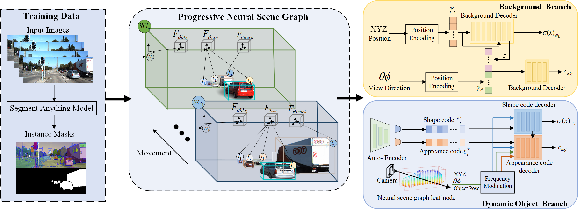
Figure 1: The isometric view of the proposed method, ProSGNeRF. We employed a 2D segmentation network, SAM, to preprocess the training data and generate accurate masks for dynamic objects. We propose a progressive neural scene graph approach that dynamically allocates local scene graph (box). The entire scene is decomposed into three parts: background, dynamic objects, and far-field. We design separate networks for background and objects and introduce a far-field loss for regularization. Nodes $l$ represent individual dynamic objects. $F_{bkg}$ models the static background scene and $F_{obj}$ models movable foreground objects in local object-centric coordinate frames.

To this end, we propose ProSGNeRF for large-scale dynamic urban scene reconstruction and novel view synthesis. For the first challenge, we utilize a neural scene graph for learning the local scene representation with decoupled object transformations and background representation. The neural scene graph incorporates a progressive scheme that employs a temporal window strategy to effectively address scalability, dividing the entire scene into multi-local scenes and dynamically initiating and maintaining local scene graphs. For the second challenge, we design a frequency auto-encoder network to encode shape and appearance features for dynamic objects and regularize the frequency range of dynamic object information, which is efficient for sparse view input and enhances the representation of dynamic objects. For the third challenge, the Segment Anything Model (SAM) has demonstrated its remarkable ability to revolutionize 2D segmentation. We leverage the promptable segmentation method to predict masks for dynamic objects and far-field scenarios, which can reduce the need for human annotation. We also use lidar projection supervision for geometry consistency. To validate our proposed framework, we evaluate the effectiveness of the method on different outdoor urban datasets, such as KITTI and VKITTI datasets [8, 3], and do exhaustive evaluations and ablation experiments on these datasets. Our system demonstrates superior performance compared to concurrent methods [16, 21] that scene reconstruction on urban scenes. In summary, our contributions are shown as follows:

• We propose a novel editable scene reconstruction method, ProSGNeRF, which decomposes dynamic, background, and far-field into a progressively neural scene graph. Our method also supports object manipulation and scene roaming.

• The proposed ProSGNeRF method processes the large-scale scenes by dynamically instantiating local neural scene graphs, enabling scalability to handle arbitrary scale scenes.

• Due to the sparse observation of objects in the urban scene, we design a frequency auto-encoder architecture network to efficiently encode shape and appearance features for the objects of interest and perform frequency modulation for sparse view inputs.

2 Related work

Recently, with the introduction and advancement of Neural Radiance Fields [14], a broad array of subsequent research has been inspired, building upon the original approach. We review the related work in the areas of implicit scene representations, dynamics, and large-scale scene representation.
Implicit Scene Representation  NeRF [14] is the most impressive work in view synthesis and 3D reconstruction. It proposes implicit representations to model scenes as functions, encoding the scene using a multi-layer perceptron (MLP). NeRF++ [26], mip-nerf [1], and mip-NeRF 360 [2] further improve the representation ability for unbounded environments. Those methods use the non-linear scene parameterization method to model unbounded scenes. NeRF-W [13] incorporate per-image embeddings to model appearance variation of the outdoor scenes.
Dynamics  There are some methods that focus on dynamic object reconstruction, such as Neural 3D Video Synthesis [10] and Space-time Neural Irradiance Fields [23]. These approaches encode time information into scene representation. [11] and [7] incorporate 2D optical flow with warping-based regularization losses to enforce multi-view consistency and dynamic object perception. Nerfies [17] and Hypernerf [18] design a per-frame deformation field for dynamic humans. These methods are limited to single-object scenes, whereas our method scales beyond synthetic and indoor scenes to urban scenes .
Large-scale Scene Representation For large-scale scene representation, [24] proposes Bungeenerf with a progressively growing model for city-level rendering. Block-NeRF [19] and Mega-NeRF [20] decompose the scene into multiple local radiance fields for large-scale scenes. However, these methods can only deal with static environments. Dynamic objects are prevalent in real-world urban road scenes. Panoptic-NeRF [6] and Panoptic Neural Fields [9] produce panoptic segmentation jointly with scene representations, achieving urban scene reconstruction.
NSG [16], SUDS [21], and Mars [22] are the most relevant works to ours. Both NSG and Mars adopts neural scene graphs and dynamic object bounding boxes to decouple the scene but cannot handle ego-motion. Besides, NSG needs over 1TB of memory to represent a 30-second video. SUDS [21] uses a large model (DINO [4]) to distill scene features and obtain semantic information and scene flow. Their methods can handle camera ego-motion and static objects but struggle with high-dynamic objects. In contrast, our approach effectively addresses large-scale camera ego-motion and dynamic objects, enabling urban scene editing useful for constructing simulators for autonomous driving.

3 Method

The pipeline of our system is shown in Fig. 1. We use a set of sequential RGB images $\{I_{i}\}_{i=1}^{M}$ with known pose $\{R|t\}$ as our input. We construct the progressive neural scene graph with the instance mask from SAM and 3D bounding box. The scene is decomposed into multi-local scene graphs with three branches: background, dynamic objects, and far-field. In the dynamic objects branch, we design a frequency auto-encoder to learn a normalized, object-centric representation whose embedding describes and disentangles shape, appearance, and pose. The decoder translates the features into occupancy and color information for given 3D points and viewing directions in object space. We also design lidar points projection geometry consistency in large-scale urban scenes.

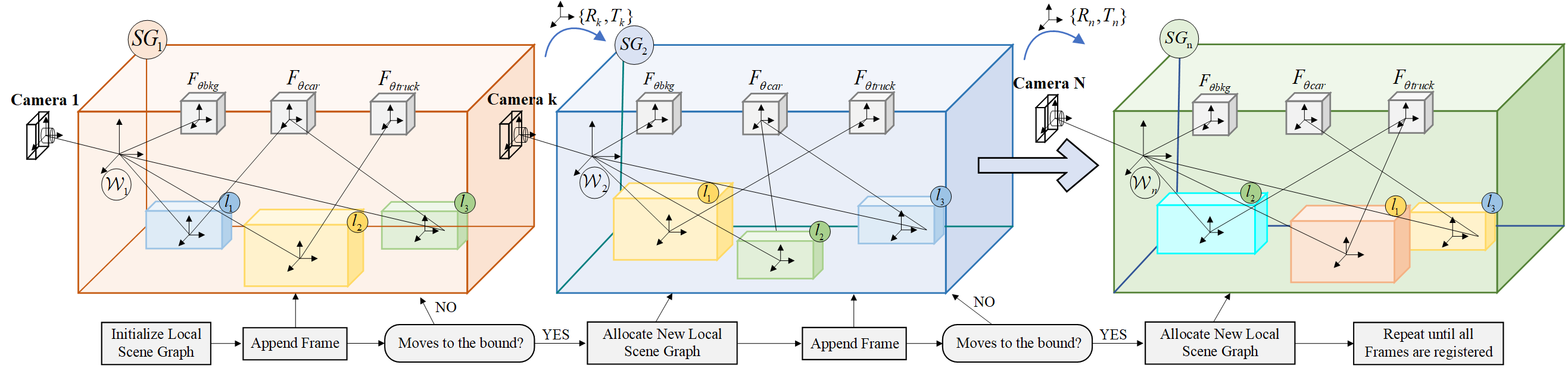
Figure 2: The isometric view of the proposed progressive neural scene graph. This scene representation uses a progressive scheme that dynamically allocates a local neural scene graph (box) based on the camera pose. Adjacent local scene graphs have overlapping regions to maintain global consistency. The leaf nodes$l$ are represented as boxes, each accompanied by their respective local Cartesian coordinate axes. We also visualize the transformations and scaling between root and leaf coordinate frames using arrows with annotated transformation and scale matrices. The overall representation model is denoted as $F_{\theta}$.

3.1 Progressive Neural Scene Graph

All the existing dynamic NeRF systems have difficulties in large-scale urban scenes. They use a single, global representation for the entire environment, which limits their scene representation capacity. It causes problems when modeling large scenes: a) a single model with fixed capacity cannot represent arbitrarily large-scale scenes. b) any misestimation has a global impact and might cause false reconstruction.

To this end, we design a progressive neural scene graph to represent city-scale scenes with multi-dynamic objects. In Figure 2, the scene graph $\mathrm{SG}$ is depicted, encompassing cameras, static nodes, and a collection of dynamic nodes. These dynamic nodes capture the evolving aspects of the scene, encapsulating the object’s appearance, shape, and various classes.

The entire scene is decomposed into several local scene representations:

$$\{I_{i},D_{i}\}_{i=1}^{M}\mapsto\{\mathrm{SG}^{1}_{\theta_{1}},\mathrm{SG}^{2}_{\theta_{2}},\dots,\mathrm{SG}^{n}_{\theta_{n}}\}\mapsto\{c,\sigma\}$$

$$\mathrm{SG}=\langle\mathcal{W},C,L,F,E\rangle$$ (1)

where the root node of scene graph denoted as $\mathcal{W}$, $C$ is a leaf node representing the camera and its intrinsic $K\in\mathbb{R}^{3\times 3}$. $L$ denotes the leaf node of scene graph(e.g. objects and background). $F$ represents the neural networks for both static and dynamic nodes: $F=F_{\theta_{bckg}}\cup\left\{F_{\theta_{1}},F_{\theta_{2}},\dots,F_{\theta_{c}}\right\}$. $E$ are edges that represent affine transformations from $i$ to $i^{\prime}$:

$$E =\left\{e_{i,i^{\prime}}\in\left\{[],\boldsymbol{T}_{i\to i^{\prime}}\right\}\right\},$$ (2)

$$\text{ with }\quad\boldsymbol{T}_{i\to i^{\prime}} =\left[\begin{array}[]{cc}\boldsymbol{R}_{i\to i^{\prime}}&\boldsymbol{t}_{i\to i^{\prime}}\\ \mathbf{0}&1\end{array}\right],$$

$$\boldsymbol{R}_{i\to i^{\prime}} \in\mathbb{R}^{3\times 3},\quad\boldsymbol{t}_{i\to i^{\prime}}\in\mathbb{R}^{3}\text{. }$$

For all edges that emanates from the root node$\mathcal{W}$, we allocate transformations that bridge the global world space and the local objects, represented by the transformation matrix $T$ We compute the scaling factor $S_{o}$, assigned at edge $e_{o}$ between an object node and its shared representation model $F$.

In our method, we dynamically create local scene representation. Whenever the estimated camera pose trajectory reaches the bound of the current scene graph, we initialize the local representation with a local subset of frames, and then we progressively introduce subsequent frames to the optimization. Each subset contains some overlapping images, essential for achieving consistent reconstructions in the global scene. We further use inverse distance weight (IDW) fusion for all overlapping scene representations. Whenever the camera pose leaves the bound of the current scene representation, we stop optimizing previous ones (freeze the network parameters). At this point, we can reduce memory requirements and clear any supervising frames that are not needed anymore.

The progressive scene graph effectively addresses the camera’s large-scale ego-motion issue. It allows our scene reconstruction to scale to arbitrary sizes, significantly enhancing our capability to represent large-scale urban scenes.

3.2 Background Model

Our local scene graph contains a background representation node, shown at the top of Fig. 1, which models the background and static objects. The static background module function maps a coordinate $x$ to its density and color:

$${[\sigma(\boldsymbol{x}),\boldsymbol{z}]} =F_{\theta_{bkg,1}}\left(\gamma_{x}(\boldsymbol{x})\right)$$ (3)

$$\boldsymbol{c}(\boldsymbol{x}) =F_{\theta_{bkg,2}}\left(\gamma_{d}(\boldsymbol{d}),\boldsymbol{z}\right)$$

We map the positional and directional inputs with $\gamma_{x}(\boldsymbol{x})$ and $\gamma_{d}(\boldsymbol{d})$ to higher frequency feature vectors to aid learning in the MLP model. There are two stages of the representation network: $F_{\theta_{bkg_{1}}}$, $F_{\theta_{bkg_{2}}}$. The output of the first MLP is the density and the latent code $z$, which encodes the geometry feature. We concatenate $z$ with the directional feature $\gamma_{d}(\boldsymbol{d})$ as the input of the second background model. Thus, the background representation is implicitly stored in the weights.

3.3 Frequency Auto-Encoder

All existing NeRF methods have difficulties in multi-dynamic objects in urban scenes. The original NeRF method assumes the density $\sigma$ is static, but both the density $\sigma(\boldsymbol{x})$ and color $\boldsymbol{c}(\boldsymbol{x})$ depend on time (and video). SUDS [21] uses an optical flow method to differentiate dynamic objects from the background. However, their method cannot model dynamic objects effectively, resulting in blurred object portions and numerous artifacts in the rendered images. Furthermore, most of the dynamic objects only appear in a few observations. This setting starkly contrasts the majority of existing works that observe multiple views of the same object. To address this challenging problem, we propose a frequency auto-encoder in dynamic objects node to learn a normalized, object-centric high-level feature that describes and disentangles shape, appearance, and pose.

Dynamic Objects Node $L_{o}$. The architecture of our dynamic branch is shown in Fig. 1. We consider each rigid part that changes its position through the observation as the dynamics. Each dynamic object is represented by the frequency auto-encoder in the local space of its node $L_{o}$ and position $p_{o}$. As the global location $p_{o}$ of a dynamic object moves between frames, its scene representation also moves. We introduce local Object Coordinate Space (OCS) $F_{o}$, fixed and aligned with the object’s pose. The transformation in the the global frame $F_{W}$ to $F_{o}$ is given by

$$\boldsymbol{x}_{o}=\boldsymbol{S}_{o}\boldsymbol{T}_{o}^{w}\boldsymbol{x}$$ (4)

where $S_{o}$ is the inverse length of the bounding box size $s_{o}=[L_{o},H_{o},W_{o}]$ with $So=diag(1/so)$. The scaling factor allows the network to learn size-independent representation. We share the weights of the network for the objects with a similar appearance and shape.

Shape and Appearance Encoder. For a input image $I$, we use the segment anything model and 3D object detector to get the 2D mask $M$ and 3D bounding box $\beta$. We encode the input images $I$ depicting a given object of interest into a shape code $\mathcal{S}_{\theta}$ and an appearance code $\mathcal{A}_{\theta}$ via a neural network. Inspired by [15], we design a two-head output architecture with the CNN feature extractor for generating the shape code $l_{s}$ and appearance code $l_{a}$, respectively.

Shape and Appearance Decoder $\phi$. The shape code $l_{s}$ is fed to the shape decoder network $\phi_{s}$ which implicitly outputs an density value $\sigma$ of the given coordinate$x$. Unlike the shape code decoder, the appearance code decoder $\phi_{a}$ uses both shape and appearance codes as the input with the positional and directional information. The appearance decoder also takes the dynamic object node information to perceive the object’s position better and implicitly outputs the RGB color $c$. Implementation details of the following encoder and decoders can be found in the supplementary material.

Frequency Modulation. In real-world urban scenes, dynamic objects only appear in a few observations, which significantly differs from the settings of the original NeRF method. In sparse view settings, the Neural radiance field is prone to overfitting to these 2D images without explaining 3D geometry in a multi-view consistent way, leading to reconstruction failure. Prior work [25] has already demonstrated that this issue is presumably caused by the high-frequency feature of the input.

To this end, we further improve the feature-extracting network with a frequency regularization method. The original auto-encoder addressed the sparsity issue by utilizing a CNN network to encode the high-frequency features, which leads to the overfitting of high-frequency features. In this work, we use a linearly increasing frequency mask $\boldsymbol{\alpha}$ to regulate the visible frequency spectrum of the position embedding function:

$$\gamma_{L}(\mathbf{x})=\left[\sin(\mathbf{x}),\cos(\mathbf{x}),\ldots,\sin\left(2^{L-1}\mathbf{x}\right),\cos\left(2^{L-1}\mathbf{x}\right)\right]$$

$$\gamma_{L}^{\prime}(t,T;\mathbf{x})=\gamma_{L}(\mathbf{x})\odot\boldsymbol{\alpha}(t,T,L)$$ (5)

where $t$ and $T$ are the current training iteration and the final iteration of frequency regularization. The mask $\boldsymbol{\alpha}$ is increased based on the training time:

$$\boldsymbol{\alpha}_{n}(t,T,L)=\begin{cases}1&\text{ if }n\leq\frac{t\cdot L}{T}+3\\ \frac{t\cdot L}{T}-\left\lfloor\frac{t\cdot L}{T}\right\rfloor&\text{ if }\frac{t\cdot L}{T}+3<n\leq\frac{t\cdot L}{T}+6\\ 0&\text{ if }n>\frac{t\cdot L}{T}+6\end{cases}$$ (6)

$\boldsymbol{\alpha}_{n}$ denotes the n-th value of $\boldsymbol{\alpha}$. Our method starts with raw inputs without positional encoding (low-frequency). Then, our mask linearly increases the visible frequency brand as training progresses. Our frequency modulation avoids the unstable and susceptible high-frequency signals of those dynamic objects at the beginning of training. We gradually provide our network with high-frequency signals to avoid over-smoothness.

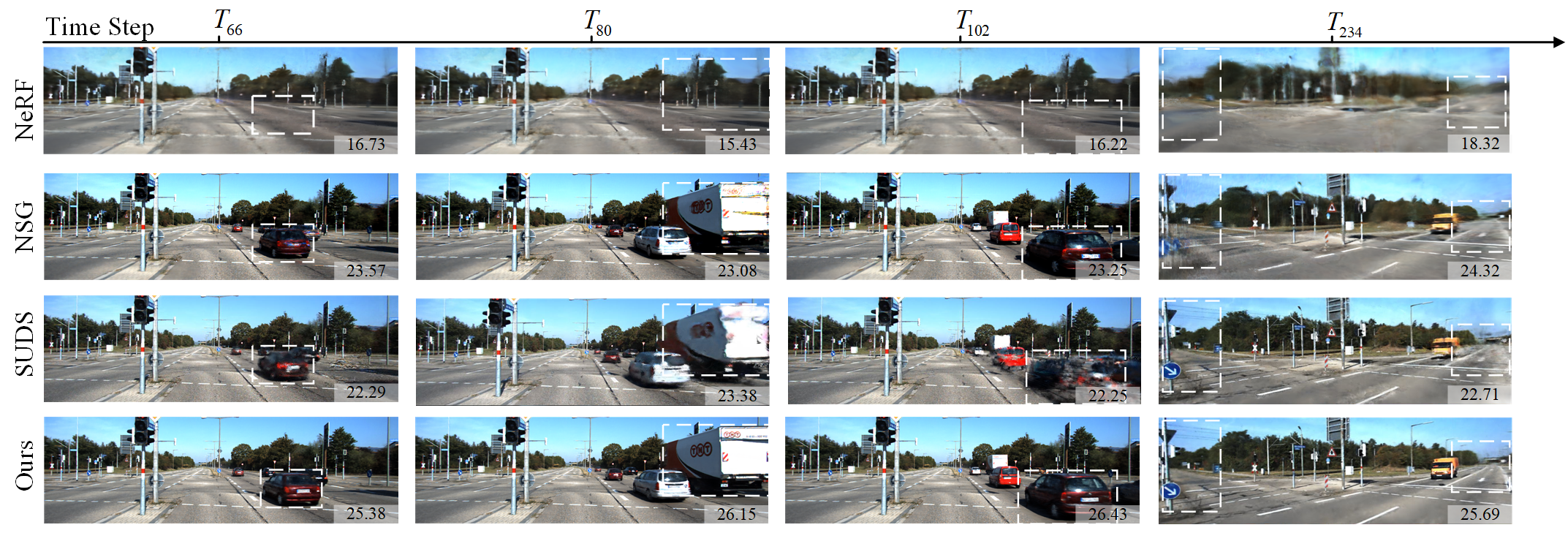
Figure 3: Qualitative results on reconstruction and novel scene arrangements of a scene from the KITTI dataset [8] for NeRF [14], NSG [16], SUDS [21] and our method. From left to right, these images correspond to different timesteps captured in the dynamic scene. We place the PSNR values of each scene in the bottom right corner. NeRF and SUDS are limited in their ability to properly represent the dynamic parts of the scene. In contrast, our neural scene graph method achieves high-quality view synthesis results for both image reconstruction and novel scene synthesis, regardless of scene dynamics.

Methods	Object Manipulation	Ego- Motion	Image Reconstruction			Novel View Synthesis
			KITTI [8]			KITTI - 75%			KITTI - 50%			KITTI - 25%
			PSNR$\uparrow$	SSIM$\uparrow$	LPIPS$\downarrow$	PSNR$\uparrow$	SSIM$\uparrow$	LPIPS$\downarrow$	PSNR$\uparrow$	SSIM$\uparrow$	LPIPS$\downarrow$	PSNR$\uparrow$	SSIM$\uparrow$	LPIPS$\downarrow$
NeRF [14]	✗	✗	18.54	0.563	0.431	18.50	0.554	0.438	18.12	0.547	0.447	17.81	0.535	0.468
NeRF$+$Time	✗	✗	23.18	0.647	0.205	20.85	0.602	0.272	21.34	0.615	0.255	18.55	0.566	0.267
NSG [16]	✓	✗	25.34	0.744	0.192	23.26	0.673	0.204	22.74	0.659	0.216	21.13	0.632	0.225
SUDS [21]	✗	✓	26.95	0.805	0.153	22.77	0.797	0.095	23.12	0.821	0.095	20.76	0.747	0.117
Ours	✓	✓	27.37	0.857	0.153	24.35	0.823	0.086	24.75	0.834	0.082	22.35	0.792	0.095

Table 1: Image reconstruction and novel view synthesis results on the complete KITTI [8] 0006 sequence. We compare our method with others on PSNR, SSIM, and LPIPS metrics. For PSNR and SSIM, higher is better; for LPIPS, lower is better. Our method generates higher-quality rendering images both in image reconstruction and novel view synthesis.

All the additional information related to scene graph dynamic objects nodes: the coordinate $\boldsymbol{x}$, direction $\theta\phi$, and object pose is embedded by our frequency encoding before they are put into the auto-encoder. Our frequency auto-encoder significantly improves the scene representation of dynamic objects and achieves great performance in image reconstruction, novel view synthesis, and object editing.

3.4 Scene Graph Rendering

This section presents the differentiable rendering of our proposed progressive neural scene graph. Each local scene graph has a subset of overlapping images $I_{k}\in\mathbb{R}^{H\times W\times 3}$. The rays are generated from the images in scene graph $SG$ with the camera intrinsic $K$ and the transformation matrix $T$. We can determine a ray $r(t)=o+td$, whose origin is at the camera center of projection $o$, and ray direction $r$.

We use different sampling strategies for the background and dynamic objects. For the background, we use a multi-plane sampling strategy to increase efficiency. We define $N_{s}$ planes parallel to the image plane of the initial camera pose $T_{wc}$. The sample planes are within the near $d_{n}$ and far planes $d_{f}$ with stratified distribution. For a ray $r$, we calculate the intersections $t_{n=1}^{N_{s}}$ with each plane and get the sample point $\boldsymbol{x}_{bkg}$ of the background.

Ray-Box Sampling. For each ray $r$ in the dynamic object node, we use the ray-box sampling method. We check the rays that intersect with the dynamic object nodes and translate them to the object coordinate space. Then, we apply the efficient AABB intersection method [12] to compute all ray-box entrance and exit points $(t_{o1},t_{oN})$. We stratified sample points $\boldsymbol{x}_{o}$ between the entrance and exit points:

$$t_{on}=\frac{n-1}{N_{d}-1}\left(t_{oN}-t_{o1}\right)+t_{o1}$$ (7)

Volume Rendering. The sample points along the rays can be represented as:$\left\{t_{i}\right\}_{i=1}^{N_{s}+m_{j}N_{d}}$. $m_{o}$ represents the number of dynamic nodes that the ray intersects along its path. The color $c(x_{i})$ and volumetric density $\sigma(x_{i})$ of each intersection point is predicted from the respective network in the static background node $F_{\theta_{bkg}}$ or dynamic objects node $F_{\theta_{o}}$. Then, we define the termination probability and color as:

$$\hat{\boldsymbol{C}}(\boldsymbol{x})=\sum_{i=1}^{N_{s}+m_{j}N_{d}}T_{i}\alpha_{i}\boldsymbol{c}_{i},\hat{\boldsymbol{D}}(\boldsymbol{x})=\sum_{i=1}^{N_{s}+m_{j}N_{d}}T_{i}\alpha_{i}\delta_{i}$$ (8)

$$T_{i}=\exp\left(-\sum_{k=1}^{i-1}\sigma_{k}\delta_{k}\right),\alpha_{i}=1-\exp\left(-\sigma_{i}\delta_{i}\right)$$ (9)

where $\delta_{i}=t_{i+1}-t_{i}$ is the distance between adjacent points.

3.5 Progressive Scene Graph Joint Learning

For the large-scale dynamic scene, we divide the entire scene into multi-local scene graphs. Whenever the camera moves to the bound of the current scene graph, we dynamically initialize a new neural scene graph and stop optimizing the previous ones. In each local scene graph, we use color loss to optimize the representation model for the background and dynamic object node:

$$\mathcal{L}_{c}=\frac{1}{N}\sum_{i=1}^{N}\left(\hat{\boldsymbol{C}}_{i}-C_{i}\right)^{2}$$ (10)

In addition, we propose a lidar points projection loss to supervise our rendering depth and enhance the geometry consistency:

$$\mathcal{L}_{d}=\frac{1}{\left|R_{i}\right|}\sum_{i\in R_{i}}\left(\hat{\boldsymbol{D}_{i}}-\Pi(P,\{R,t\},K)\right)^{2}$$ (11)

where $\Pi()$ is the projection from 3D point $P_{i}$ to the depth of 2D pixel. $R_{i}$ is the set of rays with a valid depth projection value. Inspired by [5], we also use ray distribution loss to minimize the KL divergence between the rendered ray distribution $h(t)$ and the noisy depth distribution:

$$\mathcal{L}_{\sigma}=\sum_{i}logh_{i}\mathrm{exp}(-\frac{(t_{i}-\hat{\boldsymbol{D}_{i}})^{2}}{2\hat{\sigma}_{i}^{2}})\delta_{i}$$ (12)

where $\hat{\sigma}_{i}^{2}$ is the variance of depth $D_{i}$.

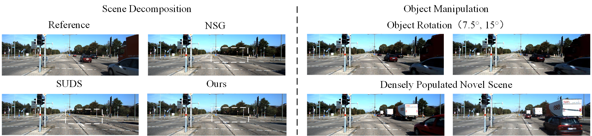
Figure 4: Scene decomposition and object manipulation. We demonstrate the decomposition capability of our progressive scene graph compared to other methods, emphasizing its capacity to isolate foreground objects and generate cleaner backgrounds. Additionally, the right part showcases our proficiency in scene editing, depicting our capability to render rotated objects and synthesize densely populated novel scenes realistically.

Methods	Image Reconstruction			Novel View Synthesis
	KITTI* [8]			KITTI* - 75%			KITTI* - 50%			KITTI* - 25%
	PSNR$\uparrow$	SSIM$\uparrow$	LPIPS$\downarrow$	PSNR$\uparrow$	SSIM$\uparrow$	LPIPS$\downarrow$	PSNR$\uparrow$	SSIM$\uparrow$	LPIPS	PSNR$\uparrow$	SSIM$\uparrow$	LPIPS$\downarrow$
NeRF [14]	16.98	0.509	0.524	16.81	0.509	0.524	16.64	0.504	0.535	16.55	0.498	0.544
NeRF + Time	24.18	0.677	0.237	22.05	0.612	0.262	21.90	0.602	0.239	20.17	0.591	0.253
NSG [16]	26.66	0.857	0.071	25.25	0.801	0.089	24.81	0.786	0.105	22.31	0.752	0.134
SUDS [21]	28.31	0.857	0.065	25.21	0.834	0.144	24.29	0.821	0.156	19.73	0.758	0.217
Ours	30.31	0.891	0.055	26.75	0.853	0.084	25.55	0.841	0.089	23.35	0.802	0.109

Table 2: We report the PSNR, SSIM, and LPIPS metrics results on the subsequent scenes from KITTI 0006 [8], following the setting of NSG and SUDS. Our approach outperforms prior methods of reconstruction and novel view synthesis across all evaluation metrics for image quality.

Far-Field Modeling (Sky). Outdoor scenes contain sky regions where rays never intersect any opaque surfaces, and thus, the NeRF model gets a weak supervisory signal in those regions.

To modulate which rays utilize the environment map, we run the segment anything model (SAM) for each image to detect pixels of the sky: $S_{i}=S(I_{i})$, where $S_{i}(r)=1$ if the ray $r$ goes through a sky pixel in image $i$. We then design a far-field loss to encourage at all point samples along rays through sky pixels to have zero density:

$$\mathcal{L}_{\mathrm{seg}}=\mathbb{E}_{\mathbf{r}\sim I_{i}}\left[\mathcal{S}_{i}(\mathbf{r})\int_{t_{n}}^{t_{f}}(T\cdot\alpha)^{2}dt\right]$$ (13)

At each step, the gradient at each trainable node in $L$ and $F$ intersecting with the rays is computed and backpropagated.

4 Experiments

In this section, we validate the proposed ProSGNeRF method on the existing automotive datasets KITTI [8] and VKITTI [3]. We validate that our method outperforms existing dynamic representation methods in image reconstruction, novel view synthesis, and dynamic object manipulation.

Datasets and Metrics. We evaluate ProSGNeRF on Kitti tracking datasets [8] for the real-world urban scene. The Kitti dataset [8] is captured using a stereo camera. Each sequence consists of more than 100 time steps and images of size $1242\times 375$, each from two camera perspectives and more than 12 dynamic objects from different classes. We also use synthetic data from the Virtual KITTI 2 Dataset [3]. We report the standard view synthesis metrics PSNR, SSIM, and LPIPS scores for all evaluations.

Implementation details and Baselines. ProSGNeRF is evaluated on a desktop PC with NVIDIA RTX 3090ti GPU. For experimental settings, the auto-encoder uses the ResNet34 backbone pre-trained on ImageNet. Each decoder uses the five fully-connected residual blocks. We set $\lambda_{c}=1$ , $\lambda_{d}=0.005$ ,$\lambda_{\sigma}=0.005$, $\lambda_{seg}=0.001$. The bounding box dimensions are scaled to include the shadows for better reconstruction. For further details of our implementation, refer to the supplementary. We compare our method against state-of-art implicit neural rendering methods: the original NeRF implementation [14], NeRF+Time, NSG [16], and SUDS [21].

4.1 Experimental Results

Image Reconstruction and Novel View Synthesis. We conduct image reconstruction and novel view synthesis experiments in urban dynamic scenes. In Tab. 1, we present our qualitative results of image reconstruction and view synthesis on KITTI datasets [8]. We evaluate the methods using different train/test splits, holding out the full dataset, every fourth time step, every other time step, and finally, training with only one in every four time steps. We present quantitative results with the PSNR, SSIM, and LPIPS metrics. The proposed method outperforms all baseline methods on all metrics. Especially as the number of training views decreases, our method demonstrates a more pronounced advantage in novel view synthesis.

The qualitative results are shown in Fig. 3. This figure depicts the appearance of the dynamic scene at different time instances from left to right (time step: 66, 80, 102, 234). The vanilla NeRF implicit rendering fails to reconstruct dynamic scenes accurately. It can only represent static scenes, which leads to nearly identical render frames for all the sequences. The NSG algorithm provides a relatively accurate representation of dynamic objects but cannot handle scenes with camera ego-motion. This limitation arises from the fixed root of their scene graph representation, which cannot move with the camera. In the last column of the figure, their reconstruction results appear highly blurred when the camera moves. SUDS exhibits poor representation capability for dynamic objects; their objects appear blurry in Fig. 1. Especially as the number of training views decreases, all the existing methods generate ghosting artifacts near areas of movement. We also present object PSNR and LPIPS curves as the training view falls in Fig. 5. ProSGNeRF achieves the best reconstruction and novel view synthesis results in dynamic object representation and large-scale camera ego-motion.

Methods	VKITTI [3]-50%
	NeRF	NeRF + Time	NSG	SUDS	Ours
PSNR$\uparrow$	18.58	18.90	23.23	23.78	27.25
SSIM$\uparrow$	0.545	0.565	0.679	0.851	0.902
LPIPS$\downarrow$	0.372	0.305	0.167	0.088	0.077

Table 3: Novel View Synthesis on VKITTI datasets [3]. We outperform past works on image reconstruction accuracy, following their experimental protocol and self-reported accuracy.

Scene Decomposition and Object Manipulation. Compared to other methods, our approach excels significantly in its ability for scene decomposition and object manipulation. The structure of the proposed method can naturally decompose scenes into dynamic and static scene components. We present the rendering of isolated nodes of our progressive scene graph in Fig. 4 to present the scene editing ability. In Fig. 4, we compared the scene decomposition ability of our method and other methods. We can see that our method learns a clean decomposition between the objects and the background.

We then generate previously unseen frames of novel object arrangements, temporal variations. Our progressive neural scene graph architecture allows dynamic urban scene editing, which can be manipulated at its edges and nodes. To exhibit the flexibility of our proposed scene representation, we manipulate the pose of dynamic objects through rotation. We present the view synthesis results in Fig. 4. Note that we have not observed the rotation of dynamic objects during training.

In addition to object manipulation and node removal of the dynamic objects, our method allows for constructing completely novel scene graphs and novel view synthesis. Fig. 4 shows view synthesis results that we randomly insert new object nodes and new object positions with new transformations. We constrain samples to the joint set of all observed road trajectories. Note that all these translations and manipulations have not been observed during training.

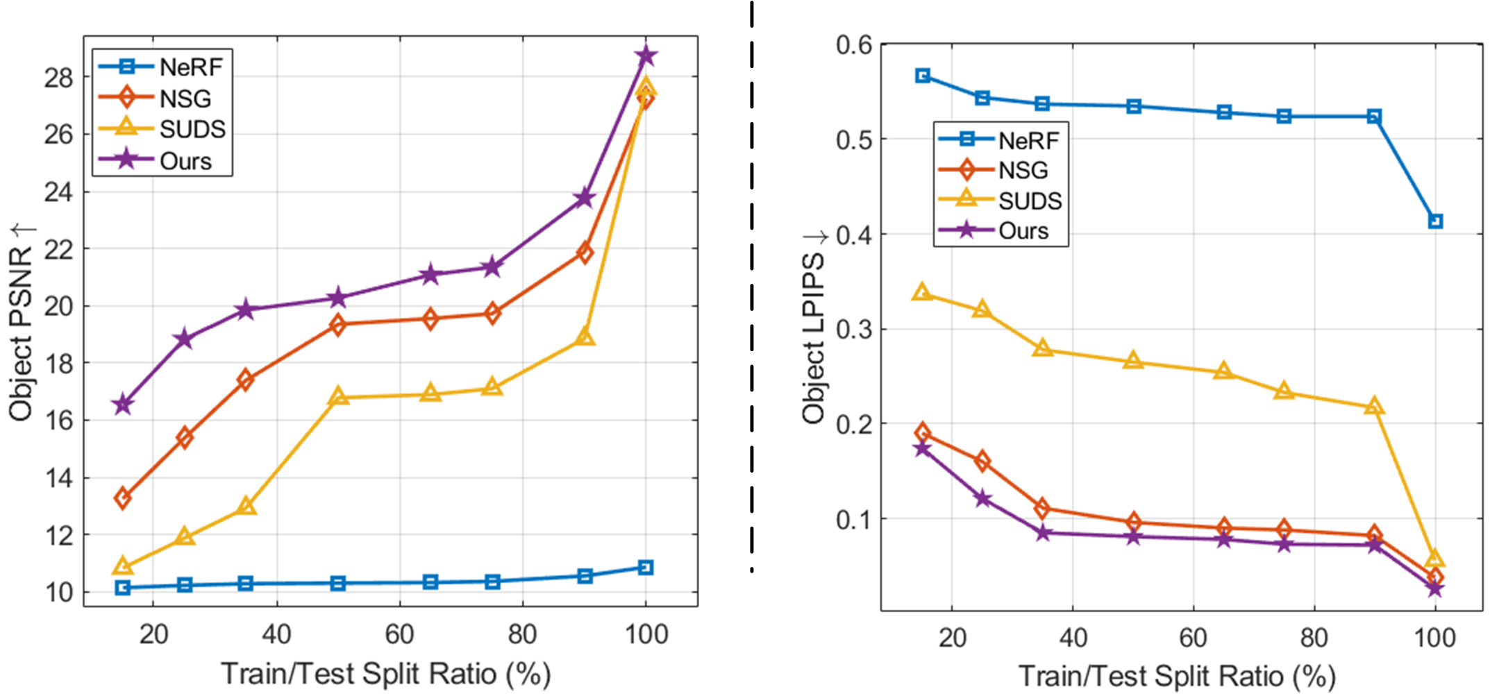
Figure 5: Dynamic objects view synthesis evaluation: measures of image fidelity plotted against train/test split ratio.

4.2 Ablation Study

We conduct an ablation study to verify the importance of the components of our method. The results of our experiments are presented in Tab. 4.

Progressive scene graph. We use the original neural scene graph instead of our progressive scene graph, which leads to a remarkable decrease in the image accuracy metrics in dynamic urban scenes with large-scale camera ego-motion.

Frequency auto-encoder. In the second experiment, we replace our frequency auto-encoder with the original MLP. We can see that the network cannot effectively represent dynamic objects due to the sparsity and movement of dynamic objects.

Loss. In the third and fourth experiments, we remove the depth loss and KL divergence loss from our network and compare it to the full model. The comparison indicates that the depth loss and KL divergence loss provide the geometry consistency of the scene representation, improving the scene’s accuracy and geometry representation. The full model achieves the best image reconstruction and novel view synthesis performance.

Methods	PSNR $\uparrow$	SSIM $\uparrow$	LPIPS $\downarrow$
w/o progressive scene graph	27.21	0.782	0.079
w/o frequency auto-encoder	28.32	0.823	0.069
w/o depth loss	28.93	0.824	0.078
w/o KL divergence loss	29.45	0.84	0.073
Full Model	30.31	0.891	0.055

Table 4: Ablation study. We conduct experiments on KITTI tracking 0006 sequence [8] to verify the effectiveness of our method. Our full model achieves the best view synthesis results.

5 Conclusion

We present the first approach that tackles the challenge of representing multi-dynamic object scenes with large-scale camera ego-motion. A progressive neural scene graph method is proposed, which learns a graph-structured and spatial representation of multiple dynamic and static scene elements. Our method dynamically instantiates local scene graphs and decomposes the entire scene into multiple local scene graphs, significantly improving the representation ability for large-scale scenes. For dynamic objects, our frequency auto-encoder network efficiently encodes shape and appearance, addressing sparse view observations through frequency modulation. Extensive experiments on both simulated and real data achieve photo-realistic quality, showcasing the effectiveness of our approach. We believe that this work opens up the field of neural rendering for city-scale dynamic scene reconstruction.

Limitations  Although we present a first attempt at building city-scale dynamic environments, many problems still need to be solved. We need the ground truth camera pose, which is challenging to get in the real-world environment.

6 Acknowledgement

Authors gratefully appreciate the contribution of Yanbo Wang from Shanghai Jiao Tong University, Zirui Wu and Yongliang Shi from Institute for AI Industry Research (AIR), Tsinghua University.

References

- [1] Jonathan T Barron, Ben Mildenhall, Matthew Tancik, Peter Hedman, Ricardo Martin-Brualla, and Pratul P Srinivasan. Mip-nerf: A multiscale representation for anti-aliasing neural radiance fields. In Proceedings of the IEEE/CVF International Conference on Computer Vision, pages 5855–5864, 2021.
- [2] Jonathan T Barron, Ben Mildenhall, Dor Verbin, Pratul P Srinivasan, and Peter Hedman. Mip-nerf 360: Unbounded anti-aliased neural radiance fields. In Proceedings of the IEEE/CVF Conference on Computer Vision and Pattern Recognition, pages 5470–5479, 2022.
- [3] Yohann Cabon, Naila Murray, and Martin Humenberger. Virtual kitti 2. arXiv preprint arXiv:2001.10773, 2020.
- [4] Mathilde Caron, Hugo Touvron, Ishan Misra, Hervé Jégou, Julien Mairal, Piotr Bojanowski, and Armand Joulin. Emerging properties in self-supervised vision transformers. In Proceedings of the IEEE/CVF international conference on computer vision, pages 9650–9660, 2021.
- [5] Kangle Deng, Andrew Liu, Jun-Yan Zhu, and Deva Ramanan. Depth-supervised nerf: Fewer views and faster training for free. In Proceedings of the IEEE/CVF Conference on Computer Vision and Pattern Recognition (CVPR), pages 12882–12891, June 2022.
- [6] Xiao Fu, Shangzhan Zhang, Tianrun Chen, Yichong Lu, Lanyun Zhu, Xiaowei Zhou, Andreas Geiger, and Yiyi Liao. Panoptic nerf: 3d-to-2d label transfer for panoptic urban scene segmentation. In 2022 International Conference on 3D Vision (3DV), pages 1–11. IEEE, 2022.
- [7] Chen Gao, Ayush Saraf, Johannes Kopf, and Jia-Bin Huang. Dynamic view synthesis from dynamic monocular video. In Proceedings of the IEEE/CVF International Conference on Computer Vision, pages 5712–5721, 2021.
- [8] Andreas Geiger, Philip Lenz, Christoph Stiller, and Raquel Urtasun. Vision meets robotics: The kitti dataset. The International Journal of Robotics Research, 32(11):1231–1237, 2013.
- [9] Abhijit Kundu, Kyle Genova, Xiaoqi Yin, Alireza Fathi, Caroline Pantofaru, Leonidas J Guibas, Andrea Tagliasacchi, Frank Dellaert, and Thomas Funkhouser. Panoptic neural fields: A semantic object-aware neural scene representation. In Proceedings of the IEEE/CVF Conference on Computer Vision and Pattern Recognition, pages 12871–12881, 2022.
- [10] Tianye Li, Mira Slavcheva, Michael Zollhoefer, Simon Green, Christoph Lassner, Changil Kim, Tanner Schmidt, Steven Lovegrove, Michael Goesele, Richard Newcombe, et al. Neural 3d video synthesis from multi-view video. In Proceedings of the IEEE/CVF Conference on Computer Vision and Pattern Recognition, pages 5521–5531, 2022.
- [11] Zhengqi Li, Simon Niklaus, Noah Snavely, and Oliver Wang. Neural scene flow fields for space-time view synthesis of dynamic scenes. In Proceedings of the IEEE/CVF Conference on Computer Vision and Pattern Recognition, pages 6498–6508, 2021.
- [12] Alexander Majercik, Cyril Crassin, Peter Shirley, and Morgan McGuire. A ray-box intersection algorithm and efficient dynamic voxel rendering. Journal of Computer Graphics Techniques Vol, 7(3):66–81, 2018.
- [13] Ricardo Martin-Brualla, Noha Radwan, Mehdi SM Sajjadi, Jonathan T Barron, Alexey Dosovitskiy, and Daniel Duckworth. Nerf in the wild: Neural radiance fields for unconstrained photo collections. In Proceedings of the IEEE/CVF Conference on Computer Vision and Pattern Recognition, pages 7210–7219, 2021.
- [14] Ben Mildenhall, Pratul P. Srinivasan, Matthew Tancik, Jonathan T. Barron, Ravi Ramamoorthi, and Ren Ng. Nerf: Representing scenes as neural radiance fields for view synthesis. In European Conference on Computer Vision, 2020.
- [15] Norman Müller, Andrea Simonelli, Lorenzo Porzi, Samuel Rota Bulo, Matthias Nießner, and Peter Kontschieder. Autorf: Learning 3d object radiance fields from single view observations. In Proceedings of the IEEE/CVF Conference on Computer Vision and Pattern Recognition, pages 3971–3980, 2022.
- [16] Julian Ost, Fahim Mannan, Nils Thuerey, Julian Knodt, and Felix Heide. Neural scene graphs for dynamic scenes. In Proceedings of the IEEE/CVF Conference on Computer Vision and Pattern Recognition, pages 2856–2865, 2021.
- [17] Keunhong Park, Utkarsh Sinha, Jonathan T Barron, Sofien Bouaziz, Dan B Goldman, Steven M Seitz, and Ricardo Martin-Brualla. Nerfies: Deformable neural radiance fields. In Proceedings of the IEEE/CVF International Conference on Computer Vision, pages 5865–5874, 2021.
- [18] Keunhong Park, Utkarsh Sinha, Peter Hedman, Jonathan T Barron, Sofien Bouaziz, Dan B Goldman, Ricardo Martin-Brualla, and Steven M Seitz. Hypernerf: A higher-dimensional representation for topologically varying neural radiance fields. arXiv preprint arXiv:2106.13228, 2021.
- [19] Matthew Tancik, Vincent Casser, Xinchen Yan, Sabeek Pradhan, Ben Mildenhall, Pratul P. Srinivasan, Jonathan T. Barron, and Henrik Kretzschmar. Block-nerf: Scalable large scene neural view synthesis. In Proceedings of the IEEE/CVF Conference on Computer Vision and Pattern Recognition (CVPR), pages 8248–8258, June 2022.
- [20] Haithem Turki, Deva Ramanan, and Mahadev Satyanarayanan. Mega-nerf: Scalable construction of large-scale nerfs for virtual fly-throughs. In Proceedings of the IEEE/CVF Conference on Computer Vision and Pattern Recognition (CVPR), pages 12922–12931, June 2022.
- [21] Haithem Turki, Jason Y Zhang, Francesco Ferroni, and Deva Ramanan. Suds: Scalable urban dynamic scenes. In Proceedings of the IEEE/CVF Conference on Computer Vision and Pattern Recognition, pages 12375–12385, 2023.
- [22] Zirui Wu, Tianyu Liu, Liyi Luo, Zhide Zhong, Jianteng Chen, Hongmin Xiao, Chao Hou, Haozhe Lou, Yuantao Chen, Runyi Yang, et al. Mars: An instance-aware, modular and realistic simulator for autonomous driving. arXiv preprint arXiv:2307.15058, 2023.
- [23] Wenqi Xian, Jia-Bin Huang, Johannes Kopf, and Changil Kim. Space-time neural irradiance fields for free-viewpoint video. In Proceedings of the IEEE/CVF Conference on Computer Vision and Pattern Recognition, pages 9421–9431, 2021.
- [24] Yuanbo Xiangli, Linning Xu, Xingang Pan, Nanxuan Zhao, Anyi Rao, Christian Theobalt, Bo Dai, and Dahua Lin. Bungeenerf: Progressive neural radiance field for extreme multi-scale scene rendering. In European conference on computer vision, pages 106–122. Springer, 2022.
- [25] Jiawei Yang, Marco Pavone, and Yue Wang. Freenerf: Improving few-shot neural rendering with free frequency regularization. In Proceedings of the IEEE/CVF Conference on Computer Vision and Pattern Recognition, pages 8254–8263, 2023.
- [26] Kai Zhang, Gernot Riegler, Noah Snavely, and Vladlen Koltun. Nerf++: Analyzing and improving neural radiance fields. arXiv preprint arXiv:2010.07492, 2020.