Precision Determination of Baryon Masses including Isospin-breaking

Abstract

We give an update on an ongoing project in which we calculate the masses of octet and decuplet baryons including isospin-breaking effects. To this end, we employ single- and two-state-fits to effective masses up to leading order in the expansion in isospin-breaking parameters. In order to remove subjective bias on asymptotic masses we furthermore compute an AIC-based model-average of our fits, for which we show results on ensembles at lattice spacings of 0.064 fm and 0.076 fm with corresponding pion masses ranging from 220 MeV to 360 MeV.

1 Introduction

As the precision of lattice QCD calculations improves, effects stemming from QED and strong isospin-breaking need to be accounted for to meet the precision targets. This is particularly necessary for observables such as the hadronic contributions to the anomalous magnetic moment of the muon, $(g-2)_{\mu}$, as for example computed in [1]. This quantity’s uncertainty is strongly influenced by the lattice scale [2] whose value needs to be determined at the per-mil level to be competitive with the direct measurement. For the isospin-symmetric $N_{f}=2+1$ CLS ensembles [3], this goal can only be reached by incorporating isospin-breaking effects into the determination of the lattice scale.

Thus far, the scale for the CLS ensembles has been computed from a combination of pion and kaon decay constants [4, 5], which yield very precise results, but the introduction of isospin-breaking corrections for these observables proves conceptually difficult on the lattice [6]. As a tradeoff between complexity and overall precision, we investigate the viability of using the masses of the lowest-lying baryon octet and decuplet states as alternative scale setting quantities, since isospin-breaking corrections for these can be computed reliably using a perturbative approach introduced by the RM123 collaboration [7, 8].

We give a short overview of our simulation setup and the baryonic operators we use in section 2, followed by a brief introduction to the expansion of the isospin-broken theory around the isospin-symmetric one in section 3. Afterwards, we explain the methodology we use to extract the ground state masses of the different baryonic states in section 4 and finally summarize our results in section 5 before concluding in section 6.

2 Simulation Setup

For this project, we use ensembles generated by the Coordinated Lattice Simulations (CLS) effort [3] with $N_{f}=2+1$ flavours of non-perturbatively $\mathcal{O}(a)$-improved Wilson fermions [9] and a tree-level Lüscher-Weisz gauge action [10]. We apply APE smearing [11] to the QCD gauge links and for the quark sources we use $\text{SU}(3)$-covariantly Wuppertal-smeared [12] point sources. The smearing parameters are tuned such that the smearing radius [13] is approximately $0.5\text{\,}\mathrm{f}\mathrm{m}$ and that the nucleon effective mass is minimized at an early time on the H105 ensemble.

We compute correlators for all octet and decuplet baryons using a subset of interpolating operators introduced by the Lattice Hadron Physics Collaboration [14] which we found to have the best overlap with their respective ground states. The interpolators we use are listed in table 1.

Table 1: Baryonic operators used for the various states considered in this project. The operators in each row describe the same state for different spin-$z$ components (arranged in descending order) and the negative-parity-operators are the parity partners of the respective positive-parity-operators. For the conventions used in this notation, we refer to [14].

Baryon	Parity	Operators
$N/\Lambda$	g	$\sqrt{2}N_{121}$, $\sqrt{2}N_{122}$
	u	$\sqrt{2}N_{343}$, $\sqrt{2}N_{344}$
$\Sigma/\Xi$	g	$\sqrt{\frac{2}{3}}\left(\Sigma_{112}-\Sigma_{121}\right)$, $\sqrt{\frac{2}{3}}\left(\Sigma_{122}-\Sigma_{221}\right)$
	u	$\sqrt{\frac{2}{3}}\left(\Sigma_{334}-\Sigma_{343}\right)$, $\sqrt{\frac{2}{3}}\left(\Sigma_{344}-\Sigma_{443}\right)$
$\Delta/\Omega$	g	$\Delta_{111}$, $\sqrt{3}\Delta_{112}$, $\sqrt{3}\Delta_{122}$, $\Delta_{222}$
	u	$\Delta_{333}$, $\sqrt{3}\Delta_{334}$, $\sqrt{3}\Delta_{344}$, $\Delta_{444}$
$\Sigma^{*}/\Xi^{*}$	g	$\Sigma_{111}$, $\frac{1}{\sqrt{3}}\left(\Sigma_{112}+2\Sigma_{121}\right)$, $\frac{1}{\sqrt{3}}\left(2\Sigma_{122}+\Sigma_{221}\right)$, $\Sigma_{222}$
	u	$\Sigma_{333}$, $\frac{1}{\sqrt{3}}\left(\Sigma_{334}+2\Sigma_{343}\right)$, $\frac{1}{\sqrt{3}}\left(2\Sigma_{344}+\Sigma_{443}\right)$, $\Sigma_{444}$

The two-point-functions from the different operators in one row of table 1 are averaged and then combined with the time-reversed two-point-functions of the opposite parity state to reduce noise. Furthermore, we increase the available statistics using the truncated solver method [15, 16, 17] with 32 sources per gauge-configuration and one source for bias-correction, reducing the computational cost of inversions.

3 Expansion in Isospin-Breaking Parameters

We compute isospin-breaking corrections to correlation functions $C(t)=\expectationvalue{\mathcal{B}(t)\overline{\mathcal{B}}(0)}$ with baryonic operators $\mathcal{B}$ as described in section 2 using an expansion of full QCD+QED about the isospin-symmetric theory $\text{QCD}_{\text{iso}}$ in a manner first introduced by the RM123 collaboration [7, 8]. This expansion in terms of the electromagnetic coupling $e$ and the differences in quark masses $\Delta m_{f}$ between QCD+QED and $\text{QCD}_{\text{iso}}$ for $f\in\{u,d,s\}$ is given by

$$C^{\varepsilon}(t)=C^{\varepsilon^{(0)}}(t)+\sum_{f}\Delta m_{f}\partialderivative{C^{\varepsilon}(t)}{m_{f}}\evaluated{}_{\varepsilon=\varepsilon^{(0)}}+e^{2}\partialderivative{C^{\varepsilon}(t)}{e^{2}}\evaluated{}_{\varepsilon=\varepsilon^{(0)}}+\mathcal{O}(\Delta\varepsilon^{2}).$$

Here, the superscripts $\varepsilon$ and $\varepsilon^{(0)}$ indicate whether an expression is evaluated in QCD+QED or $\text{QCD}_{\text{iso}}$ respectively. Diagramatically, the above expansion, disregarding quark-disconnected contributions, is

$$\expectationvalue{\vbox{\hbox{\includegraphics[width=79.6678pt]{diagrams/bar2pt}}}}^{\varepsilon}= \expectationvalue{\vbox{\hbox{\includegraphics[width=79.6678pt]{diagrams/bar2pt_0}}}}^{\varepsilon^{(0)}}+\sum_{f}\Delta m_{f}\expectationvalue{\vbox{\hbox{\includegraphics[width=79.6678pt]{diagrams/bar2pt_1_detf}}}}^{\varepsilon^{(0)}}$$

$$+e^{2}\expectationvalue{\vbox{\hbox{\includegraphics[width=79.6678pt]{diagrams/bar2pt_1_exch}}}+\vbox{\hbox{\includegraphics[width=79.6678pt]{diagrams/bar2pt_1_tad}}}+\vbox{\hbox{\includegraphics[width=79.6678pt]{diagrams/bar2pt_1_bow}}}}^{\varepsilon^{(0)}}$$

where $B$ encodes the colour-, spin-, and flavour-structure of $\mathcal{B}$. Thus far, we do not consider sea-quark interactions in this expansion. However, we do calculate all possible diagrams in which a photon line is connected to one of the quarks with the other end left open. Hence, we can use these diagrams in combination of an equivalent diagram of a quark loop with a photon vertex should we decide to investigate these contributions at a later stage. The propagators including the isospin-breaking corrections are computed using sequential propagators with the corresponding operator insertions. For the computation of the QED corrections, we use the $\text{QED}_{L}$ prescription [18] in Coulomb gauge [19, 20, 21].

4 Analysis Methods

The calculation of baryon masses in our setup is based on effective masses in the isospin-symmetric and LO isospin-breaking contributions to the correlation functions. The definitions of these effective masses are motivated by the asymptotic functional behaviour of a simple two-point function $C(t)=ce^{-mt}$ and its expansion in terms of isospin-breaking coefficients

$$C_{i}^{(1)}(t)=\quantity(c_{i}^{(1)}-c^{(0)}m_{i}^{(1)}t)e^{-m^{(0)}t},$$

where each quantity is expanded as $X=X^{(0)}+\sum_{i}\Delta\varepsilon_{i}X_{i}^{(1)}+\mathcal{O}(\Delta\varepsilon^{2})$ for $X\in\{C,m,c\}$ with $\Delta\varepsilon=(\Delta m_{u},\Delta m_{d},\Delta m_{s},e^{2})$. In these asymptotic forms, the ground state masses can be calculated as [22]

$$\begin{aligned} m^{(0)}=&-\derivative{t}\log(C^{(0)}(t))\text{\hskip 17.07182pt and \hskip 17.07182pt}m^{(1)}=-\derivative{t}\frac{C_{i}^{(1)}(t)}{C^{(0)}(t)},\end{aligned}$$ (1)

which can be computed on the lattice via the discretizations

$$\begin{aligned} (am_{\text{eff}})^{(0)}(t)=&\log\quantity(\frac{C^{(0)}(t)}{C^{(0)}(t+a)})\text{\hskip 17.07182pt and \hskip 17.07182pt}(am_{\text{eff}})_{i}^{(1)}(t)=\frac{C_{i}^{(1)}(t)}{C^{(0)}(t)}-\frac{C_{i}^{(1)}(t+a)}{C^{(0)}(t+a)}.\end{aligned}$$ (2)

While these definitions result in functions converging to plateaus for large $t$, in practice, the baryon noise problem [23, 24] often hides these plateaus in the exponentially growing noise, making it difficult to determine a reasonable fit interval for single-state fits. This leads us to incorporate two-state fit ansätze [25] into our analysis, which take the forms

$$(am)_{\text{eff}}^{(0)}(t)= am^{(0)}+\gamma e^{-\Delta M^{(0)}t}\text{\hskip 17.07182pt and}$$ (3)

$$(am)_{i,\text{eff}}^{(1)}(t)= am_{i}^{(1)}+\quantity(\alpha_{i}-\beta_{i}t)e^{-\Delta M^{(0)}t}$$ (4)

for the isospin-symmetric and the isospin-breaking contributions, respectively [22].

Note, that the parameter $\Delta M^{(0)}$ is the same in all contributions. We thus plug the values obtained from fits to eq. 3 into eq. 4 when fitting the first order, which simplifies the fits in the isospin-breaking corrections to a point that the $\chi^{2}$-minimization can be solved analytically. In order to eliminate any bias in the choice of fit interval for a given fit type, we adopt a model-averaging technique based on the Akaike information criterion (AIC) [26, 27, 28] for Gaussian noise. This average is defined via expectation values of given fit parameters according to a distribution on the space of fit models assigning each model $M$ a probability

$$\text{pr}(M|D)\propto\exp(-\frac{1}{2}\chi^{2}(M,D)-k(M)-n(M,D))$$ (5)

given the fitted data $D$, where $k$ is the number of fit parameters of model $M$ and $n$ is the number of data points in $D$ not considered in the fit. The inclusion of the term $n$ is necessary as this allows for varying fit intervals which the AIC does not account for in its usual form $\text{AIC}=\chi^{2}+2k$.

If fit model $M_{i}$ predicts values $\expectationvalue{a_{0}}_{M_{i}}\in\mathds{R}^{l}$ with covariance matrix $C_{i}\in\mathds{R}^{l\times l}$ for a set of fit parameters, the model average is defined as

$$\expectationvalue{a_{0}}=\sum_{i}\expectationvalue{a_{0}}_{M_{i}}\text{pr}(M_{i}|D)$$ (6)

and the resulting covariance matrix is given by

$$C= \sum_{i}C_{i}\text{pr}(M_{i}|D)$$ (7)

$$+ \sum_{i}\expectationvalue{a_{0}}_{M_{i}}\expectationvalue{a_{0}}_{M_{i}}^{T}\text{pr}(M_{i}|D)-\quantity(\sum_{i}\expectationvalue{a_{0}}_{M_{i}}\text{pr}(M_{i}|D))\quantity(\sum_{i}\expectationvalue{a_{0}}_{M_{i}}^{T}\text{pr}(M_{i}|D)).$$

The first term in eq. 7 can be computed with standard resampling methods, while the other two give further contributions stemming from the spread of values the different models produce. We incorporate these last two terms in the form of Gaussian noise on the Bootstrap or Jackknife distribution if we need the results for further calculations. Figure 1 shows an example for this model averaging procedure for the $\Omega$ baryon on the N200 ensemble.

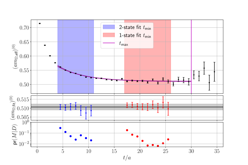
(a)

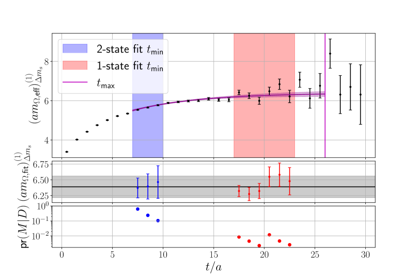
(b)

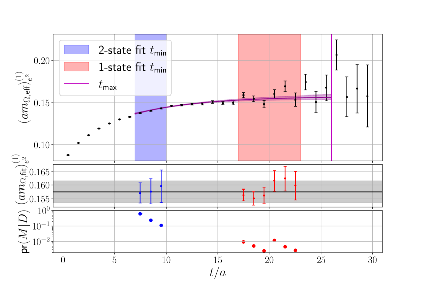
(c)

Figure 1: Example plots for the AIC model averages for the $\Omega$ baryon on the N200 ensemble. The top panels show the effective masses as defined in eq. 2 for the isospin-symmetric contribution (a), the $\Delta m_{s}$ correction (b), and the electromagnetic corrections (c). The blue and red bands show the ranges from which the values of $t_{\text{min}}$ were chosen, respectively. The purple vertical line shows the end of the fit intervals, which is common to all fits. The central panels show the results for the respective asymptotic mass for the individual fits where each point belongs to the fit starting at the the time $t/a$ shown on the abscissa. The bottom panels show the model weight for the respective fits as defined in eq. 5.

5 Results

As the goal of this project is to find a suitable quantity for setting the lattice scale on CLS ensembles with the inclusion of isospin breaking, we restrict our discussion on states which do not decay in QCD+QED. We summarize the currently achieved precision in table 2 for the asymptotic masses in isospin-symmetric QCD. In table 3 we focus on the $\Xi$ and $\Omega$ baryons which are promising candidates for scale setting due to their precision and, in the case of the $\Omega$, its weak dependence on the light-quark mass which results in a small isospin-breaking correction when compared to other baryons.

Table 2: Relative errors $\frac{\Delta(am_{i})^{(0)}}{(am_{i})^{(0)}}$ of the asymptotic masses of all stable octet- and decuplet-baryons in the isospin-symmetric theory obtained from AIC model averaged single- and two-state-fits. All quoted values ignore systematic contributions to the error, but include the variation from the different fits going into the average as per eq. 7.

Ensemble	$N$	$\Lambda$	$\Sigma$	$\Xi$	$\Omega$
D450	0.83%	0.67%	0.32%	0.28%	0.31%
N200	0.97%	0.37%	0.37%	0.24%	0.33%
N203	0.36%	0.28%	0.30%	0.24%	0.40%
N451	0.25%	0.17%	0.15%	0.34%	0.20%
N452	0.69%	0.38%	0.59%	0.24%	0.95%

Table 3: Relative errors $\frac{\Delta(am_{i})^{(1)}}{(am_{i})^{(1)}}$ of the isospin-breaking corrections to the the masses of the $\Xi$ and $\Omega$ baryons from AIC model averaged single- and two-state-fits. All quoted values ignore systematic contributions to the error, as well as contributions coming from corrections to the sea-quark sector, but include the variation from the different fits going into the average as per eq. 7.

Ensemble	$\Xi^{0}$			$\Xi^{-}$			$\Omega^{-}$
	$e^{2}$	$\Delta m_{u}$	$\Delta m_{s}$	$e^{2}$	$\Delta m_{d}$	$\Delta m_{s}$	$e^{2}$	$\Delta m_{s}$
D450	1.6%	2.2%	0.7%	0.9%	2.2%	0.7%	1.4%	1.7%
N200	1.5%	1.8%	0.9%	1.0%	1.7%	0.9%	2.5%	2.6%
N203	1.0%	1.2%	0.6%	0.8%	1.2%	0.6%	1.8%	1.8%
N451	1.8%	1.4%	1.5%	1.2%	1.4%	1.6%	0.9%	1.0%
N452	0.9%	1.0%	0.7%	0.6%	1.0%	0.7%	1.5%	2.4%

The precision quoted in these tables do not include systematic contributions to the uncertainty. However, from the typical size of the statistical errors we find that we can push all of the considered states below $1\text{\,}\%$ precision and, in the case of the $\Xi$, even below $0.5\text{\,}\%$ for the isospin-symmetric masses on all ensembles. The uncertainties in the isospin-breaking corrections are ususally $\mathcal{O}($1\text{\,}\%$)$, which we expect to be negligible when considering the full computation of the baryon masses in QCD+QED as these corrections are multiplied by expansion coefficients of $\mathcal{O}(10^{-3}-10^{-2})$, suppressing these uncertainties. Since we do not include any corrections in the sea-quark sector, these uncertainties are likely underestimated, but from the above argument, we would still expect the overall uncertainties to be subdominant to the isospin-symmetric contribution’s uncertainty.

6 Conclusion and Outlook

We have presented the status of our investigation of baryon octet- and decuplet-masses as candidates for scale setting on CLS $N_{f}=2+1$ ensembles with the inclusion of isospin-breaking effects. Given the high statistical precision we observe in the isospin-symmetric mass determinations and the relatively small size of isospin-breaking corrections, we are confident that we can achieve sub-percent precision for the lattice scale. Thus far, we only have data at two different lattice spacings of $\sim\!\!$0.064\text{\,}\mathrm{f}\mathrm{m}$$ and $\sim\!\!$0.076\text{\,}\mathrm{f}\mathrm{m}$$, but we intend to add further ensembles, allowing for a preliminary continuum extrapolation and better investigation of the precision we can achieve for the lattice scales using these baryon masses.

References

- [1] M. Cè et al., Window observable for the hadronic vacuum polarization contribution to the muon g-2 from lattice QCD, Phys. Rev. D 106 (2022) 114502 [2206.06582].
- [2] M. Della Morte, A. Francis, V. Gülpers, G. Herdoíza, G. von Hippel, H. Horch et al., The hadronic vacuum polarization contribution to the muon from lattice QCD, JHEP 10 (2017) 020 [1705.01775].
- [3] M. Bruno et al., Simulation of QCD with N 2 1 flavors of non-perturbatively improved Wilson fermions, JHEP 02 (2015) 043 [1411.3982].
- [4] M. Bruno, T. Korzec and S. Schaefer, Setting the scale for the CLS flavor ensembles, Phys. Rev. D 95 (2017) 074504 [1608.08900].
- [5] B. Strassberger et al., Scale setting for CLS 2+1 simulations, PoS LATTICE2021 (2022) 135 [2112.06696].
- [6] N. Carrasco, V. Lubicz, G. Martinelli, C.T. Sachrajda, N. Tantalo, C. Tarantino et al., QED Corrections to Hadronic Processes in Lattice QCD, Phys. Rev. D 91 (2015) 074506 [1502.00257].
- [7] G.M. de Divitiis et al., Isospin breaking effects due to the up-down mass difference in Lattice QCD, JHEP 04 (2012) 124 [1110.6294].
- [8] RM123 collaboration, Leading isospin breaking effects on the lattice, Phys. Rev. D 87 (2013) 114505 [1303.4896].
- [9] M. Luscher, S. Sint, R. Sommer and P. Weisz, Chiral symmetry and O(a) improvement in lattice QCD, Nucl. Phys. B 478 (1996) 365 [hep-lat/9605038].
- [10] J. Bulava and S. Schaefer, Improvement of = 3 lattice QCD with Wilson fermions and tree-level improved gauge action, Nucl. Phys. B 874 (2013) 188 [1304.7093].
- [11] APE collaboration, Glueball Masses and String Tension in Lattice QCD, Phys. Lett. B 192 (1987) 163.
- [12] S. Gusken, A Study of smearing techniques for hadron correlation functions, Nucl. Phys. B Proc. Suppl. 17 (1990) 361.
- [13] UKQCD collaboration, Gauge invariant smearing and matrix correlators using Wilson fermions at Beta = 6.2, Phys. Rev. D 47 (1993) 5128 [hep-lat/9303009].
- [14] Lattice Hadron Physics (LHPC) collaboration, Clebsch-Gordan construction of lattice interpolating fields for excited baryons, Phys. Rev. D 72 (2005) 074501 [hep-lat/0508018].
- [15] T. Blum, T. Izubuchi and E. Shintani, Error reduction technique using covariant approximation and application to nucleon form factor, PoS LATTICE2012 (2012) 262 [1212.5542].
- [16] T. Blum, T. Izubuchi and E. Shintani, New class of variance-reduction techniques using lattice symmetries, Phys. Rev. D 88 (2013) 094503 [1208.4349].
- [17] E. Shintani, R. Arthur, T. Blum, T. Izubuchi, C. Jung and C. Lehner, Covariant approximation averaging, Phys. Rev. D 91 (2015) 114511 [1402.0244].
- [18] M. Hayakawa and S. Uno, QED in finite volume and finite size scaling effect on electromagnetic properties of hadrons, Prog. Theor. Phys. 120 (2008) 413 [0804.2044].
- [19] A. Risch and H. Wittig, Towards leading isospin breaking effects in mesonic masses with open boundaries, PoS LATTICE2018 (2018) 059 [1811.00895].
- [20] A. Risch, Isospin breaking effects in hadronic matrix elements on the lattice, Ph.D. thesis, Mainz U., 2021. 10.25358/openscience-6314.
- [21] A. Risch and H. Wittig, Leading isospin breaking effects in the HVP contribution to and to the running of , PoS LATTICE2021 (2022) 106 [2112.00878].
- [22] A.M. Segner, A.D. Hanlon, A. Risch and H. Wittig, Setting the Scale Using Baryon Masses with Isospin-Breaking Corrections, PoS LATTICE2022 (2023) 084 [2212.07176].
- [23] G.P. Lepage, The Analysis of Algorithms for Lattice Field Theory, in Theoretical Advanced Study Institute in Elementary Particle Physics, 6, 1989.
- [24] M.L. Wagman and M.J. Savage, Statistics of baryon correlation functions in lattice QCD, Phys. Rev. D 96 (2017) 114508 [1611.07643].
- [25] L. Del Debbio, L. Giusti, M. Luscher, R. Petronzio and N. Tantalo, QCD with light Wilson quarks on fine lattices (I): First experiences and physics results, JHEP 02 (2007) 056 [hep-lat/0610059].
- [26] H. Akaike, Information Theory and an Extension of the Maximum Likelihood Principle, in Springer Series in Statistics, (New York), Springer Science+Business Media (1998), DOI.
- [27] W.I. Jay and E.T. Neil, Bayesian model averaging for analysis of lattice field theory results, Phys. Rev. D 103 (2021) 114502 [2008.01069].
- [28] E.T. Neil and J.W. Sitison, Improved information criteria for Bayesian model averaging in lattice field theory, 2208.14983.