Auto-Prox: Training-Free Vision Transformer Architecture Search via Automatic Proxy Discovery

Abstract

The substantial success of Vision Transformer (ViT) in computer vision tasks is largely attributed to the architecture design. This underscores the necessity of efficient architecture search for designing better ViTs automatically. As training-based architecture search methods are computationally intensive, there’s a growing interest in training-free methods that use zero-cost proxies to score ViTs. However, existing training-free approaches require expert knowledge to manually design specific zero-cost proxies. Moreover, these zero-cost proxies exhibit limitations to generalize across diverse domains. In this paper, we introduce Auto-Prox, an automatic proxy discovery framework, to address the problem. First, we build the ViT-Bench-101, which involves different ViT candidates and their actual performance on multiple datasets. Utilizing ViT-Bench-101, we can evaluate zero-cost proxies based on their score-accuracy correlation. Then, we represent zero-cost proxies with computation graphs and organize the zero-cost proxy search space with ViT statistics and primitive operations. To discover generic zero-cost proxies, we propose a joint correlation metric to evolve and mutate different zero-cost proxy candidates. We introduce an elitism-preserve strategy for search efficiency to achieve a better trade-off between exploitation and exploration. Based on the discovered zero-cost proxy, we conduct a ViT architecture search in a training-free manner. Extensive experiments demonstrate that our method generalizes well to different datasets and achieves state-of-the-art results both in ranking correlation and final accuracy. Codes can be found at https://github.com/lilujunai/Auto-Prox-AAAI24.

1 Introduction

Recently, Vision Transformer (ViT) (Dosovitskiy et al. 2020a) has achieved remarkable performance in image classification (Liang et al. 2022; Jiang et al. 2021; Chen, Fan, and Panda 2021), object detection (Wu et al. 2022), semantic segmentation (Dong et al. 2021), and other computer vision tasks (Li et al. 2021b; Liu et al. 2021b). Despite these advancements, the manual trial-and-error method of designing ViT architectures becomes impractical given the expanding neural architecture design spaces and intricate application scenarios (Liu et al. 2023; Li et al. 2023b; Li and Jin 2022; Li et al. 2023a, 2022d, 2022c; Li 2022; Shao et al. 2023). Neural Architecture Search (NAS) aims to address this issue by automating the design of neural network architectures. Traditional training-based architecture search methods (Xie et al. 2019; Wei et al. 2023; Hu et al. 2021; Dong et al. 2022; Chen et al. 2022; Dong, Li, and Wei 2023; Dong et al. 2023; Lu et al. 2024; Zimian Wei et al. 2024) involve training and evaluating numerous candidate ViTs, which can be computationally expensive and time-consuming. Therefore, there is a need for a more efficient architecture search of ViT.

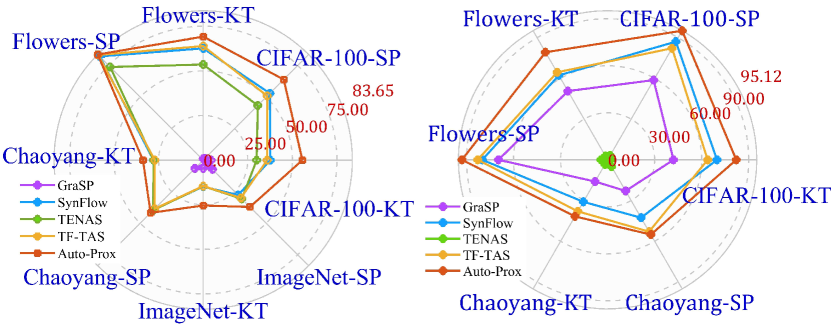
Figure 1: Kendall (KT) & Spearman (SP) ranking correlations of zero-cost proxies on AutoFormer (Left) and PiT (Right) search space for four datasets including CIFAR-100, Flowers, Chaoyang, and ImageNet. Results demonstrate that our proposed Auto-Prox significantly outperforms Synflow (Tanaka et al. 2020) and TF-TAS (Zhou et al. 2022).

Recent training-free NAS methods, such as NWOT (Mellor et al. 2021) and TF-TAS (Zhou et al. 2022), have received great research interest due to their meager costs. These methods utilize hand-crafted zero-cost proxies (Tanaka et al. 2020; Chen, Gong, and Wang 2020), which are conditional on the model’s parameters or gradients, to predict the actual accuracy ranking without the expensive training process. However, there are still some drawbacks limiting their broader application: (1) Dependency on expert knowledge and extensive tuning. Lots of traditional zero-cost proxies are transferred from different areas with extensive expert intuition and time-consuming tuning processes. In addition, these hand-crafted zero-cost proxies can be influenced by human biases and limited by the designer’s experience. (2) Generality and flexibility. Hand-crafted zero-cost proxies may perform well on the specific problem but can not generalize well to new or unseen datasets or tasks (see Figures 1). These zero-cost proxies usually have fixed formulas, and some do not associate with input or labels of the target dataset. i.e., scores of the same architecture on different datasets are the same, which does not match the facts. Thus, two problems are naturally raised: (1) How to efficiently discover the proxies without expert knowledge? (2) How to reduce the gap between fixed zero-cost proxy and variable tasks?

For the first problem, we propose Auto-Prox, a from-scratch automatic proxy search framework, as an alternative to traditional manual designs. Unlike hand-crafted zero-cost proxies, Auto-Prox mitigates human bias and automates the exploration of more expressive and efficient zero-cost proxies. First, we establish the ViT-Bench-101 dataset, which comprises diverse ViT architectures and their corresponding performance on multiple datasets. ViT-Bench-101 provides a benchmark for evaluating the score-accuracy correlations of different zero-cost proxies. We then define the zero-cost proxy search space, which includes ViT’s weights and gradient statistics as candidate inputs, potential unary and binary mathematical operations, and computation graphs as representations of zero-cost proxies. In our exploration of the proxy search space, we introduce an elitism preservation strategy to enhance search efficiency. This strategy involves judgment in the evolutionary search to preserve high-performing zero-cost proxies.

For the second problem, we propose a joint correlation metric, designed as the objective for the evolutionary proxy search. Instead of solely optimizing the automatic proxy based on high score-accuracy correlation within a single dataset, this metric captures the weighted average of correlations spanning multiple datasets. Based on the joint correlation metric, Auto-Prox improves generalization, allowing for discovering zero-cost proxies that perform well on new or unseen datasets or tasks.

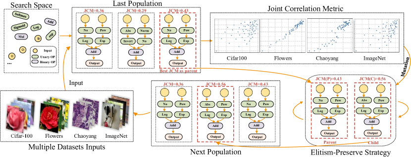
Figure 2: Illustration of the Auto-Prox search process. First, we devise a comprehensive search space, incorporating primitive operations, ViT statistics, and computation graphs to represent zero-cost proxies. We then randomly sample candidate zero-cost proxies to initialize the population and evaluate their ranking consistency using the Joint Correlation Metric across four datasets. Based on the JCM score, we pick up promising ones as parents and perform mutation to generate a new population. Subsequently, we perform the elitism-preserve strategy to prevent the deterioration of the population.

We conduct extensive experiments on CIFAR-100, Flowers, Chaoyang (Zhu et al. 2021), and ImageNet-1K to validate the superiority of our proposed method. For small datasets, except for ImageNet-1K, we focus on distillation accuracy instead of vanilla accuracy for ViTs, in contrast to traditional NAS experiments. The experiments demonstrate that our Auto-Prox can achieve better distillation accuracy than other zero-cost proxies when searched in the same search spaces. Moreover, Auto-Prox obtains state-of-the-art ranking correlation across multiple datasets, significantly surpassing existing training-free NAS approaches (see Figure 1) without prior knowledge.

Main Contributions:

• We focus on a training-free architecture search for ViTs across multiple datasets. We build ViT-Bench-101 and discover the failures in the generalization of existing training-free methods.

• We propose a from-scratch proxy search framework, Auto-Prox, designed to eliminate the need for manual intervention and enhance generalizability. We propose a joint correlation metric to evolve different zero-cost proxy candidates and an elitism-preserve strategy to improve search efficiency.

• We experimentally validate that Auto-Prox achieves state-of-the-art performance across multiple datasets and search spaces, advancing the broader application of ViTs in vision tasks.

2 Related Work

Vision Transformer (ViT) (Dosovitskiy et al. 2020a) has shown remarkable performance in various visual recognition tasks due to its ability to capture long-range dependencies. Recently, researchers have developed several automated techniques to discover more effective ViT architectures. For instance, AutoFormer (Chen et al. 2021a) utilizes a one-shot NAS framework for ViT-based architecture search, while BossNAS (Li et al. 2021a) incorporates a hybrid CNN-transformer search space along with a self-supervised training scheme. S3 (Chen et al. 2021c) proposes using neural architecture search to automate the design of superior ViT architectures, considering not just the architecture search but also the search space itself. ViTAS (Su et al. 2021b) has developed a cyclic weight-sharing mechanism for token embeddings of ViTs to stabilize the training of Superformer and prevent catastrophic failures. Despite significant progress in ViT architecture search, the aforementioned one-shot-based methods are still computationally demanding. TF-TAS (Zhou et al. 2022) stands as the first method to conduct a training-free architecture search for ViTs, assessing ViT by merging two theoretical perspectives: synaptic diversity from multi-head self-attention layers (MSA) and synaptic saliency from multi-layer perceptrons (MLP). However, current training-free ViT architecture search methods struggle to generalize across various domains. In this paper, we introduce an automated approach to pinpoint excellent proxies for ViTs across diverse datasets. Comparing with EZNAS: Auto-Prox differs notably from EZNAS (Akhauri et al. 2022) from the following aspects: (1) EZNAS is only designed for CNNs, but our approach is customized for ViTs. (2) EZNAS simply follows the search strategy from AutoML-Zero. In contrast, we propose an elitism-preserve strategy that significantly improves search efficiency and results (see Figure 5). (3) Our proposed Joint Correlation Metric enhances ranking consistency across multiple datasets, encompassing both small and large-scale datasets, such as ImageNet-1K. In contrast, EZNAS’s testing is limited to small datasets.

3 Methodology

In this section, we first introduce the search space of our automatic zero-cost proxy. We then delve into the details of the joint correlation metric and the elitism-preserve strategy during the evolutionary process. Subsequently, we give an analysis of the searched zero-cost proxy. Finally, we illustrate the training-free ViT search process.

Search Space of Automatic Zero-cost Proxy

To guarantee the effectiveness and flexibility of the zero-cost proxy search space, we begin with revisiting the formulations of existing zero-cost proxies. Using this foundational understanding, we design a search space that encompasses eight input candidates, and $56$ primitive operations. This comprehensive search space allows us to explore a wide range of zero-cost proxies, uncovering potential ones that previous hand-crafted approaches may have overlooked.

Review of Existing Zero-cost Proxies

To investigate the design of zero-cost proxies, we summarize the existing ones in Table 1. Among these zero-cost proxies, Fisher (Theis et al. 2018), SNIP (Lee, Ajanthan, and Torr 2018), Plain (Mozer and Smolensky 1988), and SynFlow (Tanaka et al. 2020) are conducted on ReLU-Conv2D-BatchNorm2D blocks in CNNs. In contrast, TF-TAS (Zhou et al. 2022) is based on transformer layers in ViTs. The inputs of these zero-cost proxies derive from the following types of network statistics: Activation (A), Gradient (G), and Weight (W). Specifically, Fisher computes the sum over all gradients of the activations $\frac{\partial\mathcal{L}}{\partial z}$ in the network, which can be used for channel pruning. SNIP, employing weight $\theta$ and gradient $\frac{\partial\mathcal{L}}{\partial\theta}$ as inputs, computes a saliency metric at initialization using a single mini-batch of data. This metric approximates the change in loss when a specific parameter is removed. SynFlow, also using weight $\theta$ and gradient $\frac{\partial\mathcal{R}}{\partial\theta}$ as inputs, introduces a modified version of synaptic saliency scores to prevent layer collapse during parameter pruning. TF-TAS considers the weights $\theta_{l},\theta_{k}$ and their gradients $\frac{\partial\mathcal{L}}{\partial\theta_{l}},\frac{\partial\mathcal{L}}{\partial\theta_{k}}$ from multi-head self-attention (MSA) and multi-layer perceptron (MLP) as inputs, respectively. $\left\|\right\|_{n}$ is the Nuclear-norm.

Input	Proxy	Formula
A&G	Fisher (Theis et al. 2018)	$\sum_{z\in A}{\left(\frac{\partial\mathcal{L}}{\partial z}z\right)^{2}}$
W&G	SNIP (Lee, Ajanthan, and Torr 2018)	$\left|(\frac{\partial\mathcal{L}}{\partial\theta})\odot\theta\right|$
W&G	Plain (Mozer and Smolensky 1988)	$(\frac{\partial\mathcal{L}}{\partial\theta})\odot\theta$
W&G	SynFlow (Tanaka et al. 2020)	$(\frac{\partial\mathcal{R}}{\partial\theta})\odot\theta,\mathcal{R}=\mathds{1}^{T}\left(\prod_{\theta_{i}\in W}\left|\theta_{i}\right|\right)\mathds{1}$
W&G	TF-TAS (Zhou et al. 2022)	$\sum_{\theta_{l}}{\left\|(\frac{\partial\mathcal{L}}{\partial\theta_{l}})\right\|_{n}\odot\left\|\theta_{l}\right\|_{n}}+\sum_{\theta_{k}}{(\frac{\partial\mathcal{L}}{\partial\theta_{k}})\odot\theta_{k}}$

Table 1: Overview of existing zero-cost proxies. A, W, and G refer to Activation, Weight, and Gradient.

ViT Statistics as Input

The input subsection in Table 1 explores the input choices for constructing zero-cost proxies, in which activations (A), gradients(G), and weights(W) are identified as the most informative and effective options. Activation provides insight into the data distribution and internal network representations, while gradients highlight the sensitivity of weights to the loss functions, and weights reflect the significance of network parameters. Building on this observation, we register the activation, weights, and corresponding gradients from each transformer layer as potential inputs of our zero-cost proxy. For modules in the multi-head self-attention (MSA), we collect their weights and gradients at initialization using a mini-batch of data. Regarding multi-layer perception (MLP), we consider weights, gradients, activation, and activation gradients as possible inputs. To differentiate between these inputs, we employ symbols like F1 and F1g. As depicted in Figure 3, for a transformer layer, there are a total of eight potential inputs in the zero-cost proxy search space.

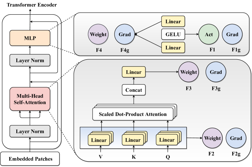
Figure 3: ViT statistics of the zero-cost proxy search space, including activation (Act), gradient (Grad), and weights (Weight) from MSA and MLP modules.

Primitive Operations

To efficiently aggregate information from different types of inputs, we search among different primitive operations to produce the final scalar output. In the context of the zero-cost proxy, primitive operations are used to process ViT statistics, resulting in the zero-cost proxy score for performance evaluation. We consider two types of primitive operations, including unary operations (operations with only one operand) and binary operations (operations with two operands). Inspired by AutoML-based methods (Li et al. 2022a; Real et al. 2020; Dong et al. 2023), we provide a total of $24$ unary operations and four binary operations to form the zero-cost proxy search space. Since the intermediate variables can be scalar or matrix, the total number of operations is $56$. All the primitive operations in the zero-cost proxy search space are described in Appendix G.

Zero-cost Proxy as Computation Graph.

The automatic zero-cost proxy is represented as a computation graph, in which the input nodes are ViT statistics, and the intermediate nodes are primitive operations. The graph’s output yields the proxy score used for ViT ranking. There are four main types of computation graphs, namely Linear, Tree, Graph (DAG), and unstructured memory-based structures (such as Automl-zero (Real et al. 2020)). The expressiveness of the computation graph increases from Linear to unstructured memory-based structures, but the valid structure in the search space decreases. To balance the trade-off between expressiveness and validity, we employ an expression tree to represent the automatic zero-cost proxy. Based on previous works such as SNIP (Lee, Ajanthan, and Torr 2018), and TF-TAS (Zhou et al. 2022), most proxies typically require two types of inputs. Therefore, we build an expression tree with two inputs (see Figure 2). The expression tree is applied to every transformer layer of ViT, with the final proxy score derived by averaging the outputs from all transformer layers.

Algorithm 1 Evolutionary Search for Auto-Prox

Input: Search space $\mathcal{S}$, population $\mathcal{P}$, max iteration $\mathcal{T}$, sample ratio $r$, sampled pool $\mathcal{R}$, topk $k$, margin $m$.

Output: Auto-prox with best JCM.

1:  $\mathcal{P}0$ := Initialize population$(P_{i})$;

2:  Sample pool $\mathcal{R}$ := $\emptyset$;

3:  for $i=1,2,\ldots,\mathcal{T}$ do

4:     Clear sample pool $\mathcal{R}$ := $\emptyset$;

5:     Randomly select $\mathcal{R}\in\mathcal{P}$;

6:     Candidates ${G_{i}}{k}$ := GetTopk($\mathcal{R}$, $k$);

7:     Parent $G_{i}^{p}$ := RandomSelect$({G_{i}}_{k})$;

8:     Mutate $G_{i}^{m}$ := MUTATE($G_{i}^{p}$);

9:     // Elitism-Preserve Strategy.

10:     if $\mathrm{JCM}(G_{i}^{m})-\mathrm{JCM}(G_{i}^{p})\geq m$ then

11:        Append $G_{i}^{m}$ to $P$;

12:     else

13:        Go to line 8;

14:     end if

15:     Remove the zero-cost proxy with the lowest JCM.

16:  end for

Evolving Automatic Proxy on Multiple Datasets

Figure 2 presents the automatic proxy search. At initialization, we randomly sample a population of $N$ candidate zero-cost proxies from the search space, ensuring that they are valid primitively. Each of these proxies is then evaluated using the proposed Joint Correlation Metric, which serves as the fitness measure in our evolutionary search process. In each iteration of the evolutionary process, the top-k candidates with the highest JCM scores are selected. From this subset, a parent is randomly picked for mutation. When conducting mutation, a random point in the computation graph is chosen and mutated using new inputs or primitive operations. To guarantee the quality of mutated zero-cost proxies and stave off degradation, we’ve introduced the Elitism-Preserve Strategy. This strategy involves judgment and selectively retaining only valid and promising zero-cost proxies for the next generation. We repeat this process for $T$ iterations to identify the target zero-cost proxy. In the following, we introduce details of the Joint Correlation Metric and Elitism-Preserve Strategy.

Joint Correlation Metric (JCM)

Instead of measuring ranking correlation in just one dataset, we propose the Joint Correlation Metric (JCM), which measures the generalization of proxies $\mathcal{Q}$ among multiple datasets. We use $M$ datasets $\{\mathcal{D}_{i}\}_{i=0}^{M}$ and the weight $\{\alpha_{i}\}_{i=0}^{M}$ to measure the corresponding importance of datasets. JCM is formulated as the weighted sum of the ranking correlation (Kendall’s Tau $\tau$) as follows:

$$JCM(\mathcal{Q})=\frac{1}{M}\sum_{i}^{M}\alpha_{i}\times\tau(\mathcal{D}_{i},\mathcal{Q})$$ (1)

where $\tau$ is the ranking correlation between the zero-cost proxy score and actual accuracy on dataset $\mathcal{D}_{i}$.

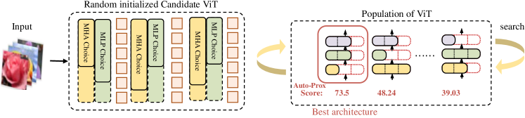
Figure 4: Illustration of the training-free ViT search process. Left: The search space of ViT, where multi-self attention and multi-layer perceptron are mutable. Right: Traverse the search space and select the best ViT with the highest Auto-Prox score.

Elitism-Preserve Strategy

To prevent population deterioration and premature convergence, the proposed Elitism-Preserve Strategy involves comparing the performance of the parent and newly generated offspring to measure the validity of the mutation. If the offspring is invalid or if its performance is lower than that of the parent, the mutation is considered as deterioration, and therefore new offspring are generated as a replacement. Algorithm 1 presents the detailed process.

Analysis of the Searched Zero-cost Proxy

Auto-Prox needs ViT statistics as its input. To eliminate the potential bias introduced by ViTs from a specific design space, we sampled ViT-accuracy configurations from two distinct design spaces of ViT-Bench-101 and performed zero-cost proxy searches on each. As a result, we discovered two separate zero-cost proxies, AutoProxA and AutoProxP, which are used independently to score ViTs sampled from their corresponding search spaces. It is important to note that Auto-Prox is an automated, from-scratch method, making it versatile across different ViT search spaces and datasets. Below, we present the formulas for the searched proxies within the AutoFormer (AutoProxA) and PiT search spaces (AutoProxP):

$${\rm AutoProxA}=|\frac{\partial\mathcal{L}}{\partial\theta_{l}}|+\frac{1}{n+\epsilon}\sum_{i=1}^{n}{sigmoid\left(\frac{\partial\mathcal{L}}{\partial\theta_{k}}\right)}$$ (2)

$${\rm AutoProxP}=\left\|sigmoid\left(\theta_{l}\right)\right\|_{F}-\log\left(\frac{\exp\left(\left\|\theta_{k}\right\|\right)}{\sum_{i}{\exp\left(\left\|\theta_{k}\right\|\right)}}\right)$$ (3)

where $\theta_{l}$ is the weight parameter matrix of QKV layers in the multi-head self-attention (MSA) module, $\frac{\partial\mathcal{L}}{\partial\theta_{l}}$ is the corresponding gradient matrix. $\theta_{k}$ is the weight parameter matrix of linear layers in the MLP module. $\frac{\partial\mathcal{L}}{\partial\theta_{k}}$ represents the corresponding gradient matrix. $n$ is the number of elements. $\epsilon$ is the constant set as $1e$-$9$. $\sum_{i}$ means the sum of elements in the i-th dimension. $\left\|\right\|_{F}$ means the Frobenius-norm.

By analyzing the formulas, we found that high-performing ViTs correlate positively with the following factors: (1) A larger norm of weight parameters or gradients in QKV layers of the MSA module, which approximately indicates the diversity of MSA (Dong, Cordonnier, and Loukas 2021). (2) More salient weight parameters in linear layers of the MLP module, implying a significant impact on performance. Moreover, we compare the searched proxies with existing TF-TAS  (Zhou et al. 2022), which is hand-crafted and is included in our zero-cost proxy search space. Table 3 and Table 2 have demonstrated the superiority of Auto-Prox, which significantly outperforms the TF-TAS method and meanwhile enjoys more search efficiency, further emphasizing the advantages of automatic searching.

Training-free ViT Search

Once we have obtained a good zero-cost proxy through the evolutionary search, we utilize it to perform a training-free ViT search. Figure 4 presents the training-free ViT search process. Specifically, we randomly explore a large number of candidate architectures from the ViT search space. Then, we evaluate each ViT architecture and select the best one based on the searched zero-cost proxy (Auto-Prox) score. Without the need for costly and time-consuming training, the ViT search process is highly efficient.

Search Space	Proxy	CIFAR-100			Flowers			Chaoyang
		Kendall	Spearman	Pearson	Kendall	Spearman	Pearson	Kendall	Spearman	Pearson
AutoFormer	GraSP	0.84±0.73	1.35 ±0.92	0.82 ±1.58	0.82±1.58	-7.33±0.10	-4.14±0.84	-4.42±0.38	-6.53±0.36	6.26±0.72
	SynFlow	37.66±0.63	52.89±1.11	52.01±0.74	62.59±0.01	82.13±0.01	62.26±7.71	27.87±0.75	39.30±1.51	41.08±1.14
	TENAS	-30.03±0.28	-43.27±0.46	-42.66±0.26	-53.55±0.05	-73.79±0.11	-54.17±8.31	-27.81±0.11	-39.69±0.24	-40.79±0.18
	NWOT	54.65±0.22	63.11±0.26	60.01±0.17	68.16±0.03	82.06±1.07	53.91±7.46	27.29±0.25	38.96±0.53	40.57±0.56
	TF-TAS	35.89±0.26	50.84±0.58	50.51±0.46	63.90±0.04	83.28±0.09	62.80±8.58	27.14±0.35	38.52±0.68	40.57±0.40
	Ours	55.67±0.74	63.87±1.04	60.56±0.93	69.19±2.03	83.65±0.93	79.52±7.15	33.76±0.46	41.76±0.66	42.63±0.45
PiT	GraSP	-42.02±0.58	-58.71±0.74	-31.53±0.09	-50.66±0.07	-69.64±0.09	-40.90 ±0.57	-16.00±0.61	-22.94±1.33	-19.07±0.56
	SynFlow	69.79±1.16	87.05±0.77	70.80±0.08	62.22±2.38	79.98±2.16	71.66±0.99	30.96±4.38	42.66±8.46	39.24±5.89
	TENAS	-2.13±0.30	-3.21±0.74	-1.68±0.17	-2.86±0.63	-4.23±1.46	-3.33±1.49	-3.34±0.03	-5.04±0.07	-3.55±0.13
	NWOT	-2.61±0.01	-4.13±0.01	-0.52±1.04	2.67±0.23	3.69±0.49	0.71±0.46	4.73±0.16	6.87±0.31	4.43±0.26
	TF-TAS	63.83±0.06	82.20±0.04	58.37±1.84	64.48±0.08	82.91±0.06	67.23±0.79	37.99±1.54	52.92±2.54	42.68±0.62
	Ours	82.07±0.33	95.12±0.09	73.25±1.30	79.25±0.94	92.94±0.33	79.53±0.14	41.67±4.45	55.09±7.50	49.17±3.94

Table 2: Ranking correlation results (%) on CIFAR-100, Flowers, and Chaoyang. Auto-Prox achieves the highest ranking correlation with distillation accuracy on all three datasets of the ViT-Bench-101, demonstrating superior generalization.

Search Space	Proxy	CIFAR-100			Flowers			Chaoyang
		Param(M)	Dis.Acc(%)	Search Cost	Param(M)	Dis.Acc(%)	Search Cost	Param(M)	Dis.Acc(%)	Search Cost
AutoFormer	Random	8.30	76.72	N/A	6.18	67.64	N/A	6.54	84.20	N/A
	GraSP	5.77	77.53	2.62 h	5.29	66.08	2.71 h	6.12	84.81	1.52 h
	SynFlow	9.52	77.83	1.91 h	8.13	68.61	1.85 h	5.82	83.87	1.77 h
	TENAS	5.40	75.54	4.83 h	5.25	66.69	4.82 h	5.16	84.53	4.80 h
	NWOT	8.36	76.79	3.24 h	8.87	69.18	3.24 h	5.53	84.71	3.07 h
	TF-TAS	5.25	75.72	1.94 h	5.80	67.57	1.87 h	5.60	84.57	1.92 h
	Ours	9.11	78.26	0.70 h	9.80	69.71	0.85 h	8.97	84.85	0.85 h
PiT	Random	5.33	75.84	N/A	4.88	65.30	N/A	5.24	82.94	N/A
	GraSP	4.53	76.03	1.24 h	3.72	66.58	1.85 h	4.63	83.87	0.86 h
	SynFlow	11.05	77.13	1.08 h	5.23	68.12	0.99 h	4.93	83.73	0.70 h
	TENAS	6.93	76.09	5.14 h	4.26	68.03	5.14 h	6.76	83.64	5.07 h
	NWOT	5.21	76.64	3.02 h	10.77	67.72	3.09 h	6.37	83.31	3.08 h
	TF-TAS	16.07	77.06	1.21 h	10.30	68.21	0.95 h	4.32	84.34	0.71 h
	Ours	6.22	77.26	0.51 h	6.20	68.85	0.39 h	4.49	84.53	0.31 h

Table 3: Comparing the distillation performance on three datasets of ViTs sampled from Autoformer and PiT search spaces, Auto-Prox achieves competitive results with the lowest search cost (measured on a single NVIDIA A40 GPU).

4 Experiments

ViT-Bench-101

ViT-Bench-101 provides ground-truth accuracy of ViTs on both tiny datasets and large-scale datasets. For the tiny datasets, we employ CIFAR-100 (Krizhevsky 2009), Flowers (Nilsback and Zisserman 2008), and Chaoyang (Zhu et al. 2021), while for the large-scale datasets, we focus on ImageNet-1K. Motivated by findings from (Li et al. 2022b), which show that ViTs achieve significant gains on tiny datasets when distilled from an efficient CNN teacher network, we include distillation accuracy for ViTs on these datasets using a given teacher. Specifically, for the smaller datasets excluding ImageNet-1K, ViT-Bench-101 offers both distillation accuracy and vanilla accuracy for ViTs sampled from AutoFormer and PiT search spaces. This supports the evaluation of zero-cost proxies based on the score-accuracy correlation in different scenarios, with or without distillation. Regarding the ImageNet-1K dataset, we follow the demonstration in (Chen et al. 2021a; Zhou et al. 2022), showing that the sub-nets with inherited weights from the pre-trained AutoFormer supernet can achieve performance comparable to the same network when retrained from scratch. Thus, we sample ViTs from the AutoFormer search space and collect their performance by inheriting weights from the publicly available supernet. ViT-Bench-101 contains 500 ground-truths for each dataset, facilitating fair comparisons between different zero-cost proxies and identifying high-performing ViTs. For more information on the training details for each dataset included in ViT-Bench-101, please refer to Appendix A.

Implementation Details

Evolutionary Zero-cost Proxy Search We partition the whole ViT-Bench-101 dataset into a validation set (60%) for proxy searching and a test set (40%) for proxy evaluation. There is no overlap between these two sets. In the evolutionary search process, we employ a population size of $\mathcal{P}=20$, and the total number of iterations $\mathcal{T}$ is set to $200$. To evaluate zero-cost proxy candidates, we randomly sample $100$ ViT ground-truth configurations from ViT-Bench-101 and measure the ranking consistency between its zero-cost proxy score and actual accuracy. We then calculate the Joint Correlation Metric based on the ranking consistencies on multiple datasets as the fitness function. When conducting mutation, the probability of mutation for a single node in a zero-cost proxy representation is set to $0.5$. The margin $m$ in the Elitism-Preserve Strategy is $0.1$. The zero-cost proxy search process is conducted on a single NVIDIA A40 GPU and occupies the memory of only one ViT.

Training-free ViT Search Based on the Auto-Prox score, the ViT search process is efficient since gradient back-propagation is not included. we randomly sample 400 ViTs from AutoFormer (Chen et al. 2021a) and PiT (Zhou et al. 2022) search spaces. The parameter intervals of ViTs from AutoFormer and PiT search spaces in our experiments are $4\sim 9$ M and $2\sim 25$ M, respectively. The final accuracy of the ViTs with the highest zero-cost proxy scores is reported as the results of the ViT search process. The hyperparameters for ViT retraining and building ViT-Bench-101 are adopted from (Li et al. 2022b).

Models	Param (M)	Acc (%)	GPU Days
Deit-Ti (Touvron et al. 2021)	5.7	72.2	-
TNT-Ti (Han et al. 2021)	6.1	73.9	-
ViT-Ti (Dosovitskiy et al. 2020b)	5.7	74.5	-
PVT-Tiny (Wang et al. 2021)	13.2	75.1	-
ViTAS-C (Su et al. 2021a)	5.6	74.7	32
AutoFormer-Ti (Chen et al. 2021b)	5.7	74.7	24
TF-TAS-Ti (Zhou et al. 2022)	5.9	75.3	0.5
Auto-Prox (Ours)	6.4	75.6	0.1

Table 4: ImageNet results on the AutoFormer search space.

Method	Kendall	Spearman	Pearson
Snip	14.61±1.55	30.62±6.03	49.45±10.68
SynFlow	14.81±2.33	27.69±7.25	44.19±10.35
NWOT	13.34±0.08	19.79±1.53	38.39±9.94
TF-TAS	14.52±1.74	29.93±6.38	48.70±11.04
Auto-Prox (ours)	25.44±0.90	37.10±1.86	51.84±10.07

Table 5: Ranking Correlation Results (%) for ImageNet-1K dataset in ViT-Bench-101.

Experimental Results on Tiny Datasets

Table 3 presents a comparison of distillation results obtained by using various zero-cost proxies on AutoFormer and PiT search spaces. In addition, we evaluate the ranking correlations of these zero-cost proxies under different experimental settings using metrics such as Kendall’s tau (Abdi 2007), Spearman’s rho (Stephanou and Varughese 2021), and Pearson’s correlation coefficient (Bowley 1928). As shown in both Table 2 and Figure 6, Auto-Prox outperforms other excellent zero-cost proxies. These findings demonstrate the importance of using effective zero-cost proxies and the superiority of Auto-Prox in achieving higher performance in ViT architecture search.

Experimental Results on ImageNet-1K

To validate the effectiveness and superiority of our proposed Auto-Prox further, we evaluate its performance on the challenging ImageNet-1K dataset, comparing its ranking correlation and top-1 classification accuracy with other hand-crafted and automatically searched ViT methods. The results, as presented in Table 4, demonstrate that the optimal ViT architecture searched by Auto-Prox outperforms both excellent hand-crafted and other automatically searched ViT methods, underscoring the superiority of our proposed approach. Importantly, our approach strikes a good balance between performance and search efficiency, requiring only 0.1 GPU days for ViT architecture search, making it a practical and efficient approach for ViT architecture search. Furthermore, the ranking correlation results in Table 5 show that our proposed Auto-Prox performs better than other zero-cost proxies on the challenging ImageNet task, further validating the effectiveness and generalization of our approach.

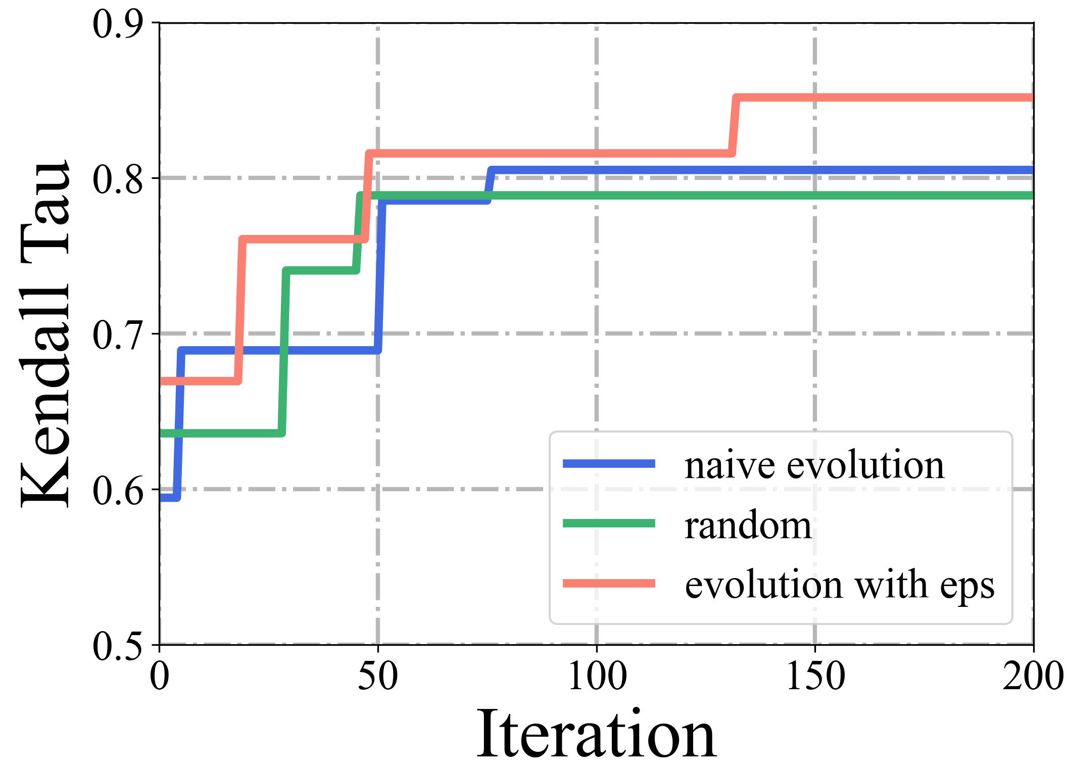
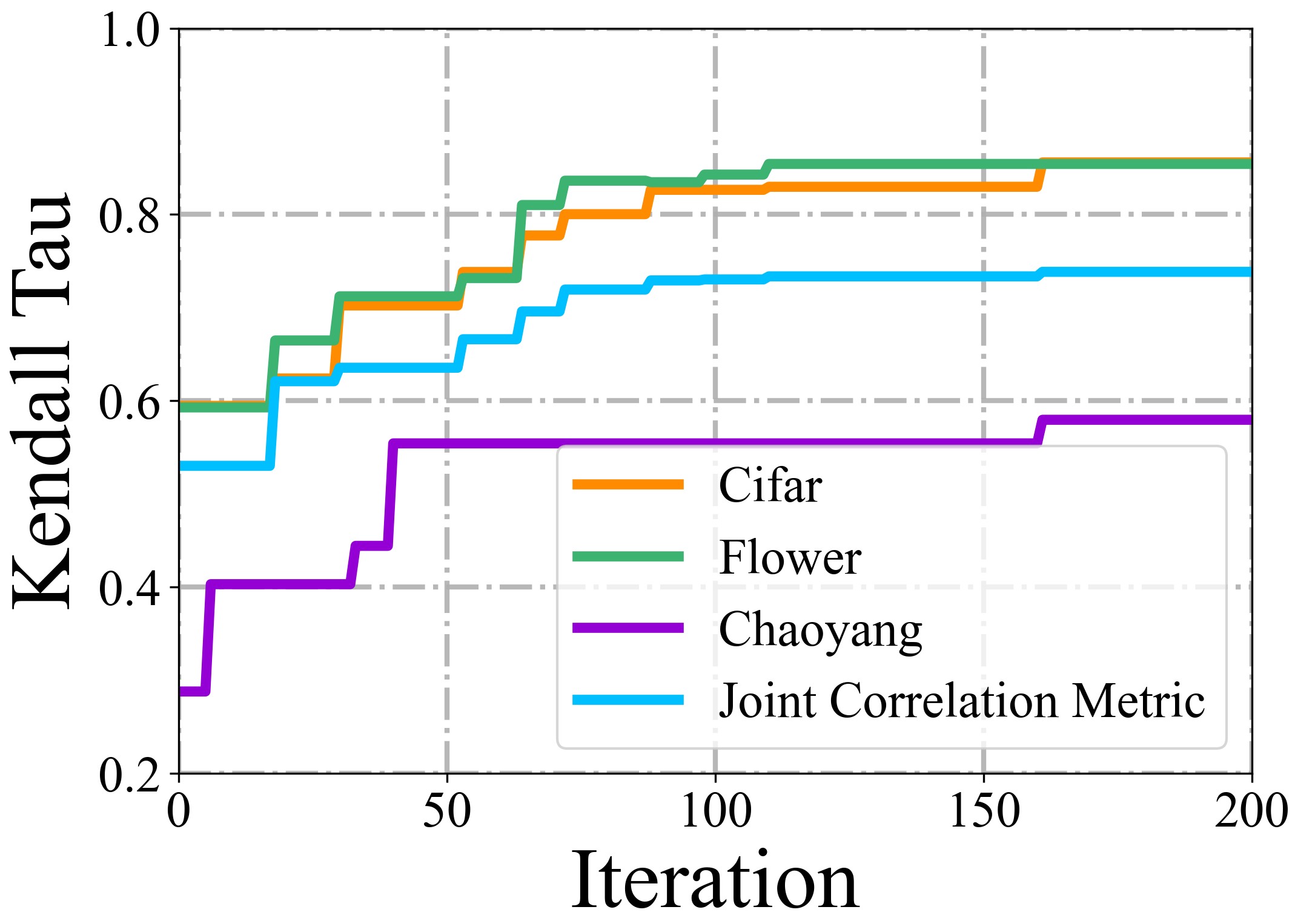
Figure 5: Left: Comparison of naive evolutionary search, random search, and evolutionary search with Elitism-Preserve Strategy, which is denoted as ’eps’. Right: Evolutionary process of ranking correlations on different datasets, and the proposed joint correlation metric.

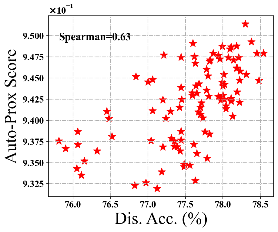
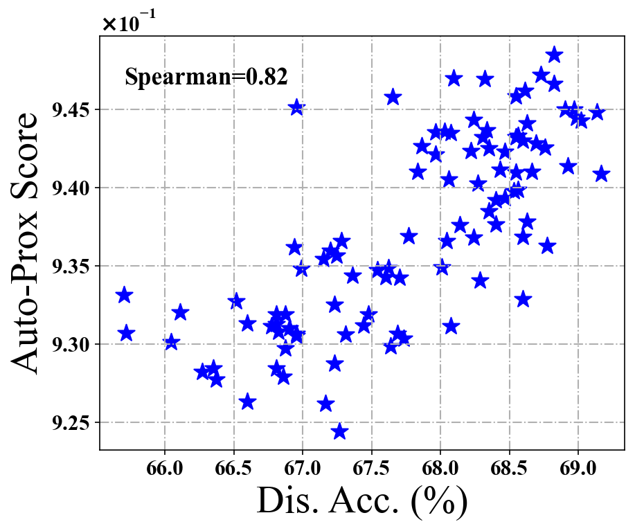
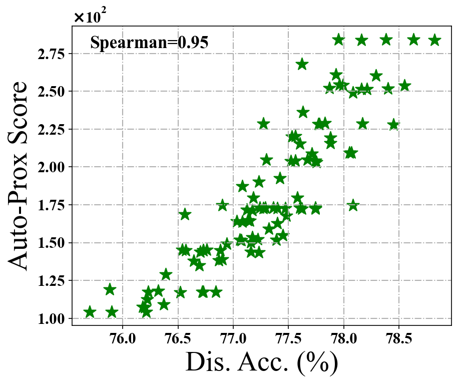
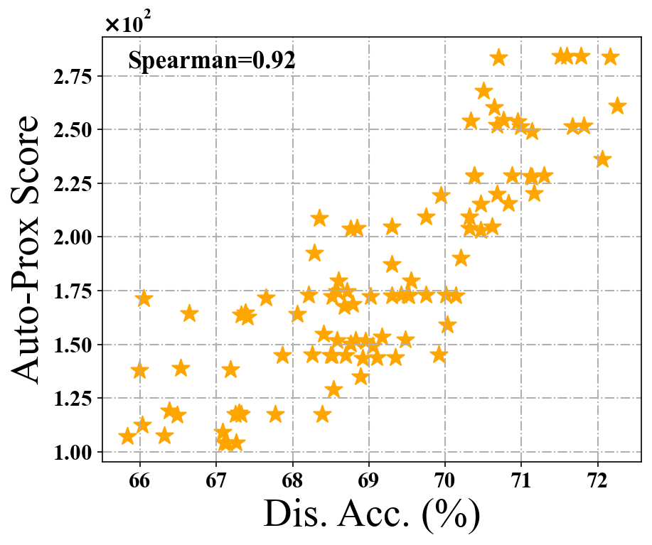
Figure 6: Correlation of distillation accuracy and Auto-Prox scores on AutoFormer search space (top left: CIFAR-100, top right: Flowers) and PiT search space (bottom left: CIFAR-100, bottom right: Flowers).

Method	CIFAR-100	Flowers	Chaoyang
SynFlow	86.88±1.55	86.57±2.38	64.51±4.96
NWOT	-0.45±8.08	1.98±6.55	-2.26±10.63
TF-TAS	84.79±4.57	86.51±3.74	69.09±7.05
Ours	91.01±2.63	90.70±1.96	76.95±6.54

Table 6: Spearman correlation results (%) with vanilla accuracy (without distillation). ViT-accuracy configurations are sampled from the PiT search space of ViT-Bench-101.

Ablation Study

As shown in Figure 5 (left), we observe that the proposed elitism-preserve strategy significantly enhances search efficiency, leading to better results. The findings underscore the importance of preserving the top-performing zero-cost proxies during the evolutionary process to achieve better search efficiency. Moreover, Figure 5 (right) reveals that optimizing the Joint Correlation Metric facilitates the discovery of high-performing zero-cost proxies across multiple datasets. We also conducted a zero-cost proxy search using vanilla accuracy provided by ViT-Bench-101. The results presented in Table 6 demonstrate the superior performance of Auto-Prox in the scenario without distillation.

5 Conclusion

In this paper, we present Auto-Prox, an automated proxy discovery framework designed for generality across multiple data domains. To facilitate the evaluation of zero-cost proxies, we propose the ViT-Bench-101 dataset as a standardized benchmark. We design a search space of automatic zero-cost proxies for ViTs and develop a joint correlation metric to optimize genetic proxy candidates. Additionally, we introduce an elitism preservation strategy to enhance search efficiency. With the searched proxy, we conduct a ViT architecture search in a training-free manner, achieving significant accuracy gains. Extensive experiments validate the efficiency and effectiveness of Auto-Prox across multiple datasets and search spaces. We hope this elegant and practical approach will inspire more investigation into the generalization of training-free ViT search methods.

6 Acknowledgements

This work is supported by the National Natural Science Foundation of China (No.62025208), the Open Project of Key Laboratory (2022-KJWPDL-06), and the Xiangjiang Laboratory Fund (No.22XJ01012).

Appendix

In this appendix, we provide additional details about Auto-Prox. Namely, we first introduce ViT-Bench-101, the dataset used for evaluating different zero-cost proxies. Then, we elaborate on primitive operations, ranking correlation metrics, computation graph details, and the validity check. Additionally, we present more ablation studies, including the sensitivity analysis of seeds, more evolutionary iterations, and application to larger ViTs. Lastly, we present ViTs that were searched in two search spaces with Auto-Prox.

Appendix A Details of ViT-Bench-101

ViT-Bench-101 evaluates each ViT architecture on four datasets. It serves as a benchmark for zero-cost proxies by analyzing the ranking correlation between their proxy scores and accuracies, and also enables different NAS algorithms to identify high-performing ViTs.

Datasets

We choose the most popular image classification datasets, including CIFAR-100 (Krizhevsky and Hinton 2009), Oxford Flowers (Krizhevsky et al. 2009), Chaoyang (Zhu et al. 2021), and ImageNet-1K (Deng et al. 2009). CIFAR-100 contains 50,000 training samples and 10,000 test samples across 100 classes. Oxford Flowers comprises 2,040 training samples and 6,149 test samples for 102 classes. Chaoyang, which falls within the medical image domain, includes 4,021 training samples and 2,139 test samples, distributed among four classes. The ImageNet-1K dataset spans 1,000 object classes and consists of 1,281,167 training images, 50,000 validation images, and 100,000 test images.

ViT Search Space

We conduct experiments on AutoFormer (Chen et al. 2021a), and PiT (Zhou et al. 2022) search spaces. Their detailed, searchable components are presented in Table 7.

• AutoFormer: The variable factors of basic transformer blocks include the embedding dimension (ranging from $192$ to $240$, with a step of $24$), Q-K-V dimension (ranging from $192$ to $256$, with a step of $64$), number of heads (ranging from $3.5$ to $4$, with a step of $0.5$), and MLP ratio (ranging from $3$ to $4$, with a step of $1$). The network depth varies between 12 and 14 layers.

• PiT: The searchable PIT transformer blocks include the base dim (ranging from $16$ to $40$, with a step of $8$), and the MLP ratio (ranging from $2$ to $8$, with a step of $2$). The number of heads can be selected from the set {2,4,8}. The depth choices for the three stages of PIT are {1,2,3}, {4,6,8}, and {2,4, 6}.

Table 7: Searchable components of the AutoFormer and PiT search space. Tuples of three values in parentheses represent the lowest value, highest, and steps. Meanwhile, values in curly brackets represent a set of all possible options.

AutoFormer		PiT
Embed Dim	(192, 240, 24)	Base Dim	(16, 40, 8)
$Q$-$K$-$V$ Dim	(192, 256, 64)	Patch Size	16
MLP Ratio	(3.5, 4, 0.5)	MLP Ratio	(2, 8, 2)
Head Num	(3, 4, 1)	Head Num	{2,4,8}
Depth Num	(12, 14, 1)	Depth Num	{{1,2,3},{4,6,8},{2,4,6}}
Params Range	4 – 9M	Params Range	2 – 25M

Training settings

Vanilla Training settings

Vanilla training refers to a standard training procedure in which a ViT model learns directly from labeled data, with no external guidance or prior knowledge. The loss function in this approach typically measures the discrepancy between predicted and true labels, with the optimization process seeking to minimize this loss. For all ViT models, we follow the training settings described in (Liu et al. 2021a). More specifically, we use the AdamW optimizer (Loshchilov and Hutter 2017) with an initial learning rate of 5e-4 and a weight decay of 0.05. We employ a cosine policy (Loshchilov and Hutter 2016) for the learning rate schedule, eventually reducing the learning rate to 5e-6. Each ViT is trained for a total of 300 epochs, with a linear warm-up period of 20 epochs, using a batch size of 128. We train on images with an interpolated resolution of $224\times 224$.

Distillation Training settings

Distillation training is a specialized training approach in which a student model (in this case, the ViT) is trained under the guidance of a pre-trained teacher model. During distillation training, the loss function incorporates both the standard supervised loss, based on the labeled data, and a distillation loss, based on the teacher model’s predictions. We adopt the distillation technique proposed in (Li et al. 2022b). This method utilizes a lightweight CNN to provide local information to significantly improve the performance of the ViTs, particularly on small datasets. The training hyper-parameters for ViTs are the same as those used in vanilla training. When training the CNN teacher (ResNet56), we use the SGD optimizer with an initial learning rate of 0.1 and a weight decay of 5e-4. The CNN teacher takes low-resolution images ($32\times 32$) as inputs, which facilitates efficient training. The hyper-parameters and training strategies for both ViTs and ResNet56 are summarized in Table 8.

Table 8: The training hyper-parameters on datasets including CIFAR-100, Oxford Flowers, and Chaoyang.

ViT		ResNet56
optimizer	AdamW	optimizer	SGD
input size	$224\times 224$	input size	$32\times 32$
initial lr	5e-4	base lr	0.1
ending lr	5e-6	momentum	0.9
warm-up	20	nesterov	True
weight decay	0.05	weight decay	5e-4
batch size	128	batch size	128
epoch	300	epoch	300
LR schedule	cosine	LR schedule	cosine

Table 9: ViT-Bench-101 provides the following metrics. ‘Dis Acc’ means accuracy obtained with distillation.

Search Space	Num	Dataset	Metric
AutoFormer	500	CIFAR-100	Dis Acc, Vanilla Acc
		Flowers	Dis Acc, Vanilla Acc
		Chaoyang	Dis Acc, Vanilla Acc
		ImageNet-1K	Subnet Acc
PiT	500	CIFAR-100	Dis Acc, Vanilla Acc
		Flowers	Dis Acc, Vanilla Acc
		Chaoyang	Dis Acc, Vanilla Acc

Metrics

ViT-Bench-101 delivers different evaluation metrics for assessing the performance of ViTs. Specifically, we provide two types of accuracy metrics on small datasets: distillation accuracy and vanilla accuracy. Distillation accuracy reflects the performance of a ViT when it is trained using the knowledge distillation technique, while vanilla accuracy indicates the performance of a ViT when it is trained from scratch without any form of teacher guidance. Additionally, we evaluate the accuracy of sub-networks sampled from the AutoFormer supernet on the ImageNet-1K dataset. As demonstrated by the AutoFormer study, these sampled subnets from the supernet can achieve performance comparable to that of the same models trained from scratch. We provide a comprehensive list of supported metrics for different datasets in Table 9, allowing users to easily select the appropriate metrics for their specific evaluation needs.

The usage of API

We provide a convenient API to make it easier for users to access and utilize our ViT-Bench-101 benchmark. The dataset can be easily installed using the command ”pip install -e .” ” in our Auto-Prox repository. The following code snippet shows how to use the ViT-Bench-101 dataset:

⬇

1from Auto-Prox.api import API

2api = API(’AutoFormer-GT.pkl’, verbose=False)

3# sample random index

4rnd_idx = api.random_index()

5

6# query arch_cfg by index

7arch_cfg = api.arch_by_idx(rnd_idx)

8print(f’The index: {rnd_idx} arch_cfg: {arch_cfg}’)

9

10# query accuracy by index

11acc = api.acc_by_idx(rnd_idx, dataset, distill = True)

12print(f’Acc on {dataset}: {acc:.4f}’)

We will release the code and benchmark data file.

Appendix B Ranking correlation metrics

The ranking correlation metric is a statistical measure that evaluates the association between the rankings of two variables. It allows researchers to evaluate how well the relative order of values in a zero-cost proxy matches the relative order of values in the ground-truth dataset. The higher the ranking correlation metric, the more accurately the zero-cost proxy reflects the actual accuracy in rank order.

We use $\beta_{i}$ to represent the ground-truth (GT) accuracy of the Vision Transformer (ViT) $\alpha_{i}$, where $i$ falls within the range ${1,...,N}$. Similarly, we denote its zero-cost proxy score as $\gamma_{i}$. The rankings of the GT and estimated proxy scores are represented by $r_{i}$ and $k_{i}$, respectively. We employ three correlation metrics in our analysis: the Pearson coefficient ($r$), Kendall’s Tau ($\tau$), and Spearman coefficient ($\rho$). The calculations for these metrics are as follows:

• Pearson correlation coefficient (Linear Correlation): $r=\mbox{corr}(\beta,\gamma)/\sqrt{\mbox{corr}(\beta,\beta)\mbox{corr}(\gamma,\gamma)}$.

• Kendall’s Tau correlation coefficient: The relative difference of concordant pairs and discordant pairs $\tau=\sum_{i<j}\text{sgn}(\beta_{i}-\beta_{j})\text{sgn}(\gamma_{i}-\gamma_{j})/{M\choose 2}$.

• Spearman correlation coefficient: The Pearson correlation coefficient between the ranking variables $\rho=\mbox{corr}(r,k)/\sqrt{\mbox{corr}(r,r)\mbox{corr}(k,k)}$.

Pearson evaluates the linear correlation between two variables, whereas both Kendall’s Tau and Spearman assess the monotonic relationship. These metrics yield values ranging from -1 to 1: -1 signifies a negative correlation, 1 denotes a positive correlation, and 0 indicates no relationship.

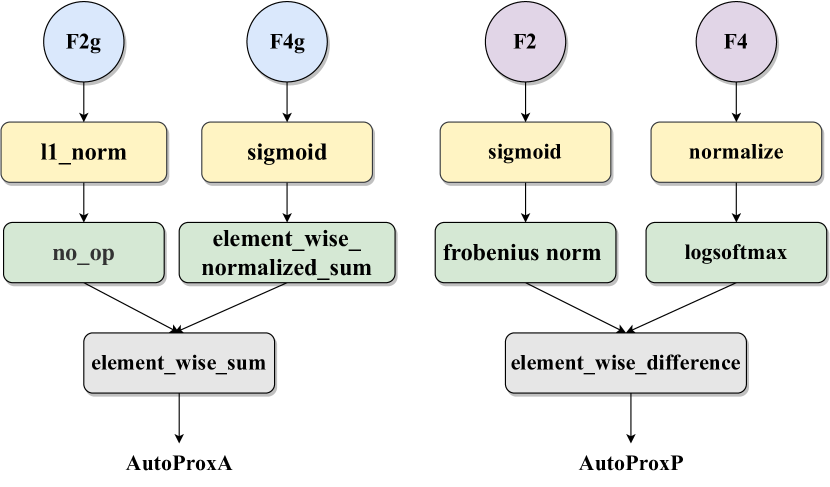
Figure 7: Illustration of searched zero-cost proxies on AutoFormer (Left) and PiT (Right) search spaces.

Appendix C Computation Graph Details

In Auto-Prox, each proxy within the population is encoded as a computation graph, comprising two inputs, a series of primitive operations, and a single output. For each input, there are eight possible selections (F1, F1g, F2, F2g, F3, F3g, F4, F4g). Additionally, there are 24 potential unary operations for processing each input, followed by four available binary operations to generate an output. The computation graph is designed to accept two types of network statistics as inputs, which can be either identical or distinct. For each branch of the computation graph, we apply two consecutive unary operations to transform the network statistics. Subsequently, we use a binary operation that takes the outputs of the two branches as input and applies the to_mean_scalar aggregation function to produce the final output. Figure 7 showcases the searched zero-cost proxies on Vision Transformers (ViTs) sampled from the AutoFormer and PiT search spaces.

Appendix D Validity Check for Zero-cost Proxies

We conduct a Validity Check for newly generated zero-cost proxies to reduce the number of invalid proxies during the search process. Specifically, we check if the proxy score of a proxy belongs to a set of invalid scores, which includes {-1, 1, 0, NaN, and Inf}. These scores indicate that the proxy is invalid and inapplicable.

Invalid proxy scores may manifest in several ways. For instance, a score of -1 could result from shape mismatch issues or user-defined exceptions, while a score of 1 may indicate a numerical insensitivity. A score of 0 may indicate a numerical instability or an invalid operation. The occurrence of NaN can be attributed to various factors, including division by zero, taking the square root of a negative number, or computing the logarithm of a non-positive number. A score of infinity (Inf) could be a result of overflow in arithmetic operations or arise from invalid mathematical operations.

We identify and filter out these invalid proxies after mutation, reducing the sparsity of the search space when seeking effective zero-cost proxies.

Appendix E More Experiments and Ablation Studies

Table 10: The effect of different seeds on the Kendall correlation results (%) of various zero-cost proxies. ViTs-accuracy configurations are sampled from the PiT search space and CIFAR-100 of ViT-Bench-101.

Proxy	random seed			AVG	STD
	0	1	2
GraSP	-49.32	-45.17	-31.56	-42.02	0.58
SynFlow	77.06	77.72	54.59	69.79	1.16
TE-NAS	4.08	-1.31	-9.17	-2.13	0.30
NWOT	-2.12	-2.18	-3.54	-2.61	0.01
TF-TAS	67.35	62.03	62.12	63.83	0.06
Auto-Prox (Ours)	86.19	86.04	73.98	82.07	0.33

Sensitivity Analysis of Seeds

To check the stability of various zero-cost proxies, we conduct experiments using three different seeds and compute the average and standard deviation. For each seed, we randomly sample 100 ViTs, then calculate the Kendall Tau correlation (%) between their distillation accuracy and corresponding zero-cost proxy scores. As shown in Table 10, Auto-Prox consistently achieves superior performance to other zero-cost proxies. These findings underscore the enhanced stability and reliability of our method in comparison to other alternative approaches.

Analysis of Iterations

In Figure 8, we provide an expanded view of the results from our evolutionary proxy search over a larger number of iterations. It can be observed that in the first 200 iterations, the evolutionary curve showed a clearly increasing trend. However, as the number of iterations continued to increase, only marginal improvements were achieved. Given these observations, and in pursuit of both computational efficiency and optimal performance, we have chosen to set the default number of evolutionary iterations at 200.

Training-free Search for Larger ViTs

We utilized the searched zero-cost proxy, denoted as AutoProxA, to conduct a training-free search for ViT models on AutoFormer-B (Chen et al. 2021a), within which the ViTs span a parameter range of approximately $42\sim 75$ M. Our goal is to explore the applicability and generality of our method for larger ViT models. In our experiments, we searched for 200 ViTs using different zero-cost proxies and reported the final distillation accuracy, model parameters, and search costs. As depicted in Table 11, our method can achieve even better results, suggesting that our method has the ability to adapt and generalize effectively to larger ViT models.

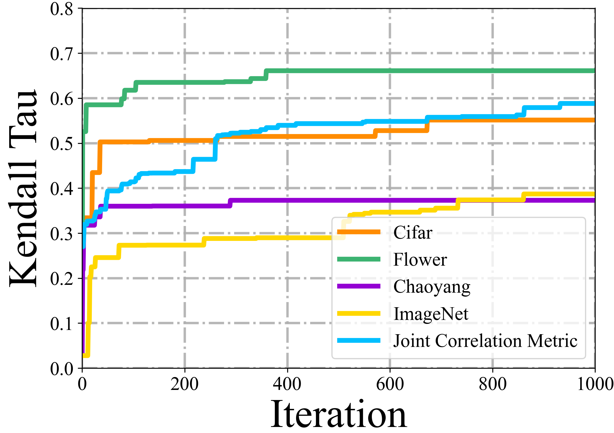
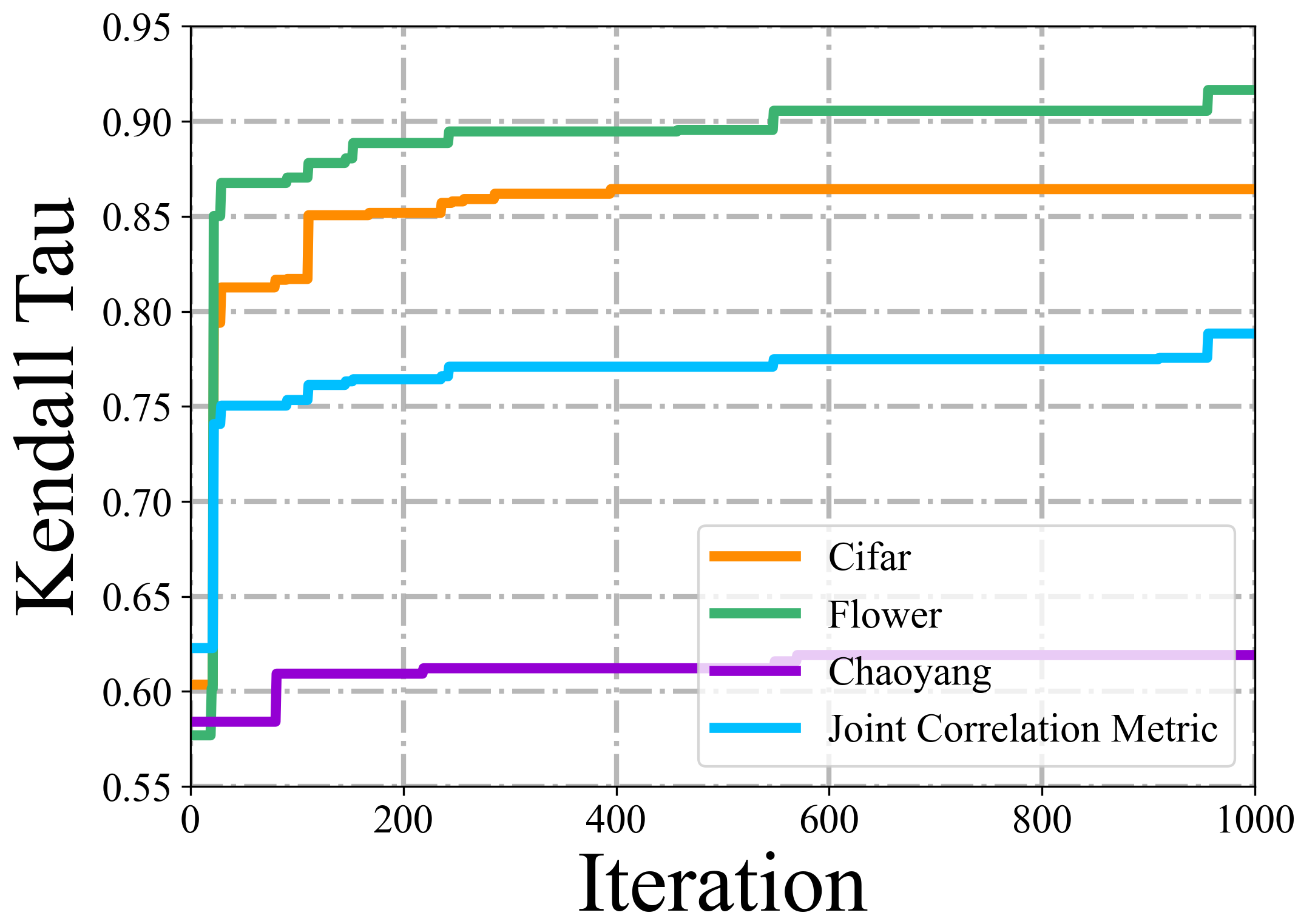
Figure 8: The 1000-iteration evolutionary processes of Kendall Tau on each dataset and the joint correlation metric. We search proxies for ViTs sampled from the AutoFormer search space (Left) and the PiT search space (Right).

Table 11: Training-free ViT search results using various zero-cost proxies in the AutoFormer-B search space. We report distillation accuracy on the CIFAR-100 dataset.

Search Space	Proxy	Param (M)	Search Cost	Dis. Acc(%)
AutoFormer-B	GraSP	68.94	1.79 h	80.22
	SynFlow	70.91	1.06 h	80.33
	TF-TAS	59.86	0.97 h	80.28
	Ours	52.22	0.55 h	80.51

Generalize to Other Architecture Search Space

To validate the generalization of Auto-Prox proxy to other architecture search space, we test the discovered AutoProxP on NAS-Bench-201 (Dong and Yang 2019). NAS-Bench-201 is a popular benchmark dataset that contains 15k unique CNN architectures. The results in Table 12 show that AutoProxP exhibits strong rank consistency, indicating its ability to generalize well to other architecture search spaces. We compare EZNAS-A (Akhauri et al. 2022) and AutoProxP in NAS-Bench-201. The results in Table 12 show that AutoProxP exhibits superior ranking consistency.

Table 12: Ranking correlation (%) on NAS-Bench-201 CIFAR-10. $\,{\dagger}$ means our implementation.

Proxy	Kendall	Spearman	Pearson
Snip	51.16	69.12	28.20
SynFlow	58.83	77.64	44.90
NWOT	55.13	74.93	84.18
EZNAS-A	65.00	83.00	-
EZNAS-A$\,{}^{\dagger}$	64.21	83.16	84.99
AutoProxP	68.49	84.81	86.71

Table 13: Searched architectures with Auto-Prox.

	Searched architectures
CIFAR-100
AutoFormer	{’mlp_ratio’: [3.5, 4.0, 3.5, 4.0, 3.5, 3.5, 4.0, 4.0, 4.0, 4.0, 4.0, 3.5, 4.0, 3.5], ’num_heads’: [4, 3, 3, 3, 4, 4, 4, 3, 4, 4, 4, 4, 3, 4], ’hidden_dim’: 240, ’depth’: 14}
PIT	{’mlp_ratio’: 6, ’num_heads’: [2, 2, 8], ’base_dim’: 32, ’depth’: [3, 4, 6]}
Flower
AutoFormer	{’mlp_ratio’: [3.5, 4.0, 4.0, 4.0, 4.0, 3.5, 4.0, 4.0, 4.0, 4.0, 4.0, 3.5, 4.0, 4.0], ’num_heads’: [4, 4, 3, 4, 4, 4, 3, 3, 4, 4, 4, 3, 3, 3], ’hidden_dim’: 240, ’depth’: 14}
PIT	{’mlp_ratio’: 8, ’num_heads’: [4, 4, 8], ’base_dim’: 32, ’depth’: [2, 8, 2]}
Chaoyang
AutoFormer	{’mlp_ratio’: [4.0, 4.0, 3.5, 4.0, 3.5, 4.0, 3.5, 4.0, 4.0, 4.0, 4.0, 3.5, 3.5], ’num_heads’: [3, 4, 4, 4, 3, 3, 3, 3, 4, 3, 4, 3, 3], ’hidden_dim’: 240, ’depth’: 13}
PIT	{’base_dim’:40, ’num_heads’: [2, 4, 4], ’mlp_ratio’: 6, ’depth’: [2, 4, 6]}
ImageNet
AutoFormer	{’mlp_ratio’: [3.5, 4.0, 4.0, 3.5, 3.5, 3.5, 3.5, 4.0, 4.0, 3.5, 3.5, 4.0, 3.5], ’num_heads’: [4, 4, 3, 4, 4, 3, 4, 4, 4, 3, 4, 3, 4], ’hidden_dim’: 192, ’depth’: 13}

Table 14: The unary and binary operations in the proxy search space. ”UOP” denotes the unary operation, and ”BOP” denotes the binary operation.

OP ID	OP Name	Input Args	Output Args	Description
UOP00	no_op	–	–	–
UOP01	element_wise_abs	$a$ / scalar,matrix	$b$ / scalar,matrix	$x_{b}=\left|x_{a}\right|$
UOP02	element_wise_tanh	$a$ / scalar,matrix	$b$ / scalar,matrix	$x_{b}=\tanh(x_{a})$
UOP03	element_wise_pow	$a$ / scalar,matrix	$b$ / scalar,matrix	$x_{b}=x_{a}^{2}$
UOP04	element_wise_exp	$a$ / scalar,matrix	$b$ / scalar,matrix	$x_{b}=e^{x_{a}}$
UOP05	element_wise_log	$a$ / scalar,matrix	$b$ / scalar,matrix	$x_{b}=\ln x_{a}$
UOP06	element_wise_relu	$a$ / scalar,matrix	$b$ / scalar,matrix	$x_{b}=\max(0,x_{a})$
UOP07	element_wise_leaky_relu	$a$ / scalar,matrix	$b$ / scalar,matrix	$x_{b}=\max(0.1x_{a},x_{a})$
UOP08	element_wise_swish	$a$ / scalar,matrix	$b$ / scalar,matrix	$x_{b}=x_{a}\times\text{sigmoid}(x_{a})$
UOP09	element_wise_mish	$a$ / scalar,matrix	$b$ / scalar,matrix	$x_{b}=x_{a}\times\text{tanh}(\ln{1+\text{exp}(x_{a})})$
UOP10	element_wise_invert	$a$ / scalar,matrix	$b$ / scalar,matrix	$x_{b}=1/x_{a}$
UOP11	element_wise_normalized_sum	$a$ / scalar,matrix	$b$ / scalar,matrix	$x_{b}=\frac{\sum x_{a}}{\text{numel}(x_{a})+\epsilon}$
UOP12	normalize	$a$ / scalar,matrix	$b$ / scalar,matrix	$x_{b}=\frac{x_{a}-\text{mean}(x_{a})}{\text{std}(x_{a})}$
UOP13	sigmoid	$a$ / scalar,matrix	$b$ / scalar,matrix	$x_{b}=\frac{1}{1+e^{-x_{a}}}$
UOP14	logsoftmax	$a$ / scalar,matrix	$b$ / scalar,matrix	$x_{b}=\ln\frac{e^{x_{a}}}{\sum_{i=1}^{n}e^{s_{i}}}$
UOP15	softmax	$a$ / scalar,matrix	$b$ / scalar,matrix	$x_{b}=\frac{e^{x_{a}}}{\sum_{i=1}^{n}e^{s_{i}}}$
UOP16	element_wise_sqrt	$a$ / scalar,matrix	$b$ / scalar,matrix	$x_{b}=\sqrt{x_{a}}$
UOP17	element_wise_revert	$a$ / scalar,matrix	$b$ / scalar,matrix	$x_{b}=-x_{a}$
UOP18	frobenius_norm	$a$ / scalar,matrix	$b$ / scalar,matrix	$x_{b}=\sqrt{\sum_{i=1}^{n}s_{i}^{2}}$
UOP19	element_wise_abslog	$a$ / scalar,matrix	$b$ / scalar,matrix	$x_{b}=\left|\ln x_{a}\right|$
UOP20	l1_norm	$a$ / scalar,matrix	$b$ / scalar,matrix	$x_{b}=\frac{\sum_{i=1}^{n}\left|s_{i}\right|}{\text{numel}(x_{a})}$
UOP21	min_max_normalize	$a$ / scalar,matrix	$b$ / scalar,matrix	$x_{b}=\frac{x_{a}-\min(x_{a})}{\max(x_{a})-\min(x_{a})}$
UOP22	to_mean_scalar	$a$ / scalar,matrix	$b$ / scalar	$x_{b}=\frac{x_{a}}{n}$
UOP23	to_std_scalar	$a$ / scalar,matrix	$b$ / scalar	$x_{b}=\sqrt{\frac{\sum_{i=1}^{n}(s_{i}-\bar{s})^{2}}{n}}$
BOP01	element_wise_sum	$a$,$b$ / scalar,matrixs	$c$ / scalar,matrix	$x_{c}=x_{a}+x_{b}$
BOP02	element_wise_difference	$a$,$b$ / scalar,matrixs	$c$ / scalar,matrix	$x_{c}=x_{a}-x_{b}$
BOP03	element_wise_product	$a$,$b$ / scalar,matrixs	$c$ / scalar,matrix	$x_{c}=x_{a}\times x_{b}$
BOP04	matrix_multiplication	$a$,$b$ / scalar,matrixs	$c$ / scalar,matrix	$x_{c}=x_{a}@x_{b}$

Appendix F Searched ViT with Auto-Prox

We provide details of searched architectures in the AutoFormer and PiT search spaces. These results can be found in Table 13. In the AutoFormer search space, the terms ”mlp_ratio” and ”num_heads” correspond to the values in all transformer layers. The ”hidden_dim” refers to the embedding dimension, while ”depth” denotes the number of transformer layers. Differently, the architectures within the PiT search space are stage-based. Both ”num_heads” and ”depth” have three values, each representing the result from the three distinct stages.

Appendix G Primitive Operations

The primitive operations utilized in Auto-Prox are classified into two categories based on their inputs. The unary operations are applied to a single input tensor, while the binary operations are conducted on two input tensors. The search space of the automatic proxy consists of 24 unary operations and 4 binary operations. Their detailed formulations are presented in Table 14.

References

- Abdi (2007) Abdi, H. 2007. The Kendall rank correlation coefficient. Encyclopedia of measurement and statistics, 2: 508–510.
- Akhauri et al. (2022) Akhauri, Y.; Munoz, J.; Jain, N.; and Iyer, R. 2022. EZNAS: Evolving Zero-Cost Proxies For Neural Architecture Scoring. Advances in Neural Information Processing Systems, 35: 30459–30470.
- Bowley (1928) Bowley, A. 1928. The standard deviation of the correlation coefficient. Journal of the American Statistical Association, 23(161): 31–34.
- Chen, Fan, and Panda (2021) Chen, C.-F. R.; Fan, Q.; and Panda, R. 2021. Crossvit: Cross-attention multi-scale vision transformer for image classification. In Proceedings of the IEEE/CVF International Conference on Computer Vision.
- Chen et al. (2022) Chen, K.; Yang, L.; Chen, Y.; Chen, K.; Xu, Y.; and Li, L. 2022. GP-NAS-ensemble: a model for the NAS Performance Prediction. In CVPRW.
- Chen et al. (2021a) Chen, M.; Peng, H.; Fu, J.; and Ling, H. 2021a. Autoformer: Searching transformers for visual recognition. In Proceedings of the IEEE/CVF International Conference on Computer Vision, 12270–12280.
- Chen et al. (2021b) Chen, M.; Peng, H.; Fu, J.; and Ling, H. 2021b. AutoFormer: Searching Transformers for Visual Recognition. In ICCV.
- Chen et al. (2021c) Chen, M.; Wu, K.; Ni, B.; Peng, H.; Liu, B.; Fu, J.; Chao, H.; and Ling, H. 2021c. Searching the Search Space of Vision Transformer. In Neural Information Processing Systems.
- Chen, Gong, and Wang (2020) Chen, W.; Gong, X.; and Wang, Z. 2020. Neural Architecture Search on ImageNet in Four GPU Hours: A Theoretically Inspired Perspective. In ICLR.
- Deng et al. (2009) Deng, J.; Dong, W.; Socher, R.; Li, L.-J.; Li, K.; and Fei-Fei, L. 2009. Imagenet: A large-scale hierarchical image database. In Proceedings of the IEEE/CVF Conference on Computer Vision and Pattern Recognition.
- Dong, Li, and Wei (2023) Dong, P.; Li, L.; and Wei, Z. 2023. Diswot: Student architecture search for distillation without training. In CVPR.
- Dong et al. (2023) Dong, P.; Li, L.; Wei, Z.; Niu, X.; Tian, Z.; and Pan, H. 2023. Emq: Evolving training-free proxies for automated mixed precision quantization. In Proceedings of the IEEE/CVF International Conference on Computer Vision, 17076–17086.
- Dong et al. (2022) Dong, P.; Niu, X.; Li, L.; Xie, L.; Zou, W.; Ye, T.; Wei, Z.; and Pan, H. 2022. Prior-Guided One-shot Neural Architecture Search. arXiv preprint arXiv:2206.13329.
- Dong et al. (2021) Dong, X.; Bao, J.; Chen, D.; Zhang, W.; Yu, N.; Yuan, L.; Chen, D.; and Guo, B. 2021. CSWin Transformer: A General Vision Transformer Backbone with Cross-Shaped Windows. ArXiv, abs/2107.00652.
- Dong and Yang (2019) Dong, X.; and Yang, Y. 2019. NAS-Bench-201: Extending the Scope of Reproducible Neural Architecture Search. In ICLR.
- Dong, Cordonnier, and Loukas (2021) Dong, Y.; Cordonnier, J.-B.; and Loukas, A. 2021. Attention is not all you need: Pure attention loses rank doubly exponentially with depth. In International Conference on Machine Learning, 2793–2803. PMLR.
- Dosovitskiy et al. (2020a) Dosovitskiy, A.; Beyer, L.; Kolesnikov, A.; Weissenborn, D.; Zhai, X.; Unterthiner, T.; Dehghani, M.; Minderer, M.; Heigold, G.; Gelly, S.; et al. 2020a. An image is worth 16x16 words: Transformers for image recognition at scale. arXiv preprint arXiv:2010.11929.
- Dosovitskiy et al. (2020b) Dosovitskiy, A.; Beyer, L.; Kolesnikov, A.; Weissenborn, D.; Zhai, X.; Unterthiner, T.; Dehghani, M.; Minderer, M.; Heigold, G.; Gelly, S.; et al. 2020b. An image is worth 16x16 words: Transformers for image recognition at scale. In ICLR.
- Han et al. (2021) Han, K.; Xiao, A.; Wu, E.; Guo, J.; Xu, C.; and Wang, Y. 2021. Transformer in transformer. Advances in Neural Information Processing Systems.
- Hu et al. (2021) Hu, Y.; Wang, X.; Li, L.; and Gu, Q. 2021. Improving one-shot NAS with shrinking-and-expanding supernet. Pattern Recognition.
- Jiang et al. (2021) Jiang, Z.-H.; Hou, Q.; Yuan, L.; Zhou, D.; Shi, Y.; Jin, X.; Wang, A.; and Feng, J. 2021. All tokens matter: Token labeling for training better vision transformers. Advances in Neural Information Processing Systems.
- Krizhevsky (2009) Krizhevsky, A. 2009. Learning multiple layers of features from tiny images. Technical report.
- Krizhevsky and Hinton (2009) Krizhevsky, A.; and Hinton, G. 2009. Learning multiple layers of features from tiny images. Tech Report.
- Krizhevsky et al. (2009) Krizhevsky, A.; et al. 2009. Learning multiple layers of features from tiny images. Technical report, Citeseer.
- Lee, Ajanthan, and Torr (2018) Lee, N.; Ajanthan, T.; and Torr, P. H. 2018. Snip: Single-shot network pruning based on connection sensitivity. arXiv preprint arXiv:1810.02340.
- Li et al. (2021a) Li, C.; Tang, T.; Wang, G.; Peng, J.; Wang, B.; Liang, X.; and Chang, X. 2021a. BossNAS: Exploring Hybrid CNN-transformers with Block-wisely Self-supervised Neural Architecture Search. 2021 IEEE/CVF International Conference on Computer Vision (ICCV), 12261–12271.
- Li et al. (2022a) Li, H.; Fu, T.; Dai, J.; Li, H.; Huang, G.; and Zhu, X. 2022a. Autoloss-zero: Searching loss functions from scratch for generic tasks. In Proceedings of the IEEE/CVF Conference on Computer Vision and Pattern Recognition, 1009–1018.
- Li et al. (2022b) Li, K.; Yu, R.; Wang, Z.; Yuan, L.; Song, G.; and Chen, J. 2022b. Locality guidance for improving vision transformers on tiny datasets. In European Conference on Computer Vision, 110–127. Springer.
- Li (2022) Li, L. 2022. Self-Regulated Feature Learning via Teacher-free Feature Distillation. In ECCV.
- Li et al. (2023a) Li, L.; Dong, P.; Li, A.; Wei, Z.; and Ya, Y. 2023a. KD-Zero: Evolving Knowledge Distiller for Any Teacher-Student Pairs. In Thirty-seventh Conference on Neural Information Processing Systems.
- Li et al. (2023b) Li, L.; Dong, P.; Wei, Z.; and Yang, Y. 2023b. Automated Knowledge Distillation via Monte Carlo Tree Search. In ICCV.
- Li and Jin (2022) Li, L.; and Jin, Z. 2022. Shadow knowledge distillation: Bridging offline and online knowledge transfer. Advances in Neural Information Processing Systems.
- Li et al. (2022c) Li, L.; Shiuan-Ni, L.; Yang, Y.; and Jin, Z. 2022c. Boosting Online Feature Transfer via Separable Feature Fusion. In IJCNN.
- Li et al. (2022d) Li, L.; Shiuan-Ni, L.; Yang, Y.; and Jin, Z. 2022d. Teacher-free Distillation via Regularizing Intermediate Representation. In IJCNN.
- Li et al. (2021b) Li, Y.; Zhang, K.; Cao, J.; Timofte, R.; and Gool, L. V. 2021b. LocalViT: Bringing Locality to Vision Transformers. ArXiv, abs/2104.05707.
- Liang et al. (2022) Liang, Y.; GE, C.; Tong, Z.; Song, Y.; Wang, J.; and Xie, P. 2022. EViT: Expediting Vision Transformers via Token Reorganizations. In International Conference on Learning Representations.
- Liu et al. (2021a) Liu, S.; Ni’mah, I.; Menkovski, V.; Mocanu, D. C.; and Pechenizkiy, M. 2021a. Efficient and effective training of sparse recurrent neural networks. Neural Computing and Applications, 1–12.
- Liu et al. (2023) Liu, X.; Li, L.; Li, C.; and Yao, A. 2023. NORM: Knowledge Distillation via N-to-One Representation Matching. arXiv preprint arXiv:2305.13803.
- Liu et al. (2021b) Liu, Z.; Lin, Y.; Cao, Y.; Hu, H.; Wei, Y.; Zhang, Z.; Lin, S.; and Guo, B. 2021b. Swin transformer: Hierarchical vision transformer using shifted windows. In Proceedings of the IEEE/CVF International Conference on Computer Vision.
- Loshchilov and Hutter (2016) Loshchilov, I.; and Hutter, F. 2016. Sgdr: Stochastic gradient descent with warm restarts. arXiv preprint arXiv:1608.03983.
- Loshchilov and Hutter (2017) Loshchilov, I.; and Hutter, F. 2017. Decoupled Weight Decay Regularization. In International Conference on Learning Representations.
- Lu et al. (2024) Lu, L.; CHen, Z.; Lu, L., Xiaoyu; Rao, Y.; Li, L.; and Pang, S. 2024. UniADS: Universal Architecture-Distiller Search for Distillation Gap. In AAAI.
- Mellor et al. (2021) Mellor, J.; Turner, J.; Storkey, A.; and Crowley, E. J. 2021. Neural architecture search without training. In ICML.
- Mozer and Smolensky (1988) Mozer, M. C.; and Smolensky, P. 1988. Skeletonization: A Technique for Trimming the Fat from a Network via Relevance Assessment. In NIPS.
- Nilsback and Zisserman (2008) Nilsback, M.-E.; and Zisserman, A. 2008. Automated flower classification over a large number of classes. In 2008 Sixth Indian Conference on Computer Vision, Graphics & Image Processing, 722–729. IEEE.
- Real et al. (2020) Real, E.; Liang, C.; So, D. R.; and Le, Q. V. 2020. AutoML-Zero: Evolving Machine Learning Algorithms From Scratch. arXiv:2003.03384.
- Shao et al. (2023) Shao, S.; Dai, X.; Yin, S.; Li, L.; Chen, H.; and Hu, Y. 2023. Catch-Up Distillation: You Only Need to Train Once for Accelerating Sampling. arXiv preprint arXiv:2305.10769.
- Stephanou and Varughese (2021) Stephanou, M.; and Varughese, M. 2021. Sequential estimation of Spearman rank correlation using Hermite series estimators. Journal of Multivariate Analysis, 186: 104783.
- Su et al. (2021a) Su, X.; You, S.; Xie, J.; Zheng, M.; Wang, F.; Qian, C.; Zhang, C.; Wang, X.; and Xu, C. 2021a. Vision Transformer Architecture Search. arXiv preprint arXiv:2106.13700.
- Su et al. (2021b) Su, X.; You, S.; Xie, J.; Zheng, M.; Wang, F.; Qian, C.; Zhang, C.; Wang, X.; and Xu, C. 2021b. ViTAS: Vision Transformer Architecture Search. In European Conference on Computer Vision.
- Tanaka et al. (2020) Tanaka, H.; Kunin, D.; Yamins, D. L.; and Ganguli, S. 2020. Pruning neural networks without any data by iteratively conserving synaptic flow. NeurIPS.
- Theis et al. (2018) Theis, L.; Korshunova, I.; Tejani, A.; and Huszár, F. 2018. Faster gaze prediction with dense networks and Fisher pruning. ArXiv, abs/1801.05787.
- Touvron et al. (2021) Touvron, H.; Cord, M.; Douze, M.; Massa, F.; Sablayrolles, A.; and Jégou, H. 2021. Training data-efficient image transformers & distillation through attention. In ICML. PMLR.
- Wang et al. (2021) Wang, W.; Xie, E.; Li, X.; Fan, D.-P.; Song, K.; Liang, D.; Lu, T.; Luo, P.; and Shao, L. 2021. Pyramid Vision Transformer: A Versatile Backbone for Dense Prediction without Convolutions. In ICCV.
- Wei et al. (2023) Wei, Z.; Pan, H.; Li, L.; Dong, P.; Tian, Z.; Niu, X.; and Li, D. 2023. TVT: Training-Free Vision Transformer Search on Tiny Datasets. arXiv preprint arXiv:2311.14337.
- Wu et al. (2022) Wu, K.; Zhang, J.; Peng, H.; Liu, M.; Xiao, B.; Fu, J.; and Yuan, L. 2022. TinyViT: Fast Pretraining Distillation for Small Vision Transformers. ArXiv, abs/2207.10666.
- Xie et al. (2019) Xie, S.; Zheng, H.; Liu, C.; and Lin, L. 2019. SNAS: stochastic neural architecture search. In ICLR.
- Zhou et al. (2022) Zhou, Q.; Sheng, K.; Zheng, X.; Li, K.; Sun, X.; Tian, Y.; Chen, J.; and Ji, R. 2022. Training-free Transformer Architecture Search. In Proceedings of the IEEE/CVF Conference on Computer Vision and Pattern Recognition, 10894–10903.
- Zhu et al. (2021) Zhu, C.; Chen, W.; Peng, T.; Wang, Y.; and Jin, M. 2021. Hard Sample Aware Noise Robust Learning for Histopathology Image Classification. IEEE Transactions on Medical Imaging, 41(4): 881–894.
- Zimian Wei et al. (2024) Zimian Wei, Z.; Li, L. L.; Dong, P.; Hui, Z.; Li, A.; Lu, M.; Pan, H.; and Li, D. 2024. Auto-Prox: Training-Free Vision Transformer Architecture Search via Automatic Proxy Discovery. In AAAI.