A Sparse Cross Attention-based Graph Convolution Network with Auxiliary Information Awareness for Traffic Flow Prediction

Abstract

Deep graph convolution networks (GCNs) have recently shown excellent performance in traffic prediction tasks. However, they face some challenges. First, few existing models consider the influence of auxiliary information, i.e., weather and holidays, which may result in a poor grasp of spatial-temporal dynamics of traffic data. Second, both the construction of a dynamic adjacent matrix and regular graph convolution operations have quadratic computation complexity, which restricts the scalability of GCN-based models. To address such challenges, this work proposes a deep encoder-decoder model entitled AIMSAN. It contains an auxiliary information-aware module (AIM) and sparse cross attention-based graph convolution network (SAN). The former learns multi-attribute auxiliary information and obtains its embedded presentation of different time-window sizes. The latter uses a cross-attention mechanism to construct dynamic adjacent matrices by fusing traffic data and embedded auxiliary data. Then, SAN applies diffusion GCN on traffic data to mine rich spatial-temporal dynamics. Furthermore, AIMSAN considers and uses the spatial sparseness of traffic nodes to reduce the quadratic computation complexity. Experimental results on three public traffic datasets demonstrate that the proposed method outperforms other counterparts in terms of various performance indices. Specifically, the proposed method has competitive performance with the state-of-the-art algorithms but saves 35.74% of GPU memory usage, 42.25% of training time, and 45.51% of validation time on average.

I Introduction

The increasing use of vehicles makes the city’s transportation-related problems increasingly severe, like traffic jams and air pollution [1, 2]. Therefore, research on traffic flow has attracted wide attention, among which traffic data prediction is one hot spot. However, traffic flow has complex spatial-temporal dynamics influenced by human activities and other factors (like weather). For example, due to people commuting to work, the traffic flow in the morning or evening rush hour is significantly higher than that in other periods on the same day. The traffic speed during foggy days is slower than that during clear days. Besides, those road repairs or accidental traffic events cause unexpected traffic jams on certain roads.

In recent years, deep learning models have been widely used to solve traffic prediction tasks thanks to their remarkable representational ability, among which spatial-temporal models are the most promising ones [3, 4]. In the early research stage, dividing the distributions of traffic states into grids on a map, the studies in [5, 6] apply convolution neural networks (CNN) to extract spatial interactions and adopt recurrent neural networks (RNN) to learn temporal dependency. However, considering the natural graph structure of traffic sensors, more researchers have found that it is more reasonable to mine the spatial interactions of traffic data in the form of graph diffusion [7, 8]. Given the traffic data by a graph structure, Fig. 1 shows the traffic states update process after one graph convolution network (GCN) operation, where $X_{\text{n1}}$ is the current data state of node 1 ($n_{1}$), $X_{\text{n1}}^{\prime}$ is the updated state, and $w_{i,j}$ is the weight between $n_{i}$ and $n_{j}$. In GCN, each node updates local traffic states by weighting the data from itself and its neighbors.

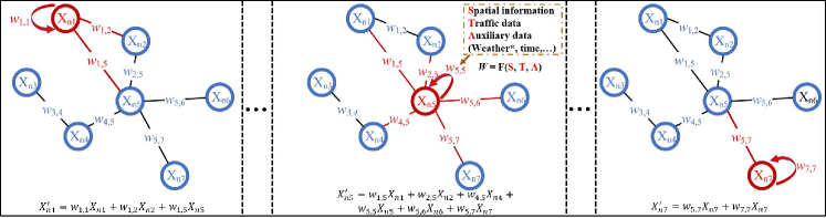
Figure 1: Traffic states update process under one GCN operation.

Recently, most researchers have focused on graph convolution, especially dynamic graph convolution. Those dynamic methods mainly apply specific mechanisms to calculate variable weights of adjacency matrices in each GCN process and then use the new adjacency matrices to update the traffic states. For example, Han et al. in [9] design a dynamic graph constructor to generate a time-specific adjacency tensor. As a result, those GCN models can learn more hidden spatial-temporal information with dynamic graph convolution operation.

However, two key issues remain to be investigated for GCN-based models. First, traffic data contain complex spatial-temporal dynamics influenced by traffic attributes and other factors like weather and holidays. Yet, many graph convolution models adopt the same graph for information extraction under all conditions, whether using static graphs (based on distance) or self-adaptive ones (based on learning), which ignores the spatial-temporal diversity of traffic data [4]. Even for those dynamic GCN models [10, 11], few existing studies consider the influence of auxiliary information. Those auxiliary information are non-negligible because they can help the model learn more about hidden traffic states. Therefore, in GCN operations shown in Fig. 1, AIMSAN considers designing a fusion function F(S, T, A) to embed spatial information, traffic data, and auxiliary information (like weather and holiday) for constructing an auxiliary-information-aware dynamic adjacent matrix, which can be used to mine rich spatial-temporal dynamics. Second, with the expansion of a city, the scalability of GCN-based models is restricted by the traffic node size ($N$) due to the quadratic computation complexity of regular graph convolution operations.

This paper presents a deep encoder-decoder model called AIMSAN containing Dilated Causal Convolution network (DCC), AIM and SAN modules to address the above two issues. DCC is a temporal convolutional network that can reduce the stacking layer size by dilation convolutions. AIM can embed multiple-attribute auxiliary information in the historical or future periods into one tensor representation. The historical embedded data are fed into SAN, and future embedded data are added to the decoder part to increase the model’s awareness of future auxiliary information. In each encoder layer, AIMSAN concatenates feed-forward data with the embedded data to calculate the dynamic adjacent matrix using a cross-attention mechanism. Subsequently, it uses dynamic adjacent matrices to mine rich spatial-temporal information from traffic data. In short, this work intends to make the following novel contributions to the field of traffic prediction:

1) It proposes an auxiliary information-aware method to embed multiple attributes like time, position, and weather conditions and learn more about hidden traffic states. In the encoder layer, AIM aligns the historical auxiliary data with hidden traffic data in the temporal dimension to keep its focus on the information in the current time window. Besides, AIM embeds future auxiliary data in the decoder to improve its understanding of the predicted traffic state. Lastly, AIM is easy to be trimmed and extended due to its multi-branch structure.

2) It designs a novel dynamic adjacency matrix acquisition method that fuses traffic data and embedded data from AIM to obtain an auxiliary-information-aware dynamic adjacency matrix and mines rich spatial-temporal diversity for the first time.

3) It proposes a sparse cross-attention-based graph convolution (SAN) module that applies the spatial sparseness of traffic nodes to a graph convolution process, thus reducing the computational complexity.

4) It evaluates the proposed approach and existing state-of-the-art ones on three real-world datasets. Experimental results demonstrate that it outperforms its peers in most cases.

The rest of this paper is organized as follows: Section ii@ introduces the related work about traffic flow prediction. Then, Section iii@ gives the problem statement of traffic prediction. Section iv@ describes the implementation of AIMSAN. Section v@ presents the experimental results and discussions. Finally, Section vi@ concludes this work.

II Related work

Deep learning methods have been widely used for traffic prediction. This section introduces some deep traffic prediction models with or without GCN.

II-A Traffic prediction without GCN

Those traffic prediction models without GCN are mainly based on Stacked Autoencoder (SAE), Deep Belief Networks (DBN), Recurrent Neural Networks (RNN), Convolutional Neural Networks (CNN), or hybrid ones [12]. In the early stage, some studies consider optimizing the computation time of training models. Therefore, they apply SAEs and DBNs in traffic flow prediction [13, 14, 15]. However, many researchers verify that they fail to capture the spatial or temporal aspect of the traffic data and thus tend to perform worse than those spatial-temporal-correlation-based neural networks [16]. Differently, RNN-based models are naturally suitable for traffic time-series data mining. For example, Fouladgar et al. in [17] constructed the traffic data as a matrix and used an LSTM to capture the hidden spatial-temporal correlation of data. However, with the growth of the traffic flow prediction series, those RNN-based models require long input sequences, which can heavily impact the training and inference efficiency.

CNN is another optional deep-learning framework for traffic prediction tasks thanks to its ability to capture the correlation between different regions or time slots. Like RNNs, the temporal convolutional network (TCN) is a typical 1D CNN model that can be used to analyze traffic data from the temporal dimension. Considering the spatial-temporal attributes of traffic data, some CNN-based models perform 2D CNN on traffic data in both temporal and spatial dimensions [17], like an image feature extraction process [18, 19].

In addition, hybrid models have been extensively studied because they can utilize the strengths of their individual components. For example, Du et al. [20] combine both CNN and LSTM components to capture spatial and temporal features, respectively, and fuse the outputs from the above two networks to form the final prediction. Another version of hybrid methods adds convolutional operation into the dense kernel of the LSTM unit such that the improved LSTM model can simultaneously capture the spatial-temporal correlation of traffic data. Though CNNs can efficiently mine the spatial patterns of traffic data, most of them regard the spatial relationship of traffic flow as a simple Euclidean structure while ignoring the complex spatial relationship among nodes. Thus 2D CNN is not the best choice for the prediction of graph structure traffic data.

II-B Traffic prediction with GCN

The graph convolution network (GCN) [21, 22, 23] is an effective method for data extraction, especially for those data with graph structures like traffic data. Unlike 2D CNN, a GCN model learns the transformation of traffic data through graph diffusion. GCN models are roughly divided into two groups: traditional and dynamic ones.

Traditional GCN models apply a fixed adjacent matrix in each graph convolution layer [24, 7, 8]. For example, in [8], the authors use both static and learnable adjacent matrices, where the weights of a static adjacent matrix are initialized according to the distance between each pair of traffic nodes, and the learnable adjacent matrix is constructed by the matrix multiplication of two embedding matrices. However, whether using predefined adjacent matrices (like distance-based or content-based adjacent matrices) or learnable ones, those adjacent matrices are fixed once a model is trained, thus ignoring the sample and position-specific characteristics of data [25].

Dynamic GCNs are increasingly being applied for traffic prediction tasks, which construct variable adjacency matrices to mine the rich spatial-temporal information [10, 11]. Considering the daily periodicity of traffic status, the Dynamic and Multi-faceted Spatio-Temporal Graph Convolution Network (DMSTGCN) in [9] uses an inverse process of Tucker decomposition to construct a dynamic adjacent matrix $\mathbf{A}\in\mathbb{R}^{N_{t}\times N\times N}$, where $N_{t}$ is the number of time slots in a day. Therefore, DMSTGCN can learn the time-specific spatial dependencies of road segments. Besides, it applies a dynamic graph convolution module to aggregate the hidden states of neighbor nodes to focal nodes by passing messages on the dynamic adjacency matrices. Differently, Li et al. [10] propose a spatial-temporal fusion graph neural network (STFGNN). They use a data-driven method to generate a dynamic adjacent matrix of size $N\times N$. By combining multiple spatial and temporal graphs, STFGNN can efficiently learn the spatial-temporal correlations simultaneously. However, stacking adjacent matrices of size $4N\times 4N$ in STFGNN dramatically increases computation and memory costs. In addition, attention-based graph neural networks are used to model the spatial-temporal dynamic of traffic data [26, 27]. For example, Guo et al. [26] design a self-attention module to capture temporal dynamics of traffic data and use a dynamic graph convolution module to learn spatial correlations. Dynamic GCN models can discover more hidden correlations than traditional GCN models. However, they only use traffic data (like traffic speed or flow) and ignore the influence of auxiliary factors.

Several methods have recently utilized auxiliary information of road segments, like speed limit, joint angle, and points of interest, to mine the hidden feature of traffic data [28, 29, 4]. For example, Shin et al. [28] propose a multi-weight traffic graph convolutional network (MW-TGC). They conduct graph convolution operations on speed data with multi-weighted adjacency matrices to combine the auxiliary features, including speed limit, distance, and angle. In [9], the authors explore dynamic and multi-faceted spatial-temporal characteristics inherent in traffic data and use traffic volumes to predict future traffic speed. In addition, Pan et al. [30] propose a meta-learning-based mode named ST-MetaNet, which applies meta-knowledge learners to learn the edge and node attributes of traffic sensors and uses the learned weights to construct a dynamic adjacent matrix to mine spatial-temporal information. Unlike ST-MetaNet, AIMSAN uses a cross-attention strategy to construct a dynamic adjacent matrix, which fuses traffic state data with multiple attribute data like positional, temporal and weather information in historical and future periods.

The most related work to this paper is our previous work (TGANet) in [27]. TGANet is a dynamic graph convolutional method that uses self-attention-based and multi-weight adjacent matrices to mine spatial-temporal dynamics of traffic data. However, it has the following deficiencies. First, like many dynamic GCN methods, TGANet neglects the influence of auxiliary factors like weather toward the target attribute. Second, the multi-weight GCN operation in TGANet requires extra computation costs. Unlike it, AIMSAN designs AIMs for learning the sample and position-specific auxiliary information and constructs an auxiliary information-aware adjacent matrix to learn rich spatial-temporal dynamics. Only using the auxiliary information-aware adjacent matrix, AIMSAN requires less computation overhead than TGANet.

III Problem statement

In intelligent traffic systems, traffic monitoring nodes (called nodes for short) are usually deployed around the city, as shown in Fig. 2(a). The distribution of such nodes forms a graph structure $G=\{\mathbf{V},\mathbf{E}\}$ like Fig. 2(b), where $\mathbf{V}=\{v_{1},v_{2},\cdots,v_{n}\}$ is the set of nodes, and $\mathbf{E}$ is the set of edges. In addition, the adjacency matrix $\mathbf{A}=[a_{ij}]\in\mathbb{R}^{N\times N}$ records the connection between each pair of nodes. If nodes $v_{i}$ and $v_{j}$ belong to $\mathbf{V}$, and they are connected, then $e_{ij}\in\mathbf{E}$, and $a_{ij}=1$. If not connected, $a_{ij}=0$.

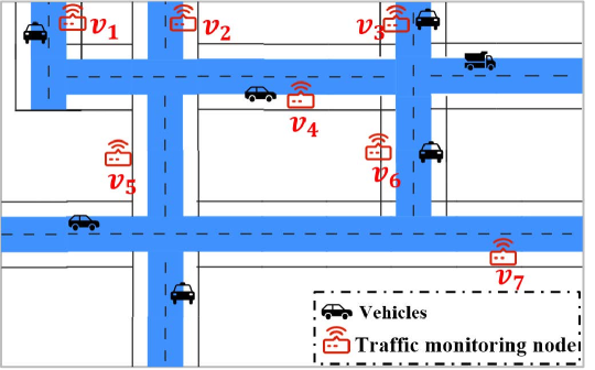
(a) Urban area

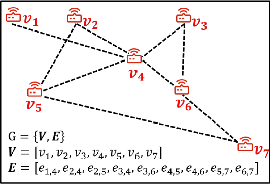
(b) Graph structure

Figure 2: An example of traffic sensor node distribution in a city.

TABLE I: Frequently used notations

Notation	Description	Notation	Description
G={$\mathbf{V}$, $\mathbf{E}$}	A graph structure, where $\mathbf{V}$ is the set of nodes, $\mathbf{E}$ is the set of edges	$\mathbf{I}_{j}$/$\mathbf{S}_{j}$	Input data and skip data in the $j^{\text{th}}$ SAN Layer
$\mathbf{A}$/$\mathbf{A}_{N}$/$\mathbf{A}^{b}$	An adjacent matrix/normalized adjacent matrix/ the $b^{\operatorname{th}}$ adjacent matrix of the batch adjacent matrices in SAN layer	$\mathbf{Q}$/$\mathbf{K}$/$\mathbf{V}$	Query/Key/Value of an attention module
$\mathbb{N}$/$\mathbb{S}$/$\mathbb{T}$	A node index set/sampling time-slots set of input data/ sampling time-slots set of predicting data	$\mathbf{M}$/$\mathcal{D}$/$\mathcal{I}$	Mask matrix/degree matrix/identity matrix
$N$/$S$/$T$	Node size/sequence length of input data/sequence length of target data	$h$	Head size of multi-attention module
$\mathbf{X}$/$\mathbf{Y}$/$\mathbf{D}$/$\mathbf{F}$	Input data/target data/historical auxiliary factors/ future auxiliary factors	$q$/$p$	Dimension of input data/auxiliary factors

This paper focuses on performing long sequence time-series forecasting tasks on point traffic data. Let a node index set be $\mathbb{N}=\{1,2,\cdots,N\}$, the sampling time-slots of input historical data at time $t$ be $\mathbb{S}=\{t-S+1,t-S+2,\cdots,t\}$, and the sampling time-slots of predicting data be $\mathbb{T}=\{t+1,\cdots,t+T\}$, where $S$ is the input sequence length and $T$ is predicting sequence length. The traffic data of node $i$ sampled at time $t$ is $X_{i}^{(t)}=<x_{i,1}^{(t)},\cdots,x_{i,q}^{(t)}>\in R^{q}$, which contains $q$ traffic attributes like traffic speed and traffic volume. Therefore, the historical traffic data can be represented by $\mathbf{X}={\{X_{i}^{(t)}|i\in\mathbb{N}\}}_{t\in\mathbb{S}}$ and future traffic data can be represented by $\mathbf{Y}={\{X_{i}^{(t)}|i\in\mathbb{N}\}}_{t\in\mathbb{T}}$. In addition, some auxiliary attributes like sampling time, positional information, and weather states are absorbed to mine rich spatial-temporal correlation. Let the auxiliary attributes of node $i$ sampled at time $t$ be $D_{i}^{(t)}=<d_{i,1}^{(t)},\cdots,d_{i,p}^{(t)}>\in R^{p}$, which contains $p$ attributes. According to different sampling time, the auxiliary data can be divided into historical auxiliary data $\mathbf{D}={\{D_{i}^{(t)}|i\in\mathbb{N}\}}_{t\in\mathbb{S}}$ and future auxiliary data $\mathbf{F}={\{D_{i}^{(t)}|i\in\mathbb{N}\}}_{t\in\mathbb{T}}$.

Therefore, we can express the traffic data forecasting tasks: $f:\mathbf{X}\times\mathbf{D}\times\mathbf{F}\times\mathbf{G}\rightarrow\mathbf{Y}$ . In the form of a sliding window, those historical data of $S$ time-slots including traffic data $\mathbf{X}$, historical auxiliary data $\mathbf{D}$, future auxiliary data $\mathbf{F}$ and the graph structure $\mathbf{G}$ are fed into the forecasting model $f$ to produce the traffic states $\mathbf{Y}$ in the next $T$ time-slots.

For better understanding, frequently used notations are listed in Table I.

IV Proposed method

As shown in Fig. 3, AIMSAN is an encoder-decoder model, mainly including two modules, i.e. AIM and SAN. It uses the historical traffic data $\mathbf{X}$, historical auxiliary data $\mathbf{D}$ and future auxiliary data $\mathbf{F}$ to train its model, producing the predictions of future traffic data $\mathbf{Y}$.

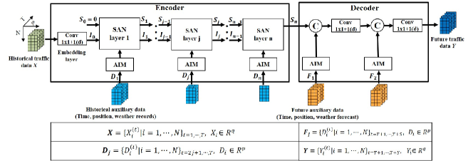
Figure 3: Framework of AIMSAN.

IV-A Encoder structure

Our encoder includes one embedding layer, $n$ AIMs and $n$ SAN layers. Specifically, historical traffic data $\mathbf{X}$ is fed into the embedding layer to increase the attribute dimension, where ”Conv 1x1+1(d)” stands for 1x1 convolutions with the dilation as 1. Due to the use of dilated causal convolution, the temporal dimension of hidden data in each SAN module decreases with each layer. The historical auxiliary data are fed into AIM to learn the sample and position-specific external influence. The temporal dimensions of historical auxiliary data are consistent with those of hidden data in the corresponding SAN layers. Then the ${(j-1)}^{th}$ layer output data $\mathbf{I_{j-1}}$, the feed-forward data of skip connection (i.e. skip data) $\mathbf{S_{j-1}}$ and AIM output $\mathbf{D_{j}}$ are fed into the $j^{\operatorname{th}}$ SAN layer with two outputs, $\mathbf{S_{j}}$ and $\mathbf{I_{j}}$. Skip data $\mathbf{S_{j}}$ contain the hidden presentation of the foregoing layers, which are initiated to zeros and accumulated in each SAN layer. The AIM and SAN modules are elaborated next.

IV-A1 AIM

Traffic data is influenced by many auxiliary factors, like time (time of day, day of week, and holiday), position (longitude and latitude, or POI), and weather conditions. Therefore, AIMSAN applies AIM to analyze the influence of auxiliary factors. The produced weights are concatenated with hidden data in the following attention module by which AIMSAN can learn auxiliary information-aware attention values and mine more spatiotemporal dependencies of traffic data. Fig. 4 shows the structure of AIM, where the sampling time information, corresponding weather conditions, and node positions are fed into three independent embedding branches. Each branch is constructed by two fully-connected layers. Subsequently, the outputs of three branches are concatenated into one tensor $\mathbf{D_{j}}=[N,T^{\prime},3H]$ using matrix expansion and concatenation operations, where $N$ is the node size, $T^{\prime}$ is the time-series length, and $H$ is the dimension of hidden layer. Due to the lack of POI information, positional attributes only consist of latitude and longitude values in this paper. Future weather information can be obtained from weather forecast data in practice. Thanks to the branch structure of AIM, we can tailor it to only mine temporal information for those open-source datasets without any positional information. In addition, it is easy to add new auxiliary factors into AIM.

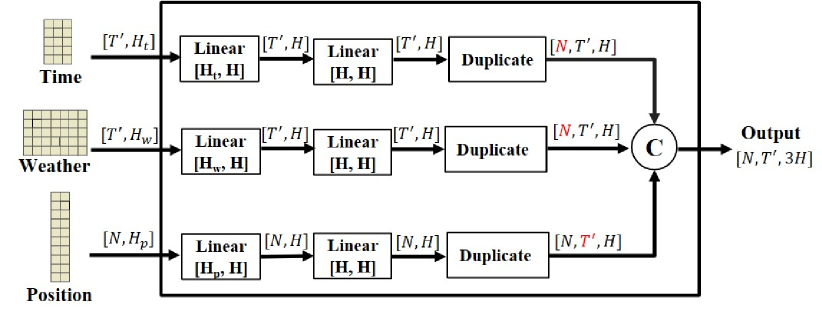
Figure 4: The structure of an AIM, where C denotes a concatenation operation.

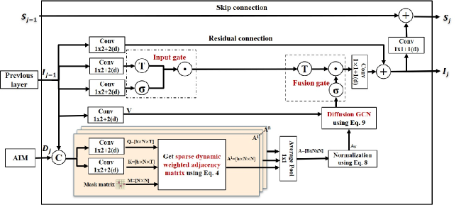
Figure 5: Frameworks of sparse cross attention-based diffusion GCN (SAN) layer.

IV-A2 SAN layer

Fig. 5 shows the framework of SAN. It takes the previous layer output $\textbf{I}_{j-1}$, $j^{\operatorname{th}}$ AIM output $\textbf{D}_{j}$ and skip data $\textbf{S}_{j-1}$ as inputs and produces the layer output $\textbf{I}_{j}$ and accumulated $\textbf{S}_{j}$. The SAN layer mainly includes a DCC module, sparse attention graph convolution module and two gate structures (input gate and fusion gate).

DCC: First, we introduce the DCC module used in the SAN layer. It is used to mine temporal dependency and reduce the temporal dimension of hidden data, where ”Conv 1x2+2(d)” stands for 1x2 convolutions with the dilation as 2. Unlike the step-by-step manner in RNN, DCC enlarges its receptive field by stacking the network layers, which can improve the propagation efficiency and avoid the potential gradient problem in RNN-based models.

AIMSAN applies DCC in each SAN layer to learn the temporal dependency and slim its model size. Taking the input temporal dimension $T=12$ and dilation factors [2, 2, 2, 2, 2, 1] for example, Fig. 6 shows the function of a DCC structure in the reduction dimension by ignoring the other modules in AIMSAN. Formally, given a 1-D sequence input $X\in\mathbb{R}^{T}$ and a filter $f\in\mathbb{R}^{k}$, the dilated convolution operation of $X$ with $f$ at step $t$ can be represented as:

$$X\ast f(t)=\sum_{i=0}^{k-1}f(i)\cdot X(t-d\times i),$$ (1)

where $\ast$ denotes the convolution operation, $d$ represents the dilation factor, $k$ represents the size of the filter, and the numbers in parenthesis ($t-d\times i$) indicate the indices of the vectors. When $d=1$, dilation convolution is equivalent to common causal convolution. As shown in Fig. 6, the temporal dimensions of those feed-forward data are reduced gradually after each DCC, and finally converge to 1. Therefore, the feed-forward data in the last SAN layer contain all the temporal information in the past $T$ time slots.

Figure 6: Framework of dilated causal convolution structure, taking the input temporal dimension $T$=12 and dilation factors as [2, 2, 2, 2, 2, 1] as an example.

GCN operations: Inspired by the weighted matrix in the cross-attention module of Transformer [31], AIMSAN calculates the auxiliary-information-aware weighted matrix as the adaptive adjacent matrix for the graph convolution operation.

$$\mathbf{I}_{j}^{\prime}=\mathbf{I}_{j}\;||\;\mathbf{D}_{j+1}$$ (2)

$$\mathbf{A}^{b}=FF(\mathbf{I}_{j}^{\prime})\times FF(\mathbf{I}_{j}^{\prime})^{T},\;\mathbf{A}^{b}\in\mathbb{R}^{N\times N}$$ (3)

In (2), AIMSAN concatenates the output of the $j^{th}$ SAN layer $\textbf{I}_{j}$ with historical embedded auxiliary information $\textbf{D}_{j+1}$ in node size dimension, where $||$ is vector concatenation operator, and $\textbf{I}_{j}^{\prime}$ is the results. The calculation process of the attention-based weighted matrix is shown in (3), where the FF() is the feed-forward function (the convolution operation is used here). After $h$ times multiplication, AIMSAN obtains the $h$-head attention-based weighted tensor $\textbf{A}^{b}=[\textbf{A}_{1},\cdots,\textbf{A}_{h}]$ of size $h\times N\times N$ for each mini-batch data.

However, the common attention module suffers quadratic computation complexity, thus influencing the scalability of the algorithm toward large-scale traffic tasks. Therefore, considering the sparse correlation of traffic nodes, AIMSAN applies a sparse strategy to the computing process of weighted matrices, i.e.,

$$\mathbf{A}^{b}=f_{s}(\mathbf{Q},\mathbf{K},\mathbf{M})$$ (4)

$$\mathbf{Q}=(w_{i,j}^{1})_{N\times T},\;\mathbf{K}=(w_{i,j}^{2})_{N\times T},\;\mathbf{M}=(m_{i,j})_{N\times N}$$ (5)

$$a_{ij}^{b}=m_{i,j}\times\sum_{x=1}^{T}{w_{i,x}^{1}{{(w}_{j,x}^{2})}^{T}},$$ (6)

$$m_{i,j}\in\mathbf{M},\;w_{i,x}^{1}\in\mathbf{Q},\;w_{j,x}^{2}\in\mathbf{K},\;a_{ij}^{b}\in\mathbf{A}^{b},\;b\in[1,\cdots,B]$$ (7)

where $f_{s}()$ is the sparse strategy function, and its calculation procedure is shown in (5-7). $\mathbf{Q}$ and $\mathbf{K}$ are the output of two feed-forward functions in (3). $\mathbf{M}$ is the mask adjacent matrix. For simplicity, we describe the computing process in the head dimension (i.e., the case of one head attention $h=1$ in Fig. 5).

Subsequently, AIMSAN performs an Average Pooling operation on all $\textbf{A}^{b}$ on the head dimension and then obtains the dynamic adjacent matrix $\textbf{A}={[\textbf{A}^{1^{\prime}},\cdots,\textbf{A}^{B^{\prime}}]}_{B\times N\times N}$ of the current layer.

After finding the adaptive weights of adjacent matrix $\mathbf{A}$, AIMSAN obtains a normalized graph Laplacian of $\mathbf{A}$ ($\mathbf{A}_{N}$) by using

$$\mathbf{A}_{N}=\mathcal{D}^{\frac{1}{2}}\times(\mathbf{A}+\mathcal{I})\times\mathcal{D}^{\frac{-1}{2}},$$ (8)

where $\mathcal{I}$ is the identity matrix, and $\mathcal{D}$ denotes the degree matrix of $\mathcal{A+I}$.

In many existing studies, diffusion convolutional operation plays an important role in spatial-temporal modeling [8, 7]. Therefore, AIMSAN also applies diffusion graph convolutions to extract more spatial information. The computing process of diffusion graph convolution is

$$\mathbf{Z}=\sum_{i=0}^{k}\mathbf{A}_{N}^{i}\mathbf{X}\mathbf{W}_{i},$$ (9)

where $\mathbf{A}_{N}$ is the normalized adjacent matrix, $k$ is the diffusion step, $\mathbf{X}$ is the input data, and $\mathbf{W}_{i}$ is the learnable weights.

Gate structures: Two gate structures, input gate and fusion gate, are used to improve the generalization ability of AIMSAN. The input gate selectively passes feed-forward data, and the fusion gate fuses the information extracted by the GCN module and input gate. Formally, the gate unit can be represented as:

$$O=T(X_{1})\odot\sigma(X_{2}),$$ (10)

where $\odot$ denotes the Hadamard product, T($\cdot$) represents an activation function and TanH [32] is used in the following experiments. $\sigma(\cdot)$ means the Sigmoid function that is used to select the information passing through the layer, and $X_{1}$ and $X_{2}$ are two input data of gating structure generated from different feed-forward layers.

IV-B Decoder structure

Our encoder structure abstracts the high-level representation of the historical traffic data and auxiliary data after stacking multiple layers and encodes them into one tensor (i.e. the last skip data $\mathbf{S_{n}}$). Then $\mathbf{S_{n}}$ is fed into our decoder structure. As shown in Fig. 3, the decoder consists of two output layers and two AIMs. The future auxiliary data, including sample-specific time, position and future weather information, are fed into each AIM to increase the awareness of future states for AIMSAN. The output of AIM is concatenated with the feed-forward data and then sequentially fed into each output layer. Using the ”Conv 1x1+1(d)” operation, output layers reduce the dimension of feed-forward data to fit the target data.

IV-C Complexity Analysis

Calculation of dynamic neighbor matrix of size $N\times N$ is the dominant factor leading to high computation complexity, where $N$ is the node size. Fig. 7 shows examples of the normal adjacency matrix and sparse adjacency one, where the node size is 5. In Fig. 7(a), the weights between each pair of nodes are calculated. While in the sparse adjacency matrix, each node only calculates its weights with the top-$k$ related neighbors, as shown in Fig. 7(b) ($k$=3).

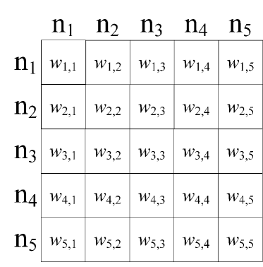
(a) Normal adjacency matrix

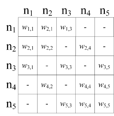
(b) Sparse adjacency matrix

Figure 7: Examples of the normal adjacency matrix and sparse adjacency matrix, where node size is 5, and the number of most related nodes is 3 in (b).

Computational complexity of existing models: Some dynamic GCN methods use the matrix manipulation of two embedding matrices $\mathbf{E_{1}}$ and $\mathbf{E_{2}}$ to obtain a dynamic adjacent matrix $\mathbf{A}$ as shown in Fig. 7(a),

$$\mathbf{A}=\mathbf{E_{1}} \mathbf{E_{2}}^{T}$$ (11)

$$\mathbf{E_{1}},\mathbf{E_{2}}\in\mathbb{R}^{N\times H},\; \mathbf{A}\in\mathbb{R}^{N\times N}$$ (12)

where $H$ is the hidden data size [9]. Some methods apply a learnable matrix, which ignore the spatial sparsity of nodes and require a quadratic computational complexity in a graph convolution process [10]. In addition, attention-based algorithms use the data-driven method to construct a weighted matrix dynamically [33], i.e.,

$$Attention(\mathbf{Q},\mathbf{K},\mathbf{V}) =\text{softmax}(\frac{\mathbf{Q}\mathbf{K}^{T}}{\sqrt{d_{k}}})\mathbf{V}.$$ (13)

$$\mathbf{Q},\mathbf{K},\mathbf{V} \in\mathbb{R}^{N\times H}$$ (14)

$\mathbf{Q}$, $\mathbf{K}$, and $\mathbf{V}$ are Queries, Keys, and Values in the attention modules, respectively. From (13), $\mathbf{Q}\mathbf{K}^{T}$ calculates the scores of each pair of nodes, producing a weight matrix like the one in Fig. 7(a). Therefore, those attention-based methods also have $\mathcal{O}(N^{2})$ computational complexity in calculating the attention values.

Computational complexity of AIMSAN : The proposed SAN layer applies the spatial sparsity of nodes into the cross-attention process, by using (6). Here, we analyse the computational complexity in calculating $\mathbf{A^{i}}$ in (4). Let $\mathbf{Q}=(w_{i,j}^{1})_{N\times T}$, $\mathbf{K}=(w_{i,j}^{2})_{N\times T}$ be the outputs of two feed-forward function in (3), and the mask matrix be $\mathbf{M}=(m_{i,j})_{N\times N}$. The mask matrix can be obtained from a distance-based adjacent matrix where only connected nodes have weights or from other context-based ones that only retain the weights from the top-$k$ most related neighbors for each node. Therefore, for each traffic node, we only need to calculate the weight values for its $k$ related nodes and obtain the sparse adjacent matrix as shown in Fig. 7(b), which exhibits $\mathcal{O}(N\times k)$ computational complexity, and $k\ll N$ in practice.

V Experiments

This section first introduces the data sets, baselines, and evaluation metrics used in this paper. Then, we compare the performance of AIMSAN on three traffic datasets with its competitive peers. Finally, we perform the parameter sensitivity analysis and ablation experiments for AIMSAN.

V-A Dataset Description

We verify the performances of AIMSAN on three real-world traffic datasets (METR-LA, PEMS04, and PEMS07) with different node sizes. We list the details of three datasets in Table II.

TABLE II: Summary statistics of datasets

Datasets	Date	#Nodes	#Time Steps	Used attribute	Target attribute	Period
METR-LA	2012/03/01-2012/05/31	207	34272	Speed, time, position, weather	Speed	5mins
PEMS04	2018/01/01-2018/02/28	307	16992	Volume, time	Volume	5mins
PEMS07	2012/05/01-2012/08/07	883	28224	Volume, time	Volume	5mins

METR-LA contains traffic speed information collected from 207 loop detectors on the highway of Los Angeles County, whose period is March 1st to June 30th, 2012 [34]. PEMS04 and PEMS07 are sampled from Performance Measurement System (PEMS) on the freeway system spanning all major metropolitan areas of California. PEMS04 uses 307 sensors in the San Francisco Bay Area, and its frequently referenced period is January 1st to February 28th, 2018. PEMS07 contains 883 sensors in the Los Angeles Area, and its frequently referenced period is May to June 2012.

In the data preparation, we enrich the weather attribute of METR-LA according to the available node location information (longitude and latitude). So, we use traffic speed, time (time of day, day of week, and holiday), position, and weather information (temperature, humidity, and weather condition) for METR-LA, and set the speed as the target attribute. Due to the lack of position information for PEMS04 and PEMS07, we cannot obtain their weather information. So, AIMSAN only uses traffic volume and time information (time of day, day of week, and holiday) to predict future traffic volume. As shown in Fig. 4, AIM can easily adjust to cases of lacking different auxiliary information. Besides, three datasets are divided into the training set (70%), validation set (10%), and test set (20%) in chronological order.

V-B Baselines and Evaluation metrics

We compare AIMSAN with the following models.

• Graph WaveNet [8]: Graph WaveNet is a convolution network architecture, which introduces a self-adaptive graph to capture the hidden spatial dependency, and uses dilated convolution to capture the temporal dependency.

• DMSTGCN [9]: It is a dynamic graph neural network model that considers the influence traffic volumes on traffic speed prediction. Therefore, It designs a dual-branch structure for learning two different factors and uses a fusion strategy to obtain the multi-faceted spatial-temporal characteristics inherent in traffic data. In METR-LA, there is only one attribute (traffic speed). Therefore, temporal information is used.

• ST-MetaNet [30]: It is a deep meta-learning-based model containing the meta graph attention network and meta RNN. The weights of the two networks are dynamically generated from the embeddings of geo-graph attributes and the traffic context learned from dynamic traffic states. While PEMS04 and PEMS07 have no positional information, only other geo-graph attributes can be used.

• TGANet [27]: It is our previous work, which combines dilated temporal convolution, multi-kernel diffusion graph convolution, and sparse self-attention module to learn the spatial-temporal dynamics of traffic data from different perspectives.

Three standard metrics in traffic forecasting are 1) Mean Absolute Error (MAE), 2) Root Mean Squared Error (RMSE), and 3) Mean Absolute Percentage Error (MAPE).

$$MAE=\frac{1}{n}\sum\limits_{i=1}^{n}|\hat{y}_{i}-y_{i}|$$ (15)

$$RMSE=\sqrt{\frac{1}{n}\sum\limits_{i=1}^{n}|\hat{y}_{i}-y_{i}|^{2}}$$ (16)

$$MAPE=\frac{100\%}{n}\sum\limits_{i=1}^{n}|\frac{\hat{y}_{i}-y_{i}}{y_{i}}|$$ (17)

where $y_{i}$ and $\hat{y}_{i}$ are the real and predicted values at the $i^{th}$ time slot, respectively. $n$ is the number of time slots. Specifically, the values of MAE, RMSE, and MAPE are used to measure the prediction errors. The smaller, the better.

Besides, we propose the Improvement score ($\Gamma$) to compare two methods:

$$\Gamma=\frac{m_{1}-m_{2}}{m_{1}}\times 100\%$$ (18)

where $m_{1}$ and $m_{2}$ are metric values (like MAE) of two methods ($M_{1}$ and $M_{2}$). The positive value of $\Gamma$ denotes that $M_{2}$ is better than $M_{1}$, otherwise not.

V-C Hyper-parameters and experimental settings

There are two important hyper-parameters in AIMSAN, the head size of the attention module ($h=3$), and the output dimension of AIM ($d_{\operatorname{AIM}}=16$). The batch size is set as 32. We apply the Adam optimizer to train AIMSAN with 100 epochs. The initial learning rate is set to 1e-3 and decays to one-tenth per twenty epochs with a minimum of 1e-6. The dilated factors of TCN are set to [2, 2, 2, 2, 2, 1]. The hidden dimension of the feed-forward network is 32, and the hidden dimension of the skip connection is 256. We set the diffusion graph convolution order as $k=2$. After experimental comparisons, we use TanH and Sigmoid functions in the Fusion gate and set the hidden size of AIM as 16 (see more details in Appendix A in our supplementary file All the experiments are conducted on a GPU server with a single PNY GeForce RTX 2080 Ti (12GB memory) GPU.

V-D Comparative experiments

TABLE III: Performance comparison of baseline models and AIMSAN. The best results are highlighted in bold, and the second-best results are underlined.

Data	Model	MAE				RMSE				MAPE(%)
		15min	30min	60min	all	15min	30min	60min	all	15min	30min	60min	all
METR-LA	GraphWaveNet (2019)	2.70	3.10	3.56	3.06	5.18	6.24	7.37	6.11	6.93	8.43	10.07	8.27
	DMSTGCN (2021)	2.84	3.24	3.68	3.18	5.52	6.51	7.48	6.34	7.50	9.06	10.72	8.86
	TGANet (2022)	2.74	3.10	3.49	3.05	5.30	6.31	7.31	6.16	7.09	8.44	9.99	8.31
	ST-MetaNet (2022)	2.69	3.10	3.58	3.06	5.15	6.27	7.52	6.14	6.94	8.64	10.82	8.56
	AIMSAN (ours)	2.73	3.08	3.47	3.04	5.23	6.20	7.19	6.06	6.99	8.41	10.02	8.28
PEMS04	Graph Wavenet (2019)	18.77	20.21	22.67	20.26	29.88	31.89	35.18	31.92	13.06	14.30	15.94	14.16
	DMSTGCN (2021)	17.88	18.71	20.49	18.77	28.76	30.07	32.53	30.09	12.28	12.93	14.36	12.96
	TGANet (2022)	18.76	19.42	20.52	19.34	29.83	31.09	32.76	30.91	12.84	13.59	14.18	13.34
	ST-MetaNet (2022)	19.06	20.36	22.46	20.31	30.13	32.05	34.98	31.95	13.10	13.98	15.48	13.98
	AIMSAN (ours)	18.66	19.32	20.30	19.24	29.81	31.10	32.54	30.88	12.82	13.20	13.87	13.16
PEMS07	Graph Wavenet (2019)	19.81	21.99	25.68	22.05	31.82	35.15	40.25	35.06	8.45	9.40	11.11	9.46
	DMSTGCN (2021)	-	-	-	-	-	-	-	-	-	-	-	-
	TGANet (2022)	20.29	21.52	23.51	21.41	32.32	34.77	38.34	34.58	8.75	9.21	10.05	9.19
	ST-MetaNet (2022)	-	-	-	-	-	-	-	-	-	-	-	-
	AIMSAN (ours)	19.79	20.99	22.82	20.90	31.98	34.54	37.99	34.33	8.36	8.86	9.74	8.85

In this subsection, we compare the proposed method with four state-of-art GCN-based peers in terms of prediction accuracy, memory usage and runtime cost. In addition, we compare AIMSAN with four classic models. Due to the poor performance of those classic models, we present the related results in Appendix B in our supplementary file.

V-D1 Prediction accuracy

Table III shows the experimental results of AIMSAN and four state-of-art GCN models on the aforementioned three traffic datasets. The target attribute of METR-LA is traffic speed, but that of PEMS04 and PEMS07 is traffic volume. Each experiment is repeated five times. The average values of MAE, RMSE, and MAPE at the 3rd, 6th, 12th steps, and all steps are recorded in Table III, respectively.

Graph Wavenet and TGANet construct multiple weighted adjacent matrices to mine rich spatial-temporal correlation of traffic data. Specifically, Graph WaveNet applies fixed adjacent matrices (predefined or learned) once the training is finished. TGANet and AIMSAN construct adaptive adjacent matrices by using attention strategies. However, AIMSAN considers the dynamic of traffic data under different cases of auxiliary factors (time, position, or weather). Therefore, it constructs AIM to embed auxiliary information of the current time window and learns dynamic adjacent matrix combining the above embedding information. As a result, AIMSAN outperforms the other two methods on the three datasets.

Both AIMSAN and DMSTGCN use auxiliary information to improve prediction accuracy. The former uses auxiliary factors like time and weather, while the latter combines secondary traffic attribute. Specifically, DMSTGCN builds two branches to learn the hidden correlations between the target and secondary traffic attributes. In METR-LA, there is only a traffic speed attribute without any secondary one. Therefore the performance of DMSTGCN is worse than other deep-learning methods, which reveals that DMSTGCN is sensitive to secondary attribute. In PEMS04 and PEMS07, traffic speed and volume are available. Therefore, in PEMS04, DMSTGCN outperforms others in most cases, revealing that different traffic parameters contain hidden correlations and can be used for target attribute prediction. It’s worth noting that AIMSAN and other deep learning methods only use one kind of traffic attribute, which fails to mine the correlation among different traffic attributes. When comparing those methods using one kind of traffic attribute on PEMS04, AIMSAN has the best performance because it learns the hidden feature of auxiliary factors of traffic data and constructs an auxiliary-information-aware adjacent matrix for dynamic GCN operations. In addition, for DMSTGCN, an out-of-memory error occurs in PEMS07 due to its dual-branch structure and the large-scale node size of PEMS07. In AIMSAN, we use a sparse strategy to make it scalable toward the different scales of traffic tasks. In conclusion, when dealing with traffic prediction tasks under different node scales and data availability, AIMSAN outperforms other baselines in most cases.

TABLE IV: Comparison of AIMSAN, TGANet and DMSTGCN on overall performance. The best results are highlighted in bold, and the second-best results are underlined.

Method	METR-LA ($N$=207)			PEMS04 ($N$=307)			PEMS07 ($N$=883)
	MAE	MAPE	RMSE	MAE	MAPE	RMSE	MAE	MAPE	RMSE
AIMSAN (ours)	3.04	6.06	8.28	19.24	30.88	13.16	20.90	34.33	8.85
DMSTGCN (2021)	3.18	6.34	8.86	18.77	30.09	12.96	-	-	-
$\Gamma$	4.40%	4.42%	6.55%	-2.50%	-2.63%	-1.54%	-	-	-
TGANet (2022)	3.05	6.16	8.31	19.34	30.91	13.34	-	-	-
$\Gamma$	0.33%	1.62%	0.36%	0.52%	0.10%	1.35%	-	-	-
ST-MetaNet (2022)	3.06	6.14	8.56	20.31	31.95	13.98	-	-	-
$\Gamma$	0.65%	1.30%	3.27%	5.27%	3.35%	5.87%	-	-	-

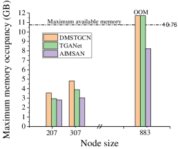
(a) Maximum GPU memory occupancy

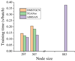
(b) Training time per batch

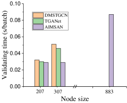
(c) Validating time per batch

Figure 8: The maximum GPU memory usage, training time and validating time of three methods

ST-MetaNet and AIMSAN are two meta-learning-based methods. The differences between them are as follows: 1) AIMSAN considers not only the positional information of the traffic graph but also the temporal information and weather conditions per sample. Therefore, it can learn more hidden temporal-spatial information. 2) Except for historical auxiliary information, AIMSAN combines future auxiliary information, like time information (holiday) and weather forecast. 3) ST-MetaNet averages the geo-graph attributes in the temporal dimension and uses averaged attributes in the following meta-knowledge learners, which may lose fine-grained information. AIMSAN uses sample-specific auxiliary information and tailors the auxiliary information by layer. In other words, the higher network layer focuses on more recent auxiliary information. The results in Table III show that AIMSAN outperforms ST-MetaNet in most cases, especially when the location information is insufficient (in the PEMS04 case). 4) ST-MetaNet stacks multiple GRU and GAN layers, and uses a meta learner in each sublayer, which results in the out-of-memory error in PEMS07 experiments.

Table IV shows the overall performance of AIMSAN, DMSTGCN, ST-MetaNet and TGANet on three datasets for 12-step prediction. In the case of single traffic data (METR-LA), AIMSAN achieves an average performance improvement of 5.12% over DMSTGCN. When DMSTGCN has enough traffic data (PEMS04) to train its dual-branch structure, the performance of AIMSAN is still similar to that of DMSTGCN, with a maximum of 2.63% performance loss. Besides, AIMSAN achieves an average performance improvement of 3.29% and 0.71% over ST-MetaNet and TGANet, respectively.

V-D2 Memory and runtime overhead

As listed in Table II, three datasets have different scales of traffic nodes. Therefore, comparing various metrics under these datasets can demonstrate the scalability of algorithms toward different scales of traffic prediction tasks. Thus, we compare the three best baselines (DMSTGCN, ST-MetaNet and TGANet) with AIMSAN. For fairness, we set the batch size to 64, as in DMSTGCN [9], to get the memory and runtime costs. For better visualization, we draw the memory usage and runtime under different node scales in Fig. 8, where the memory usage and runtime of AIMSAN grows much more slowly than its three peers. Hence, it can be applied to larger traffic prediction tasks.

V-E Parameter sensitivity and Ablation study

In this subsection, we conduct the parameter sensitivity and ablation study on METR-LA.

V-E1 Different multi-head sizes

The multi-head size of an attention module is an essential hyper-parameter in the proposed method. Therefore, we discuss the impact of head size on AIMSAN. The quantity of computation of multi-head attention increases with the head size, ranging from 1 to 8. Therefore, this work does not consider larger head sizes ($h>8$). From Fig. 9, when head size $h=3$, it has the best performance.

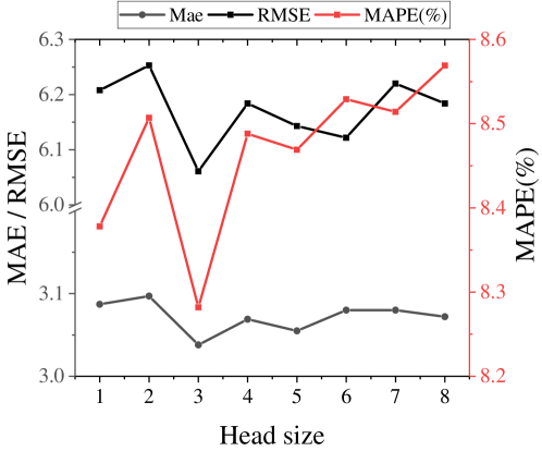
Figure 9: Performance of AIMSAN under different multi-head sizes.

V-E2 Ablation study of AIMSAN

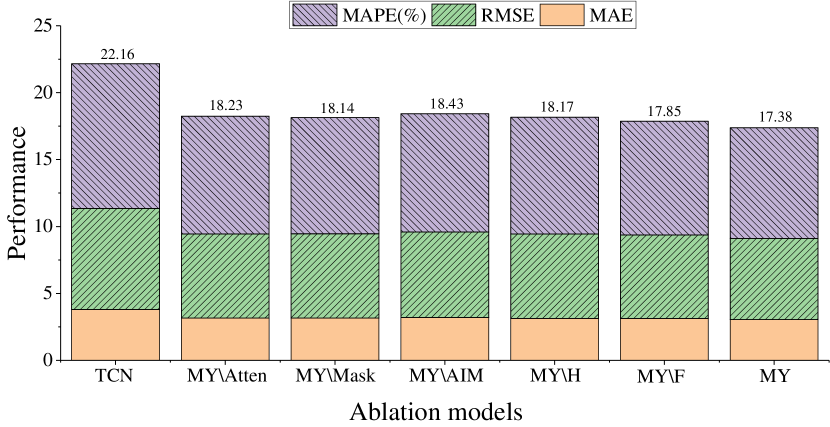
Figure 10: Ablation study of AIMSAN.

In this subsection, we study the effectiveness of each module in AIMSAN, and the results are illustrated in Fig. 10. For brevity, we use MY to represent the proposed AIMSAN. TCN denotes the simple temporal convolutional network in AIMSAN. MY\Atten abandons the SAN module in AIMSAN. MY\Mask cancels the mask operation in the SAN module. MY\AIM prunes all AIMs in AIMSAN. MY\H and MY\F cancel AIMs for historical and future auxiliary data, respectively. From the results, we can draw the following conclusions. 1) TCN can learn the temporal dependency of traffic data. However, compared with GCN-based methods, pure TCN fails to model complex spatial correlation of traffic data, which results in its worse performance. 2) The comparison between MY\Atten and MYshows the efficiency of the proposed SAN module, which can learn the dynamic spatial-temporal correlation of traffic data. 3) The results of MY\Mask and MYverify that masking operation can reduce the computational complexity, avoid interference from irrelevant nodes and further reduce the prediction error. 4) MY\AIM, MY\H, and MY\F show the positive effects of AIM.

V-E3 Ablation study on AIM

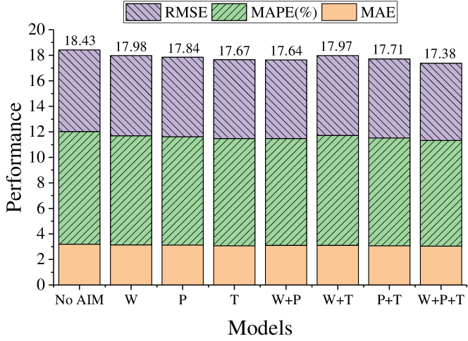
Figure 11: Ablation study for AIM.

AIM plays an essential role in AIMSAN, which contains weather (W), time (T), and position (P) information as shown in Fig. 4. Therefore, we further make an ablation study on attributes used in AIM. For brevity, we label different types of AIMSAN according to the attributes used. For example, W+P+T denotes that AIMSAN uses weather, position and time information in the AIM, and W+P denotes that AIMSAN only uses weather and position information. From the results, we can draw the following conclusion. 1) Weather, position, and temporal information can be used to mine hidden correlations within traffic data. 2) Within multiple single-attribute cases, the time attribute is superior to the other two. 3) Considering multi-attribute auxiliary factors, we obtain the best result using all three attributes.

VI Conclusion

This paper presents a deep encoder-decoder method (AIMSAN) for traffic data prediction, mainly integrating AIM and SAN modules. The former can learn the hidden feature of auxiliary information for traffic data, like weather, time and position information. In practice, we enrich the weather information of METR-LA according to the latitude and longitude of the traffic nodes. Besides, we add temporal information like holiday information to three datasets. The latter is a sparse cross-attention-based graph convolution module. AIMSAN sets the weights of a dynamic adjacent matrix according to the cross-attention values obtained by using traffic data and historical auxiliary information. Besides, the diffusion graph convolution is used in each SAN module to obtain more spatial information, whose diffusion step is 2. Extensive experiments on three public traffic datasets (PEMS04, PEMS07 and METR-LA) demonstrate that when considering multiple metrics (MAE, MSE, MAPE, memory usage and runtime), the proposed method outperforms its peers in most cases. Specifically, AIMSAN has competitive performance with the state-of-the-art algorithms but saves 35.74% of GPU memory usage, 42.25% of training time, and 45.51% of validation time on average.

Lingqiang Chen received his Ph.D. degree in control science and engineering from Jiangnan University, Wuxi, China, in 2023. He is currently a Lecturer with the School of Information & Electrical Engineering, Hebei University of Engineering, Handan, China. His research interests are anomaly detection and streaming data prediction on the Internet of Things. He has published several related papers on Inf. Sci., IEEE Trans Instrum Meas, IEEE IoTJ, Appl Soft Comput, ComCom, and Neural Comput Appl.

Qinglin Zhao received his Ph.D. degree from the Institute of Computing Technology, the Chinese Academy of Sciences, Beijing, China, in 2005. From May 2005 to August 2009, he worked as a postdoctoral researcher at the Chinese University of Hong Kong and the Hong Kong University of Science and Technology. Since September 2009, he has been with the School of Computer Science and Engineering at Macau University of Science and Technology and now he is a professor. He serves as an associate editor of IEEE Transactions on Mobile Computing and IET Communications. His research interests include blockchain and decentralization computing, machine learning and its applications, Internet of Things, wireless communications and networking, cloud/fog computing, software-defined wireless networking.

Guanghui Li received his PhD degree in Computer Science from the Institute of Computing Technology, Chinese Academy of Sciences, Beijing, China, in 2005. He is currently a professor in the School of Artificial Intelligence and Computer Science, Jiangnan University, Wuxi, China. He has published over 90 papers in journals or conferences. His research interests include Internet of Things, edge computing, fault tolerant computing, and nondestructive testing and evaluation.

Mengchu Zhou (Fellow, IEEE) received his Ph. D. degree from Rensselaer Polytechnic Institute, Troy, NY in 1990 and then joined New Jersey Institute of Technology where he is now a Distinguished Professor. His interests are in Petri nets, automation, robotics, big data, Internet of Things, cloud/edge computing, and AI. He has 1100+ publications including 14 books, 750+ journal papers (600+ in IEEE transactions), 31 patents and 32 book-chapters. He is Fellow of IFAC, AAAS, CAA and NAI.

Chenglong Dai received the MS, PhD degree in computer science and technology from Nanjing University of Aeronautics and Astronautics, Nanjing, China, in 2014, 2020, respectively. He is currently a Lecturer at the School of Artificial Intelligence and Computer Science, Jiangnan University, Wuxi, China. His research interests include Brain-Computer Interfaces (BCIs), EEG data mining, and machine learning. He has published several related papers in prestigious journals and top conferences, including IEEE TKDE, IEEE TCYB, ACM TKDD, ACM TIST, and SIAM SDM (awarded the Best Paper Award in Data Science Track). He also has served as a Recognition Reviewer for Knowledge-Based Systems, and for IJCNN 18-22.

Yiming Feng received the B.S. degree in internet of things engineering from Chongqiong University of Technology, Chongqiong, China, in 2018. He is currently a PhD candidate in the School of Artificial Intelligence and Computer Science, Jiangnan University. His current research interests include in edge computing and neural network acceleration.

References

- [1] N. Kumar and M. Raubal, “Applications of deep learning in congestion detection, prediction and alleviation: A survey,” Transportation Research Part C: Emerging Technologies, vol. 133, p. 103432, 2021.
- [2] W. Jiang and J. Luo, “Graph neural network for traffic forecasting: A survey,” Expert Systems with Applications, p. 117921, 2022.
- [3] Y. Ren, D. Zhao, D. Luo, and et al., “Global-local temporal convolutional network for traffic flow prediction,” IEEE Transactions on Intelligent Transportation Systems, vol. 23, no. 2, pp. 1578–1584, 2022.
- [4] Z. Pan, W. Zhang, Y. Liang, and et al., “Spatio-temporal meta learning for urban traffic prediction,” IEEE Transactions on Knowledge and Data Engineering, vol. 34, no. 3, pp. 1462–1476, 2022.
- [5] J. Zhang, Y. Zheng, and D. Qi, “Deep spatio-temporal residual networks for citywide crowd flows prediction,” in Thirty-first AAAI conference on artificial intelligence, 2017.
- [6] H. Yao, X. Tang, H. Wei, and et al., “Revisiting spatial-temporal similarity: A deep learning framework for traffic prediction,” in Proceedings of the AAAI conference on artificial intelligence, vol. 33, no. 01, 2019, pp. 5668–5675.
- [7] Y. Li, R. Yu, C. Shahabi, and et al., “Diffusion convolutional recurrent neural network: Data-driven traffic forecasting,” in International Conference on Learning Representations, 2018.
- [8] Z. Wu, S. Pan, G. Long, and et al., “Graph wavenet for deep spatial-temporal graph modeling,” in Proceedings of the Twenty-Eighth International Joint Conference on Artificial Intelligence, IJCAI-19, 7 2019, pp. 1907–1913.
- [9] L. Han, B. Du, L. Sun, and et al., “Dynamic and multi-faceted spatio-temporal deep learning for traffic speed forecasting,” in Proceedings of the 27th ACM SIGKDD Conference on Knowledge Discovery & Data Mining, ser. KDD ’21, 2021, p. 547–555.
- [10] M. Li and Z. Zhu, “Spatial-temporal fusion graph neural networks for traffic flow forecasting,” in Proceedings of the AAAI conference on artificial intelligence, vol. 35, no. 5, 2021, pp. 4189–4196.
- [11] F. Huang, P. Yi, J. Wang, and et al., “A dynamical spatial-temporal graph neural network for traffic demand prediction,” Information Sciences, vol. 594, pp. 286–304, 2022.
- [12] D. A. Tedjopurnomo, Z. Bao, B. Zheng, and et al., “A survey on modern deep neural network for traffic prediction: Trends, methods and challenges,” IEEE Transactions on Knowledge and Data Engineering, vol. 34, no. 4, pp. 1544–1561, 2022.
- [13] W. Huang, G. Song, H. Hong, and et al., “Deep architecture for traffic flow prediction: deep belief networks with multitask learning,” IEEE Transactions on Intelligent Transportation Systems, vol. 15, no. 5, pp. 2191–2201, 2014.
- [14] Y. Lv, Y. Duan, W. Kang, and et al., “Traffic flow prediction with big data: a deep learning approach,” IEEE Transactions on Intelligent Transportation Systems, vol. 16, no. 2, pp. 865–873, 2014.
- [15] R. Soua, A. Koesdwiady, and F. Karray, “Big-data-generated traffic flow prediction using deep learning and dempster-shafer theory,” in 2016 International joint conference on neural networks (IJCNN). IEEE, 2016, pp. 3195–3202.
- [16] X. Cheng, R. Zhang, J. Zhou, and et al., “Deeptransport: Learning spatial-temporal dependency for traffic condition forecasting,” in 2018 International Joint Conference on Neural Networks (IJCNN). IEEE, 2018, pp. 1–8.
- [17] M. Fouladgar, M. Parchami, R. Elmasri, and et al., “Scalable deep traffic flow neural networks for urban traffic congestion prediction,” in 2017 International Joint Conference on Neural Networks (IJCNN). IEEE, 2017, pp. 2251–2258.
- [18] A. A. M. Muzahid, W. Wan, F. Sohel, and et al., “CurveNet: Curvature-based multitask learning deep networks for 3d object recognition,” IEEE/CAA Journal of Automatica Sinica, vol. 8, no. 6, pp. 1177–1187, 2021.
- [19] M. Zhao, G. Xiong, M. Zhou, and et al., “PCUNet: A context-aware deep network for coarse-to-fine point cloud completion,” IEEE Sensors Journal, vol. 22, no. 15, pp. 15 098–15 110, 2022.
- [20] S. Du, T. Li, X. Gong, and et al., “Traffic flow forecasting based on hybrid deep learning framework,” in 2017 12th international conference on intelligent systems and knowledge engineering (ISKE). IEEE, 2017, pp. 1–6.
- [21] X. Hou, K. Wang, C. Zhong, and et al., “ST-Trader: A spatial-temporal deep neural network for modeling stock market movement,” IEEE/CAA Journal of Automatica Sinica, vol. 8, no. 5, pp. 1015–1024, 2021.
- [22] K. Wang, J. An, M. Zhou, and et al., “Minority-weighted graph neural network for imbalanced node classification in social networks of internet of people,” IEEE Internet of Things Journal, vol. 10, no. 1, pp. 330–340, 2023.
- [23] Z. Zhao, Z. Yang, C. Li, and et al., “Dual feature interaction-based graph convolutional network,” IEEE Transactions on Knowledge and Data Engineering, pp. 1–12, 2022.
- [24] B. Yu, H. Yin, and Z. Zhu, “Spatio-temporal graph convolutional networks: a deep learning framework for traffic forecasting,” in Proceedings of the 27th International Joint Conference on Artificial Intelligence, 2018, pp. 3634–3640.
- [25] Z. Pan, Y. Liang, W. Wang, and et al., “Urban traffic prediction from spatio-temporal data using deep meta learning,” in Proceedings of the 25th ACM SIGKDD International Conference on Knowledge Discovery & Data Mining, 2019, pp. 1720–1730.
- [26] S. Guo, Y. Lin, H. Wan, and et al., “Learning dynamics and heterogeneity of spatial-temporal graph data for traffic forecasting,” IEEE Transactions on Knowledge and Data Engineering, vol. 34, no. 11, pp. 5415–5428, 2022.
- [27] L. Chen, P. Shi, G. Li, and et al., “Traffic flow prediction using multi-view graph convolution and masked attention mechanism,” Computer Communications, vol. 194, pp. 446–457, 2022.
- [28] Y. Shin and Y. Yoon, “Incorporating dynamicity of transportation network with multi-weight traffic graph convolutional network for traffic forecasting,” IEEE Transactions on Intelligent Transportation Systems, vol. 23, no. 3, pp. 2082–2092, 2022.
- [29] K. Lee and W. Rhee, “DDP-GCN: Multi-graph convolutional network for spatiotemporal traffic forecasting,” Transportation Research Part C: Emerging Technologies, vol. 134, p. 103466, 2022.
- [30] Z. Pan, W. Zhang, Y. Liang, and et al., “Spatio-temporal meta learning for urban traffic prediction,” IEEE Transactions on Knowledge and Data Engineering, vol. 34, no. 3, pp. 1462–1476, 2022.
- [31] A. Vaswani, N. Shazeer, N. Parmar, and et al., “Attention is all you need,” Advances in neural information processing systems, vol. 30, 2017.
- [32] F. M. Shakiba and M. Zhou, “Novel analog implementation of a hyperbolic tangent neuron in artificial neural networks,” IEEE Transactions on Industrial Electronics, vol. 68, no. 11, pp. 10 856–10 867, 2020.
- [33] B. Lu, X. Gan, H. Jin, and et al., “Make more connections: Urban traffic flow forecasting with spatiotemporal adaptive gated graph convolution network,” ACM Transactions on Intelligent Systems and Technology (TIST), vol. 13, no. 2, pp. 1–25, 2022.
- [34] H. V. Jagadish, J. Gehrke, A. Labrinidis, and et al., “Big data and its technical challenges,” Communications of the ACM, vol. 57, no. 7, pp. 86–94, 2014.